Generalized analytic model for rotational and anisotropic metasolids
Abstract
An analytical approach is presented to model a metasolid accounting for anisotropic effects and rotational mode. The metasolid is made of either cylindrical or spherical hard inclusions embedded in a stiff matrix via soft claddings. It is shown that such a metasolid exhibits negative mass densities near the translational-mode resonances, and negative density of moment of inertia near the rotational resonances. As such, the effective density of moment of inertia is introduced to characterize the homogenized material with respect to its rotational mode. The results obtained by this analytical and continuum approach are compared with those from discrete mass-spring model, and the validity of the later is discussed. Based on derived analytical expressions, we study how different resonance frequencies associated with different modes vary and are placed with respect to each other, in function of the mechanical properties of the coating layer. We demonstrate that the resonances associated with additional modes taken into account, that is, axial translation for cylinders, and rotations for both cylindrical and spherical systems, can occur at lower frequencies compared to the previously studied plane-translational modes.
1 Introduction
Elastic or acoustic metamaterials are structures with subwavelength units that exhibit unusual macroscopic parameters within certain frequencies, such as negative mass density sheng2000 ; sheng2005 ; wu2008 , negative elastic bulk modulus fang2006 ; nemati2015 , simultaneous negative mass density and elastic bulk modulus chan2004 ; ding2007 ; cheng2008 ; lee2010 ; liu2011 ; sheng2013 , or negative density and shear modulus wu2011 ; sheng2011 , and negative index of refraction brunet2015 . Metamaterials with unconventional constitutive parameters have broadly extended the ability of manipulation and control of mechanical wave propagation. Wave control can arise from the formation of band gaps, that are the frequency bands where the propagation becomes forbidden. Differently from the Bragg band-gaps in phononic crystals sigalas1993 ; djafari1993 that are produced based on the collective effects of the periodically-arranged scatterers in the medium, the spectral gaps manifested in metamaterials originates in localized resonances of the material building-blocks. Thus, in metamaterilals the production of stop bands depends on the internal structure of the building units. Another mechanism emerged to achieve extreme material-parameters is based on space coiling liang2012 ; cummer2013 .
Over the last decade, research on anisotropic metamaterials has enhanced the ability to control sound and elastic wave propagation, leading to the proposal and fabrication of new devices milton2007 ; cummer2007 ; chan2008 ; zhang2009 ; christensen2010 ; zhu2011 ; yu2014 ; djafari2015 . The first acoustic metamaterial that was realized is a block of stiff material (epoxy) with uniformly (or periodically) dispersed locally resonant structural units that consist of a high-density lead sphere coated with a soft material. This material exhibits resonance-based spectral-gaps in low-frequency regime where the sonic wavelength is of two orders of magnitude larger than the lattice constants. Thus, this designed material was a major progress as sound attenuation is challenging in low frequencies. An analytical model has been proposed to capture the essence of physics dealing with this type of materials sheng2005 . Since in practice the lead sphere and the host are much stiffer compared with the coating material, in this model the host and coated sphere have been approximated to be rigid within the long-wavelength limit. Considering the two-dimensional (2D) system with coated cylindrical inclusions, and three-dimensional (3D) with coated spheres, effective dynamics of the metasolid was derived in resonance-induced band-gap regimes related to the translational motions. Analytical expressions were given for the effective mass density which becomes negative near the resonance.
In this paper, generalizing the simple model proposed in Ref. sheng2005 , we describe the dynamics of the 3D three-component composite taking into account the rotational motions of the lead cylinder or sphere, and the matrix. It is shown that when the inclusions are cylindrical, because of their geometrical anisotropy, wave propagation in the direction perpendicular to the axis of cylinders gives rise to different effective density in comparison with the effective density describing the propagation perpendicular to that axis. Components of the anisotropic effective density are given through analytical expressions. Furthermore, we introduce and analytically calculate the effective density of the moment of inertia, as a parameter that describes the effective rotational mode of the material. It has been previously demonstrated that, when the cladding is very soft, the stop-band frequency can be very low sheng2000 . This makes such a composite with a practical size interesting for various applications including sound and vibration isolations. Here, allowing for additional degrees of freedom (DOFs) related to rotational motions and translation along cylinder axis, we show that the model predicts spectral gaps characteristic for each mode of propagation. In particular, with the material components chosen in Ref. sheng2005 , we demonstrate that in the case of spherical inclusions, the band gaps related to rotational mode occur in lower frequencies compared with those corresponding to translational modes, where the respective effective parameters become negative. Also, for the case of cylindrical inclusions, comparison between the stop bands for translational modes along and perpendicular to the cylinders shows that those that occur along the cylinder axis are formed at lower frequencies. In general, for materials made of spherical or cylindrical inclusions, we analyze the occurrence of local resonances related to each mode on the frequency axis, as function of coating-material properties. It turns out that accounting for additional DOFs that results in additional propagation modes improve notably the tunability of the material in terms of size and relevant frequencies. This is significant for applications such as sound and vibration proofing, which requires small-size materials enabling the low-frequency wave attenuation.
Rotational modes in periodic solid composites have been previously studied milton2007 ; zhao2005 ; liu2011 ; peng2012 ; guenneau2013 ; huang2014 ; peng2013 . Rotary resonances have been estimated by a simple model in 2D square lattice of glass cylinders in epoxy zhao2005 . Numerical analysis was performed to obtain double negative properties, for density and bulk modulus, by utilizing simultaneously the local translational and rotational resonances of a chiral microstructure with a unit cell of three-component solid media composed of a chirally soft-coated heavy cylinder core embedded in a elastic matrix liu2011 . Periodic system of rotating resonators coated by an anisotropic heterogeneous elastic material embedded in a matrix, which was modeled by an asymptotic approach, has been reported to produce negative refraction guenneau2013 . Thus, by modelling the anisotropic material that is placed between the core and matrix as ligaments, and by coupling the translational motions with rotations, it has been numerically demonstrated that this structured medium could be employed for lensing and mode localization. Due to simultaneous translational and rotational local-resonances, a metasolid made of a chiral microstructure with a single phase material served as a system to experimentally achieve negative refraction huang2014 . Accounting for rotational modes, a mass-spring model was used to reproduce band gaps in a 2D phononic crystal made of rigid cylinders in epoxy peng2012 . This model was enhanced to describe dispersion relation for rotational modes of a 2D square array of rubber-coated steel cylinders in epoxy peng2013 . However, no analytical approach for rotational metasolids based on full elastodynamics has been reported so far.
Here, we study rotational modes and analyze their associated homogenized properties by modeling analytically the classical three-component subwavelength structures through taking general assumptions and using direct first-principle elastodynamics without any fitting parameters. This offers us not only essential physical insights for the effective dynamics of the metasolid but also a quick and efficient guide to design materials with local rotational-resonances. Additionally and in parallel, for each mode we have systematically calculated the effective parameters of the metasolid based on the discrete mass-spring modeling, and compared the results with those arising from the continuum elastodynamic model. This comparison clarifies the limits of the mass-spring based model, in particular in terms of describing the effective-material dynamics related to the second local-resonance phenomenon that manifests itself for all translational and rotational modes.
In the following, we introduce the elastodynamics equations at microscale in Sec. 2 for an arbitrary shape of the inclusions. We then study the case of cylindrical inclusions in Sec. 3, followed by the analysis for spherical inclusions in Sec. 4. In Sec. 5, the effective parameters for translational and rotational modes are calculated for the homogenized media including microscopically either cylindrical or spherical resonators. In the concluding Sec. 6, the main results of the paper are briefly summarized.
2 Microscale equations
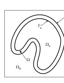
The unit cell under consideration consists of a hard inclusion embedded in a hard matrix via a soft cladding (Fig. 1). The interfaces and located between and , and between and , respectively, are assumed to be perfect. The materials constituting and are very stiff with respect to the material forming . For this reason, and within the long-wavelength limit, we make the assumption that the inclusion and matrix are rigid while the cladding is linearly elastic sheng2005 ; bonnet2015 .
The elastodynamic formulation of the unit-cell system is based on the assumptions that only the cladding is deformable and that the displacements of the inclusion and matrix are small and the strains inside the soft layer are infinitesimal. Consequently, the kinematics of the inclusion and the matrix can be formulated by
| (1) |
where , is the position vector relative to a the origin of a 3D space, and represents the displacement field generated by a translational displacement vector and an infinitesimal rotation characterized by the 3D vector . Considering the time-harmonic motion of the foregoing unit system, we write , , and , where and is the angular frequency. The motion of the cladding made of a linearly elastic isotropic homogeneous material is described by the following Navier equation together with the displacement continuity across the perfect interfaces and :
| (2a) | |||
| (2b) | |||
where and are the Lamé constants and is the mass density of the coating material.
For later use, it is convenient to introduce the Helmholtz decomposition:
| (3) |
where is a scalar field and a vector field. Using Eq. (3), the equation (2a) can be recast into the following ones
| (4a) | |||||
| (4b) | |||||
where and with and being the celerities of the longitudinal and transverse elastic waves, respectively, in an infinite linearly elastic isotropic medium. In the following, we shall analytically solve the Helmholtz equations (4) with the boundary conditions (2b) for two special cases of major interest.
3 Media with cylindrical inclusions
The first special case concerns a material with structural units consisting of three coaxial cylinders of height , uniformly or periodically distributed. The inner cylinder is a long revolution one of radius while the outer cylinder is bounded by an inner cylinder of circular cross-section of radius and an outer cylindrical surface with square cross-section (Fig. 2a).
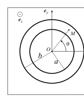
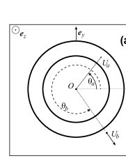
Regarding the geometry of the unit cell, it is convenient to use the cylindrical coordinates associated orthonormal vectors , , and (Fig. 2b). As it was assumed in Sec. 2, the inner and outer cylinders are rigid, whereas the cylindrical cladding is deformable. In addition, since the dimensions of the unit cell are such that , the six DOFs of the motion of relative to can be reduced to four: two translations in the transverse plane, one translation along the cylinder axis and one rotation about the latter. Thus, with no loss of generality, the boundary conditions (2b) for the cladding (Fig. 3) can be written as ()
| (5) |
where represents the amplitude of the displacement in the plane direction resulting from the rotation of by the angle around . The last term in the above expressions stands for the axial translation, with the amplitude of the displacement along . The last DOF, i.e. the rotation around the common axis , is proportional to , where is the infinitesimal amplitude of the rotation. To link the general form of the boundary conditions (2b) to Eq. (5) associated with the case of cylindrical inclusions, it is obvious that and (Fig. 3).
Considering the cylindrical nature of both the geometry and boundary conditions, the displacement field is clearly independent of the axial coordinate , thereby the potentials and are also independent of . Moreover, following Love Love44 , can be chosen to take the form . The condition in Eq. (3) is now satisfied if and only if is independent of . Thus, the potential can be expressed as .
The general form of the solutions to the Helmholtz equations (4) can be written as
| (6a) | |||
| (6b) | |||
| (6c) | |||
where (resp. ) stands for the -order Bessel function of the first (resp. second) kind. In these solutions, , , , , , , , , , and are unknown constants to be determined.
Boundary conditions (5) and Helmholtz decomposition (3) expressed in cylindrical coordinates lead to
| (7a) | |||
| (7b) | |||
| (7c) | |||
Now, we are able to determine all unknown constants involved in Eqs. (6).
Owing to the linearity of the problem, general solution for the displacement field inside the cladding can be written as , where refers to the translation in plane, to the axial displacement in direction, and to the rotation around the axis . The first displacement field can be expressed as
| (8) | |||||
where the first four terms, and the last four terms describe the displacements generated by the translations along -axis and -axis, respectively. The unknown coefficients in the above expression are the solutions to the linear systems (32) and (33) given in Appendix A. As such, we find in different terms, the solution of the plane translation given in Ref. sheng2005 corresponding to the two DOFs related to translational motions.
The displacement due to the translation along the cylinders’ axis, i.e. , is expressed as
| (9) |
Finally the displacements related to the rotational motions are provided by
| (10) |
After applying the boundary conditions (7), we obtain explicitly 111In the limit , i.e., making disappear the rigid core, the results presented in Ref. bonnet2017 can be easily obtained as a particular case of these general expressions.
| (11) | |||||
| (12) | |||||
It is important to note that, these axial and rotational contributions of the motion involves only (and not ). This is due to the state of shear dictating such kinematics. This constitutes a key point in order to achieve an anisotropic effective density, and obtain different characteristics for different directions.
We now use the equations of motion and the stresses that are known in the cladding, to deduce the relation between the displacements of the core cylinder and the embedding matrix. The equations of motion are written as
| (13a) | |||
| (13b) | |||
where is the mass of the core cylinder with the density , and is its moment of inertia. The stress tensor , with the transpose of and the identity matrix, is known since the displacement in the cladding is fully determined. After some simple calculations, we obtain the relationship between displacements of the core and the matrix, as follows
| (14) |
where . The expressions of and , involved in plane translational motion are given in the Appendix A [Eqs. (35)], which can also be found also in Ref. sheng2005 . The other components related to axial translation and rotation are expressed as
| (15a) | |||
| (15b) | |||
| Material | Epoxy (matrix) | Silicone (cladding) | Lead (core) |
|---|---|---|---|
| [] | |||
| [] | |||
| [] |
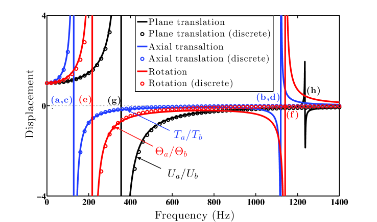
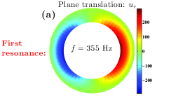
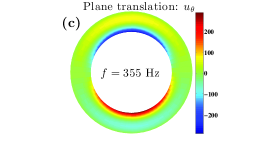
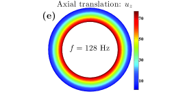
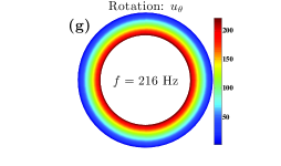
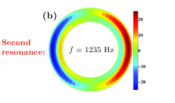
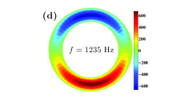
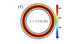
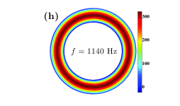
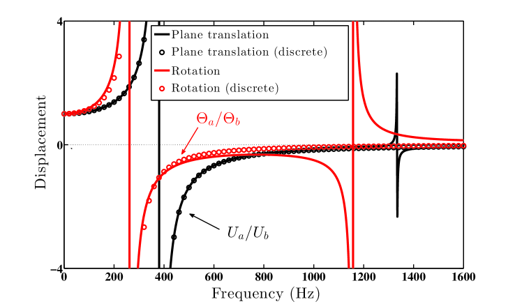
Fig. 4 shows the evolution of the displacement of the core cylinder for the three modes in function of frequency, represented by , and , using the same material properties as in Ref.sheng2000 , that are shown in Table 1 and geometrical parameters with the filling fraction for coated cylinders being 40%, 5.0 mm for the radius of the lead cylinder, and the coating thickness is 2.5 mm. For these modes of plane translation, axial translation, and rotation, the displacement field patterns inside the cladding close to the first and second resonance frequencies are depicted in Fig 5. Through Fig. 5, we observe that the field amplitudes are maximum on the boundary of the rigid cylinder at the first resonance frequency, while it is maximum inside the cladding at the second resonance frequency. The field patterns in Fig. 5a to Fig. 5h correspond to the frequency points (a) to (h) in Fig. 4. Behaviors of and are similar to that of , although obviously the resonances relating to different types of motions, when , are located at different frequencies. Indeed, the first resonances for axial, rotational and plane modes are obtained, respectively, at Hz, Hz and Hz. These resonances concern rigid-body mode insofar as the core vibrates as a whole within the elastic cladding. In this case, the dynamics of the structural unit suggests that the unit can be reasonably assimilated to a simple mass-spring system for the translational huang2009 as well as rotational mode bonnet2015 , by taking the hard cylinder as the mass, the cladding as the spring, which is attached to the mass on one side and to the rigid matrix on its other side. The mass-spring system is exited by the motion of the matrix.
Based on this mass-spring model the first resonance frequencies , , and for plane translation, axial translation, and rotation motions, respectively, can be obtained as follows
| (16) |
where . With our present configuration, the above formulas give Hz, Hz, and Hz. The good agreement with the resonance frequencies from the continuum model that is observed allows us a very fast and simple estimation of the first resonance frequencies, especially in terms of geometrical and material parameters associated with each constituent. To obtain the displacement based on the mass-spring model, we need to calculate the effective spring constants for each of the translational and rotational modes. The corresponding expressions for the effective spring constants in terms of microscale material parameters, relating to the three modes, are found in Appendix B.
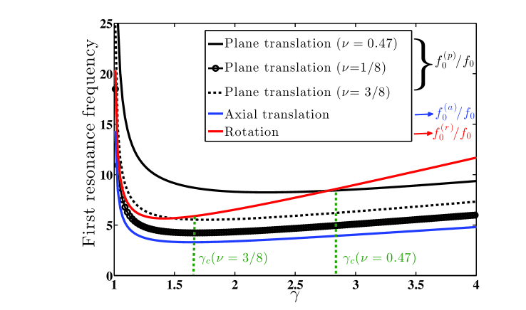
The study of relations (16) makes it possible to demonstrate that always remains smaller than the other two resonance frequencies, whatever the geometrical parameters and material properties of the coating layer. This can be observed in Fig. 6. The relations (16) also show that unlike the Poisson’s ratio , the Lamé coefficient does not change the positions of the frequencies , , and relative to each other. More precisely, for Poisson’s ratio laying in the interval , the rotational resonance always manifests itself at higher frequency compared with the plane translation resonance (), whereas for Poisson’s ratio the relative position of these two frequencies evolves with the form factor . This implies that for small inclusions such that , we have , and vice versa otherwise; where is the unique solution to the equation , i.e., . We note that is an increasing function, varying from for , to about when . Fig. 6 illustrates these remarks; in particular it shows the evolution of with for three representative values of : (), (), and that is the value for the structure studied in particular in this paper (Table 1), laying also in the interval .
Although, as seen in Fig. 4, the mass-spring model describes well the dynamics of the material at lower frequencies including the first resonances, it fails to predict the second resonance behavior for all of the three modes. This is due to the fact that the displacement field at the second resonance which is mainly produced by the standing waves inside the coating layer, while the lead cylinder follows the motion of the matrix and remains practically at rest (see Ref. sheng2005 for plane translation mode). We know that the spring, modeling the coating layer, has been assumed to be massless, and consequently this discrete model by its construction cannot describe the second resonance. That being said, if we consider a more complex discrete model by taking into account a mass for the mode-related springs a second local resonance in the elastic medium will appear. However, the outcome of latter model does not correspond to that of continuum model; particularly because in the mass-spring model the springs function in one dimension, while at the second local resonance, the displacement fields in the coating layer can be distributed in three dimensions taking, e.g. the shear effects into account. The distribution of displacement field in the plane for each of the three modes is shown in Fig. 5, close to the first and to the second resonance frequencies. In this figure, comparison of the field pattern at the first resonance for either of the modes with those arising from the same mode but at the second resonance, shows that at the second resonance the displacement field is distributed in space to a significantly greater extent than that related to the first resonance. In addition, the evaluation of the spring constants is performed in a quasi-static regime, which is further from the frequency-dependent nature of the second resonance occurring inside the elastic layer at higher frequencies. The resonance frequencies in Figs. 5a to 5h, correspond to the points (a), (b), …, and (h) in Fig. 4. The second resonance of the structure almost coincides with the first cladding resonance. This first cladding frequency can be estimated by searching for the first root of the determinant, which is a classical technique for modal analysis. In fact, we can proceed to find the solutions, by imposing a zero-displacement for the lead cylinder within the continuum model, assuming that the resonance occur only inside the elastic medium. Thus, we are led to determine the first root of , , and in order to find the second resonance frequency of the plane translation, axial translation, and rotation mode, respectively, through the following equations
| (17) | |||||
We refer to the equation (32) in Appendix A for the derivation of the first relation and the definition of the associated block matrix . The two last relations arise from the equations (11) and (12). The first and second local-resonance frequencies related to different modes, and calculated by different methods, are collected in Table 2, in order to easily compare these values associated with their respective method of calculation. In particular, it can be noticed that the relations (3) provide good estimations of the second resonance frequencies.
| Frequency | Plane (Hz) | Axial (Hz) | Rotation (Hz) |
|---|---|---|---|
| Continuum model: R1 | |||
| Discrete model : R1 | |||
| Continuum model: R2 | |||
| Estimation: R2 |
4 Media with spherical inclusions
Here, we study the same kind of problem as in the previous section with the only difference that the geometry of the structural unit is changed: the cylinder of radius and height is replaced by a hard ball of radius . An embedding matrix has now spherical cavities of radius , that are filled with the hard spheres and a concentric elastic cladding such that (Fig. 2a). All these structural components are made of the same materials as in the case of cylindrical system (see Table 1), so that the same simplifications can be applied to the corresponding kinematics. By virtue of the analysis in the previous section with coaxial cylinders, it is evident to claim, without any calculations, that for an arbitrary motion of the embedding matrix as a rigid body, the same type of motion is induced for the embedded hard ball. The superposition principle, verified for the previous case, suggests us that translations and rotations are totally uncoupled. A translation in a fixed direction or a rotation around a fixed direction, will lead, respectively, to the same translation or rotation for the hard ball, but with possibly different amplitude and/or phase.
Moreover, assuming a total isotropy of the problem, it is now convenient to consider, independently, only one translation in a certain direction and one rotation around a fixed axis to describe the whole kinematics of this problem. The former problem regarding the translational mode based on the continuum model has been solved in Ref. sheng2005 . In fact, regarding the translational mode, we only need to replace the Bessel functions in the cylindrical system by spherical Bessel functions and use the formalism explained in Appendix A. The aim of this section is to describe the kinematics of the rotational mode according to the continuum model, and compare with its counterpart built upon the discrete mass-spring model. Related equations of motion to be solved, for the cladding zone and its boundaries are stated as follows
| (18a) | |||
| (18b) | |||
Without loss of generality, we can choose (see Fig. 2b for the coordinate system), so that the solution is of the form . The equation (18b) becomes , with the boundary conditions , following (18b). We can find the solution explicitly in terms of the first order spherical Bessel functions of the first -- and second -- kind :
| (19) | |||||
As in Sec. 3, we derive the relation between the displacement of the lead sphere and the embedding matrix by applying the equation of motion for the coated sphere, and using the fact that the stresses in the cladding can be known through the displacements [Eq. (19)]:
| (20) |
where the moment of inertia of the hard sphere around . We finally obtain
| (21) |
provided that
| (22) |
Evolution of rotational displacement , and translational displacements of the lead sphere with frequency are shown in Fig. 7, for a medium with the filling fraction 47%, the lead sphere radius cm, and the thickness of the coating layer is cm. We note that, here also, with our material and geometrical parameters, the first two local resonances of the rotational mode occur in lower frequencies compared to those of translational mode, as in the case of cylindrical inclusions. The first resonance frequencies for the translation Hz and for rotational Hz. Similarly to the case of cylindrical system, the frequency of these resonances that correspond mainly to the vibration of the core sphere can be estimated through mass-spring models, leading to the following expressions
| (23) |
With our specific parameters, the above formulas give Hz and Hz, which are quite close to those obtained by the continuum model, in particular for the translation mode. Based on the mass-spring model, the displacement of the hard sphere can be obtained following the calculation of spring constants equivalent of the elastic layer [see Eqs. (37) in Appendix B]. Because of the physics of the second resonances in the cladding, we see here also from Fig. 7, that the mass-spring model ignore these resonances.
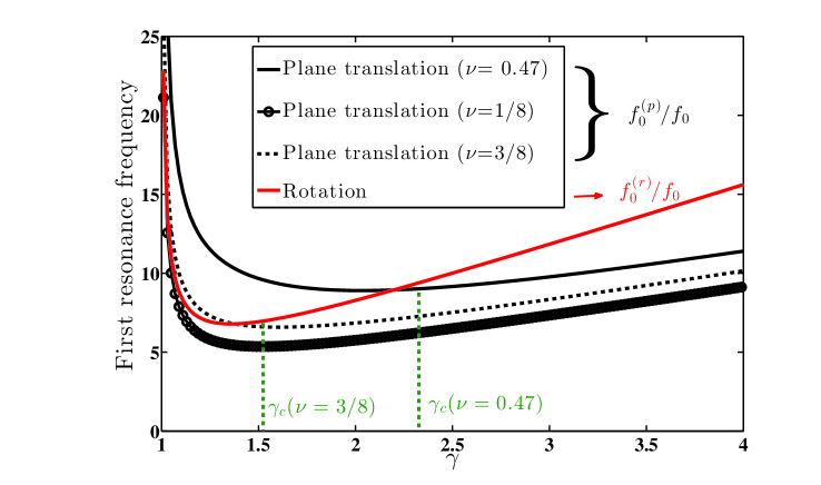
The study of the equations (23) leads to the similar conclusions as in Sec. 3. Indeed, as long as , the rotational resonance frequency is higher than the translational resonance frequency . For , the relative positions of these resonances evolves with the parameter : for the small size inclusions , we have , and vice versa otherwise (Fig. 8). The quantity is the unique solution to the equation , which is an increasing function between for , and when . Fig. 8 shows the evolution of with for three values of : (), (), and that is the value corresponding to displacement behavior in Fig. 7.
5 Effective-medium properties: Metasolids
The knowledge of the kinematics of the cladding is of great interest to go forward in the dynamical homogenization of the whole structure, with the hard coated cylinder or sphere. Indeed, our purpose is now to describe the homogenized behavior of the hard inclusion, the cladding and the matrix; and to obtain the key effective-parameters of the medium.
5.1 Homogenization for translational modes
For a given translation of the embedding matrix , we aim at finding the equivalent density for the embedded solid (sphere or cylinder) and the cladding, subject to the induced translation . The knowledge of the stress distribution in the cladding permits us to evaluate the total force applied on the cladding by the matrix, and subsequently to derive the homogenized density. Indeed we can write
| (24) |
where is the volume of the region occupied by the hard inclusion and the cladding , i.e. the region , that is bounded by the surface . The frequency-dependent effective density is defined for each point inside and must coincide with the static effective value given by , with and being the filling fraction of the coated solid and the cladding, respectively, such that .
In order to obtain the effective density for the whole unit cell, it remains to include the density of the matrix , so that we can finally set , where , and stand for the filling fraction of the coated solid, the cladding and the embedded matrix, respectively, such that .
The case of spherical inclusions has been studied in Ref. sheng2005 , through a result with an analytical expression 222Note that there is a mistake in the given expressions of , , and [Eqs. (24), (25), (32) and (33) in this paper]. The terms involved in and and involved in and should be multiplied by . However, the graphics in Fig. 2 seem to be correct.. Therefore, here we only deal with the cylindrical inclusions, where in particular an anisotropic aspect appears due to the fact that we take into account not only the plane-translation mode, but also the axial mode. Inserting in (24), the decoupling between the plane and axial translations leads to two different expressions for the effective density , depending on whether we are dealing with the axial or plane translation. The anisotropy due to the geometrical configuration of the unit cell is obviously the cause for the anisotropy of the effective mass density. We must consider the effective density as a second order tensor, and rewrite Eq. (24) as . Thus, the final expression will be
with ()
| (25) |
| (26) |
where the elements of the block matrices are defined in Appendix A. Fig. 9 shows the evolution of with frequency, where we assume that matches with the static value .
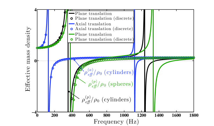
The evolutions for the axial or plane translations are qualitatively similar, but quantitatively different in that becomes negative at a lower frequency compared to in accordance with the fact that the first resonance occurs for the axial mode (Fig. 4). We explained in Sec. 3 that the (first) resonance of the axial should emerge at lower frequency, independently of the micro-structural parameters. This can be of particular interest, given that it is more challenging to make attenuate low-frequency waves. We note, however, that the resonance band where the mass density becomes negative, may also be less wide for the axial mode. With the present material and geometrical parameters, the band width for the axial mode Hz, while that of plane-translational mode Hz.
The effective masses related to the plane translations for media with cylindrical or spherical inclusions, and axial translation modes, can also be calculated through the discrete mass-spring model. Once the effective spring constants (plane translation) and (axial translation) are obtained (Appendix B), and the displacements (plane translation), (axial translation) calculated (Secs. 3 and 4), the equations of motion for the respective mass-spring systems lead easily to the frequency-dependent effective-masses for plane and axial translations. Fig. 9 shows these effective masses divided by the volume of the structural unit, in function of frequency. We see that the discrete model predicts well the dynamic effective densities in low frequencies including the first negative region for both plane and axial translation modes. Expectedly, from the analysis on the resonance behaviors in Secs. 3 and 4, the second negative regions of effective mass densities that correspond to the second resonances (Figs. 4 and 7), are ignored by the discrete model for both modes and medium micro-geometries (Fig. 9).
5.2 Homogenization for rotational modes
In order to obtain the effective parameter related to the rotations, we apply first the angular equation of motion to the sub-structure formed by the hard inclusion and the cladding. It reads
| (28) |
where denotes the resulting moment of inertia around for the embedded rigid body and its surrounded cladding that move in phase. Following a similar procedure regarding translation modes, we can establish the expression of the density of the moment of inertia such that . Since this unusual quantity is obviously intensive in thermodynamic sense, its homogenization in the medium should be possible. Tensorial behavior is involved to ensure the anisotropic aspects of the problem, hence we write : .
Similar to the case of translations, the formal expression of the effective density of the moment of inertia can be written as .
The spherical system gives rise to an effective density of moment of inertia , with
| (29) |
provided that
| (30) |
where,
The isotropy of is clear and it is evident that coincides with the static value in the quasistatic limit ; with , , and .
Employing the same method that was used in the case of spherical system, for media with cylindrical inclusions, we obtain
| (31) |
with
where , , and .
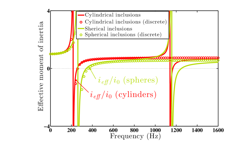
Fig. 10 presents the behavior of in function of frequency, for media with cylindrical and spherical inclusions. This behavior with the negative values near rotational stop-band frequencies is similar to that we observed earlier for the effective mass densities. Here also, after calculating the spring constants for analogous mass-spring system (Appendix B), and then obtaining the displacement (Figs. 4 and 7), the effective mass densities can be expressed according to the discrete model. Again, from Fig. 10 we observe that negative mass densities related to the lower resonance frequency band are appropriately described by the discrete model, while those associated with the higher frequency band, that is largely due to the rotational resonance inside the coating, are disregarded.
6 Summary and conclusions
A metasolid composed of a distribution of either cylindrical or spherical hard inclusions coated by a soft material has been studied. Generalizing an existing continuum model sheng2005 that describes resonance-induced band gaps related to plain-translational modes, we provide analytical analysis to investigate anisotropic properties in the case of cylindrical inclusions, and also rotational modes for both cylindrical and spherical systems.
We showed that the translational mode along the cylinders’ axis and the rotational mode in both cylindrical and spherical systems could generate band gaps at low frequencies. The band gaps that originate in local resonance phenomena at long-wavelength regime, are tunable in terms of frequency by changing the coating’s elastic properties and geometrical parameters of the structural unit. Furthermore, for all translational and rotational modes we found that the discrete mass-spring model could provide appropriate description of the material’s kinematics including first resonances, but neglects the second resonances that occur at higher frequencies and mainly arise from resonances inside the coating. The mass-spring model also provides simple analytical expressions allowing us to study easily the kinematics of first resonances in terms of the material parameters. We demonstrated that, while the macroscopic material dynamics is dictated by the effective mass densities for translational modes, it is characterized by its effective moment of inertia regarding the rotational modes. Through analytical expressions, it was shown that components of frequency-dependent anisotropic effective densities for translational modes, and effective density of moment of inertia for rotational mode, become negative near corresponding resonance frequencies. These effective parameters have been also calculated based on the mass-spring model, and their limits have been clarified by comparison to the continuum model.
These results establish a step forward for metasolid characterization via introducing the density of moment of inertia as an effective-medium parameter. They give insight to improving the tunability of the metasolid for various applications, such as sound and vibration isolation, and can serve as a physical-based quick guide for optimal design of the material to exhibit desired properties.
Acknowledgements
The authors acknowledge support from the French National Research Agency (grant no. ANR-13-RMNP-0003-01 and ANR-11-LABX-022-01).
Appendix A Expressions of the solutions to Helmholtz equations
Here, we will give the explicit form of the solutions to the Helmholtz equations (4), combined with the boundary conditions for the case of cylindrical inclusions in Section 3. The boundary conditions (7) and the solutions (6) lead to the following first conclusions
The expressions of the unknowns and are established in the article. The coefficients , , and involved in (8) are solutions to the following linear system
| (32) |
where the matrices used in the bloc-matrix formalism are
Similarly, the coefficients , , and in (8) are determined by solving the linear system:
| (33) |
with the same notations for the matrices and , whereas . The solutions of the above linear systems can be obtained with bloc-matrix formalism, which leads to the final expression for the displacement field involved in (8).
It is easy now to compute the ratio between the relative plane translations and . Using (13), after some formal calculations, we obtain
| (34) |
with
| (35) |
where , , and .
We note that the relation (34) is not only obtained for the plane translation in direction (given after solving (32)), that is , but also for the plane translation in direction (given after solving (33)), i.e., . Although this seems clear in the physical sense, the mathematical treatment is relatively tedious.
Appendix B Expressions for effective stiffnesses according to mass-spring model
The effective stiffnesses based on the discrete mass-spring model are obtained by using the static regime of general equations (2a) for the cladding with , and by imposing zero displacement on the inner boundary of the cladding , with and , regarding Eq. (2b). The resulting force gives the spring constants for translations (plane and axial), and the resulting torque leads to the spring constant for rotational motion. The corresponding equations are
for translational and rotational motions, respectively. In the above equations is the spring constant, equivalent of the coating-layer that is represented by a spring in 1D tension/compression, and related to the (plane and axial) translational motion of the layer. Likewise, is the spring constant describing the torsional stiffness of the coating layer that is taken to be analogous to a spring in 1D tension/compression, related to the rotational motion of the layer. For cylindrical inclusions, the expressions of these constants are obtained as
| (36) |
where , , and refer to plane translation, axial translation, and rotation, respectively. For the spherical inclusions, we obtain
| (37) |
The expressions for spring constants and for media with cylindrical and spherical inclusions can also be found in Ref. bonnet2015 .
References
- (1) Liu Z, Zhang X, Mao Y, Zhu Y Y, Yang Z, Chan C T and Sheng P 2000 Locally resonant sonic Materials Science 289 1734
- (2) Liu Z, Chan C T and Sheng P 2005 Analytic model of photonic crystals with local resonances Phys. Rev. B 71 014103
- (3) Yang Z, Mei J, Yang M, Chan N H and Sheng P 2008 Membrane-type acoustic metamaterial with negative dynamic mass Phys. Rev. Lett. 101 204301
- (4) Fang N, Xi D, Xu J, Ambati M, Srituravanich W, Sun C and Zhang X 2006 Ultrasonic metamaterials with negative modulus Nat. Mater. 5 452
- (5) Nemati N, Kumar A, Lafarge D and Fang N X 2015 Nonlocal description of sound propagation through an array of Helmholtz resonators C. R. Mecanique 343 656
- (6) Li J and Chan C T 2004 Double-negative acoustic metamaterial Phys. Rev. E 70 055602(R)
- (7) Ding Y, Liu Z, Qiu C and Shi J 2007 Metamaterial with simultaneously negative bulk modulus and mass density, Phys. Rev. Lett. 99 093904
- (8) Cheng Y, Xu J Y and Liu X J 2008 One-dimensional structured ultrasonic metamaterials with simultaneously negative dynamic density and modulus Phys. Rev. B 77 045134
- (9) Lee S H, Park C M, Seo Y M, Wang Z G and C. K. Kim 2010 Composite acoustic medium with simultaneously negative density and modulus Phys. Rev. Lett. 104 054301
- (10) Liu X N, Hu G K, Huang G L and Sun C T 2011 An elastic metamaterial with simultaneously negative mass density and bulk modulus Appl. Phys. Lett. 98 251907
- (11) Yang M, Ma G, Yang Z and Sheng P 2013 Coupled membranes with doubly negative mass density and bulk modulus Phys. Rev. Lett. 110 134301
- (12) Wu Y, Lai Y and Zhang Z Q 2011 Elastic metamaterials with simultaneously negative effective shear modulus and mass density Phys. Rev. Lett. 107 105506
- (13) Lai Y, Wu Y, Sheng P and Zhang Z Q 2011 Hybrid elastic solids Nat. Mater. 10 620
- (14) Brunet T, Merlin A, Mascaro B, Zimny K, Leng J, Poncelet O, Aristégui C and Mondain-Monval O 2015 Soft 3D acoustic metamaterial with negative index Nat. Mater. 14 384
- (15) Sigalas M and Economou E 1993 Band structure of elastic waves in two-dimensional systems Solid State Commun. 86 141
- (16) Kushwaha M S, Halevi P, Dobrzynski L, Djafari-Rouhani B 1993 Acoustic band structure of periodic elastic composites Phys. Rev. Lett. 71 2022
- (17) Liang Z and Li J 2012 Extreme acoustic metamaterial by coiling up space Phys. Rev. Lett. 108 114301
- (18) Xie Y, Popa B I, Zigoneanu L and Cummer S A 2013 Measurement of a broadband negative index with space-coiling acoustic metamaterials Phys. Rev. Lett. 110 175501
- (19) Milton G W and Willis J R 2007 On modifications of Newton’s second law and linear continuum elastodynamics Proc. R. Soc. A 463 855
- (20) Cummer S A and Schurig D 2007 One path to acoustic cloaking New J. Phys. 9 45
- (21) Ao X and Chan C T 2008 Far-field image magnification for acoustic waves using anisotropic acoustic metamaterials Phys. Rev. E 77 025601(R)
- (22) Li J, Fok L, Yin X, Bartal G and Zhang X 2009 Experimental demonstration of an acoustic magnifying hyperlens Nat. Mater. 8 931
- (23) Zhu J, Christensen J, Jung J, Martin-Moreno L, Yin X, Fok L, Zhang X and Garcia-Vidal F G 2010 A holey-structured metamaterial for acoustic deep-subwavelength imaging Nat. Phys. 7 52
- (24) Zhu X, Liang B, Kan W, Zou X and Cheng J 2011 Acoustic cloaking by a superlens with single-negative materials Phys. Rev. Lett. 106 014301
- (25) Chen Y, Liu H, Reilly M, Bae H and Yu M 2014 Enhanced acoustic sensing through wave compression and pressure amplification in anisotropic metamaterials Nat. Comm. 5 5247
- (26) Torrent D, Pennec Y and Djafari-Rouhani B 2015 Resonant and nonlocal properties of phononic metasolids Phys. Rev. B 92 174110
- (27) Zhao H, Liu Y, Wang G, Wen J, Yu D, Han X and Wen X 2005 Resonance modes and gap formation in a two-dimensional solid phononic crystal Phys. Rev. B 72 012301
- (28) Peng P, Mei J and Wu Y 2012 Lumped model for rotational modes in phononic crystals Phys. Rev. B 86 134304
- (29) Bigoni D, Guenneau S, Movchan A B and Brun M 2013 Elastic metamaterials with inertial locally resonant structures: Application to lensing and localization Phys. Rev. B 87 174303
- (30) Zhu R, Liu X N, Hu G K, Sun C T and Huang G L 2014 Negative refraction of elastic waves at the deep-subwavelength scale in a single-phase metamaterial Nat. Commun. 5 5510
- (31) Peng P, Asiri S, Zhang X, Li Y and Wu Y 2013 A lumped model for rotational modes in periodic solid composites EPL 104 26001
- (32) Bonnet G and Monchiet V 2015 Low frequency locally resonant metamaterials containing composite inclusions J. Acoust. Soc. Am. 137 3263
- (33) Love A E H 1944 A Treatise on the Mathematical Theory of Elasticity (New York: Dover)
- (34) Bonnet G and Monchiet V 2017 Dynamic mass density of resonant metamaterials with homogeneous inclusions J. Acoust. Soc. Am. 142 890
- (35) Huang H H and Sun C T Wave attenuation mechanism in an acoustic metamaterial with negative effective mass density 2009 New J. Phy. 11 013003