DESY-17-212 \prepdate d March 2024
Further studies of isolated photon production with a jet in deep inelastic scattering at HERA
Abstract
Isolated photons with high transverse energy have been studied in deep inelastic scattering with the ZEUS detector at HERA, using an integrated luminosity of in the range of exchanged-photon virtuality . Outgoing isolated photons with transverse energy GeV and pseudorapidity were measured with accompanying jets having transverse energy and pseudorapidity GeV and , respectively. Differential cross sections are presented for the following variables: the fraction of the incoming photon energy and momentum that is transferred to the outgoing photon and the leading jet; the fraction of the incoming proton energy transferred to the photon and leading jet; the differences in azimuthal angle and pseudorapidity between the outgoing photon and the leading jet and between the outgoing photon and the scattered electron. Comparisons are made with theoretical predictions: a leading-logarithm Monte Carlo simulation, a next-to-leading-order QCD prediction, and a prediction using the -factorisation approach.
The ZEUS Collaboration
H. Abramowicz24,p, I. Abt19, L. Adamczyk7, M. Adamus30, R. Aggarwal3,b, S. Antonelli1, V. Aushev16, Y. Aushev16, O. Behnke9, U. Behrens9, A. Bertolin21, I. Bloch10, I. Brock2, N.H. Brook28,q, R. Brugnera22, A. Bruni1, P.J. Bussey11, A. Caldwell19, M. Capua4, C.D. Catterall32, J. Chwastowski6, J. Ciborowski29,s, R. Ciesielski9,e, A.M. Cooper-Sarkar20, M. Corradi1,a, R.K. Dementiev18, R.C.E. Devenish20, S. Dusini21, B. Foster12,j, G. Gach7, E. Gallo12,k, A. Garfagnini22, A. Geiser9, A. Gizhko9, L.K. Gladilin18, Yu.A. Golubkov18, G. Grzelak29, M. Guzik7, C. Gwenlan20, O. Hlushchenko16,n, D. Hochman31, R. Hori13, Z.A. Ibrahim5, Y. Iga23, M. Ishitsuka25, N.Z. Jomhari5, I. Kadenko16, S. Kananov24, U. Karshon31, P. Kaur3,c, D. Kisielewska7, R. Klanner12, U. Klein9,f, I.A. Korzhavina18, A. Kotański8, N. Kovalchuk12, H. Kowalski9, B. Krupa6, O. Kuprash9,g, M. Kuze25, B.B. Levchenko18, A. Levy24, M. Lisovyi9,h, E. Lobodzinska9, B. Löhr9, E. Lohrmann12, A. Longhin21, O.Yu. Lukina18, J. Malka9, A. Mastroberardino4, F. Mohamad Idris5,d, N. Mohammad Nasir5, V. Myronenko9,i, K. Nagano13, Yu. Onishchuk16, E. Paul2, W. Perlański29,t, N.S. Pokrovskiy14, A. Polini1, M. Przybycień7, M. Ruspa27, D.H. Saxon11, M. Schioppa4, U. Schneekloth9, T. Schörner-Sadenius9, L.M. Shcheglova18,o, O. Shkola16, Yu. Shyrma15, I.O. Skillicorn11, W. Słomiński8, A. Solano26, L. Stanco21, N. Stefaniuk9, A. Stern24, P. Stopa6, J. Sztuk-Dambietz12,l, E. Tassi4, K. Tokushuku13, J. Tomaszewska29,u, T. Tsurugai17, M. Turcato12,l, O. Turkot9,i, T. Tymieniecka30, A. Verbytskyi19, W.A.T. Wan Abdullah5, K. Wichmann9,i, M. Wing28,r, S. Yamada13, Y. Yamazaki13,m, A.F. Żarnecki29, L. Zawiejski6, O. Zenaiev9, B.O. Zhautykov14
1 INFN Bologna, Bologna, Italy A
2 Physikalisches Institut der Universität Bonn, Bonn, Germany B
3 Panjab University, Department of Physics, Chandigarh, India
4 Calabria University, Physics Department and INFN, Cosenza, Italy A
5 National Centre for Particle Physics, Universiti Malaya, 50603 Kuala Lumpur, Malaysia C
6
The Henryk Niewodniczanski Institute of Nuclear Physics, Polish Academy of
Sciences, Krakow, Poland
7 AGH University of Science and Technology, Faculty of Physics and Applied Computer Science, Krakow, Poland
8 Department of Physics, Jagellonian University, Krakow, Poland
9 Deutsches Elektronen-Synchrotron DESY, Hamburg, Germany
10 Deutsches Elektronen-Synchrotron DESY, Zeuthen, Germany
11 School of Physics and Astronomy, University of Glasgow, Glasgow, United Kingdom D
12 Hamburg University, Institute of Experimental Physics, Hamburg, Germany E
13 Institute of Particle and Nuclear Studies, KEK, Tsukuba, Japan F
14 Institute of Physics and Technology of Ministry of Education and Science of Kazakhstan, Almaty, Kazakhstan
15 Institute for Nuclear Research, National Academy of Sciences, Kyiv, Ukraine
16 Department of Nuclear Physics, National Taras Shevchenko University of Kyiv, Kyiv, Ukraine
17 Meiji Gakuin University, Faculty of General Education, Yokohama, Japan F
18 Lomonosov Moscow State University, Skobeltsyn Institute of Nuclear Physics, Moscow, Russia G
19 Max-Planck-Institut für Physik, München, Germany
20 Department of Physics, University of Oxford, Oxford, United Kingdom D
21 INFN Padova, Padova, Italy A
22 Dipartimento di Fisica e Astronomia dell’ Università and INFN, Padova, Italy A
23 Polytechnic University, Tokyo, Japan F
24
Raymond and Beverly Sackler Faculty of Exact Sciences, School of Physics,
Tel Aviv University, Tel Aviv, Israel H
25 Department of Physics, Tokyo Institute of Technology, Tokyo, Japan F
26 Università di Torino and INFN, Torino, Italy A
27 Università del Piemonte Orientale, Novara, and INFN, Torino, Italy A
28 Physics and Astronomy Department, University College London, London, United Kingdom D
29 Faculty of Physics, University of Warsaw, Warsaw, Poland
30 National Centre for Nuclear Research, Warsaw, Poland
31 Department of Particle Physics and Astrophysics, Weizmann Institute, Rehovot, Israel
32 Department of Physics, York University, Ontario, Canada M3J 1P3 I
A supported by the Italian National Institute for Nuclear Physics (INFN)
B supported by the German Federal Ministry for Education and Research (BMBF), under contract No. 05 H09PDF
C supported by HIR grant UM.C/625/1/HIR/149 and UMRG grants RU006-2013, RP012A-13AFR and RP012B-13AFR from Universiti Malaya, and ERGS grant ER004-2012A from the Ministry of Education, Malaysia
D supported by the Science and Technology Facilities Council, UK
E supported by the German Federal Ministry for Education and Research (BMBF), under contract No. 05h09GUF, and the SFB 676 of the Deutsche Forschungsgemeinschaft (DFG)
F supported by the Japanese Ministry of Education, Culture, Sports, Science and Technology (MEXT) and its grants for Scientific Research
G partially supported by RF Presidential grant NSh-7989.2016.2
H supported by the Israel Science Foundation
I supported by the Natural Sciences and Engineering Research Council of Canada (NSERC)
a now at INFN Roma, Italy
b now at DST-Inspire Faculty, Pune University, India
c now at Sant Longowal Institute of Engineering and Technology, Longowal, Punjab, India
d also at Agensi Nuklear Malaysia, 43000 Kajang, Bangi, Malaysia
e now at Rockefeller University, New York, NY 10065, USA
f now at University of Liverpool, United Kingdom
g now at Tel Aviv University, Israel
h now at Physikalisches Institut, Universität Heidelberg, Germany
i supported by the Alexander von Humboldt Foundation
j Alexander von Humboldt Professor; also at DESY and University of Oxford
k also at DESY
l now at European X-ray Free-Electron Laser facility GmbH, Hamburg, Germany
m now at Kobe University, Japan
n now at RWTH Aachen, Germany
o also at University of Bristol, United Kingdom
p also at Max Planck Institute for Physics, Munich, Germany, External Scientific Member
q now at University of Bath, United Kingdom
r also supported by DESY and the Alexander von Humboldt Foundation
s also at Łódź University, Poland
t member of Łódź University, Poland
u now at Polish Air Force Academy in Deblin
1 Introduction
The isolated high-energy photons that are emitted in high-energy collisions involving hadrons are predominantly unaffected by parton hadronisation. Their production probes the underlying partonic process and can provide information on the structure of the proton. Processes of this type have been studied in a number of fixed-target and hadron-collider experiments [1, *zfp:c38:371, *pr:d48:5, *prl:73:2662, *prl:95:022003, *prl:84:2786, *plb:639:151, *atlas1, *atlas2, *cms1]. The production of isolated photons in photoproduction, where the incoming photon is quasi-real, was previously studied at HERA by the ZEUS and H1 collaborations [11, *pl:b472:175, *pl:b511:19, 14, 15]. Deep inelastic neutral current (NC) scattering (DIS), in which the exchanged photon has virtuality , has also been measured in a variety of ranges [16, 17, 18]. The analysis presented here extends an earlier ZEUS measurement of isolated photons and jets in DIS [19].
Figure 1 shows leading-order diagrams for high-energy photon production in DIS. Such “prompt” photons are emitted either by the incoming or outgoing quark or by the incoming or outgoing lepton. In the first case, the photons are classified as “QQ” photons, and the hadronic process has two hard scales: the virtuality of the incident exchanged photon and the square of the transverse momentum of the prompt photon. In the second case, the photons are denoted as “LL” and are emitted from the incoming or outgoing lepton. The present analysis requires the observation of a scattered electron, a high-energy outgoing photon and a hadronic jet. Processes in which the final state consists solely of a hard outgoing electron and a hard outgoing photon are thereby excluded. By requiring the outgoing photon to be isolated, a further class of processes in which the photon is produced within a jet is suppressed.
In the previous ZEUS publication on this topic [19], kinematic distributions of the outgoing photon and the jet were studied. Using the same data set, the analysis is extended here by measuring variables that involve two of the outgoing photon, the jet and the scattered electron. Results from a leading-logarithm parton-shower Monte Carlo [20] are compared to the measurements. Comparison is also made with two theoretical models: one at next-to-leading order (NLO) in QCD [21, 22], and one based on a -factorisation approach [23].
2 Experimental set-up
The data sample used for the measurement corresponds to an integrated luminosity of and was taken with the ZEUS detector in the years 2004–2007. During this period, HERA ran with an electron/positron beam energy of 27.5 \GeV and a proton beam energy of 920 \GeV; of data and of data111Hereafter, “electron” refers to both electrons and positrons unless otherwise stated. were used in the present analysis.
A detailed description of the ZEUS detector can be found elsewhere [24]. Charged particles were recorded in the central tracking detector (CTD) [25, *npps:b32:181, *nim:a338:254] and a silicon microvertex detector [28] which operated in a magnetic field of T provided by a thin superconducting solenoid. The high-resolution uranium–scintillator calorimeter (CAL) [29, *nim:a309:101, *nim:a321:356, *nim:a336:23] consisted of three parts: the forward (FCAL), the barrel (BCAL) and the rear (RCAL) calorimeters. The BCAL covered the pseudorapidity range to as seen from the nominal interaction point222The ZEUS coordinate system is a right-handed Cartesian system, with the axis pointing in the nominal proton beam direction, referred to as the “forward direction”, and the axis pointing towards the centre of HERA. The coordinate origin is at the centre of the central tracking detector. The pseudorapidity is defined as , where the polar angle, , is measured with respect to the axis. The azimuthal angle, , is measured with respect to the axis.. The FCAL and RCAL extended the range to to . The smallest subdivision of the CAL is called a cell. The barrel electromagnetic calorimeter (BEMC) cells had a pointing geometry aimed at the nominal interaction point, with a cross section approximately , with the finer granularity in the -direction. This fine granularity allows the use of shower-shape distributions to distinguish isolated photons from the products of neutral meson decays such as .
3 Event selection and reconstruction
The ZEUS experiment operated a three-level trigger system [24, 37, 38]. At the first level, events were selected if they had an energy deposit in the CAL consistent with an isolated electron. At the second level, a requirement on the energy and longitudinal momentum of the event was used to select NC DIS events. At the third level, the full event was reconstructed and tighter requirements for a DIS electron were made. Offline selections, similar to those of the earlier ZEUS analysis [19], were then applied.
Outgoing electrons were selected with polar angle in order to provide a good measurement in the RCAL, kinematically separated from the selected outgoing photons. Their impact point (,) on the surface of the RCAL was required to lie outside a rectangular region cm in and cm in , to give a well understood acceptance. The outgoing electrons were identified using a neural network [39], and the energy of the outgoing electron, , corrected for apparatus effects, was required to be larger than 10 GeV. The kinematic variable was reconstructed as where () is the four-momentum of the incoming (outgoing) electron. The kinematic region GeV2 was selected.
A requirement that the event vertex position, , should be within the range reduces the background from non- collisions. A further requirement for a well-contained DIS event, , was imposed where ; is the energy of the -th CAL cell, is its polar angle and the sum runs over all cells [40].
Photon candidates were identified as energy-flow objects (EFOs)333Energy-flow objects [41, *epj:c6:43, *briskin:phd:1998] were constructed from calorimeter-cell clusters and tracks, associated when possible. without an associated track, for which at least of the reconstructed energy was deposited in the BEMC. The calibration of the energies of the photon and scattered electron was taken from an earlier ZEUS analysis and used deeply virtual Compton scattering events [44]. The reconstructed transverse energy of the photon candidate, , was required to lie within the range444The upper limit was selected to retain distinguishable shower shapes between the hadronic background and the photon signal. and the pseudorapidity, , had to satisfy .
Jets were reconstructed with the clustering algorithm [45] in the scheme in the longitudinally invariant inclusive mode [46] with the parameter set to 1.0. Since all EFOs of the event were used except for the electron signal, one of the jets found by this procedure corresponds to or includes the photon candidate. At least one accompanying jet was required with transverse energy and pseudorapidity, , in the range ; if more than one jet was found, that with the highest was used.
Photons radiated from final-state electrons were suppressed by requiring that , where is the distance to the nearest reconstructed track with momentum greater than in the plane. Isolation from hadronic activity was imposed by requiring that the photon candidate possessed at least of the total energy of the jet-like object of which it formed a part. This also reduced the background of photon candidates arising from neutral meson decay.
Approximately 6000 events were selected at this stage; this sample was dominated by background events in which one or more neutral mesons such as and , decaying to photons, produced a photon candidate in the BEMC.
4 Variables studied
In the previous ZEUS publication [19], distributions of photon and jet variables were studied. In the present analysis, variables that depend on two of the three measured outgoing physical objects were studied, namely the high- photon, the leading jet and the scattered electron. They were defined as follows:
-
•
is a measure of the fraction of the exchanged-photon energy and longitudinal momentum that is given to the outgoing photon and the jet:
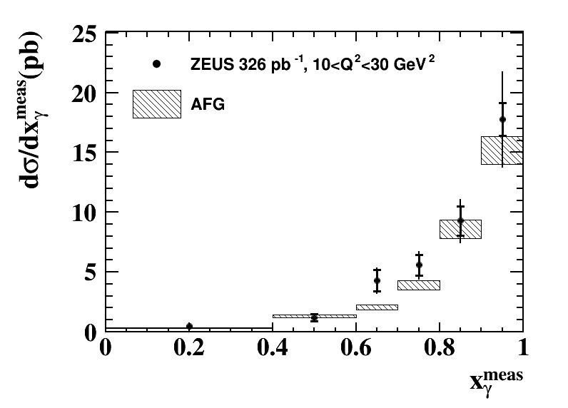
where and denote the energies of the outgoing photon and the jet, respectively, and denote the corresponding longitudinal momenta, GeV, and the Jacquet–Blondel variable is given by , summing over all energy-flow objects in the event except the scattered electron, each object being treated as equivalent to a massless particle. This variable is sensitive to higher-order processes that generate additional particles in the event;
-
•
estimates the fraction of the proton energy transferred to the outgoing photon and jet:
where GeV. This variable is sensitive to the partonic structure of the proton;
-
•
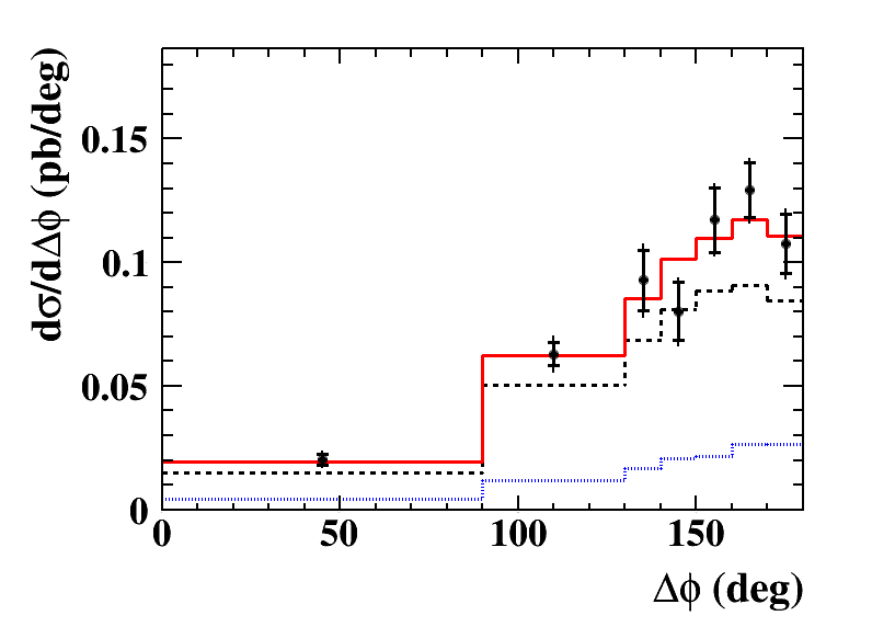
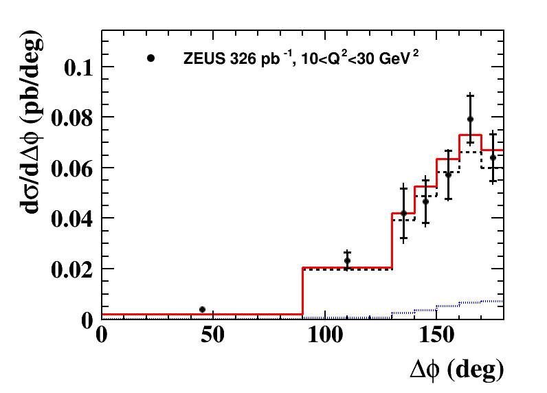
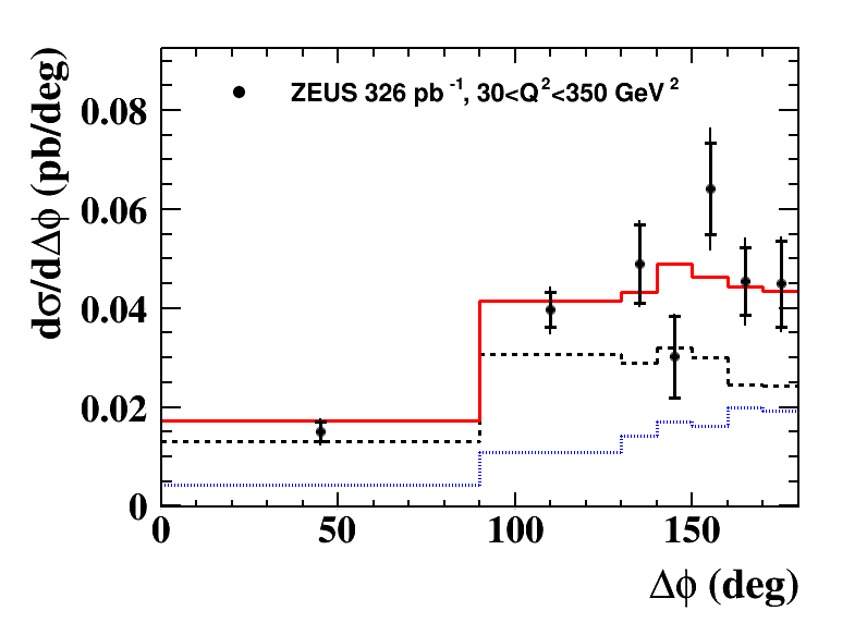
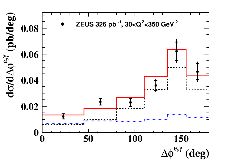
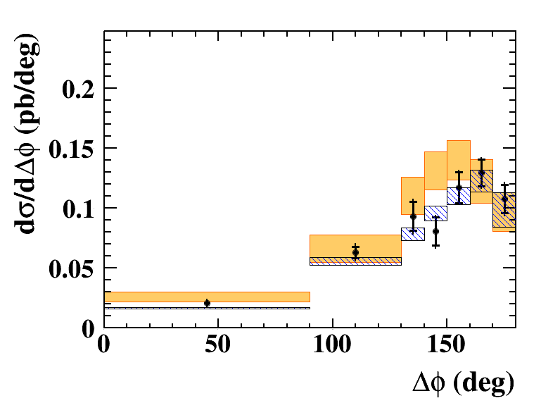
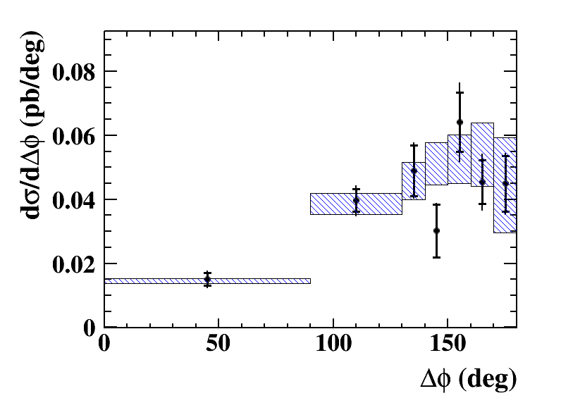
is the azimuthal angle between the jet and the outgoing photon: , where and denote the azimuthal angles of the jet and photon, respectively. This variable is sensitive to the presence of higher-order gluon radiation from the outgoing quark, which generates a contribution to the non-collinearity between the photon and the leading jet;
-
•
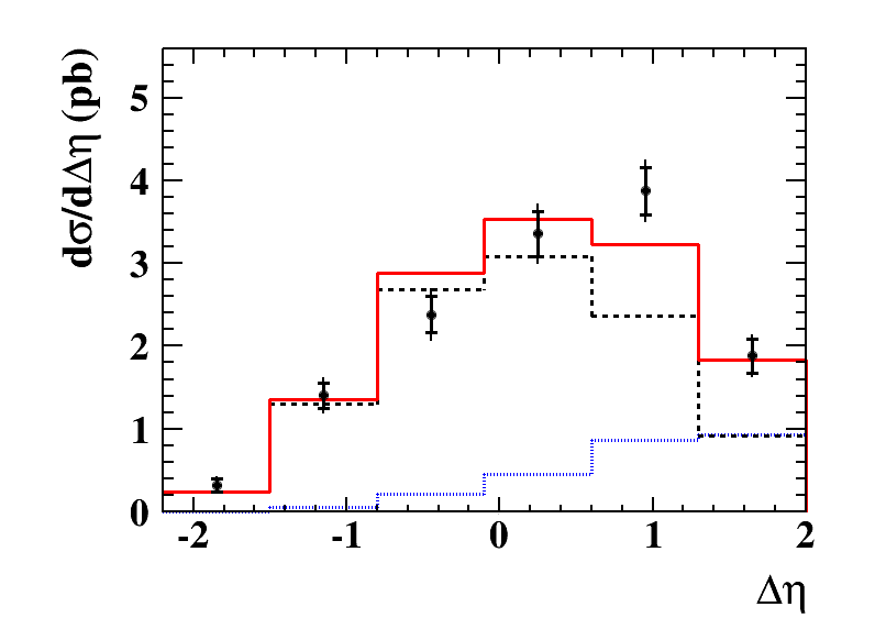
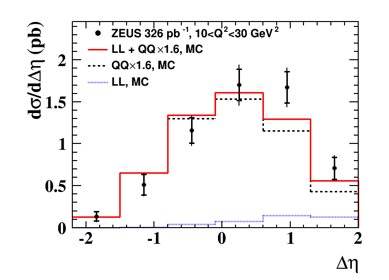
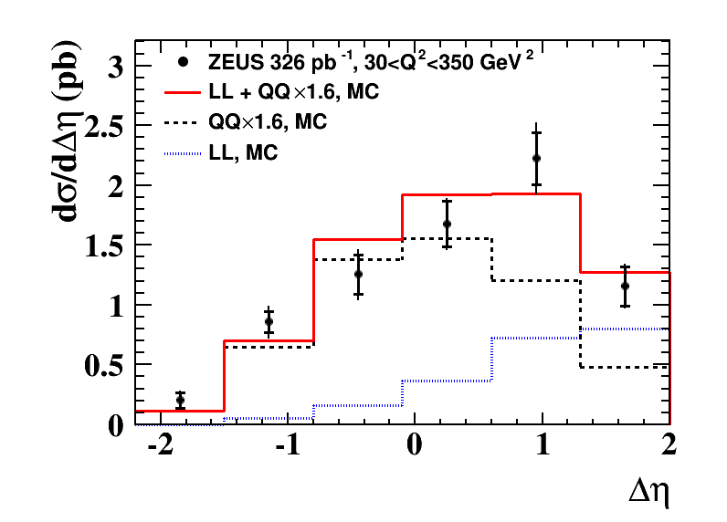
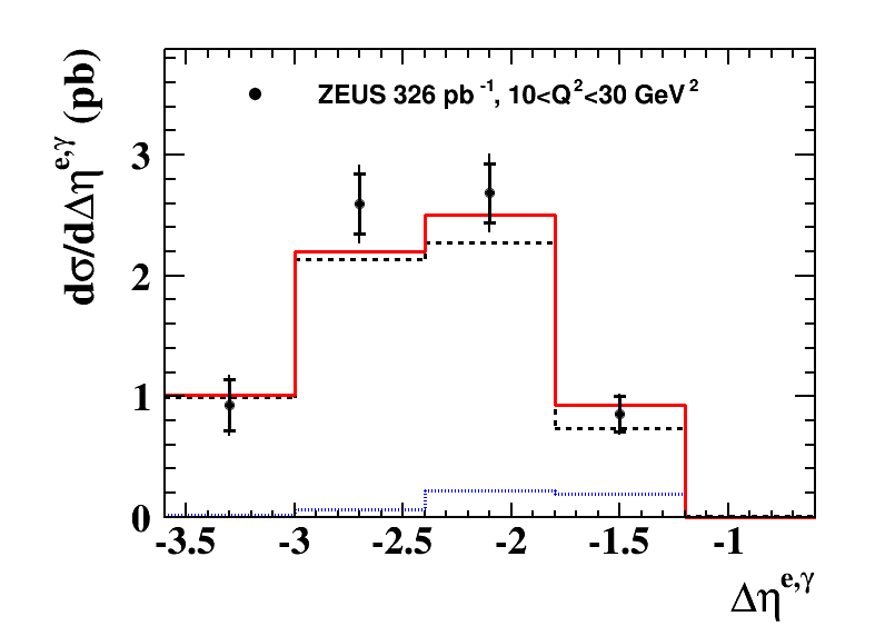
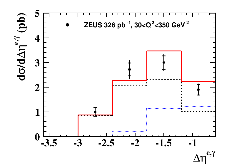
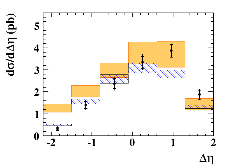
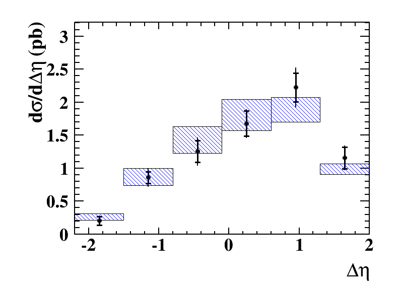
is the difference in pseudorapidity between the jet and the outgoing photon: , where and denote the pseudorapidity of the jet and the photon, respectively. This variable is sensitive to the dynamical properties of the scattering process;
-
•
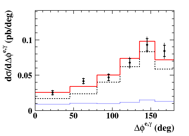
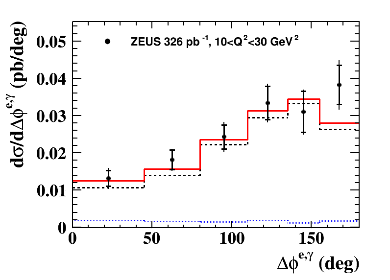
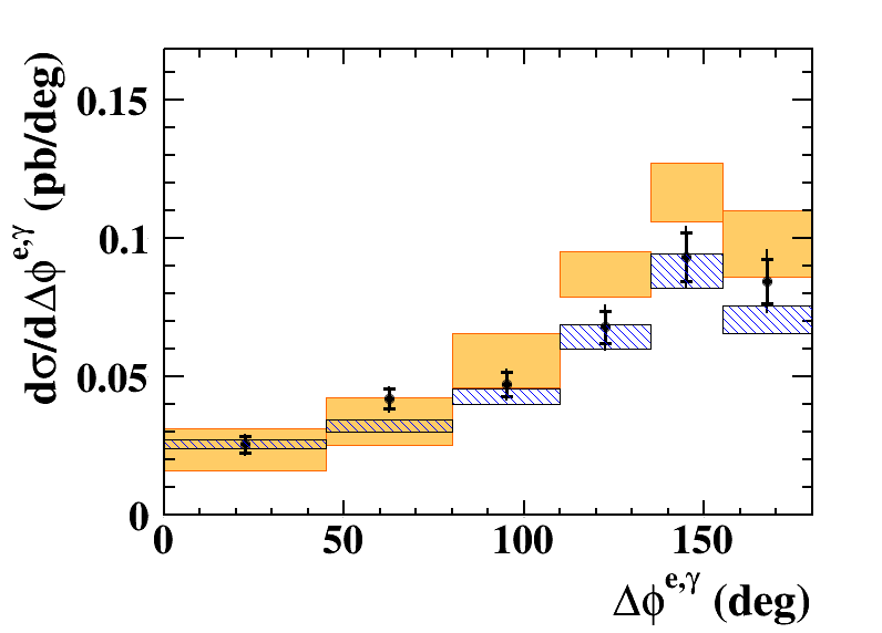
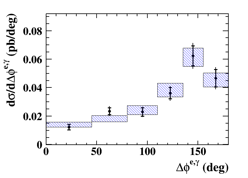
is the azimuthal angle between the scattered electron and the outgoing photon: , where denotes the azimuthal angle of the electron; this and the following variable are sensitive to higher-order processes and to whether the process is LL or QQ;
-
•
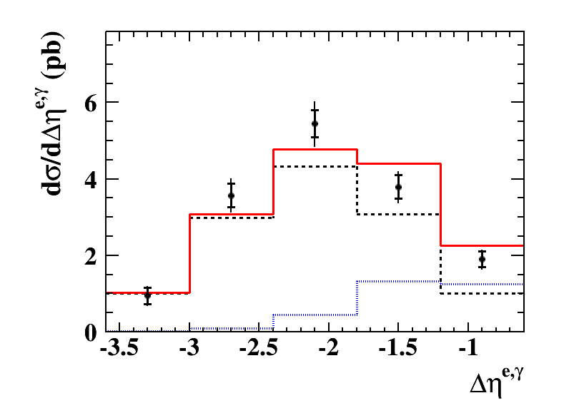
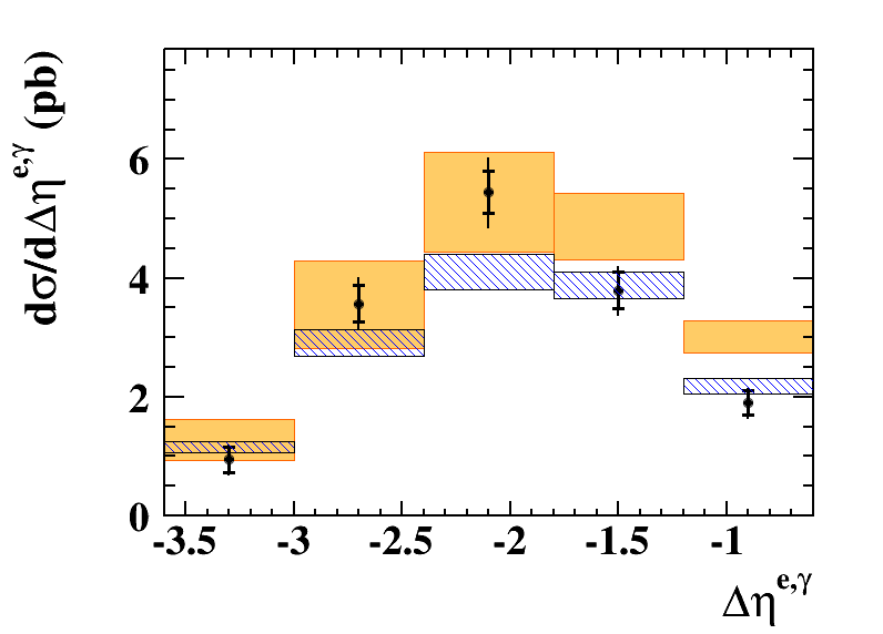
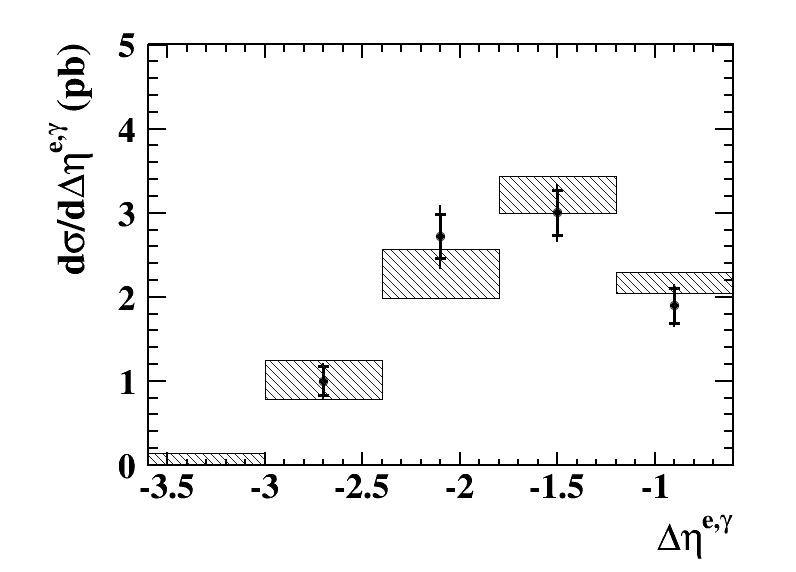
is the difference in pseudorapidity between the scattered electron and the photon: , where denotes the pseudorapidity of the electron.
A similar ZEUS analysis has been previously performed for photoproduction [44], studying all the present variables except those associated with the scattered electron.
5 Event simulation
Monte Carlo (MC) event samples were generated to evaluate the detector acceptance and to provide signal and background distributions. The program Pythia 6.416 [20] was used to simulate prompt-photon emission for the study of the event-reconstruction efficiency. In Pythia, this process is simulated as a DIS process with additional photon radiation from the quark line to account for QQ photons. Radiation from the lepton is not simulated.
The LL photons that were radiated into the detector and were isolated from the outgoing electron were simulated using the generator Djangoh 6 [47], an interface to the MC program Heracles 4.6.6 [48]; higher-order QCD effects were included using the colour dipole model of Ariadne 4.12 [49]. Hadronisation of the partonic final state was in each case performed by Jetset 7.4 [50] using the Lund string model [51]. Interference between the LL and QQ terms was neglected.
The main background to the QQ and LL photons came from photonic decays of neutral mesons produced in general DIS processes. This background was simulated using Djangoh 6, within the same framework as the LL events. This provided a realistic spectrum of single and multiple mesons with well modelled kinematic distributions.
The generated MC events were passed through ZEUS detector and trigger simulation programs based on Geant 3.21 [52]. They were then reconstructed and analysed by the same programs as the data.
6 Theoretical calculations
The Pythia predictions and the predictions of two parton-level models were compared to the results of the present analysis. The NLO QCD calculation of Aurenche, Fontannaz and Guillet (AFG) [21], was performed in the scheme. Uncertainties on the QCD scale at this order contribute a normalisation uncertainty of typically . This calculation was performed in the centre-of-mass frame and transformed into the laboratory frame, which introduces uncertainties on the cross sections in some regions of the parameter space due to non-perturbative effects [22]. The AFG predictions were calculated with a cut of 2.5 GeV on the photon transverse momentum in the centre-of-mass frame, and do not include an LL contribution, which was evaluated using the Djangoh–Heracles simulation and added separately to the AFG calculation for comparison with the data. The uncertainties on the AFG predictions shown in the present paper represent the QCD scale uncertainties.
A calculation by Baranov, Lipatov and Zotov (BLZ) [23] used updated parameters for the present paper. It is based on the -factorisation method. This approach uses unintegrated parton densities and takes into account both QQ and LL photons, neglecting the small interference contribution. The final result is obtained as the convolution of the off-shell scattering matrix element with the unintegrated quark distribution in the proton. In the -factorisation theory, some part of the final-state jets can originate not only from the hard subprocess but also from the parton evolution cascade in the initial state. The quoted uncertainties on the BLZ predictions represent the QCD scale uncertainties.
In the previous ZEUS analysis of prompt photons in DIS, the measured variables were associated with the entire event, with the outgoing photon, and with jets. Comparisons were made to an earlier NLO QCD theory [53, 54, 55] and to BLZ. Both theories described the shapes of the single-particle cross sections well, but failed to reproduce the normalisation of the data. A later version of the original AFG calculation agreed well with the results [56], and has been used in the present study.
The predictions of AFG and BLZ were calculated at the parton level and incorporated kinematic and isolation criteria corresponding to the data. Corrections to the hadron level were made using Pythia to determine the ratio of the hadron-level cross sections to those at the parton level for each variable in each bin. The Pythia events were weighted at the parton level to represent the shapes of the AFG and BLZ distributions in in order to calculate the hadronisation corrections for all the other measured variables. The corrections for AFG and BLZ were similar to within 10%. This procedure was also applied separately to the AFG predictions for the different ranges.
For the BLZ distribution, 98% of the parton-level cross section is in the (0.9, 1.0) bin; consequently, for this variable a transfer matrix from the parton to the hadron level was calculated using Pythia. The same procedure was used for the AFG distribution. The relevant transfer matrices for the other variables gave similar results to the reweighting procedure.
7 Extraction of the photon signal
The event sample selected according to the criteria described in Section 3 was dominated by background from neutral meson decays; thus the photon signal was extracted statistically following the approach used in previous ZEUS analyses [11, *pl:b472:175, *pl:b511:19, 16, 17].
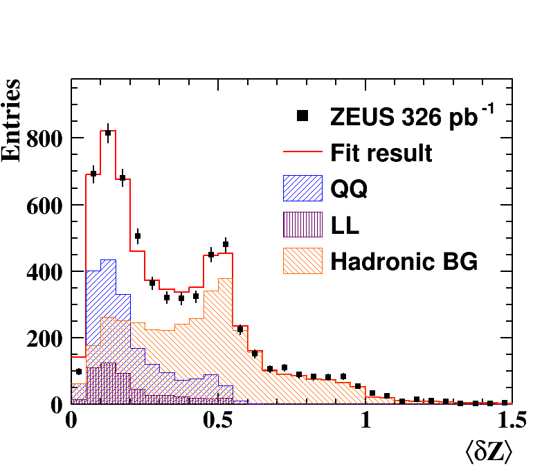
The photon signal was evaluated making use of the width of the BEMC energy-cluster corresponding to the photon candidate. This was calculated as the variable
where is the position of the centre of the -th cell, is the centroid of the EFO cluster, is the width of the cell in the direction, and is the energy recorded in the cell. The sum runs over all BEMC cells in the EFO.
The distributions of for the full data set and the fitted MC are shown in Fig. 2. The distribution exhibits a double-peaked structure with the first peak at , associated with the photon signal, and a second peak at , dominated by the background.
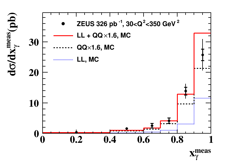
The contribution of isolated-photon events was determined for each bin in each measured variable by a fit to the distribution in the range , using the LL and QQ signal and background MC distributions as described in Section 5. The mean value of /n.d.f was 1.2. Compared to the earlier ZEUS publication [19], improvements have been made in the modelling of the shapes of the distributions of the QQ and LL contributions, using a comparison between the shapes associated with the scattered electron in MC simulation of DIS and in real data. By treating the LL and QQ photons separately, account is taken of the effect of their differing kinematic distributions on the acceptance, and the effect of their differing (, ) distributions on the shape of the photon signal.
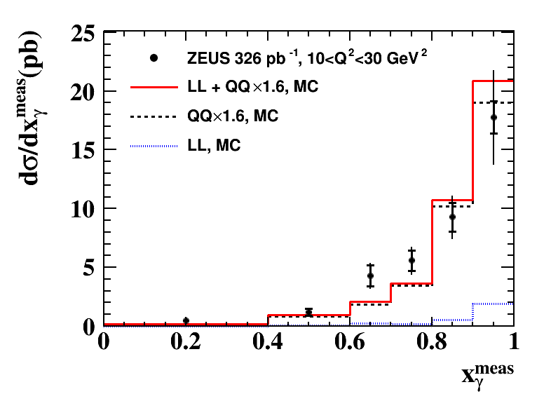
In performing the fit, the theoretically well determined LL contribution was kept constant at its MC-predicted value and the other components were varied. Of the 6149 events selected, correspond to the extracted signal, including 526 LL photons. The fitted scale factor applied to the QQ contribution in Fig. 2 was 1.6, consistent with the earlier ZEUS analysis.
For a given observable , the production cross section was determined for each bin using
where is the number of QQ photons extracted from the fit, is the bin width, is the total integrated luminosity, is the predicted cross section for LL photons from Djangoh–Heracles and is the acceptance correction for QQ photons. The value of was calculated, using the Pythia MC, from the ratio of the number of events generated to those reconstructed in a given bin; it lies in the range 0.91–2.28. To improve the representation of the data, and hence the accuracy of the acceptance corrections, the MC predictions were reweighted. This was done using parameterised functions of and of , and also bin-by-bin as a function of photon energy; the three reweighting factors were applied multiplicatively. Their net effect on the acceptances was small.
8 Systematic uncertainties
The sources of systematic uncertainty on the measured cross sections are as in the previous paper [19]. The principal sources of uncertainty were evaluated as follows:
-
•
the energy scale of the photon candidate was varied by . The mean change of the cross section was
-
•
the energy scale of the jets was varied by for jets with \GeV, for jets with in the range [6, 10] \GeV and for jets with \GeV. The uncertainty was typically ;
-
•
the energy scale of the scattered electron was varied by . The overall average effect on the cross sections was less than .
Systematic uncertainties related to the MC generators were evaluated as follows:
-
•
the dependence on the modelling of the hadronic background by means of Djangoh–Heracles was investigated by varying the upper limit for the fit in the range , giving variations that were typically
-
•
uncertainties in the acceptance due to the Pythia model were accounted for by taking half of the change attributable to the reweighting described in Section 7 as a systematic uncertainty; for most bins the effect was approximately .
Other sources of systematic uncertainty were found to be negligible and were ignored [57, 17]: these included variations on the cuts on , the track momentum, , and the electromagnetic fraction of the photon shower, and a variation of 5% on the LL fraction.
The systematic uncertainties were symmetrised by taking the mean of the positive and negative uncertainty values and were combined in quadrature. The common uncertainty of on the luminosity measurement is not included in the tables and figures.
9 Results
Differential cross sections for the production of an isolated photon in DIS with an additional jet have been measured in the laboratory frame in the kinematic region defined by GeV, , GeV and . The DIS electron was constrained to be in the angular range with energy greater than 10 GeV and GeV where was determined from the electron scattering angle. The jets were formed according to the -clustering algorithm with the parameter set to 1.0. Photon isolation was imposed such that at least of the energy of the jet-like object containing the photon belonged to the photon.
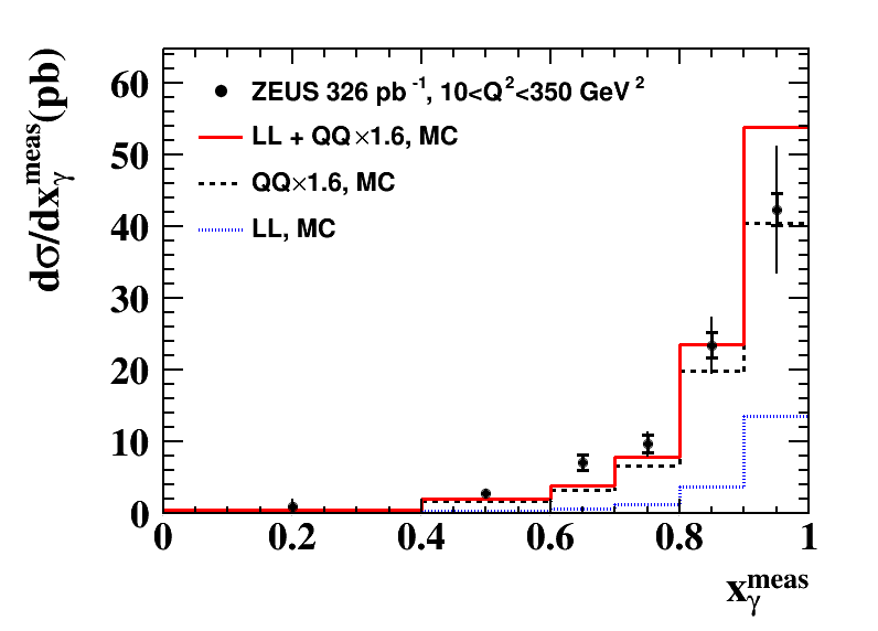
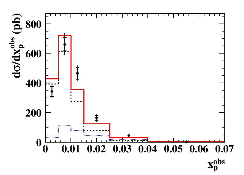
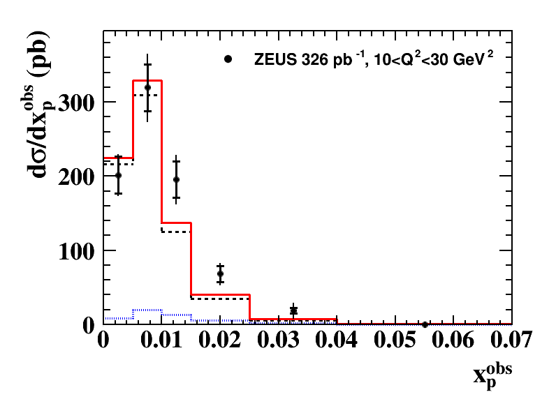
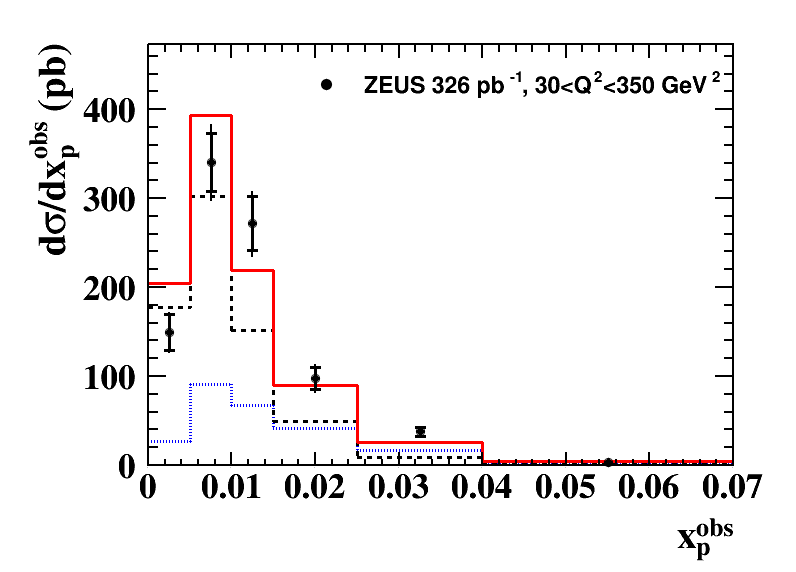
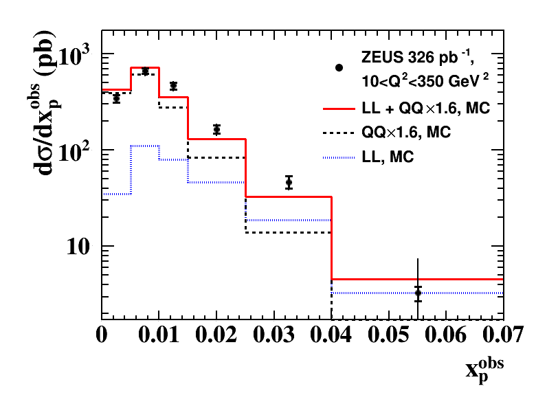
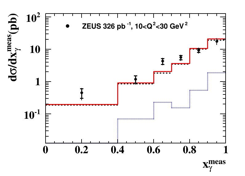
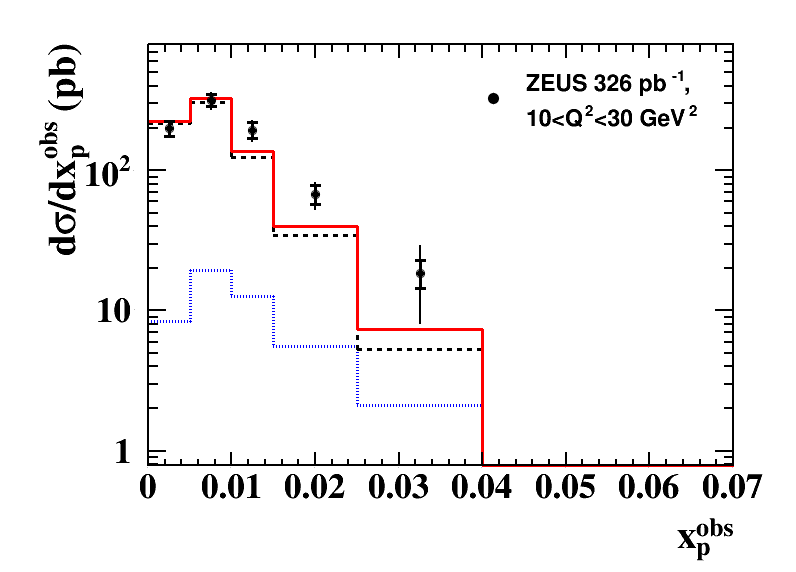
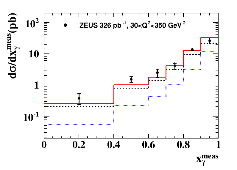
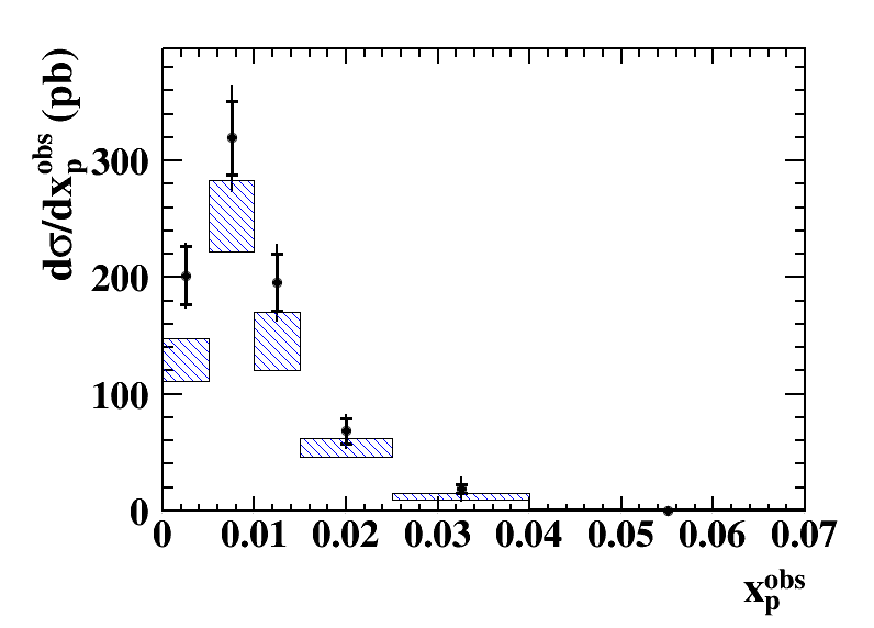
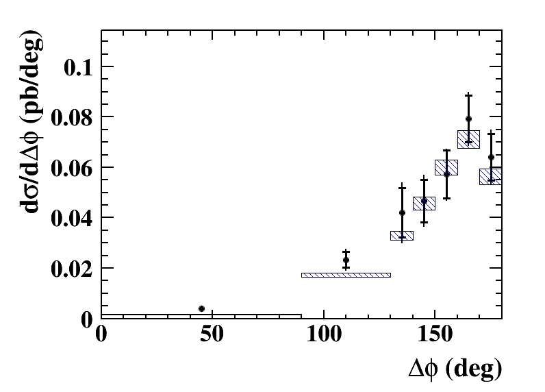
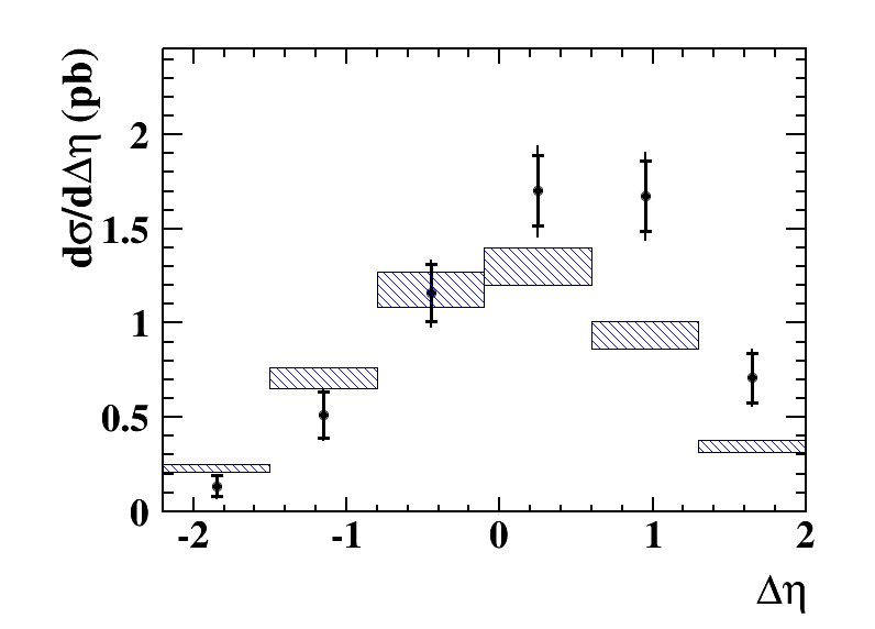
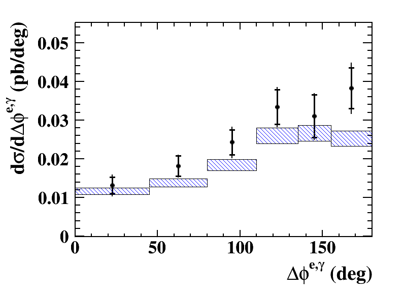
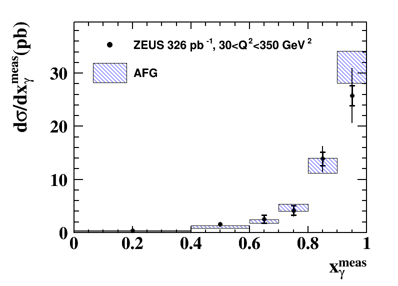
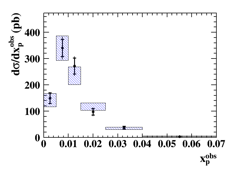
The differential cross sections for the full range as functions of and are shown in Fig. 3 and are given in Tables 1–6, which also list the values of the LL contributions and the hadronisation corrections. The cross section decreases with increasing , having a peak around 0.01, and rises at high values of and . The predictions for the sum of the expected LL contribution from Djangoh–Heracles and a factor of 1.6 times the expected QQ contribution from Pythia agree well with the measurements. The success of the Pythia calculation can be attributed to its use of a leading-logarithm approach to gluon emission to augment its LO parton-scattering calculation.
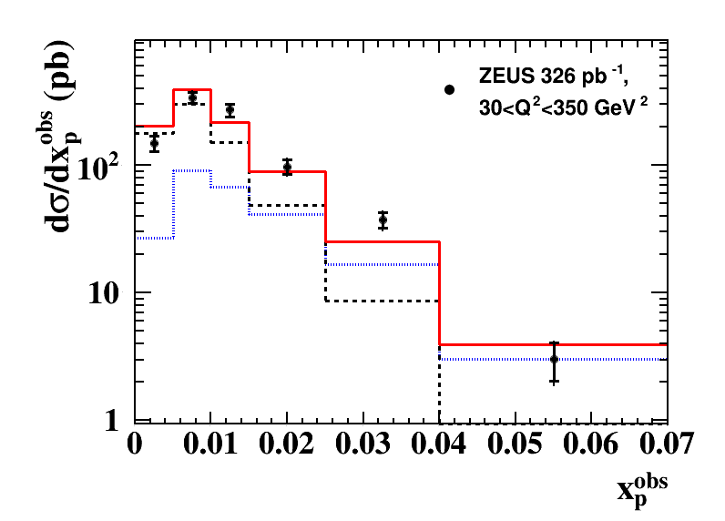
The differential cross sections for the separate ranges GeV2 and GeV2 are shown in Figs. 4 and 5. In both these ranges, a good description of the data is given by the combination of the LL and Pythia MCs. The LL contribution is small in the lower region, as was already seen in Fig. 3(a) of the earlier ZEUS publication [19]. In the higher range, the LL component contributes significantly, as can be seen in the , and distributions where it is dominant at high values of these variables. This reflects the changes with in the structure of the contributing processes.
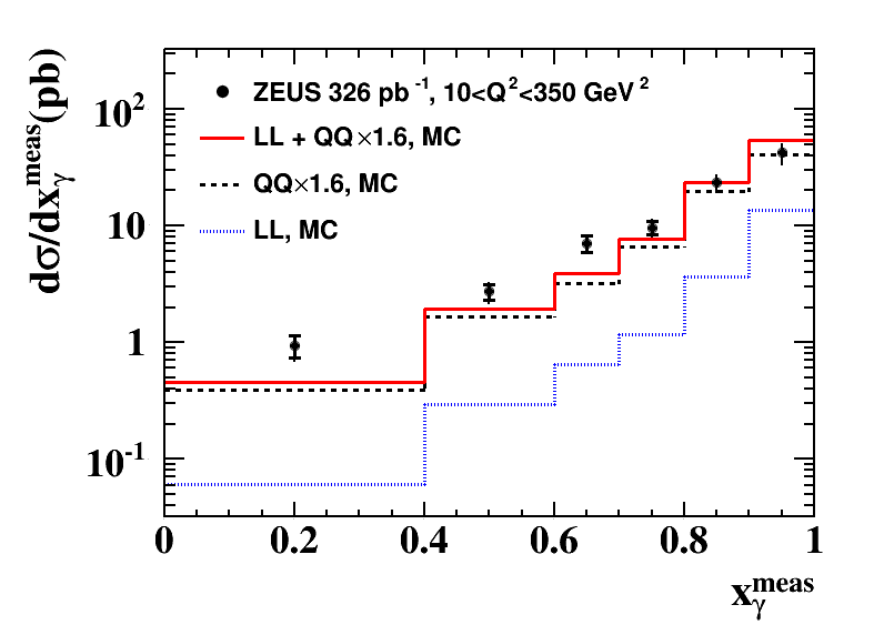
The increased importance of the LL component at higher is also reflected in the distribution. Figure 6 presents the and cross sections on a logarithmic scale. The data in the low- region are satisfactorily described by Pythia without the need for further higher-order processes.
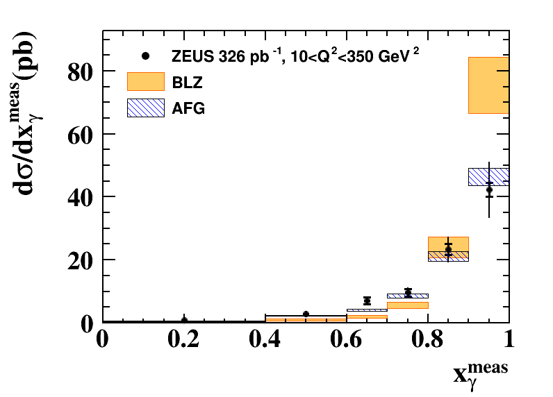
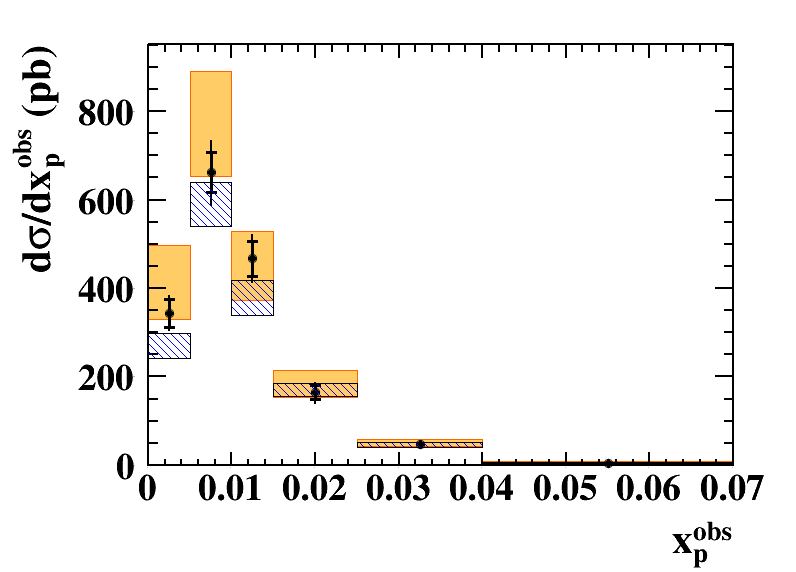
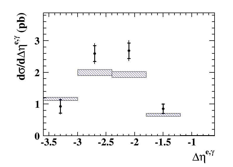
Comparisons of the data with the AFG and BLZ predictions are presented for the entire range in Fig. 7. The updated BLZ predictions describe the shape of most of the distributions reasonably well, but there is an overestimation of about 20% in the overall cross section, and the extremely peaked prediction for the distribution is not in agreement with the data. The AFG predictions describe all the distributions well and also agree in the overall normalisation.
Comparisons of the data with the AFG model in the two separate ranges are shown in Figs. 8–9. In the higher range, the description by AFG is excellent. In the lower range, the only deviation observable is in the distribution, where the data show a tendency towards higher values than the theory. This might be related to the cut of 2.5 GeV on the transverse photon momentum applied in the AFG calculation [21].
10 Summary
The production of isolated photons accompanied by jets has been measured in deep inelastic scattering with the ZEUS detector at HERA, using an integrated luminosity of . Expanding on earlier ZEUS results [19], which studied single-particle distributions, differential cross sections have been evaluated as functions of pairs of measured variables in combination. The kinematic region in the laboratory frame was defined by , , GeV and . The DIS electron was constrained to be in the angular range with energy greater than 10 GeV and GeV where was determined from the electron scattering angle. The jets were formed according to the -clustering algorithm with the parameter set to 1.0. Photon isolation was imposed such that at least of the energy of the jet-like object containing the photon belonged to the photon. Differential cross sections are presented for the following variables: the fraction of the incoming photon energy and momentum that is transferred to the outgoing photon and the leading jet; the fraction of the incoming proton energy transferred to the photon and leading jet; the differences in azimuthal angle and pseudorapidity between the outgoing photon and the leading jet and between the outgoing photon and the scattered electron.
The Pythia prediction for the quark-radiated photon component plus the Djangoh–Heracles calculation for the lepton-radiated component describes all the distributions well if the Pythia prediction is scaled up by a factor of 1.6. This is also true if the data are divided into ranges above and below a value of GeV2. Predictions from two theoretical models were also compared to the data. The BLZ model gives a fair description of the data but does not give a good description of the overall normalisation or the shape of some of the distributions. The AFG model gives an excellent description of the normalisation and almost all the distributions, both for the entire data set and for the separate ranges.
Acknowledgements
We appreciate the contributions to the construction and maintenance of the ZEUS detector of many people who are not listed as authors. The HERA machine group and the DESY computing staff are especially acknowledged for their success in providing excellent operation of the collider and the data-analysis environment. We thank the DESY directorate for their strong support and encouragement. We also thank P. Aurenche, M. Fontannaz and A. Lipatov for providing theoretical results and express our appreciation for the contributions from our much-missed late colleague, Nikolai Zotov.
10
References
- [1] E. Anassontzis et al., Z. Phys. C 13 (1982) 277
- [2] WA70 Collaboration, M. Bonesini et al., Z. Phys. C 38 (1988) 371
- [3] E706 Collaboration, G. Alverson et al., Phys. Rev. D 48 (1993) 5
-
[4]
CDF Collaboration, F. Abe et al.,
Phys. Rev. Lett. 73 (1994) 2662;
Erratum: Phys. Rev. Lett. 74 (1995) 1891 - [5] CDF Collaboration, D. Acosta et al., Phys. Rev. Lett. 95 (2005) 022003
- [6] DØ Collaboration, B. Abbott et al., Phys. Rev. Lett. 84 (2000) 2786
-
[7]
DØ Collaboration, V.M. Abazov et al.,
Phys. Lett. B 639 (2006) 151;
Erratum: Phys. Lett. B 658 (2008) 285 - [8] ATLAS Collaboration. M. Aaboud et al., Nucl. Phys. B 918 (2017) 257
- [9] ATLAS Collaboration. M. Aaboud et al., Phys. Lett. B 770 (2017) 473
- [10] CMS Collaboration. S. Chatrchyan et al., JHEP 06 (2014) 009
- [11] ZEUS Collaboration, J. Breitweg et al., Phys. Lett. B 413 (1997) 201
- [12] ZEUS Collaboration, J. Breitweg et al., Phys. Lett. B 472 (2000) 175
- [13] ZEUS Collaboration, S. Chekanov et al., Phys. Lett. B 511 (2001) 19
- [14] ZEUS Collaboration, S Chekanov et al., Eur. Phys. J. C 49 (2007) 511
- [15] H1 Collaboration, A. Aktas et al., Eur. Phys. J. C 38 (2004) 437
- [16] ZEUS Collaboration, S. Chekanov et al., Phys. Lett. B 595 (2004) 86
- [17] ZEUS Collaboration, S. Chekanov et al., Phys. Lett. B 687 (2010) 16
- [18] H1 Collaboration, F.D. Aaron et al., Eur. Phys. J. C 54 (2008) 371
- [19] ZEUS Collaboration, H. Abramowicz et al., Phys. Lett. B 715 (2012) 88
- [20] T. Sjöstrand et al., JHEP 0605 (2006) 26
- [21] P. Aurenche, M. Fontannaz and J.Ph. Guillet, Eur. Phys. J. C 44 (2005) 395
- [22] P. Aurenche and M. Fontannaz, Eur. Phys. J. C 77 (2017) 324
- [23] S. Baranov, A. Lipatov and N. Zotov, Phys. Rev. D 81 (2010) 094034
-
[24]
ZEUS Collaboration, U. Holm (ed.),
The ZEUS Detector.
Status Report (unpublished), DESY (1993),
available on http://www-zeus.desy.de/bluebook/bluebook.html - [25] N. Harnew et al., Nucl. Inst. Meth. A 279 (1989) 290
- [26] B. Foster et al., Nucl. Phys. Proc. Suppl. B 32 (1993) 181
- [27] B. Foster et al., Nucl. Inst. Meth. A 338 (1994) 254
- [28] A. Polini et al., Nucl. Inst. Meth. A 581 (2007) 656
- [29] M. Derrick et al., Nucl. Inst. Meth. A 309 (1991) 77
- [30] A. Andresen et al., Nucl. Inst. Meth. A 309 (1991) 101
- [31] A. Caldwell et al., Nucl. Inst. Meth. A 321 (1992) 356
- [32] A. Bernstein et al., Nucl. Inst. Meth. A 336 (1993) 23
- [33] J. Andruszków et al., Preprint DESY-92-066, DESY, 1992
- [34] ZEUS Collaboration, M. Derrick et al., Z. Phys. C 63 (1994) 391
- [35] J. Andruszków et al., Acta Phys. Pol. B 32 (2001) 2025
- [36] M. Helbich et al., Nucl. Inst. Meth. A 565 (2006) 572
- [37] W.H. Smith, K. Tokushuku and L.W. Wiggers, Proc. Computing in High-Energy Physics (CHEP), Annecy, France, Sept. 1992, C. Verkerk and W. Wojcik (eds.), p. 222. CERN, Geneva, Switzerland (1992). Also in preprint DESY 92-150B
- [38] P. Allfrey et al., Nucl. Inst. Meth. A 580 (2007) 1257
- [39] H. Abramowicz, A. Caldwell and R. Sinkus, Nucl. Inst. Meth. A 365 (1995) 508
- [40] ZEUS Collaboration, M. Derrick et al., Phys. Lett. B 303 (1993) 183
- [41] ZEUS Collaboration, J. Breitweg et al., Eur. Phys. J. C 1 (1998) 81
- [42] ZEUS Collaboration, J. Breitweg et al., Eur. Phys. J. C 6 (1999) 43
- [43] G.M. Briskin, Ph.D. Thesis, Tel Aviv University (1998) DESY-THESIS-1998-036
- [44] ZEUS Collaboration, H. Abramowicz et al., JHEP 08 (2014) 23
- [45] S. Catani et al., Nucl. Phys. B 406 (1993) 187
- [46] S.D. Ellis and D.E. Soper, Phys. Rev. D 48 (1993) 3160
- [47] H. Spiesberger (1998) HERACLES and DJANGOH Event Generators for ep Interactions at HERA Including Radiative Processes (1998) http://www.thep.physik,uni-mainz.de/~hspies/djangoh/djangoh.html
- [48] A. Kwiatkowski, H. Spiesberger and H.-J. Möhring, Comp. Phys. Comm. 69 (1992) 155
- [49] L. Lönnblad, Comp. Phys. Comm. 71 (1992) 15
- [50] T. Sjöstrand, Comp. Phys. Comm. 39 (1986) 347
- [51] B. Andersson et al., Phys. Rept. 97 (1983) 31
- [52] R. Brun et al., geant3, Technical Report CERN-DD/EE/84-1, CERN (1987)
- [53] A. Gehrmann-De Ridder, G. Kramer and H. Spiesberger, Nucl. Phys. B 578 (2000) 326
- [54] A. Gehrmann-De Ridder, T. Gehrmann and E. Poulsen, Phys. Rev. Lett. 96 (2006) 132002
- [55] A. Gehrmann-De Ridder, T. Gehrmann and E. Poulsen, Eur. Phys. J. C 47 (2006) 395
- [56] P. Aurenche and M. Fontannaz, Eur. Phys. J. C 75 (2015) 64
-
[57]
M. Forrest,
Ph.D. Thesis, University of Glasgow (2010),
http://theses.gla.ac.uk/1761/
|
() | () |
|
||||||||
| GeV2 | |||||||||||
| 0.0 – | 0.4 | 0.94 | 0.20 (stat.) | 0.11 (sys.) | 0.06 | 0.01 (stat.) | 0.63 | ||||
| 0.4 – | 0.6 | 2.73 | 0.43 (stat.) | 0.32 (sys.) | 0.29 | 0.04 (stat.) | 0.90 | ||||
| 0.6 – | 0.7 | 7.06 | 1.14 (stat.) | 0.38 (sys.) | 0.65 | 0.09 (stat.) | 1.27 | ||||
| 0.7 – | 0.8 | 9.64 | 1.24 (stat.) | 1.06 (sys.) | 1.17 | 0.12 (stat.) | 1.93 | ||||
| 0.8 – | 0.9 | 23.40 | 1.75 (stat.) | 3.51 (sys.) | 3.67 | 0.22 (stat.) | 2.06 | ||||
| 0.9 – | 1.0 | 42.34 | 2.26 (stat.) | 8.54 (sys.) | 13.49 | 0.42 (stat.) | 0.64 | ||||
| GeV2 | |||||||||||
| 0.0 – | 0.4 | 0.45 | 0.15 (stat.) | 0.09 (sys.) | 0.01 | 0.01 (stat.) | 0.68 | ||||
| 0.4 – | 0.6 | 1.19 | 0.31 (stat.) | 0.18 (sys.) | 0.07 | 0.02 (stat.) | 1.00 | ||||
| 0.6 – | 0.7 | 4.30 | 0.88 (stat.) | 0.49 (sys.) | 0.23 | 0.06 (stat.) | 1.30 | ||||
| 0.7 – | 0.8 | 5.58 | 0.88 (stat.) | 0.69 (sys.) | 0.16 | 0.04 (stat.) | 2.02 | ||||
| 0.8 – | 0.9 | 9.27 | 1.20 (stat.) | 1.32 (sys.) | 0.54 | 0.08 (stat.) | 2.11 | ||||
| 0.9 – | 1.0 | 17.76 | 1.37 (stat.) | 3.73 (sys.) | 1.89 | 0.16 (stat.) | 0.63 | ||||
| GeV2 | |||||||||||
| 0.0 – | 0.4 | 0.38 | 0.15 (stat.) | 0.05 (sys.) | 0.06 | 0.01 (stat.) | 0.60 | ||||
| 0.4 – | 0.6 | 1.55 | 0.30 (stat.) | 0.23 (sys.) | 0.22 | 0.04 (stat.) | 0.82 | ||||
| 0.6 – | 0.7 | 2.50 | 0.73 (stat.) | 0.36 (sys.) | 0.42 | 0.07 (stat.) | 1.25 | ||||
| 0.7 – | 0.8 | 4.15 | 0.89 (stat.) | 0.53 (sys.) | 1.01 | 0.11 (stat.) | 1.86 | ||||
| 0.8 – | 0.9 | 13.90 | 1.27 (stat.) | 2.01 (sys.) | 3.14 | 0.20 (stat.) | 2.02 | ||||
| 0.9 – | 1.0 | 25.81 | 1.89 (stat.) | 4.74 (sys.) | 11.61 | 0.38 (stat.) | 0.65 | ||||
|
() | () |
|
||||||||
| GeV2 | |||||||||||
| 0.000 – | 0.005 | 344.3 | 31.7 (stat.) | 22.9 (sys.) | 35.2 | 3.0 (stat.) | 0.69 | ||||
| 0.005 – | 0.010 | 661.8 | 45.3 (stat.) | 56.6 (sys.) | 110.8 | 5.3 (stat.) | 0.81 | ||||
| 0.010 – | 0.015 | 467.1 | 38.9 (stat.) | 35.5 (sys.) | 80.0 | 4.5 (stat.) | 0.91 | ||||
| 0.015 – | 0.025 | 164.5 | 16.5 (stat.) | 16.1 (sys.) | 46.6 | 2.4 (stat.) | 0.99 | ||||
| 0.025 – | 0.040 | 46.7 | 6.8 (stat.) | 2.7 (sys.) | 18.7 | 1.3 (stat.) | 1.06 | ||||
| 0.040 – | 0.070 | 3.3 | 0.6 (stat.) | 2.1 (sys.) | 3.3 | 0.4 (stat.) | 1.00 | ||||
| GeV2 | |||||||||||
| 0.000 – | 0.005 | 201.8 | 25.0 (stat.) | 11.1 (sys.) | 8.4 | 1.4 (stat.) | 0.71 | ||||
| 0.005 – | 0.010 | 319.6 | 31.4 (stat.) | 31.8 (sys.) | 19.4 | 2.2 (stat.) | 0.84 | ||||
| 0.010 – | 0.015 | 195.5 | 24.5 (stat.) | 20.5 (sys.) | 12.7 | 1.8 (stat.) | 0.98 | ||||
| 0.015 – | 0.025 | 68.1 | 10.4 (stat.) | 9.8 (sys.) | 5.6 | 0.9 (stat.) | 1.03 | ||||
| 0.025 – | 0.040 | 18.7 | 4.1 (stat.) | 9.5 (sys.) | 2.1 | 0.4 (stat.) | 1.08 | ||||
| 0.040 – | 0.070 | 0.2 | 0.1 (stat.) | 0.1 (sys.) | 0.2 | 0.1 (stat.) | 0.95 | ||||
| GeV2 | |||||||||||
| 0.000 – | 0.005 | 149.3 | 20.0 (stat.) | 9.1 (sys.) | 26.8 | 2.6 (stat.) | 0.68 | ||||
| 0.005 – | 0.010 | 340.7 | 32.9 (stat.) | 25.0 (sys.) | 91.4 | 4.8 (stat.) | 0.78 | ||||
| 0.010 – | 0.015 | 271.7 | 30.5 (stat.) | 17.4 (sys.) | 67.3 | 4.1 (stat.) | 0.88 | ||||
| 0.015 – | 0.025 | 97.7 | 12.8 (stat.) | 8.1 (sys.) | 41.0 | 2.3 (stat.) | 0.97 | ||||
| 0.025 – | 0.040 | 37.5 | 5.3 (stat.) | 3.1 (sys.) | 16.6 | 1.2 (stat.) | 1.06 | ||||
| 0.040 – | 0.070 | 3.0 | 1.0 (stat.) | 2.1 (sys.) | 3.0 | 0.4 (stat.) | 1.01 | ||||
|
() | () |
|
|||||||||
| GeV2 | ||||||||||||
| 0 – | 90 | 0.020 | 0.002 (stat.) | 0.003 (sys.) | 0.004 | 0.001 (stat.) | 0.68 | |||||
| 90 – | 130 | 0.063 | 0.005 (stat.) | 0.005 (sys.) | 0.012 | 0.001 (stat.) | 0.82 | |||||
| 130 – | 140 | 0.093 | 0.012 (stat.) | 0.008 (sys.) | 0.017 | 0.002 (stat.) | 0.88 | |||||
| 140 – | 150 | 0.080 | 0.012 (stat.) | 0.007 (sys.) | 0.021 | 0.002 (stat.) | 0.92 | |||||
| 150 – | 160 | 0.117 | 0.013 (stat.) | 0.006 (sys.) | 0.021 | 0.002 (stat.) | 0.95 | |||||
| 160 – | 170 | 0.129 | 0.011 (stat.) | 0.005 (sys.) | 0.027 | 0.002 (stat.) | 0.95 | |||||
| 170 – | 180 | 0.108 | 0.012 (stat.) | 0.007 (sys.) | 0.026 | 0.002 (stat.) | 0.94 | |||||
| GeV2 | ||||||||||||
| 0 – | 90 | 0.004 | 0.001 (stat.) | 0.001 (sys.) | 0.000 | 0.001 (stat.) | 0.68 | |||||
| 90 – | 130 | 0.023 | 0.003 (stat.) | 0.002 (sys.) | 0.001 | 0.001 (stat.) | 0.78 | |||||
| 130 – | 140 | 0.042 | 0.010 (stat.) | 0.007 (sys.) | 0.003 | 0.001 (stat.) | 0.79 | |||||
| 140 – | 150 | 0.047 | 0.009 (stat.) | 0.005 (sys.) | 0.004 | 0.001 (stat.) | 0.85 | |||||
| 150 – | 160 | 0.057 | 0.010 (stat.) | 0.003 (sys.) | 0.005 | 0.001 (stat.) | 0.91 | |||||
| 160 – | 170 | 0.079 | 0.009 (stat.) | 0.004 (sys.) | 0.007 | 0.001 (stat.) | 0.93 | |||||
| 170 – | 180 | 0.064 | 0.009 (stat.) | 0.005 (sys.) | 0.007 | 0.001 (stat.) | 0.93 | |||||
| GeV2 | ||||||||||||
| 0 – | 90 | 0.015 | 0.002 (stat.) | 0.002 (sys.) | 0.004 | 0.001 (stat.) | 0.68 | |||||
| 90 – | 130 | 0.040 | 0.004 (stat.) | 0.003 (sys.) | 0.011 | 0.001 (stat.) | 0.83 | |||||
| 130 – | 140 | 0.049 | 0.008 (stat.) | 0.002 (sys.) | 0.014 | 0.001 (stat.) | 0.96 | |||||
| 140 – | 150 | 0.030 | 0.008 (stat.) | 0.001 (sys.) | 0.017 | 0.002 (stat.) | 0.99 | |||||
| 150 – | 160 | 0.064 | 0.009 (stat.) | 0.007 (sys.) | 0.016 | 0.001 (stat.) | 1.01 | |||||
| 160 – | 170 | 0.046 | 0.007 (stat.) | 0.005 (sys.) | 0.020 | 0.002 (stat.) | 1.01 | |||||
| 170 – | 180 | 0.045 | 0.009 (stat.) | 0.003 (sys.) | 0.019 | 0.002 (stat.) | 0.97 | |||||
|
() | () |
|
||||||||
| GeV2 | |||||||||||
| –2.2 – | –1.5 | 0.32 | 0.08 (stat.) | 0.05 (sys.) | 0.01 | 0.01 (stat.) | 0.76 | ||||
| –1.5 – | –0.8 | 1.41 | 0.15 (stat.) | 0.14 (sys.) | 0.06 | 0.01 (stat.) | 0.66 | ||||
| –0.8 – | –0.1 | 2.38 | 0.22 (stat.) | 0.21 (sys.) | 0.21 | 0.02 (stat.) | 0.74 | ||||
| –0.1 – | 0.6 | 3.36 | 0.27 (stat.) | 0.23 (sys.) | 0.45 | 0.03 (stat.) | 0.87 | ||||
| 0.6 – | 1.3 | 3.88 | 0.28 (stat.) | 0.22 (sys.) | 0.87 | 0.04 (stat.) | 1.04 | ||||
| 1.3 – | 2.0 | 1.88 | 0.21 (stat.) | 0.12 (sys.) | 0.92 | 0.04 (stat.) | 1.11 | ||||
| GeV2 | |||||||||||
| –2.2 – | –1.5 | 0.14 | 0.05 (stat.) | 0.03 (sys.) | 0.00 | 0.01 (stat.) | 0.63 | ||||
| –1.5 – | –0.8 | 0.51 | 0.12 (stat.) | 0.04 (sys.) | 0.00 | 0.01 (stat.) | 0.68 | ||||
| –0.8 – | –0.1 | 1.16 | 0.15 (stat.) | 0.09 (sys.) | 0.04 | 0.01 (stat.) | 0.77 | ||||
| –0.1 – | 0.6 | 1.70 | 0.19 (stat.) | 0.15 (sys.) | 0.08 | 0.01 (stat.) | 0.90 | ||||
| 0.6 – | 1.3 | 1.67 | 0.19 (stat.) | 0.13 (sys.) | 0.14 | 0.02 (stat.) | 1.08 | ||||
| 1.3 – | 2.0 | 0.71 | 0.13 (stat.) | 0.07 (sys.) | 0.13 | 0.02 (stat.) | 1.07 | ||||
| GeV2 | |||||||||||
| –2.2 – | –1.5 | 0.20 | 0.07 (stat.) | 0.03 (sys.) | 0.00 | 0.01 (stat.) | 0.83 | ||||
| –1.5 – | –0.8 | 0.86 | 0.09 (stat.) | 0.09 (sys.) | 0.05 | 0.01 (stat.) | 0.65 | ||||
| –0.8 – | –0.1 | 1.25 | 0.16 (stat.) | 0.13 (sys.) | 0.16 | 0.02 (stat.) | 0.72 | ||||
| –0.1 – | 0.6 | 1.68 | 0.19 (stat.) | 0.08 (sys.) | 0.37 | 0.03 (stat.) | 0.85 | ||||
| 0.6 – | 1.3 | 2.23 | 0.22 (stat.) | 0.19 (sys.) | 0.72 | 0.04 (stat.) | 1.02 | ||||
| 1.3 – | 2.0 | 1.16 | 0.16 (stat.) | 0.06 (sys.) | 0.80 | 0.04 (stat.) | 1.14 | ||||
|
) | ) |
|
|||||||||
| GeV2 | ||||||||||||
| 0 – | 45 | 0.025 | 0.003 (stat.) | 0.002 (sys.) | 0.009 | 0.001 (stat.) | 0.95 | |||||
| 45 – | 80 | 0.042 | 0.004 (stat.) | 0.003 (sys.) | 0.010 | 0.001 (stat.) | 0.94 | |||||
| 80 – | 110 | 0.047 | 0.004 (stat.) | 0.003 (sys.) | 0.010 | 0.001 (stat.) | 0.92 | |||||
| 110 – | 135 | 0.068 | 0.006 (stat.) | 0.006 (sys.) | 0.012 | 0.001 (stat.) | 0.85 | |||||
| 135 – | 155 | 0.093 | 0.009 (stat.) | 0.007 (sys.) | 0.015 | 0.001 (stat.) | 0.79 | |||||
| 155 – | 180 | 0.085 | 0.008 (stat.) | 0.008 (sys.) | 0.013 | 0.001 (stat.) | 0.73 | |||||
| GeV2 | ||||||||||||
| 0 – | 45 | 0.013 | 0.002 (stat.) | 0.002 (sys.) | 0.002 | 0.001 (stat.) | 0.95 | |||||
| 45 – | 80 | 0.018 | 0.003 (stat.) | 0.001 (sys.) | 0.002 | 0.001 (stat.) | 0.94 | |||||
| 80 – | 110 | 0.024 | 0.003 (stat.) | 0.002 (sys.) | 0.001 | 0.001 (stat.) | 0.91 | |||||
| 110 – | 135 | 0.033 | 0.005 (stat.) | 0.002 (sys.) | 0.002 | 0.001 (stat.) | 0.85 | |||||
| 135 – | 155 | 0.031 | 0.006 (stat.) | 0.002 (sys.) | 0.001 | 0.001 (stat.) | 0.78 | |||||
| 155 – | 180 | 0.038 | 0.005 (stat.) | 0.004 (sys.) | 0.002 | 0.001 (stat.) | 0.80 | |||||
| GeV2 | ||||||||||||
| 0 – | 45 | 0.012 | 0.002 (stat.) | 0.001 (sys.) | 0.007 | 0.001 (stat.) | 0.95 | |||||
| 45 – | 80 | 0.024 | 0.002 (stat.) | 0.002 (sys.) | 0.009 | 0.001 (stat.) | 0.95 | |||||
| 80 – | 110 | 0.023 | 0.003 (stat.) | 0.002 (sys.) | 0.009 | 0.001 (stat.) | 0.93 | |||||
| 110 – | 135 | 0.036 | 0.004 (stat.) | 0.003 (sys.) | 0.010 | 0.001 (stat.) | 0.86 | |||||
| 135 – | 155 | 0.063 | 0.007 (stat.) | 0.005 (sys.) | 0.014 | 0.001 (stat.) | 0.80 | |||||
| 155 – | 180 | 0.047 | 0.006 (stat.) | 0.004 (sys.) | 0.011 | 0.001 (stat.) | 0.70 | |||||
|
) | ) |
|
||||||||
| GeV2 | |||||||||||
| –3.6 – | –3.0 | 0.94 | 0.21 (stat.) | 0.12 (sys.) | 0.02 | 0.01 (stat.) | 0.80 | ||||
| –3.0 – | –2.4 | 3.57 | 0.30 (stat.) | 0.30 (sys.) | 0.08 | 0.01 (stat.) | 0.82 | ||||
| –2.4 – | –1.8 | 5.44 | 0.36 (stat.) | 0.45 (sys.) | 0.45 | 0.03 (stat.) | 0.83 | ||||
| –1.8 – | –1.2 | 3.79 | 0.31 (stat.) | 0.26 (sys.) | 1.33 | 0.05 (stat.) | 0.85 | ||||
| –1.2 – | –0.6 | 1.90 | 0.21 (stat.) | 0.11 (sys.) | 1.24 | 0.05 (stat.) | 0.89 | ||||
| GeV2 | |||||||||||
| –3.6 – | –3.0 | 0.93 | 0.21 (stat.) | 0.12 (sys.) | 0.02 | 0.01 (stat.) | 0.81 | ||||
| –3.0 – | –2.4 | 2.60 | 0.25 (stat.) | 0.19 (sys.) | 0.06 | 0.01 (stat.) | 0.85 | ||||
| –2.4 – | –1.8 | 2.69 | 0.25 (stat.) | 0.19 (sys.) | 0.22 | 0.02 (stat.) | 0.89 | ||||
| –1.8 – | –1.2 | 0.86 | 0.15 (stat.) | 0.07 (sys.) | 0.19 | 0.02 (stat.) | 0.92 | ||||
| GeV2 | |||||||||||
| –3.0 – | –2.4 | 1.00 | 0.17 (stat.) | 0.11 (sys.) | 0.02 | 0.01 (stat.) | 0.77 | ||||
| –2.4 – | –1.8 | 2.72 | 0.26 (stat.) | 0.25 (sys.) | 0.23 | 0.02 (stat.) | 0.80 | ||||
| –1.8 – | –1.2 | 3.00 | 0.27 (stat.) | 0.18 (sys.) | 1.14 | 0.05 (stat.) | 0.84 | ||||
| –1.2 – | -0.6 | 1.90 | 0.21 (stat.) | 0.11 (sys.) | 1.24 | 0.05 (stat.) | 0.89 | ||||


(a) (b)


(c) (d)
ZEUS
(a) (b)
(c) (d)
(e) (f)
ZEUS
(a) (b)
(c) (d)
(e) (f)
ZEUS
(a) (b)
(c) (d)
(e) (f)
ZEUS
(a) (b)
(c) (d)
(e) (f)
ZEUS
(a) (b)
(c) (d)
(e) (f)
ZEUS
(a) (b)
(c) (d)
(e) (f)
ZEUS
(a) (b)
(e) (f)
(c) (d)