Abstract

This article is concerned with three heteroclinic cycles forming a heteroclinic network in ${\mathbb{R}}^{6}$. The stability of the cycles and of the network are studied. The cycles are of a type that has not been studied before, and provide an illustration for the difficulties arising in dealing with cycles and networks in high dimension. In order to obtain information on the stability for the present network and cycles, in addition to the information on eigenvalues and transition matrices, it is necessary to perform a detailed geometric analysis of return maps. Some general results and tools for this type of analysis are also developed here.

1 Introduction

In this article we derive stability conditions for a specific heteroclinic network in ${\mathbb{R}}^{6}$, as well as for its cycles. This network is of a type that has not been studied before and has features that distinguish it clearly from what is discussed in the literature. This case study both provides a starting point for further general stability results and illustrates the difficulties arising in the study of higher-dimensional more general networks.

Recall that the smallest dimension where a robust heteroclinic cycle can exist is $n=3$. Robust heteroclinic cycles existing in ${\mathbb{R}}^{3}$ have been known for a long time, going as far back as the work of dos Reis [22] and Guckenheimer and Holmes [8]; the list of possible cycles is short. In ${\mathbb{R}}^{4}$ the situation becomes more complex. However, general results on heteroclinic cycles and networks in ${\mathbb{R}}^{4}$ are known in the literature, starting with that by Krupa and Melbourne [11]. In [11] the term “simple” was attributed to robust heteroclinic cycles emerging in $\Gamma$-equivariant systems in ${\mathbb{R}}^{4}$, such that, in particular, heteroclinic connections belong to planes that are fixed point subspaces for subgroups of $\Gamma$. Depending on how the subgroups act on ${\mathbb{R}}^{4}$, simple heteroclinic cycles were further subdivided into types A, B and C. The definitions of simple and type A cycles were extended to higher dimensions in[12], [16] also in terms of how the subgroups act on certain invariant subspaces, while in this spirit the cycles of types B and C were generalised as type Z in [16].

In ${\mathbb{R}}^{5}$, the list of finite subgroups of O(5) is known: it is a union of finite subgroups of O(4) and a few other subgroups [15, ArXiv version], therefore it is likely that heteroclinic cycles existing in ${\mathbb{R}}^{5}$ are not very different from the ones in ${\mathbb{R}}^{4}$. This is certainly the case for homoclinic cycles [17, 23]. Some instances of heteroclinic cycles in ${\mathbb{R}}^{6}$ were considered in the literature [1, 6], however no general results are yet available. Systematic ways of constructing, not necessarily simple, heteroclinic cycles in any dimension have been established in [2, 5].

Concerning their stability properties, heteroclinic cycles in ${\mathbb{R}}^{3}$ are either asymptotically stable or completely unstable and the conditions for asymptotic stability are trivial. In ${\mathbb{R}}^{4}$, cycles that are not asymptotically stable can be stable in a weaker sense, namely essentially [14] or fragmentarily asymptotically stable [16]. Of the two, essential asymptotic stability is the strongest. In [18, 16, 19], conditions for stability for simple and pseudo-simple cycles in ${\mathbb{R}}^{4}$ are obtained from the eigenvalues of the Jacobian at the nodes of the cycle and/or from eigenvalues and eigenvectors of so-called transition matrices. For cycles that are not simple but for which the transitions along connections behave as permutations, analogous tools can be used to establish stability properties [6]. The stability of heteroclinic cycles may also be studied by making use of Lyapunov functions, as in [9] in the context of population dynamics (non-simple cycles). The network in the present case study is not simple and is different from those considered in [6] ,calling for different techniques in the study of stability.

Loss of stability, as well as stability itself, is the starting point for further studying the dynamics near the heteroclinic cycle or network and has been pursued by several authors. A selection of examples is given in [13, 20, 21]. This further development is out of the scope of the present article.

Before addressing the case study, we prove generic results that apply to any robust heteroclinic network in an Euclidean space of any finite dimension. The main general result is on the (lack of) asymptotic stability of networks consisting of a finite number of one dimensional connections.

The network in the case study is such that neither eigenvalues of the Jacobian at its nodes nor transition matrices provide complete information about stability. To overcome this, we obtain stability results for the fixed points of several families of maps that have the generic analytic form of simplified return maps to cross-sections to connections in a cycle or network. These results may be useful in the study of generic robust heteroclinic cycles or networks. The stability results we establish for the fixed points of these maps are crucial for the study of the stability of our particular network.

The network in the case study has been described in [3] in the context of a convection problem. We obtain fragmentary asymptotic stability conditions for this network and for its cycles in the following four steps:

• obtain a first return map $g$ as the composition of local maps around nodes and global transition maps;

• obtain from $g$ a reduced map $h$, defined in a lower dimension;

• find stability conditions for fixed points of $h$;

• show that the stability conditions for $h$ coincide with the stability conditions for $g$.

Then we obtain more information:

• deriving conditions for essential asymptotic stability from stability indices.

Step (a) is algorithmic and well known, although it may yield cumbersome expressions when either the phase space dimension or the length of the cycle is large. The other steps are non-standard. Our study indicates that they may always be done in roughly the same way, but with a procedure that has to be reinvented for each case.

Step (b) is not easy but maybe a general formulation is possible, although complicated.

Step (c) is certainly very difficult and we have no hope of generalising it, in particular, for lack of a general form for $h$. We make a geometric analysis of the stability, adapting to each case the results on the stability of fixed points of general maps.

Step (d) perhaps can be given a general proof, but certainly it will be highly non-trivial and not worthwhile trying since one does not have a generalisation for step (c).

Step (e) is the only one that is not so difficult in our case, once the others were done. It is not clear what would happen in other cycles or networks but addressing a more general case is beyond the scope of this article.

In the cases of type A or Z cycles, the stability can be decided from information on eigenvalues and eigenvectors of the linearisation at nodes and of transition matrices. This then can be used to obtain general results for these types. For other cycles in ${\mathbb{R}}^{n}$, in particular for larger $n$, the linear information has to be used in a more involved way. Steps (a) to (e) above provide a heuristic approach for deciding the stability of a heteroclinic object in ${\mathbb{R}}^{n}$, in the cases where knowing the eigenvalues and eigenvectors is not sufficient to decide stability. Our example leaves little hope of finding general conditions for stability that may be stated in a simple way, except for very specific classes of cycles.

We finish this section with a short description of the network and its stability. In the next section we provide some technical background. Section 3 provides generic stability results, while Subsection 4.1 describes the network which is our main concern, with details in Appendix B. In the remainder of Section 4 we address the stability of individual cycles and of the network as a whole. The final section concludes.

We consider a network that is a union of three heteroclinic cycles. The network emerges in a twelve-dimensional dynamical system obtained by the center manifold reduction from the equations of plane layer Boussinesq convection with a hexagonal periodicity lattice, see [3]. The symmetries, and hidden symmetries, of the problem allow for a further reduction to six dimensions. The symmetry group of the system implies the existence of several one- and two-dimensional flow-invariant subspaces, that were identified in [3] where we derived conditions for existence of structurally stable heteroclinic cycles. These were presented as inequalities involving the normal form coefficients. Numerical simulations in [3] illustrate the behaviour of trajectories near two of these cycles and indicate that the third cycle is completely unstable, at least for the considered values of coefficients. In the present paper our sole assumption for the study of stability is the standard one that the equilibria involved in the network are stable in the transverse directions, i.e. all eigenvalues not related to outgoing heteroclinic connections are negative. We derive conditions for fragmentary and essential asymptotic stability of the three cycles and of the network.

We prove that one of the cycles in the network is always completely unstable. One of the other two cycles is essentially asymptotically stable whenever it is fragmentarily asymptotically stable. The third cycle may be fragmentarily asymptotically stable without being essentially asymptotically stable. We also show that at most one of the cycles is fragmentarily asymptotically stable. This is a necessary condition to guarantee that the whole network is fragmentarily asymptotically stable. Finally, we derive conditions for the essential asymptotic stability of the network. That it is not asymptotically stable follows from our result concerning stability of generic compact robust heteroclinic networks.

2 Background

Consider $\Gamma$-equivariant vector fields in ${\mathbb{R}}^{n}$. If the vector field is represented by an ordinary differential equation $\dot{x}=f(x)$ then for all element, $\gamma$, of the compact Lie group $\Gamma$ and for every element, $x$, in ${\mathbb{R}}^{n}$ we have

$$f(\gamma.x)=\gamma.f(x).$$

The vector field possesses a heteroclinic cycle if there exist equilibria $\xi_{j}$, $j=1,\ldots,m$, and trajectories $\kappa_{j-1,j}=[\xi_{j-1}\rightarrow\xi_{j}]$ for the vector field such that

$$\kappa_{j-1,j}\subset W^{u}(\xi_{j-1})\cap W^{s}(\xi_{j})\neq\varnothing,$$

where $\xi_{m+1}=\gamma\xi_{1}$ for some $\gamma\in\Gamma$. In an equivariant context, we identify equilibria and connections in the same group orbit. That is, equilibria $\xi_{i}$ and $\xi_{j}$ such that $\xi_{i}=\gamma\xi_{j}$ for some $\gamma\in\Gamma$ and connections $\kappa_{j-1,j}=[\xi_{j-1}\rightarrow\xi_{j}]$ and $\gamma\kappa_{j-1,j}=[\gamma\xi_{j-1}\rightarrow\gamma\xi_{j}]$ are thought of as the same. A heteroclinic network is a connected set that is the union of two or more heteroclinic cycles. Note that in an equivariant context, the Guckenheimer-Holmes example [8] is a cycle, not a network.

Even though in general heteroclinic connections in cycles are not robust, in the symmetric context some invariant spaces arise naturally. If restricted to these spaces the connections are from saddle to sink, this ensures robustness of heteroclinic cycles and networks. A fixed-point space for a subgroup $\Sigma$ of $\Gamma$ is defined as

$$\mbox{Fix}(\Sigma)=\{x\in{\mathbb{R}}^{n}:\;x=\sigma.x,\;\;\mbox{for all }\;\;\sigma\in\Sigma\}.$$

We denote by $L_{j}=$Fix$(\Delta_{j})$ the fixed-point space containing $\xi_{j}$ and by $P_{ij}=$Fix$(\Sigma_{ij})$ the fixed-point space containing the heteroclinic connection $\kappa_{ij}$. In this paper we assume that $L_{j}$ is 1-dimensional and that $P_{ij}$ is 2-dimensional.

The dynamics near heteroclinic cycles and networks depends on the stability of the heteroclinic objects. The study of this stability relies, as usual, on the properties of return maps which are compositions of local and global maps. Local maps near equilibria $\xi_{j}$ depend on the eigenvalues of the linearisation $df(\xi_{j})$. Local and global maps also depend on the isotypic decomposition of the complement to $L_{j}$ and to $P_{ij}$ in ${\mathbb{R}}^{n}$ under the actions of $\Delta_{j}$ and $\Sigma_{ij}$, respectively. The isotypic decomposition of a space is the unique decomposition into a direct sum of subspaces each of which is the sum of all equivalent irreducible representations. Here it is used both to provide the geometric structure of the global maps as well as to describe the eigenvalues and eigenspaces at equilibria (see [7] for more detail).

The stability properties of a heteroclinic cycle or network range from asymptotic stability (a.s.), the strongest, to complete instability (c.u.), the weakest, and are defined below.

For a compact invariant set $X\subset{\mathbb{R}}^{n}$, and a flow $\Phi_{t}(x)$, the $\delta$-basin of attraction of $X$ is

$${\cal B}_{\delta}(X)=\{x\in{\mathbb{R}}^{n}~{}:~{}d(\Phi_{t}(x),X)<\delta\hbox{~{}for all~{}}t>0\mbox{~{}and~{}}\lim_{t\rightarrow+\infty}d(\Phi_{t}(x),X)=0\}.$$

Analogously, the $\delta$-basin of attraction of $X$ for a map is obtained by replacing $t$ by $n$ and $\Phi_{t}(x)$ by $f^{n}(x)$ in the set above. The following definitions of stability are relevant in our work. The concepts in Definitions 2.1 and 2.3 are from Melbourne [14] while Definition 2.2 is from Podvigina [16]. In what follows, $\ell(\cdot)$ denotes the Lebesgue measure in the appropriate context and dimension.

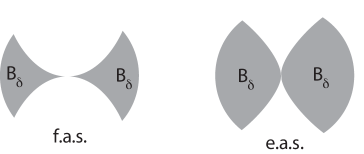
Figure 1: Shape of the basins of attraction ${\cal B}_{\delta}(X)$ for the stability types of Definitions 2.2 (left) and 2.3 (right). The grey region represents the intersection of a basin with a cross-section to $X$.

Definition 2.1.

A compact invariant set $X$ is completely unstable (c.u.) if there exists $\delta>0$ such that $\ell({\cal B}_{\delta}(X))=0$.

Definition 2.2.

A set $X$ is fragmentarily asymptotically stable (f.a.s.) if $\ell({\cal B}_{\delta}(X))>0$ for any $\delta>0$ (see Figure 1).

Definition 2.3.

A set $X$ is essentially asymptotically stable (e.a.s) if

$$\lim_{\delta\to 0}\left(\lim_{\varepsilon\to 0}\frac{\ell(N_{\varepsilon}(X)\setminus{\cal B}_{\delta}(X))}{\ell\left(N_{\varepsilon}(X)\right)}\right)=0,$$

where $N_{\varepsilon}(X)$ denotes $\varepsilon$-neighbourhood of $X$ (see Figure 1).

Definition 2.4.

A set $X$ is asymptotically stable (a.s) if for any $\delta>0$ there exists $\varepsilon>0$ such that $N_{\varepsilon}(X)\subset{\cal B}_{\delta}(X)$.

Note that a.s. implies e.a.s., and e.a.s. implies f.a.s. but the converse does not hold: if a set is a.s. it attracts a full neighbourhood of points; if a set is e.a.s. it attracts a subset of (asymptotically) full measure in its neighbourhood; if a set is f.a.s., it attracts a positive measure set from its any neighbourhood. From the point of view of simulations and applications, sets that are either a.s. or e.a.s. are the ones more likely to be observed.

For a compact invariant set $X\subset{\mathbb{R}}^{n}$, a point $x\in X$, $\delta>0$ and $N_{\varepsilon}(x)$ the ball of centre $x$ and radius $\varepsilon>0$, let

$$S_{\varepsilon,\delta}(x)=\frac{\ell\left({\cal B}_{\delta}(X)\cap N_{\varepsilon}(x)\right)}{\ell\left(N_{\varepsilon}(x)\right)}.$$

Definition 2.5 ([18]).

Let $X$ be a compact invariant set with $x\in X$. Define:

$$\sigma_{loc,-}(x)=\lim_{\delta\to 0}\lim_{\varepsilon\to 0}\frac{\ln S_{\varepsilon,\delta}(x)}{\ln\varepsilon}\quad\mbox{and}\quad\sigma_{loc,+}(x)=\lim_{\delta\to 0}\lim_{\varepsilon\to 0}\frac{\ln\left(1-S_{\varepsilon,\delta}(x)\right)}{\ln\varepsilon}$$

with the conventions that $\sigma_{loc,-}(x)=\infty$ if there is an $\varepsilon_{0}$ such that $S_{\varepsilon,\delta}(x)=0$ for all $\varepsilon<\varepsilon_{0}$, and that $\sigma_{loc,+}(x)=\infty$ if there is an $\varepsilon_{0}$ such that $S_{\varepsilon,\delta}(x)=1$ for all $\varepsilon<\varepsilon_{0}$.

The (local) stability index of $X$ at $x$ is then

$$\sigma(x,X)=\sigma_{loc,+}(x)-\sigma_{loc,-}(x).$$

Note that $\sigma_{loc,\pm}\geq 0$, hence $\sigma(x,X)\in[-\infty,\infty]$.

The stability index $\sigma(x,X)$ is constant for $x$ in a trajectory [18, Theorem 2.2]. If $X$ is either a heteroclinic cycle or a compact heteroclinic network having a connection $\kappa_{ij}$, then this allows us to define $\sigma(\kappa_{ij},X)$ as $\sigma(x,X)$, for some $x\in\kappa_{ij}$.

3 Stability results

We divide our stability results into two types: those that study the network as a whole and those that study stability of fixed points of maps. The main result concerning stability of a network is of a negative kind. We show that many heteroclinic networks never are asymptotically stable. The results pertaining to fixed points of maps may be applicable to other cycles or networks beyond the present case study.

3.1 Stability of networks

In this short subsection, we prove generic results that apply to robust heteroclinic networks in an Euclidean space of any finite dimension. We provide sufficient conditions that prevent a heteroclinic network in ${\mathbb{R}}^{n}$ from being a.s. In particular, we immediately conclude that the network in the case study of this article is not a.s.

Theorem 3.1.

Let $X\subset{\mathbb{R}}^{n}$ be a robust heteroclinic cycle or network with equilibria $\xi_{j}$. Assume that $X$ is compact. If there exists $\xi_{j}\in X$ such that $W^{u}(\xi_{j})\not\subset X$ then $X$ is not asymptotically stable.

Proof.

Since $X$ is compact and $W^{u}(\xi_{j})\not\subset X$, there exist $y\in W^{u}(\xi_{j})$ and $\delta>0$ such that $d(y,X)>\delta$. Denote by $\Phi_{t}(y)$ the trajectory through $y$. Since $\lim_{t\to-\infty}\Phi_{t}(y)=\xi_{j}$, for any $\varepsilon>0$ there exists $T_{\varepsilon}>0$ such that $y_{\varepsilon}=\Phi_{-T_{\varepsilon}}(y)$ satisfies $d(\xi_{j},y_{\varepsilon})<\varepsilon$. Hence, for any $\varepsilon>0$ we have $d(y_{\varepsilon},X)<\varepsilon$ and $d(\Phi_{T_{\varepsilon}}(y_{\varepsilon}),Y)>\delta$. ∎

Corollary 3.2.

Let $X\subset{\mathbb{R}}^{n}$ be a compact robust heteroclinic network comprised of equilibria $\xi_{j}$ and a finite number of one-dimensional connections. Suppose that there exists $\xi_{j}\in X$ such that $\dim W^{u}(\xi_{j})\geq 2$. Then $X$ is not asymptotically stable.

Proof.

Since $X$ is comprised of a finite number of one-dimensional connections, we have $\dim X=1$. Hence, $W^{u}(\xi_{j})\not\subset X$. ∎

Corollary 3.3.

Let $X\subset{\mathbb{R}}^{n}$ be a compact robust heteroclinic network with equilibria $\xi_{j}$. If for some equilibrium $\xi_{j}$ there is a transverse eigenvalue with positive real part then $X$ is not asymptotically stable.

An example of asymptotically stable heteroclinic network with a continuum of one-dimensional connections can be found in [10]. Apparently Corollary 3.2 holds true if a countable number of connections is assumed, but the current statement assuming a finite number of connections is sufficient for our purposes. We remark that an extension of the above results to networks whose nodes are periodic orbits should be possible. However, networks with more complex nodes need extra care. These are outside the scope of this article.

Concerning weaker notions of stability, it follows from the definition of f.a.s. that if $X$ is a robust heteroclinic network such that at least one of its cycles is f.a.s. then $X$ is f.a.s. Examples in [4] show that the same does not hold for e.a.s.

3.2 Stability of fixed points

The following are technical results useful for the study in Section 4. We provide conditions for different types of stability of fixed points of maps. These maps take several forms which are common in return maps to cross-sections to connections of heteroclinic cycles or networks.

Lemma 3.4.

Consider the map ${\bf h}(p,q)=(p^{\gamma\alpha}q^{\gamma\beta},p^{\alpha}q^{\beta})$, ${\bf h}:~{}{\mathbb{R}}_{+}^{2}\to{\mathbb{R}}_{+}^{2}$. The fixed point $(p,q)=(0,0)$ of the map ${\bf h}$ is

• f.a.s. if and only if

  $$\gamma\alpha+\beta>1\hbox{ and }\gamma>0;$$ (1)

• e.a.s. if and only if (1) and $|\max\{\alpha,\beta\}|>|\min\{\alpha,\beta\}|$;

• a.s. if and only if (1), $\alpha>0$ and $\beta>0$.

Proof.

(i) For $n\geq 1$ the iterates $(p_{n},q_{n})={\bf h}^{n}(p_{0},q_{0})$ satisfy $p_{n}=q_{n}^{\gamma}$ and $q_{n+1}=q_{n}^{\gamma\alpha+\beta}$, therefore conditions (1) are necessary. To show that the conditions are sufficient, we note that (1) implies that at least one of $\alpha$ and $\beta$ is positive. Denote $Q_{\delta}=(0,\delta)^{2}$. The points $(p_{0},q_{0})\in Q_{\delta}$ such that

$$p_{0}^{\gamma_{0}\alpha}q_{0}^{\gamma_{0}\beta}<\delta,$$ (2)

where $\gamma_{0}=\min\{1,\gamma\}$, satisfy $(p_{n},q_{n})\in Q_{\delta}$ for any $n\geq 0$. Since (2) is equivalent to

$$p_{0}^{\alpha}q_{0}^{\beta}<\delta^{1/\gamma_{0}},$$

and at least one of $\alpha$ and $\beta$ is positive, the set of such points has positive measure for any $\delta>0$.

(ii, iii) Since e.a.s. and a.s. imply f.a.s., we assume that the conditions (1) are satisfied. As we noted above, at least one of $\alpha$ and $\beta$ is positive. Let $\alpha>0$. From (2), if $\beta$ is positive then all $(p_{0},q_{0})\in Q_{\varepsilon}$, where $0<\varepsilon<\delta^{1/\gamma_{0}(\alpha+\beta)}$, satisfy $(p_{n},q_{n})\in Q_{\delta}$ for any $n\geq 0$, which implies that the origin is a.s. and e.a.s.

For negative $\beta$ we decompose $Q_{\delta}=Q_{\delta}^{I}\cup Q_{\delta}^{II}$, where

$$Q_{\delta}^{I}=\{(p,q)\in Q_{\delta}~{}:~{}p^{\gamma_{0}\alpha}q^{\gamma_{0}\beta}<\delta\},\ Q_{\delta}^{II}=\{(p,q)\in Q_{\delta}~{}:~{}p^{\gamma_{0}\alpha}q^{\gamma_{0}\beta}>\delta\}.$$

By construction, ${\bf h}^{n}(p_{0},q_{0})\in Q_{\delta}$ for any $n\geq 0$ and $(p_{0},q_{0})\in Q_{\delta}^{I}$, while ${\bf h}(p_{0},q_{0})\not\in Q_{\delta}$ for any $(p_{0},q_{0})\in Q_{\delta}^{II}$. Since for any $\varepsilon>0$ the set $Q_{\varepsilon}\cap Q_{\delta}^{II}$ is not empty, the origin is not a.s.

If $\alpha>-\beta$, then

$$\lim_{\varepsilon\to 0}\frac{\ell(Q_{\delta}^{II}\cap Q_{\varepsilon})}{\ell\left(Q_{\varepsilon}\right)}=\lim_{\varepsilon\to 0}\frac{-\beta\delta^{-1/\gamma_{0}\beta}}{\alpha-\beta}\varepsilon^{-\alpha/\beta-1}=0,$$

while for $\alpha<-\beta$

$$\lim_{\varepsilon\to 0}\frac{\ell(Q_{\delta}^{I}\cap Q_{\varepsilon})}{\ell\left(Q_{\varepsilon}\right)}=\lim_{\varepsilon\to 0}\frac{-\alpha\delta^{-1/\gamma_{0}\alpha}}{\alpha-\beta}\varepsilon^{-\beta/\alpha-1}=0.$$

Therefore, for positive $\alpha$ the condition for e.a.s. is that $\alpha>-\beta$. Similarly, for positive $\beta$ the condition for e.a.s. is that $\beta>-\alpha$. Both conditions are satisfied if $|\max\{\alpha,\beta\}|>|\min\{\alpha,\beta\}|$. ∎

Lemma 3.5.

Consider the matrix

$$A=\left(\begin{array}[]{cc}\alpha_{1}&\beta_{1}\\ \alpha_{2}&\beta_{2}\end{array}\right).$$ (3)

If

$$\alpha_{1}\geq 0,\quad\alpha_{2}>0\quad\hbox{ and }\quad\det A<0$$ (4)

then the matrix has real eigenvalues, $\lambda_{+}>0$ and $\lambda_{-}<0$, and $v_{11}v_{12}>0$, where $(v_{11},v_{12})$ is the eigenvector associated with $\lambda_{+}$. Furthermore, $|\lambda_{+}|>|\lambda_{-}|$ if and only if, additionally,

$$\alpha_{1}+\beta_{2}>0.$$ (5)

Proof.

Since $\det A<0$, the matrix has one positive real eigenvalue and one negative, that we denote by $\lambda_{+}$ and $\lambda_{-}$, respectively. Decompose $(1,0)={\bf v}_{1}+{\bf v}_{2}$, where ${\bf v}_{j}=(v_{j1},v_{j2})$, $j=1,2$, $A{\bf v}_{1}=\lambda_{+}{\bf v}_{1}$ and $A{\bf v}_{2}=\lambda_{-}{\bf v}_{2}$. From

$$\left(\begin{array}[]{c}1\\ 0\end{array}\right)={\bf v}_{1}+{\bf v}_{2}\hbox{ and }A\left(\begin{array}[]{c}1\\ 0\end{array}\right)=\lambda_{+}{\bf v}_{1}+\lambda_{-}{\bf v}_{2}$$

we obtain that $v_{11}=(\alpha_{1}-\lambda_{-})/(\lambda_{+}-\lambda_{-})>0$ and $v_{12}=\alpha_{2}/(\lambda_{+}-\lambda_{-})>0$.

Since $\lambda_{+}+\lambda_{-}=\alpha_{1}+\beta_{2}$, the inequality $|\lambda_{+}|>|\lambda_{-}|$ is satisfied if and only if $\alpha_{1}+\beta_{2}$ is positive. ∎

Corollary 3.6.

Suppose the matrix $A$ in (3) satisfies (4) and (5) and let $(x_{1},y_{1})=A(x_{0},y_{0})$, where $x_{1},y_{1},x_{0},y_{0}$ are negative, $y_{1}/x_{1}<y_{0}/x_{0}$. Then the set $V=\{(x,y)\in{\mathbb{R}}^{2}_{-}\ :\ y_{1}/x_{1}\leq y/x\leq y_{0}/x_{0}\}$ is $A$-invariant, i.e. $AV\subset V$.

Proof.

Let $(a,b)$ be the coordinates of points in ${\mathbb{R}}^{2}$ in the basis comprised of eigenvectors of the matrix $A$, ${\bf v}^{+}$ and ${\bf v}^{-}$. Denote by $(a_{0},b_{0})$ and $(a_{1},b_{1})$ the coordinates of $(x_{0},y_{0})$ and $(x_{1},y_{1})$, respectively, and choose the directions of the eigenvectors such that $a_{0}>0$ and $b_{0}>0$. In the coordinates $(a,b)$ the set $V$ is

$$V=\{(a,b)\in{\mathbb{R}}^{2}~{}~{}:~{}~{}a>0,~{}~{}b_{1}/a_{1}\leq b/a\leq b_{0}/a_{0}~{}~{}\}.$$

Since $\lambda_{+}^{2}/\lambda_{-}^{2}>1$ and $A(a,b)=(\lambda_{+}a,\lambda_{-}b)$, for any $(a,b)\in V$ we have

$$b_{1}/a_{1}=\lambda_{-}b_{0}/\lambda_{+}a_{0}\leq\lambda_{-}b/\lambda_{+}a\leq\lambda_{-}b_{1}/\lambda_{+}a_{1}=\lambda_{-}^{2}b_{0}/\lambda_{+}^{2}a_{0}<b_{0}/a_{0},$$

which implies that $V$ is $A$-invariant. ∎

Lemma 3.7.

Consider the map ${\bf h}:~{}{\mathbb{R}}_{+}^{2}\to{\mathbb{R}}_{+}^{2}$,

$${\bf h}(p,q)=(p^{\alpha_{1}}q^{\beta_{1}},p^{\alpha_{2}}q^{\beta_{2}})\hbox{, where }\alpha_{2}>0.$$ (6)

The fixed point $(p,q)=(0,0)$ of the map ${\bf h}$ is

• f.a.s. if and only if all the following conditions hold:

  1. $\alpha_{1}+\beta_{2}>0$,

  2. either $\alpha_{1}+\beta_{2}+\beta_{1}\alpha_{2}-\alpha_{1}\beta_{2}>1$ or $\alpha_{1}+\beta_{2}>2$,

  3. either $\beta_{1}>0$ or $\alpha_{1}-\beta_{2}>0$;

  4. $\left(\alpha_{1}-\beta_{2}\right)^{2}+4\beta_{1}\alpha_{2}\geq 0$;

• a.s. if and only if both conditions below hold:

  1. $\alpha_{1}>0,\beta_{1}>0,\beta_{2}>0$,

  2. either $\alpha_{1}+\beta_{2}+\beta_{1}\alpha_{2}-\alpha_{1}\beta_{2}>1$ or $\alpha_{1}+\beta_{2}>2$.

Moreover, in case (i), if either $\beta_{1}>0$ or $\alpha_{1}+\beta_{2}+\beta_{1}\alpha_{2}-\alpha_{1}\beta_{2}>1$ then condition 4. is redundant.

Proof.

Consider the transition matrix $A$ given in (3) and let $\lambda_{\max}$ be its eigenvalue maximal in absolute value, with associated eigenvector ${\bf v}^{\max}=(v_{1}^{\max},v_{2}^{\max})$. As proved in [16], the fixed point is f.a.s. if and only if

$$\lambda_{\max}\hbox{ is real, }\lambda_{\max}>1\hbox{ and }v_{1}^{\max}v_{2}^{\max}>0.$$

The eigenvalues of $A$ are

$$\lambda_{\pm}=\frac{\alpha_{1}+\beta_{2}}{2}\pm\left(\frac{(\alpha_{1}-\beta_{2})^{2}}{4}+\beta_{1}\alpha_{2}\right)^{1/2},$$ (7)

with the associated eigenvectors

$${\bf v}^{\pm}=\left(\frac{\lambda_{\pm}-\beta_{2}}{\alpha_{2}},1\right).$$ (8)

From (7), the eigenvalues are real if and only if $(\alpha_{1}-\beta_{2})^{2}+4\beta_{1}\alpha_{2}\geq 0$. We have $|\lambda_{+}|>|\lambda_{-}|$ if and only if $\alpha_{1}+\beta_{2}>0$. The inequality $\lambda_{+}>1$ is satisfied if and only if either $\alpha_{1}+\beta_{2}+\beta_{1}\alpha_{2}-\alpha_{1}\beta_{2}>1$ or $\alpha_{1}+\beta_{2}>2$. Finally, (8) implies that $v_{1}^{\max}v_{2}^{\max}=v_{1}^{+}v_{2}^{+}=(\lambda_{+}-\beta_{2})/\alpha_{2}>0$ if and only if either $\beta_{1}\alpha_{2}>0$ or $\alpha_{1}-\beta_{2}>0$.

Because $\alpha_{2}>0$ it follows that $\beta_{1}>0$ is equivalent to $\beta_{1}\alpha_{2}>0$ and this implies that $(\alpha_{1}-\beta_{2})^{2}+4\beta_{1}\alpha_{2}>0$ when the first part of 3. holds. When $\alpha_{1}+\beta_{2}+\beta_{1}\alpha_{2}-\alpha_{1}\beta_{2}>1$ we can write

$$\left(\alpha_{1}-\beta_{2}\right)^{2}+4\beta_{1}\alpha_{2} = \left(\alpha_{1}+\beta_{2}\right)^{2}-4\left(\alpha_{1}\beta_{2}-\beta_{1}\alpha_{2}\right)>$$

$$> \left(\alpha_{1}+\beta_{2}\right)^{2}+4\left(1-(\alpha_{1}+\beta_{2})\right)=\left(\alpha_{1}+\beta_{2}-2\right)^{2}>0$$

Recall [16] that the fixed point $(0,0)$ of the map (6) is a.s. if and only if all entries of the matrix $A$ are non-negative and $\lambda_{\max}>1$. Condition 1. of part (ii) is equivalent to the non-negativity of the entries of $A$. Due to (7), $\alpha_{1}+\beta_{2}>0$ implies $\lambda_{\max}=\lambda_{+}$, and from the arguments above, part (ii) is proven. ∎

The next two lemmas provide conditions for the stability of the fixed point of a map of the form ${\bf h}(p,q)=(\max\{p^{\gamma\alpha_{2}}q^{\gamma\beta_{2}},p^{\alpha_{1}}q^{\beta_{1}}\},p^{\alpha_{2}}q^{\beta_{2}})$, depending on relations among parameters. These lemmas are used to study the stability of cycles ${\cal C}_{123}$ and ${\cal C}_{143}$ in Section 4, for which the signs are as given in the statement of the lemmas. So, we prove the lemmas in the restricted form that is sufficient for our purposes, although similar proofs may be given for other parameter ranges.

Lemma 3.8.

Consider the map ${\bf h}:~{}{\mathbb{R}}_{+}^{2}\to{\mathbb{R}}_{+}^{2}$,

$${\bf h}(p,q)=(\max\{p^{\gamma\alpha_{2}}q^{\gamma\beta_{2}},p^{\alpha_{1}}q^{\beta_{1}}\},p^{\alpha_{2}}q^{\beta_{2}})\hbox{, where }$$

$$\alpha_{1}\geq 0,\ \alpha_{2}>0,\ \gamma\alpha_{2}-\alpha_{1}>0\hbox{ and }\gamma_{1}=\frac{\beta_{1}-\gamma\beta_{2}}{\gamma\alpha_{2}-\alpha_{1}}>\gamma.$$

The fixed point $(p,q)=(0,0)$ of the map ${\bf h}$ is

• not f.a.s. if either $\gamma<0$ or $\gamma\alpha_{2}+\beta_{2}<1;$

• not e.a.s. if $\alpha_{2}<-\beta_{2};$

• not a.s. if $\beta_{2}<0$.

• f.a.s. if $\gamma>0$ and $\gamma\alpha_{2}+\beta_{2}>1;$

• e.a.s. if $\gamma>0$, $\gamma\alpha_{2}+\beta_{2}>1$ and $\alpha_{2}>-\beta_{2};$

• a.s. if $\gamma>0$, $\gamma\alpha_{2}+\beta_{2}>1$ and $\beta_{2}>0.$

Proof.

Evidently, $\gamma\leq 0$ implies that the map is completely unstable, hence till the end of the proof we assume that $\gamma>0$. The result is local, therefore we work on $V_{\varepsilon}=\{(p,q)\in{\mathbb{R}}^{2}~{}:~{}0<p<\varepsilon,~{}0<q<\varepsilon\}$, with $0<\varepsilon<1$, that we decompose as $V_{\varepsilon}=U^{I}\cup U^{II}$ where

$$U^{I}=\{(p,q)\in V_{\varepsilon}~{}:~{}~{}{\bf h}(p,q)={\bf h}^{I}(p,q)\equiv(p^{\gamma\alpha_{2}}q^{\gamma\beta_{2}},p^{\alpha_{2}}q^{\beta_{2}})\},$$ (9)

$$U^{II}=\{(p,q)\in V_{\varepsilon}~{}:~{}~{}{\bf h}(p,q)={\bf h}^{II}(p,q)\equiv(p^{\alpha_{1}}q^{\beta_{1}},p^{\alpha_{2}}q^{\beta_{2}})\}.$$ (10)

These sets, shown in Figure 2 can also be written as

$$U^{I}=\{(p,q)\in V_{\varepsilon}~{}:~{}~{}p\geq q^{\gamma_{1}}\}\qquad\mbox{and}\qquad U^{II}=\{(p,q)\in V_{\varepsilon}~{}:~{}~{}p\leq q^{\gamma_{1}}\}.$$

Recall, from the proof of Lemma 3.4, that ${\bf h}^{I}(p,q)=(p_{1},q_{1})=(q^{\gamma}_{1},q_{1})$. Hence, for any $(p,q)\in U^{I}$, we have ${\bf h}(p,q)=(p_{1},q_{1})$ where $p_{1}=q^{\gamma}_{1}>q^{\gamma_{1}}_{1}$. Therefore, ${\bf h}(U^{I})$ is contained in the curve $p=q^{\gamma}$ and in particular ${\bf h}(U^{I})\subset U^{I}$ (see Figure 2).

For $(p,q)\in U^{II}$, again let ${\bf h}(p,q)=(p_{1},q_{1})={\bf h}^{II}(p,q)$. We have that $q_{1}=p^{\alpha_{2}}q^{\beta_{2}}$ and, by definition of $U^{II}$, that $p_{1}=p^{\alpha_{1}}q^{\beta_{1}}>p^{\gamma\alpha_{2}}q^{\gamma\beta_{2}}=q_{1}^{\gamma}>q_{1}^{\gamma_{1}}$. Hence, ${\bf h}(p,q)=(p_{1},q_{1})\in U^{I}$.

Thus, the conditions for stability are those given in Lemma 3.4 for the map ${\bf h}^{I}$. ∎

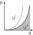
Figure 2: Under the conditions of Lemma 3.8 with $\gamma>0$ the white set $U^{I}$ with boundary in the solid line $p=q^{\gamma_{1}}$ is mapped by ${\bf h}$ into the dashed curve $p=q^{\gamma}$, that is contained in $U^{I}$. The grey set $U^{II}$ is mapped inside $U^{I}$.Here we show the case $\gamma>1$.

Lemma 3.9.

Consider the map ${\bf h}:~{}{\mathbb{R}}_{+}^{2}\to{\mathbb{R}}_{+}^{2}$,

$${\bf h}(p,q)=(\max\{p^{\gamma\alpha_{2}}q^{\gamma\beta_{2}},p^{\alpha_{1}}q^{\beta_{1}}\},p^{\alpha_{2}}q^{\beta_{2}})\hbox{, where }$$

$$\alpha_{1}\geq 0,\ \alpha_{2}>0,\ \ \beta_{1}\alpha_{2}-\alpha_{1}\beta_{2}>0,\gamma\alpha_{2}-\alpha_{1}>0\hbox{ and }\gamma_{1}=\frac{\beta_{1}-\gamma\beta_{2}}{\gamma\alpha_{2}-\alpha_{1}}<\gamma.$$

• Assume in addition that $\alpha_{1}+\beta_{2}>0$. The fixed point $(p,q)=(0,0)$ of the map ${\bf h}$ is:

  • not f.a.s. if either $\gamma<0$ or $\alpha_{1}+\beta_{2}+\beta_{1}\alpha_{2}-\alpha_{1}\beta_{2}<1$;

  • not a.s. if either $\beta_{1}<0$ or $\beta_{2}<0$;

  • f.a.s. if $\gamma>0$ and $\alpha_{1}+\beta_{2}+\beta_{1}\alpha_{2}-\alpha_{1}\beta_{2}>1$;

  • a.s. if $\beta_{1}>0$, $\beta_{2}>0$, $\gamma>0$ and $\alpha_{1}+\beta_{2}+\beta_{1}\alpha_{2}-\alpha_{1}\beta_{2}>1$.

• Assume in addition that $\alpha_{1}+\beta_{2}<0$. The fixed point $(p,q)=(0,0)$ of the map ${\bf h}$ is:

  • not f.a.s. if either $\gamma<0$ or $\alpha_{2}(\gamma\alpha_{1}+\beta_{1})+\beta_{2}(\gamma\alpha_{2}+\beta_{2})<1$;

  • f.a.s. if $\gamma>0$ and $\alpha_{2}(\gamma\alpha_{1}+\beta_{1})+\beta_{2}(\gamma\alpha_{2}+\beta_{2})>1$;

  • never a.s.

The conditions may be interpreted in terms of the matrix $A$ of (3) and its eigenvalues, as follows: $\alpha_{1}+\beta_{2}$ is the trace of the matrix $A$, hence it has the same sign as $|\lambda_{+}|-|\lambda_{-}|$. Thus $\alpha_{1}+\beta_{2}>0$ means that the eigenvalues of $A$ satisfy $|\lambda_{+}|>|\lambda_{-}|$. If $p(\lambda)$ is the characteristic polynomial of $A$, then $p(1)<0$ implies that $\lambda_{+}>1$ and $p(1)=-(\alpha_{1}+\beta_{2}+\beta_{1}\alpha_{2}-\alpha_{1}\beta_{2})+1$. The condition $\beta_{1}\alpha_{2}-\alpha_{1}\beta_{2}>0$ means $\det A<0$.

             

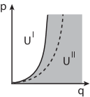
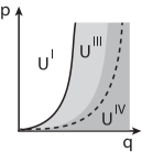
Figure 3: Under the conditions of Lemma 3.9 with $\gamma>0$ the white set $U^{I}$ with boundary in the solid line $p=q^{\gamma_{1}}$ is mapped by ${\bf h}$ into the dashed curve $p=q^{\gamma}$, that is contained in the grey set $U^{II}$. The latter set can be further subdivided in two components that, in case (a) when $\alpha_{1}+\beta_{2}>0$, are mapped as ${\bf h}(U^{IV})\subset U^{I}$, ${\bf h}(U^{I})\subset U^{III}$ and ${\bf h}(U^{III})\subset U^{III}$, shown in the middle. Further iterates of points in $U^{III}$ approach a line in $U^{III}$. Case(b) is shown on the right, where ${\bf h}(U^{IV})\subset U^{I}$, ${\bf h}(U^{I})\subset U^{IV}$ and for $(p,q)\in U^{III}$ the iterates ${\bf h}^{n}(p,q)$ either escape from $V_{\varepsilon}$ or ${\bf h}^{n}(p,q)\in U^{IV}$ for some $0<n<\infty$.

Proof.

As in the proof of Lemma 3.8, we decompose $V_{\varepsilon}=U^{I}\cup U^{II}$, where the sets $U^{I}$ and $U^{II}$ are defined in (9) and (10). Again, ${\bf h}$ maps $U^{I}$ into the curve $p=q^{\gamma}$, but now this curve is contained in $U^{II}$ (see Figure 3). Let $\gamma_{0}=(\beta_{1}-\gamma_{1}\beta_{2})/(\gamma_{1}\alpha_{2}-\alpha_{1})$, if $\gamma_{0}>0$ then decompose further $U^{II}=U^{III}\cup U^{IV}$, where

$$U^{III}=\{(p,q)\in U^{II}:~{}{\bf h}(p,q)\in U^{II}\}=\{(p,q)\in U^{II}:~{}q^{\gamma_{0}}\leq p\leq q^{\gamma_{1}}\}$$

and

$$U^{IV}=\{(p,q)\in U^{II}:~{}{\bf h}(p,q)\in U^{I}\}=\{(p,q)\in U^{II}:~{}p\leq q^{\gamma_{0}}\}.$$

If $\gamma_{0}\leq 0$ then the set $U^{IV}$ is empty and $U^{III}$ coincides with $U^{II}$.

Let $W_{\varepsilon}=\{(x,y)\in{\mathbb{R}}^{2}_{-}:~{}x<\ln\varepsilon,~{}y<\ln\varepsilon\}$. In the variables $(x,y)=(\ln p,\ln q)$ the sets $U^{I}$, $U^{III}$ and $U^{IV}$ are (see Figure 3):

$$\begin{array}[]{l}U^{I}=\{(x,y)\in W_{\varepsilon}:~{}x\geq\gamma_{1}y\},\\ U^{III}=\{(x,y)\in W_{\varepsilon}:~{}\gamma_{0}y\leq x\leq\gamma_{1}y\},\\ U^{IV}=\{(x,y)\in W_{\varepsilon}:~{}x\leq\gamma_{0}y\}.\end{array}$$

Let $(x_{0},y_{0})=-(\gamma_{0},1)$, $(x_{1},y_{1})=A(x_{0},y_{0})$ and $(x_{2},y_{2})=A^{2}(x_{0},y_{0})$. Our choice of $\gamma_{0}$ and $\gamma_{1}$ implies that $x_{1}/y_{1}=\gamma_{1}$ and $x_{2}/y_{2}=\gamma$. In the variables $(a,b)$ employed in the proof of Corollary 3.6 the sets $U^{I}$, $U^{III}$ and $U^{IV}$ satisfy:

$$\begin{array}[]{l}U^{III}\subset\{~{}(a,b)\in{\mathbb{R}}^{2}~{}:~{}a>0,~{}b_{1}/a_{1}\leq b/a\leq b_{0}/a_{0}~{}\}\\ U^{I}\subset\{~{}(a,b)\in{\mathbb{R}}^{2}~{}:~{}b/a\leq b_{1}/a_{1}~{}\}\\ U^{IV}\subset\{~{}(a,b)\in{\mathbb{R}}^{2}~{}:~{}b/a\geq b_{0}/a_{0}~{}\}.\end{array}$$

As stated, the conditions for stability depend on the sign of $\alpha_{1}+\beta_{2}$. Below we consider the cases of positive and negative $\alpha_{1}+\beta_{2}$ separately. (Note, that generically the sum does not vanish.)

(a) Assume that $\alpha_{1}+\beta_{2}>0$. Corollary 3.6 implies that the set $U^{III}$ is ${\bf h}$-invariant. In particular, $(\gamma y^{\prime},y^{\prime})=A(\gamma_{1}y,y)\subset U^{III}$. For $(a^{\prime},b^{\prime})=A(a,b)$, where $(a,b)\in U^{IV}$ and $a>0$, we have $b^{\prime}/a^{\prime}=\lambda_{-}b/\lambda_{+}a<\lambda_{-}b_{0}/\lambda_{+}a_{0}=b_{1}/a_{1}$. Therefore,

$$\left({\bf h}\left(U^{IV}\right)\cap W_{\varepsilon}\right)\subset U^{I}.$$

If $(x,y)\in U^{I}$ then $(x^{\prime},y^{\prime})={\bf h}(x,y)$ satisfies $x^{\prime}=\gamma y^{\prime}$. Therefore, $\left({\bf h}\left(U^{I}\right)\cap W_{\varepsilon}\right)\subset U^{III}$ (see Figure 3). In the original variables $(p,q)$ the inclusions can be summarised as

$${\bf h}\left(U^{III}\right)\subset U^{III},\quad\left({\bf h}\left(U^{I}\right)\cap V_{\varepsilon}\right)\subset U^{III},\quad\left({\bf h}\left(U^{IV}\right)\cap V_{\varepsilon}\right)\subset U^{I}.$$

Hence,

$$\left({\bf h}\left({\bf h}\left(V_{\varepsilon}\right)\cap V_{\varepsilon}\right)\cap V_{\varepsilon}\right)\subset U^{III}$$

and for any $(p,q)\in V_{\varepsilon}$ and $n\geq 2$ we have that either ${\bf h}^{n}(p,q)\in U^{III}$ or ${\bf h}^{n}(p,q)\notin V_{\varepsilon}$. Therefore, the conditions for stability are those given in Lemma 3.7 for the map ${\bf h}^{II}$.

(b) Assume that $\alpha_{1}+\beta_{2}<0$. Therefore, $\beta_{2}<0$ and the map is not a.s. To find conditions for f.a.s., note that in the coordinates $(a,b)$ the iterates $(a_{n},b_{n})=A^{n}(a_{0},b_{0})$ satisfy $b_{n}/a_{n}=\lambda_{-}^{n}b_{0}/\lambda_{+}^{n}a_{0}$. Since $|\lambda_{-}|>|\lambda_{+}|$, for any $(a,b)\in U^{III}$ with $b\neq 0$ the iterates ${\bf h}^{n}(a,b)$ escape from $U^{III}$ for some finite $n>0$. Moreover, we have $\left({\bf h}\left(U^{IV}\right)\cap W_{\varepsilon}\right)\subset U^{I}$ (by the same arguments as in the case $\alpha_{1}+\beta_{2}>0$) and $\left({\bf h}\left(U^{I}\right)\cap W_{\varepsilon}\right)\subset U^{VI}$ (since $(\gamma y^{\prime},y^{\prime})=A(\gamma_{1}y,y)\subset U^{IV}$). Returning to the original coordinates $(p,q)$ (see Figure 3) we proved that

$$\begin{array}[]{l}{\bf h}^{n_{0}}(p,q)\cap V_{\varepsilon}\in U^{IV}\hbox{for some $n_{0}>0$, for almost all }(p,q)\in U^{III},\\ \left({\bf h}\left(U^{IV}\right)\cap V_{\varepsilon}\right)\subset U^{I},\qquad\left({\bf h}\left(U^{I}\right)\cap V_{\varepsilon}\right)\subset U^{IV}.\end{array}$$

Hence, for almost all initial conditions there exists $n>0$ such that the iterates $(p_{n},q_{n})={\bf h}^{n}(p,q)$ satisfy either $(p_{n},q_{n})\not\in V_{\varepsilon}$ or $(p_{n},q_{n})\in U^{IV}$. In the latter case $(p_{n},q_{n})=(s^{\gamma},s)$. Further iterates satisfy

$$(p_{n+2},q_{n+2})={\bf h}^{n+2}(p_{n},q_{n})={\bf h}^{2}(s^{\gamma},s)={\bf h}^{I}({\bf h}^{II}(s^{\gamma},s))=$$

$${\bf h}^{I}(s^{\alpha_{1}\gamma+\beta_{1}},s^{\alpha_{2}\gamma+\beta_{2}})=(s^{\gamma\alpha_{2}(\alpha_{1}\gamma+\beta_{1})+\gamma\beta_{2}(\alpha_{2}\gamma+\beta_{2})},s^{\alpha_{2}(\alpha_{1}\gamma+\beta_{1})+\beta_{2}(\alpha_{2}\gamma+\beta_{2})}),$$

which implies that the map is f.a.s. whenever $\alpha_{2}(\alpha_{1}\gamma+\beta_{1})+\beta_{2}(\alpha_{2}\gamma+\beta_{2})>1$. ∎

4 Case study: a heteroclinic network from a convection problem

We study a heteroclinic network supported by the following vector field, given as equations (21) in [3]:

$$\left\{\begin{array}[]{l}\dot{x}_{1}=x_{1}[\lambda_{1}+A_{1}x_{1}^{2}+A_{2}(x_{2}^{2}+x_{3}^{2})+C_{1}y_{1}^{2}+C_{2}(y_{2}^{2}+y_{3}^{2})]+A_{3}x_{1}x_{2}^{2}x_{3}^{2}+C_{3}x_{1}y_{2}y_{3}\\ \dot{x}_{2}=x_{2}[\lambda_{1}+A_{1}x_{2}^{2}+A_{2}(x_{1}^{2}+x_{3}^{2})+C_{1}y_{2}^{2}+C_{2}(y_{1}^{2}+y_{3}^{2})]+A_{3}x_{1}^{2}x_{2}x_{3}^{2}+C_{3}x_{2}y_{1}y_{3}\\ \dot{x}_{3}=x_{3}[\lambda_{1}+A_{1}x_{3}^{2}+A_{2}(x_{1}^{2}+x_{2}^{2})+C_{1}y_{3}^{2}+C_{2}(y_{1}^{2}+y_{2}^{2})]+A_{3}x_{1}^{2}x_{2}^{2}x_{3}+C_{3}x_{3}y_{1}y_{2}\\ \dot{y}_{1}=y_{1}[\lambda_{2}+B_{1}y_{1}^{2}+B_{2}(y_{2}^{2}+y_{3}^{2})+C_{4}x_{1}^{2}+C_{5}(x_{2}^{2}+x_{3}^{2})]+B_{3}y_{1}y_{2}^{2}y_{3}^{2}+C_{6}(y_{2}x_{3}^{2}+y_{3}x_{2}^{2})\\ \dot{y}_{2}=y_{2}[\lambda_{2}+B_{1}y_{2}^{2}+B_{2}(y_{1}^{2}+y_{3}^{2})+C_{4}x_{2}^{2}+C_{5}(x_{1}^{2}+x_{3}^{2})]+B_{3}y_{1}^{2}y_{2}y_{3}^{2}+C_{6}(y_{3}x_{1}^{2}+y_{1}x_{3}^{2})\\ \dot{y}_{3}=y_{3}[\lambda_{2}+B_{1}y_{3}^{2}+B_{2}(y_{1}^{2}+y_{2}^{2})+C_{4}x_{3}^{2}+C_{5}(x_{1}^{2}+x_{2}^{2})]+B_{3}y_{1}^{2}y_{2}^{2}y_{3}+C_{6}(y_{1}x_{2}^{2}+y_{2}x_{1}^{2}).\end{array}\right.$$ (11)

This vector field is equivariant under the action in ${\mathbb{R}}^{6}$ of the group ${\bf D}_{3}\times{\bf Z}_{2}\times{\bf Z}_{2}$, generated by:

$$\rho.(x_{1},x_{2},x_{3};y_{1},y_{2},y_{3}) = (x_{2},x_{3},x_{1};y_{2},y_{3},y_{1})$$

$$s_{1}.(x_{1},x_{2},x_{3};y_{1},y_{2},y_{3}) = (x_{1},x_{3},x_{2};y_{1},y_{3},y_{2})$$

$$r.(x_{1},x_{2},x_{3};y_{1},y_{2},y_{3}) = -(x_{1},x_{2},x_{3};y_{1},y_{2},y_{3})$$

$$\gamma^{1}_{\pi}.(x_{1},x_{2},x_{3};y_{1},y_{2},y_{3}) = (x_{1},-x_{2},-x_{3};y_{1},y_{2},y_{3})$$

$$\gamma^{2}_{\pi}.(x_{1},x_{2},x_{3};y_{1},y_{2},y_{3}) = (-x_{1},-x_{2},x_{3};y_{1},y_{2},y_{3}).$$

4.1 Description

In this subsection we introduce notation that is used in the paper. The network involves five (isotropy types of) steady states of (11) and is shown in Figure 4. Here we denote equilibria by $\xi_{j}$. The correspondence to the notation in [3] is as follows:

$$\begin{array}[]{lll}R_{z}:&\xi_{1}=&(x,0,0;0,0,0)\\ \rho^{2}PQ_{w}:&\xi_{2}=&(0,0,0;0,y,y)\\ R_{w}:&\xi_{3}=&(0,0,0;y,0,0)\\ \rho^{2}{\widetilde{PQ}}_{w}&\xi_{4}=&(0,0,0;0,y,-y)\\ \rho^{2}PQ_{z}:&\xi_{5}=&(0,x,x;0,0,0)\end{array}$$

and $[\xi_{j}]$ denotes the group orbit of $\xi_{j}$. By $\kappa_{ij}$ we denote a heteroclinic connection from $\xi_{i}$ to $\xi_{j}$.

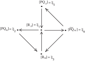
Figure 4: The network of the case study and its cycles.

By ${\cal C}_{123}$, ${\cal C}_{143}$ and ${\cal C}_{145}$ we denote the cycles $[\xi_{1}\to\xi_{2}\to\xi_{3}]$, $[\xi_{1}\to\xi_{4}\to\xi_{3}]$ and $[\xi_{1}\to\xi_{4}\to\xi_{5}]$, respectively. Conditions for the existence of the network are given in Table 4 of [3].

A local basis near $\xi_{j}$ is comprised of ${{\bf e}}_{jk}$, $k=1,\ldots,6$, which are eigenvectors of $df(\xi_{j})$. When $df(\xi_{j})$ has an eigenspace of dimension larger than one, we can use another basis, which is denoted $\tilde{{\bf e}}_{jk}$. For the node $\xi_{3}$ we will also need an extra basis, $\hat{\bf e}_{3k}$, near $\rho\xi_{3}$. The local bases are shown in Table 1 in Appendix B. Local coordinates (i.e. with an origin at $\xi_{j}$) at these bases are denoted by $u_{jk}$, or $\tilde{u}_{jk}$, respectively.The eigenvalue of $df(\xi_{j})$ associated with ${{\bf e}}_{jk}$ is $\lambda_{jk}$.

Tables 2 and 3 of Appendix B provide the isotypic decompositions, while Table 4 has the eigenvalues and eigenvectors at the nodes.

4.2 Stability of the cycles

In this section we derive conditions for stability of individual cycles and the whole network.

4.2.1 The cycle ${\cal C}_{123}=[R_{z}\to PQ_{w}\to R_{w}\to R_{z}]$

In this section we study a cycle that in the quotient space is $[R_{z}\to PQ_{w}\to R_{w}\to R_{z}]$, namely, we derive conditions for the stability of this cycle. Since the cycle is a part of a network, it is not asymptotically stable. As shown in [3], a trajectory near the cycle follows equilibria in a certain order. For definiteness we study asymptotic stability of the cycle

$$R_{w}\to R_{z}\to\rho^{2}PQ_{w}\to\rho R_{w}\qquad\mbox{that is}\qquad\xi_{3}\to\xi_{1}\to\xi_{2}\to\rho\xi_{3}.$$ (12)

Existence of a trajectory that follows such a sequence of equilibria is shown in [3, Section 6] and a numerical simulation appears as [3, Figure 4].

Since the cycle is a part of a network and equilibria are stable in the transverse directions, the eigenvalues $\lambda_{ij}$ of $df(\xi_{i})$, $i=1,2,3$, given in Table 4, satisfy:

$$\begin{array}[]{lcl}\lambda_{1j}<0,\ j=1,2,3,4,&&\lambda_{2j}<0,\ j=1,2,3,4,5,\\ \lambda_{3j}<0,\ j=2,4,5,&&\lambda_{15},\lambda_{16},\lambda_{26},\lambda_{31}>0.\end{array}$$ (13)

We remark that the relative magnitude of $\lambda_{15}$ and $\lambda_{16}$ determines the relative size of the set of points that follow from $\xi_{1}$ to $\xi_{2}$ or to $\xi_{4}$. If $\lambda_{15}>\lambda_{16}$ then more points follow to $\xi_{2}$ along this cycle.

We prove the following theorem:

Theorem 4.1.

Consider the cycle ${\cal C}_{123}$ and assume that the conditions (13) are satisfied. Denote

$$\beta_{1}=\frac{\lambda_{21}\lambda_{35}}{\lambda_{26}\lambda_{31}}(1-\frac{\lambda_{16}}{\lambda_{15}}),\qquad\beta_{2}=-\frac{\lambda_{32}}{\lambda_{31}}+\frac{\lambda_{35}\lambda_{12}}{\lambda_{31}\lambda_{15}}+\frac{\lambda_{35}\lambda_{22}}{\lambda_{31}\lambda_{26}}\left(1-\frac{\lambda_{16}}{\lambda_{15}}\right)$$ (14)

Then

• If

  $$\lambda_{15}<\lambda_{16}\hbox{ or }\beta_{1}+\beta_{2}<1,$$

  then the cycle c.u.

• If

  $$\lambda_{15}>\lambda_{16}\hbox{ and }\beta_{1}+\beta_{2}>1,$$ (15)

  then the cycle is e.a.s. The stability indices are:

  $$\sigma(\kappa_{31},{\cal C}_{123})=1-\lambda_{16}/\lambda_{15},\quad\sigma(\kappa_{23},{\cal C}_{123})=+\infty,\quad\sigma(\kappa_{12},{\cal C}_{123})=+\infty,$$

Proof.

We approximate the behaviour of trajectories near the cycle by a return map, which is a composition of local (approximating behaviour of trajectories near the steady state) and global (approximating behaviour near heteroclinic connections) maps. We start by calculating expressions for these maps, from which we derive the expression for the return map $\tilde{\bf g}:H_{3}^{{\rm in}}\to H_{3}^{{\rm in}}$ where $H_{3}^{{\rm in}}$ is a cross-section of the connection $\rho^{2}PQ_{w}\to\rho R_{w}$ near $\rho R_{w}$. Then we derive conditions for asymptotic stability of the map $\tilde{\bf g}$. Because of its complexity, the proof of stability conditions of the map $\tilde{\bf g}$ is given in Appendix A. Finally, we prove that the cycle is e.a.s. whenever the map $\tilde{\bf g}$ is a.s. and calculate stability indices of the cycle.

The return map is the superposition of local maps $\phi_{j}:\ H^{\rm in}_{j}\to H^{\rm out}_{j}$ and global maps $\psi_{ij}:\ H^{\rm out}_{i}\to H^{\rm in}_{j}$. Here $H_{j}^{\rm in}$ and $H_{j}^{\rm out}$ denote the cross-sections near $\xi_{j}$ to the connections to and from $\xi_{j}$, respectively. Cross-sections are taken to be 4-dimensional, since we can disregard the radial direction at each equilibrium. When we need to specify that the norm of points in the cross-section is smaller than $\varepsilon$ we write $H^{\rm in}_{j}(\varepsilon)$. In each cross-section near $\xi_{j}$, we use coordinates $u_{ji}^{\rm in}$ and $u_{ji}^{\rm out}$ in the direction of the connections from and to $\xi_{i}$, respectively.

A local map near $\xi_{j}\in L_{j}$, where $L_{j}={\rm Fix}\,\Delta_{j}$, depends on the symmetry group $\Delta_{j}$, or to be more precise on the isotypic decomposition of ${\mathbb{R}}^{6}\ominus L_{j}$ under $\Delta_{j}$, and on eigenvalues of $df(\xi_{j})$. The isotypic decomposition of ${\mathbb{R}}^{6}\ominus L_{j}$ is given in Table 2 of Appendix B and local bases near equilibria are given in Table 1 of Appendix B.

The local maps $H^{\rm in}_{j}\to H^{\rm out}_{j}$ are obtained from the flow of the linearised equations, as follows. We compute the flight time from $H^{\rm in}_{j}$ to $H^{\rm out}_{j}$ and then $\phi_{j}$ is obtained substituting this flight time in the other coordinates, to get:

$$\begin{array}[]{cl}\phi_{1}:\ H^{\rm in}_{1}\to H^{\rm out}_{1}&u_{12}^{\rm out}=u_{12}^{\rm in}|u_{15}^{\rm in}|^{-\lambda_{12}/\lambda_{15}},\ u_{13}^{\rm out}=u_{13}^{\rm in}|u_{15}^{\rm in}|^{-\lambda_{13}/\lambda_{15}},\\ &u_{14}^{\rm out}=D_{2}|u_{15}^{\rm in}|^{-\lambda_{14}/\lambda_{15}},\ u_{16}^{\rm out}=u_{16}^{\rm in}|u_{15}^{\rm in}|^{-\lambda_{16}/\lambda_{15}}\\ \phi_{2}:\ H^{\rm in}_{2}\to H^{\rm out}_{2}&u_{21}^{\rm out}=D_{3}|u_{26}^{\rm in}|^{-\lambda_{21}/\lambda_{26}},\ u_{22}^{\rm out}=u_{22}^{\rm in}|u_{26}^{\rm in}|^{-\lambda_{22}/\lambda_{26}},\\ &u_{23}^{\rm out}=u_{23}^{\rm in}|u_{26}^{\rm in}|^{-\lambda_{23}/\lambda_{26}},\ u_{24}^{\rm out}=u_{24}^{\rm in}|u_{26}^{\rm in}|^{-\lambda_{24}/\lambda_{26}},\\ \phi_{3}:\ H^{\rm in}_{3}\to H^{\rm out}_{3}&u_{32}^{\rm out}=u_{32}^{\rm in}|u_{31}^{\rm in}|^{-\lambda_{32}/\lambda_{31}},\ u_{33}^{\rm out}=u_{33}^{\rm in}|u_{31}^{\rm in}|^{-\lambda_{33}/\lambda_{31}},\\ &u_{35}^{\rm out}=u_{35}^{\rm in}|u_{31}^{\rm in}|^{-\lambda_{35}/\lambda_{31}},\ u_{36}^{\rm out}=D_{1}|u_{31}^{\rm in}|^{-\lambda_{36}/\lambda_{31}},\\ \end{array}$$ (16)

where $D_{1}$, $D_{2}$ and $D_{3}$ are positive.

When an equilibrium $\xi_{i}$ belongs to several different cycles, the local map near it depends on the cycle chosen, since the transverse directions are different. However we use the same notation $\phi_{i}$ for the different local maps at $\xi_{i}$ and this should not confuse the reader, since the calculations for each cycle are totally independent and occur in different sections.

A global map along $\kappa_{ij}=[\xi_{i}\to\xi_{j}]$, $\kappa_{ij}\subset P_{ij}$, where $P_{ij}={\rm Fix}\,\Sigma_{ij}$, is predominantly linear. In order to study stability, it is essential to determine which coefficients of the linear map vanish. This, in turn, depends on the isotypic decomposition of ${\mathbb{R}}^{6}\ominus P_{ij}$ under $\Sigma_{ij}$ provided in Appendix B. For the global maps $\psi_{ij}:H^{\rm out}_{i}\to H^{\rm in}_{j}$ we take linear approximations:

$$\begin{array}[]{cl}\psi_{12}:\ H^{\rm out}_{1}\to H^{\rm in}_{2}&u_{22}^{\rm in}=B_{1}u_{12}^{\rm out},\ u_{23}^{\rm in}=B_{2}u_{13}^{\rm out},\ u_{24}^{\rm in}=B_{3}u_{14}^{\rm out},\ u_{26}^{\rm in}=B_{4}u_{16}^{\rm out}\\ \psi_{23}:\ H^{\rm out}_{2}\to H^{\rm in}_{3}&\hat{u}_{31}^{\rm in}=C_{1}u_{22}^{\rm out}+C_{2}u_{23}^{\rm out},\\ &\hat{u}_{32}^{\rm in}=C_{3}u_{21}^{\rm out},\ \hat{u}_{33}^{\rm in}=C_{4}u_{22}^{\rm out}+C_{5}u_{23}^{\rm out},\ \hat{u}_{35}^{\rm in}=C_{6}u_{24}^{\rm out}\\ \psi_{31}:\ H^{\rm out}_{3}\to H^{\rm in}_{1}&u_{12}^{\rm in}=A_{1}\tilde{u}_{32}^{\rm out},\ u_{13}^{\rm in}=A_{2}\tilde{u}_{33}^{\rm out},\ u_{15}^{\rm in}=A_{3}\tilde{u}_{35}^{\rm out},\ u_{16}^{\rm in}=A_{4}\tilde{u}_{36}^{\rm out},\end{array}$$ (17)

where $A_{j}$, $B_{j}$, $C_{3}$ and $C_{6}$ are positive.

Therefore, the return map $\tilde{{\bf g}}:\,H^{\rm in}_{3}\to H^{\rm in}_{3}$ is given by the composition

$$\tilde{{\bf g}}=\psi_{23}\phi_{2}\psi_{12}\phi_{1}\psi_{31}\phi_{3},$$

which also involves the change of coordinates

$$\begin{array}[]{cc}\tilde{u}_{32}^{\rm in}=(u_{32}^{\rm in}+u_{33}^{\rm in})/\sqrt{2},&\tilde{u}_{33}^{\rm in}=(u_{32}^{\rm in}-u_{33}^{\rm in})/\sqrt{2},\\ \tilde{u}_{35}^{\rm in}=(u_{35}^{\rm in}+u_{36}^{\rm in})/\sqrt{2},&\tilde{u}_{36}^{\rm in}=(u_{35}^{\rm in}-u_{36}^{\rm in})/\sqrt{2}.\end{array}$$ (18)

Stability properties of the map $\tilde{\bf g}$ are studied in Appendix A. It is shown that for almost all (except for a set of zero measure) points in a neighbourhood $V_{\varepsilon}\subset{\mathbb{R}}^{4}$ for sufficiently small $\varepsilon$ and large $n$ the asymptotic behaviour of $\tilde{\bf g}^{n}$ can be approximated by a map ${\bf h}:{\mathbb{R}}^{2}_{+}\to{\mathbb{R}}^{2}_{+}$, ${\bf h}(p,q)=(\max\{pq^{\beta_{2}},q^{\beta_{1}}\},pq^{\beta_{2}})$, where $p=\max\{|x_{1}|,|x_{2}|\}$, $q=\max\{|x_{3}|,|x_{4}|\}$ and the $\beta$’s are given by (14). Unfortunately, we cannot directly apply results of Lemmas 3.8 and 3.9, since there are sets where components of $\tilde{\bf g}$ vanish, while the components of ${\bf h}$ are non zero. Similarly to the proof of Lemmas 3.8 and 3.9, we define sets $U^{I}-U^{III}$, which are subsets of $V_{\varepsilon}$, and show that, depending on relations of parameters of the problem, one of these sets is $\tilde{\bf g}$-invariant for sufficiently small $\varepsilon$, while almost all points (except for a set of zero measure) in the other sets are mapped into the invariant set. In this invariant set the map $\tilde{\bf g}$ is approximated either by ${\bf h}^{I}$ or by ${\bf h}^{II}$.

The results in Appendix A can be summarised as follows:

• Lemma A.1 proves that for $|{\bf x}|<\varepsilon$ and sufficiently small $\varepsilon>0$ the map $\tilde{\bf g}({\bf x})$ can be approximated as

  $$\begin{array}[]{l}\tilde{\bf g}(x_{1},x_{2},x_{3},x_{4})\approx\\ \approx(\tilde{g}_{1}(x_{1},x_{2},x_{3},0),\tilde{g}_{2}(x_{1},x_{2},x_{3},0),\tilde{g}_{3}(x_{1},x_{2},x_{3},0),-\frac{A_{4}}{A_{3}}\tilde{g}_{3}(x_{1},x_{2},x_{3},0)).\end{array}$$

• According to Lemmas A.3–A.6, if

  $$\lambda_{15}<\lambda_{16},\quad\hbox{ or }\quad\beta_{1}<0,\quad\hbox{ or }\quad\beta_{2}<0,\quad\hbox{ or }\quad\beta_{1}+\beta_{2}<1,$$

  then the origin is a completely unstable fixed point of the map $\tilde{\bf g}$.

• In Lemma A.2 we prove that if

  $$\lambda_{15}>\lambda_{16},\quad\beta_{1}>0,\quad\beta_{2}>0\quad\hbox{ and }\quad\beta_{1}+\beta_{2}>1,$$

  then the origin is an asymptotically stable fixed point of the map $\tilde{\bf g}$.

Evidently, instability of $\tilde{\bf g}$ implies instability of the cycle, hence (i) is proven.

In order to prove (ii) we calculate the stability indices for the heteroclinic connections. Recall, that the stability index is constant along a heteroclinic connection and that it can be calculated on a codimension one surface transverse to the connection [18]. Moreover, since the equilibria in the cycle are stable in the radial direction, we can further restrict the problem to 4 dimensions.

Under the hypotheses of Lemma A.2 (see also (13), (15) and use $\lambda_{15}>\lambda_{16}$) we know that the origin is a.s. for $\tilde{{\bf g}}$. We start by looking at the connection $\kappa_{23}$: consider ${\bf x}\in H^{\rm in}_{3}({\varepsilon})$, i.e. $|{\bf x}|<\varepsilon$. From (16) and (17) for $\tilde{\bf g}^{(3)}({\bf x})\in H^{\rm in}_{1}$ and $\tilde{\bf g}^{(1)}\tilde{\bf g}^{(3)}({\bf x})\in H^{\rm in}_{2}$ we obtain that

$$|\tilde{\bf g}^{(3)}({\bf x})|<G_{1}\varepsilon^{s_{1}}\quad\hbox{ and }\quad|\tilde{\bf g}^{(1)}\tilde{\bf g}^{(3)}({\bf x})|<G_{2}\varepsilon^{s_{2}},$$

where $\tilde{\bf g}^{(3)}=\phi_{31}\psi_{3}$ and $\tilde{\bf g}^{(1)}=\phi_{12}\psi_{1}$. Here $s_{1}$ and $s_{2}$ depend on $\lambda_{ij}$, $G_{j}>0$ depend on constants of the local and global maps and on the eigenvalues. The inequalities (13) imply that $s_{1}>0$ and $s_{2}>0$. Moreover, the coordinates of ${\bf u}=\tilde{\bf g}^{(3)}({\bf x})$ satisfy $A_{3}u_{3}\approx-A_{4}u_{4}$. Since $\lambda_{15}>\lambda_{16}$, for any $\delta^{\prime}>0$ there exists $\varepsilon^{\prime}>0$ such that for any ${\bf x}\in H^{\rm in}_{3}({\varepsilon^{\prime}})$ the following inequalities hold true:

$$|\tilde{\bf g}^{(3)}({\bf x})|<\delta^{\prime},\qquad|\tilde{\bf g}^{(1)}\tilde{\bf g}^{(3)}({\bf x})|<\delta^{\prime}\quad\hbox{ and }\quad|\tilde{\bf g}^{(2)}\tilde{\bf g}^{(1)}\tilde{\bf g}^{(3)}({\bf x})|<\delta^{\prime}.$$

Since the origin is asymptotically stable under the map $\tilde{\bf g}=\tilde{\bf g}^{(2)}\tilde{\bf g}^{(1)}\tilde{\bf g}^{(3)}$ , there exists $\varepsilon>0$ such that

$$\tilde{\bf g}^{n}({\bf x})<\varepsilon^{\prime}\hbox{ for all }n\geq 0\hbox{ and }|{\bf x}|<\varepsilon.$$

Hence,

$$\lim_{n\to\infty}\tilde{\bf g}^{n}({\bf x})=0,\quad\lim_{n\to\infty}\tilde{\bf g}^{(3)}\tilde{\bf g}^{n}({\bf x})=0\quad\hbox{ and }\quad\lim_{n\to\infty}\tilde{\bf g}^{(1)}\tilde{\bf g}^{(3)}\tilde{\bf g}^{n}({\bf x})=0$$

and

$$|\tilde{\bf g}^{n}({\bf x})|<\delta^{\prime},\quad|\tilde{\bf g}^{(3)}\tilde{\bf g}^{n}({\bf x})|<\delta^{\prime}\quad\hbox{ and }\quad|\tilde{\bf g}^{(1)}\tilde{\bf g}^{(3)}\tilde{\bf g}^{n}({\bf x})|<\delta^{\prime}.$$

Therefore, at the points in the cross-sections, the distance between a trajectory and the cycle is bounded by $\delta^{\prime}$ and vanishes as $n\to\infty$. Linearity of global maps implies the existence of a constant $C$ such that, taking $\delta^{\prime}=C\delta$, the distance between the trajectory and the cycle is less than $\delta$. That is, we proved that $\sigma(\kappa_{23},{\cal C}_{123})=+\infty$. The proof that $\sigma(\kappa_{12},{\cal C}_{123})=+\infty$ is similar and we omit it.

For the connection $\kappa_{31}$, note that in $H^{\rm in}_{1}$ the trajectories that escape $\delta$-neighbourhood of $\xi_{1}$ along the connection $\kappa_{12}$ satisfy $u_{16}u_{15}^{-\lambda_{16}/\lambda_{15}}<\delta$. By the same arguments as above, all such trajectories stay close to the cycle and are attracted to it as $t\to\infty$. Hence, $\sigma(\kappa_{31},{\cal C}_{123})=1-\lambda_{16}/\lambda_{15}$. When $\lambda_{15}>\lambda_{16}$ all stability indices are positive and by [13, Theorem 3.1] the cycle is e.a.s. ∎

4.2.2 The cycle ${\cal C}_{143}=[R_{z}\to{\widetilde{PQ}}_{w}\to R_{w}\to R_{z}]$

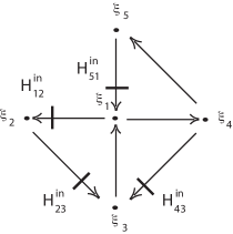
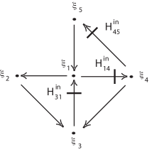
Figure 5: Left: position of the sections in Lemma 4.8. Right: sections in Corollary 4.9.

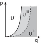
Figure 7: Decomposition for Lemma A.3 in the $(p,q)$ plane. The dashed line, the common boundary of $U^{II}$ and $U^{III}$, is mapped by $h^{II}$ into the solid line, the common boundary of $U^{I}$ and $U^{III}$.

In this section we derive conditions for f.a.s. and calculate stability indices for a cycle that in the quotient space is $[R_{z}\to{\widetilde{PQ}}_{w}\to R_{w}\to R_{z}]$. Three numerical simulations of this cycle appear in Figures 5–7 of [3]. We consider behaviour of trajectories near the cycle that in ${\mathbb{R}}^{6}$ is

$$R_{w}\to R_{z}\to\rho^{2}{\widetilde{PQ}}_{w}\to-\rho R_{w}\qquad\mbox{that is}\qquad\xi_{3}\to\xi_{1}\to\xi_{4}\to-\rho\xi_{3}.$$ (19)

Since the cycle is a part of a network and by assumption equilibria are stable in the transverse directions, the eigenvalues $\lambda_{ij}$ of $df(\xi_{i})$, $i=1,3,4$, satisfy:

$$\begin{array}[]{ll}\lambda_{1j}<0,\ j=1,2,3,4,&\lambda_{4j}<0,\ j=1,4,6,\\ \lambda_{3j}<0,\ j=2,4,5,&\lambda_{15},\lambda_{16},\lambda_{42}=\lambda_{43},\lambda_{45},\lambda_{31}>0.\end{array}$$ (20)

We prove the following theorem:

Theorem 4.2.

Consider the cycle ${\cal C}_{143}$ and assume that the conditions (20) are satisfied. Denote

$$\beta_{1}=\frac{\lambda_{41}\lambda_{35}}{\lambda_{45}\lambda_{31}}(1-\frac{\lambda_{15}}{\lambda_{16}}),\qquad\beta_{2}=-\frac{\lambda_{32}}{\lambda_{31}}+\frac{\lambda_{35}\lambda_{12}}{\lambda_{31}\lambda_{16}}+\frac{\lambda_{35}\lambda_{42}}{\lambda_{31}\lambda_{45}}\left(1-\frac{\lambda_{15}}{\lambda_{16}}\right)$$ (21)

Then

• If

  $$\lambda_{16}<\lambda_{15}\quad\hbox{ or }\quad\beta_{1}+\beta_{2}<1\quad\hbox{ or }\quad\beta_{2}<0,$$

  then the cycle c.u.

• If

  $$\lambda_{16}>\lambda_{15},\quad\beta_{1}+\beta_{2}>1\quad\hbox{ and }\quad\beta_{2}>0$$ (22)

  then the cycle is f.a.s. The stability indices are:

  $$\sigma(\kappa_{43},{\cal C}_{143})=+\infty,$$

  $$\sigma(\kappa_{14},{\cal C}_{143})=\bigg{\{}\begin{array}[]{lll}1-\lambda_{42}/\lambda_{45}&\hbox{ if }&\lambda_{45}>\lambda_{42}\\ \lambda_{45}/\lambda_{42}-1&\hbox{ if }&\lambda_{45}<\lambda_{42}\end{array}$$

  $$\sigma(\kappa_{31},{\cal C}_{123})=\bigg{\{}\begin{array}[]{lll}\min\{1-\lambda_{15}/\lambda_{16},(1+\beta_{3}-\beta_{4})/\beta_{4}\}&\hbox{ if }&\beta_{4}<\beta_{3}+1\\ \min\{1-\lambda_{15}/\lambda_{16},(-1-\beta_{3}+\beta_{4})/\beta_{3},-\beta_{3}+\beta_{4}-1\}&\hbox{ if }&\beta_{4}\geq\beta_{3}+1\end{array}$$

  where

  $$\beta_{3}=-\frac{\lambda_{12}}{\lambda_{16}}+\frac{\lambda_{15}\lambda_{42}}{\lambda_{16}\lambda_{45}},\qquad\beta_{4}=-\frac{\lambda_{42}}{\lambda_{45}}.$$

We begin the proof of the theorem by proving a lemma. Denote by $w(h,\varepsilon,a,b)$, where $0<\varepsilon<h$, $a>0$ and $b>0$, the volume of the set $W\subset{\mathbb{R}}^{3}$,

$$W=\{{\bf x}\in{\mathbb{R}}^{3}~{}:~{}x_{1}x_{2}^{a}>hx_{3}^{b},~{}0\leq x_{j}\leq\varepsilon,\hbox{ for }j=1,2,3~{}\}.$$

Lemma 4.3.

For sufficiently small $\varepsilon>0$ the volume of the set $W$ is

$$w(h,\varepsilon,a,b)=\bigg{\{}\begin{array}[]{lll}C_{1}(h,a,b)\varepsilon^{2+(a+1)/b}&\hbox{ if }&b<1+a\\ C_{2}(h,a,b)\varepsilon^{2+(b-1)/a}+C_{3}(h,a,b)\varepsilon^{2+b-a}&\hbox{ if }&b\geq 1+a\end{array}$$

where $C_{i}(h,a,b)$ are positive constants independent of $\varepsilon$.

Proof.

If $b<1+a$ then for sufficiently small $\varepsilon$ the function $g(x_{1},x_{2})=h^{-1/b}x_{1}^{1/b}x_{2}^{a/b}$ satisfies $g(x_{1},x_{2})<\varepsilon$ for all $0<x_{1}<\varepsilon$ and $0<x_{2}<\varepsilon$. Therefore,

$$w(h,\varepsilon,a,b)=\int_{0}^{\varepsilon}\int_{0}^{\varepsilon}g(x_{1},x_{2}){\rm d}x_{1}{\rm d}x_{2}=\frac{h^{-1/b}b^{2}}{(a+b)(b+1)}\varepsilon^{2+(1+a)/b}.$$

For $b\geq 1+a$ we represent $W=W^{1}\setminus W^{2}$, where

$$\begin{array}[]{l}W^{1}=\{{\bf x}\in{\mathbb{R}}^{3}~{}:~{}0<x_{3}<g(x_{1},x_{2}),~{}0\leq x_{1}\leq\varepsilon,\ 0\leq x_{2}\leq\varepsilon~{}\},\\ W^{2}=\{{\bf x}\in{\mathbb{R}}^{3}~{}:~{}\varepsilon<x_{3}<g(x_{1},x_{2}),~{}0\leq x_{1}\leq\varepsilon,\ 0\leq x_{2}\leq\varepsilon~{}\}.\end{array}$$

Therefore,

$$w(h,\varepsilon,a,b)=\int_{0}^{\varepsilon}\int_{0}^{\varepsilon}g(x_{1},x_{2}){\rm d}x_{1}{\rm d}x_{2}-\int_{h^{-1/b}\varepsilon^{(b-1)/a}}^{\varepsilon}\int_{h\varepsilon^{b}x_{2}^{-a}}^{\varepsilon}g(x_{1},x_{2}){\rm d}x_{1}{\rm d}x_{2}=$$

$$\frac{h^{1/a-1/b}b^{2}}{(a+b)(b+1)}\varepsilon^{2+(b-1)/a}+\frac{hb}{(1-a)(b+1)}\varepsilon^{2+b-a}-\frac{h^{1/a}b}{(1-a)(b+1)}\varepsilon^{2+(b-1)/a}.$$ (23)

∎

Remark 4.4.

For $h\to 0$ in the sum (23) the third term is asymptotically smaller than the first one.

Remark 4.5.

In the limit $\varepsilon\to 0$ for $a>1$ in the sum (23) the first term is asymptotically larger than the second one, while for $a<1$ the second term is asymptotically larger.

Proof of the theorem. Similarly to the proof of Theorem 4.1, we approximate the behaviour of trajectories near the cycle by the return map $\tilde{\bf g}:H_{3}^{{\rm in}}\to H_{3}^{{\rm in}}$. For the cycle ${\cal C}_{143}$ the expression for this map that we derive coincides (up to expressions for coefficients $\beta_{1}$ and $\beta_{2}$) with the one obtained in Theorem 4.1 for the cycle ${\cal C}_{123}$. Hence, we apply results of Appendix A to find conditions for asymptotic stability. Calculation of stability indices for the cycle ${\cal C}_{143}$ is more difficult, because the equilibrium $\xi_{4}$ has a three-dimensional unstable manifold, while the unstable manifold of $\xi_{2}$ is one-dimensional.

The local maps $H^{\rm in}_{j}\to H^{\rm out}_{j}$ are:

$$\begin{array}[]{cl}\phi_{1}:\ H^{\rm in}_{1}\to H^{\rm out}_{1}&u_{12}^{\rm out}=u_{12}^{\rm in}|u_{16}^{\rm in}|^{-\lambda_{12}/\lambda_{16}},\ u_{13}^{\rm out}=u_{13}^{\rm in}|u_{16}^{\rm in}|^{-\lambda_{12}/\lambda_{16}},\\ &u_{14}^{\rm out}=D_{2}|u_{16}^{\rm in}|^{-\lambda_{14}/\lambda_{16}},\ u_{15}^{\rm out}=u_{15}^{\rm in}|u_{16}^{\rm in}|^{-\lambda_{15}/\lambda_{16}}\\ \phi_{4}:\ H^{\rm in}_{4}\to H^{\rm out}_{4}&u_{41}^{\rm out}=D_{3}|u_{45}^{\rm in}|^{-\lambda_{41}/\lambda_{45}},\ u_{42}^{\rm out}=u_{42}^{\rm in}|u_{45}^{\rm in}|^{-\lambda_{42}/\lambda_{45}},\\ &u_{43}^{\rm out}=u_{43}^{\rm in}|u_{45}^{\rm in}|^{-\lambda_{42}/\lambda_{45}},\ u_{44}^{\rm out}=u_{44}^{\rm in}|u_{45}^{\rm in}|^{-\lambda_{44}/\lambda_{45}},\\ \phi_{3}:\ H^{\rm in}_{3}\to H^{\rm out}_{3}&u_{32}^{\rm out}=u_{32}^{\rm in}|u_{31}^{\rm in}|^{-\lambda_{32}/\lambda_{31}},\ u_{33}^{\rm out}=u_{33}^{\rm in}|u_{31}^{\rm in}|^{-\lambda_{32}/\lambda_{31}},\\ &u_{35}^{\rm out}=u_{35}^{\rm in}|u_{31}^{\rm in}|^{-\lambda_{35}/\lambda_{31}},\ u_{36}^{\rm out}=D_{1}|u_{31}^{\rm in}|^{-\lambda_{35}/\lambda_{31}},\\ \end{array}$$ (24)

where $D_{1}$, $D_{2}$ and $D_{3}$ are some positive constants.

The global maps $\psi_{ij}:H^{\rm out}_{i}\to H^{\rm in}_{j}$ are:

$$\begin{array}[]{cl}\psi_{14}:\ H^{\rm out}_{1}\to H^{\rm in}_{4}&u_{42}^{\rm in}=B_{1}u_{12}^{\rm out}+B_{2}u_{13}^{\rm out},\ u_{43}^{\rm in}=B_{3}u_{12}^{\rm out}+B_{4}u_{13}^{\rm out},\\ &\ u_{44}^{\rm in}=B_{5}u_{14}^{\rm out},\ u_{45}^{\rm in}=B_{6}u_{15}^{\rm out}\\ \psi_{43}:\ H^{\rm out}_{4}\to H^{\rm in}_{3}&\hat{u}_{31}^{\rm in}=C_{1}u_{42}^{\rm out}+C_{2}u_{43}^{\rm out},\ \hat{u}_{32}^{\rm in}=C_{3}u_{41}^{\rm out},\\ &\hat{u}_{33}^{\rm in}=C_{4}u_{42}^{\rm out}+C_{5}u_{43}^{\rm out},\ \hat{u}_{35}^{\rm in}=C_{6}u_{44}^{\rm out}\\ \psi_{31}:\ H^{\rm out}_{3}\to H^{\rm in}_{1}&u_{12}^{\rm in}=A_{1}\tilde{u}_{32}^{\rm out},\ u_{13}^{\rm in}=A_{2}\tilde{u}_{33}^{\rm out},\\ &u_{15}^{\rm in}=A_{3}\tilde{u}_{35}^{\rm out},\ u_{16}^{\rm in}=A_{4}\tilde{u}_{36}^{\rm out},\end{array}$$ (25)

where $A_{j}$, $B_{j}$, $C_{3}$ and $C_{6}$ are positive. To complete the return map $\tilde{\bf g}:H^{\rm in}_{3}\to H^{\rm in}_{3}$ one should apply the change of coordinates (18) between $\psi_{43}$ and $\phi_{3}$.

Note the similarity of expressions (24) and (25) with the ones (16) and (17). Here $\psi_{14}$ differs slightly from $\psi_{12}$, but this does not modify the final expression for superposition. Hence, we can apply results of Appendix A about stability of the map $\tilde{\bf g}$. For the ${\cal C}_{143}$ cycle the conditions for stability take the form

• If

  $$\lambda_{16}<\lambda_{15},\quad\hbox{ or }\quad\beta_{1}<0,\quad\hbox{ or }\quad\beta_{2}<0,\quad\hbox{ or }\quad\beta_{1}+\beta_{2}<1,$$

  then the origin is a completely unstable fixed point of the map $\tilde{\bf g}$.

• If

  $$\lambda_{16}>\lambda_{15},\quad\beta_{1}>0,\quad\beta_{2}>0\quad\hbox{ and }\quad\beta_{1}+\beta_{2}>1,$$

  then the origin is an asymptotically stable fixed point of the map $\tilde{\bf g}$.

Statement (i) holds true, because instability of $\tilde{\bf g}$ implies instability of the cycle. Below we prove (ii). The stability properties of the cycle are studied by calculating stability indices along the connections, as it was done in the proof of Theorem 4.1.

Since $\beta_{1}>0$, the inequalities (22) imply that the origin is an a.s. fixed point of the map $\tilde{\bf g}$. Consider ${\bf x}\in H^{\rm in}_{3}({\varepsilon})$, i.e. $|{\bf x}|<\varepsilon$. For almost all ${\bf x}$ (i.e., except the points that belong to the stable manifolds of the equilibria), the trajectory $\Phi_{t}({\bf x})$ starting at ${\bf x}$ follows the connection $\kappa_{31}$ and then $\kappa_{14}$, the latter happens since $\lambda_{16}>\lambda_{15}$. Then, the trajectory follows the connection $\kappa_{42}$, because the map $(\psi_{43})^{-1}\tilde{\bf g}:H_{3}^{{\rm in}}\to H_{4}^{{\rm out}}$ is a superposition of a linear map and an asymptotically stable $\tilde{\bf g}$. By the same arguments as employed in the proof of Theorem 4.1, the trajectory stays close to the cycle for all positive $t$, hence $\sigma(\kappa_{43},{\cal C}_{143})=+\infty$.

For ${\bf u}\in H^{\rm in}_{4}$, ${\bf u}=\left(u_{42},u_{43},u_{44},u_{45}\right)$, the trajectories $\Phi_{t}({\bf u})$ that escape the $\delta$-neighbourhood of $\xi_{4}$ along the connection $\kappa_{43}$ satisfy

$$u_{42}u_{45}^{-\lambda_{42}/\lambda_{45}}<\delta\hbox{ and }u_{43}u_{45}^{-\lambda_{42}/\lambda_{45}}<\delta.$$ (26)

Then, they are mapped by $\psi_{43}$ to $H_{3}^{{\rm in}}$ and, given that $|{\bf u}|$ is sufficiently small, stay close to the cycle for all $t>0$, as proven above. The stability index can be positive or negative, depending on the sign of $\lambda_{42}-\lambda_{45}$. Calculating the measure of the area bounded by (26), we obtain that the index is $1-\lambda_{42}/\lambda_{45}$ for $\lambda_{45}>\lambda_{42}$ and $\lambda_{45}/\lambda_{42}-1$ for $\lambda_{45}<\lambda_{42}$.

In $H^{\rm in}_{1}$ the trajectories that escape a $\delta$-neighbourhood of $\xi_{1}$ along the connection $\kappa_{14}$ satisfy $u_{15}u_{16}^{-\lambda_{15}/\lambda_{16}}<\delta$. By substituting the expressions for $\phi_{1}$ and $\psi_{14}$ into $\phi_{4}$ (see (24) and (25)), we obtain that trajectories that escape a $\delta$-neighbourhood of $\xi_{4}$ along the connection $\kappa_{43}$ satisfy

$$pu_{16}^{\beta_{3}}u_{15}^{\beta_{4}}<\delta,$$ (27)

where $p=\max\{|x_{12}|,|x_{13}|\}$ and $\beta_{3}$ and $\beta_{4}$ are the ones given in the statement of the theorem. The measure of the set (27) is calculated in Lemma 4.3. Applying the definition of stability indices, we complete the proof of (ii). ∎

Corollary 4.6.

Consider the cycle ${\cal C}_{143}$ of Theorem 4.2. Then:

• If (22) holds and in addition the inequality $\lambda_{45}>\lambda_{42}$ holds true then the cycle is e.a.s.

• If $\lambda_{45}<\lambda_{42}$ then the cycle is not e.a.s.

Proof. To prove (iii) and (iv), we note that the only stability index that can be non-positive is $\sigma(\kappa_{14},{\cal C}_{143})$. If $\lambda_{45}>\lambda_{42}$ then the index is positive and, hence, the cycle is e.a.s. If $\lambda_{45}<\lambda_{42}$ then the index is negative and, hence, the cycle is not e.a.s. ∎

4.2.3 The cycle ${\cal C}_{145}=[R_{z}\to{\widetilde{PQ}}_{w}\to PQ_{z}\to R_{z}]$

In this section we are concerned with the cycle $[R_{z}\to\rho^{2}{\widetilde{PQ}}_{w}\to\rho^{2}PQ_{z}\to\rho^{2}R_{z}]$, that is $\xi_{1}\to\xi_{4}\to\xi_{5}\to\rho^{2}\xi_{1}$. This cycle is pseudo-simple (see [19, Definition 5]) because there is a two-dimensional isotypic component corresponding to the expanding eigenspace of $\xi_{4}$. For the same reason this cycle is completely unstable, as we show in the next theorem. In [3] no numerical simulations show trajectories that stayed close to this cycle.

Theorem 4.7.

Generically, the cycle ${\cal C}_{145}$ is completely unstable.

Proof.

The proof is similar to the proof of Theorem 1 in [19]. We consider the map $\phi_{4}\psi_{14}\phi_{1}:H^{\rm in}_{1}\to H^{\rm out}_{4}$ where $\phi_{4}$ and $\phi_{1}$ are the local maps around $\xi_{4}$ and $\xi_{1}$, respectively and $\psi_{14}$ is the global map along the connection $\kappa_{14}$.

The local maps are:

$$\begin{array}[]{cl}\phi_{1}:\ H^{\rm in}_{1}\to H^{\rm out}_{1}&u_{12}^{\rm out}=D_{1}|u_{16}^{\rm in}|^{-\lambda_{12}/\lambda_{16}},\ u_{13}^{\rm out}=u_{13}^{\rm in}|u_{16}^{\rm in}|^{-\lambda_{12}/\lambda_{16}},\\ &u_{14}^{\rm out}=u_{14}^{\rm in}|u_{16}^{\rm in}|^{-\lambda_{14}/\lambda_{16}},\ u_{15}^{\rm out}=u_{15}^{\rm in}|u_{16}^{\rm in}|^{-\lambda_{15}/\lambda_{16}}\\ \phi_{4}:\ H^{\rm in}_{4}\to H^{\rm out}_{4}&u_{41}^{\rm out}=D_{2}|u_{42}^{\rm in}|^{-\lambda_{41}/\lambda_{42}},\ u_{43}^{\rm out}=u_{43}^{\rm in}|u_{42}^{\rm in}|^{-\lambda_{43}/\lambda_{42}},\\ &u_{44}^{\rm out}=u_{44}^{\rm in}|u_{42}^{\rm in}|^{-\lambda_{44}/\lambda_{42}},\ u_{45}^{\rm out}=u_{45}^{\rm in}|u_{42}^{\rm in}|^{-\lambda_{45}/\lambda_{42}}\end{array}$$ (28)

where $D_{1}$, $D_{2}$ are some positive constants. The expression for the global map $\psi_{14}$ is given in (25).

For small values of ${\bf u}$, the coordinate $u_{13}^{\rm out}$ in the expression for $\phi_{1}$ is much smaller than $u_{12}^{\rm out}$. Thus, when computing $\psi_{14}\phi_{1}$ the second terms in the sums $B_{1}u_{12}^{\rm out}+B_{2}u_{13}^{\rm out}$ and $B_{3}u_{12}^{\rm out}+B_{4}u_{13}^{\rm out}$ may be ignored. Because $\lambda_{43}=\lambda_{42}$ the coordinate $u_{43}^{\rm out}$ in $\phi_{4}$ may be rewritten as $u_{43}^{\rm out}=u_{43}^{\rm in}|u_{42}^{\rm in}|^{-1}$. Therefore in the final superposition, one obtains $u_{43}^{\rm out}\approx B_{3}/B_{1}$. Since generically $B_{3}\neq 0$ the term $u_{43}^{\rm out}$ cannot be made arbitrarily small. ∎

4.3 The network

In this section $\Sigma$ denotes the network, $H_{ij}^{\rm in}$ denotes a cross-section to the connection $\kappa_{ij}$ close to the node $\xi_{j}$ and $H_{ij}^{\rm out}$ is a cross-section to the connection $\kappa_{ij}$ close to the node $\xi_{i}$. We also use the more cumbersome notation $\phi_{ijk}:H_{ij}^{\rm in}\rightarrow H_{jk}^{\rm out}$ for what was denoted $\phi_{j}$ above, to emphasise the connections $\kappa_{ij}$ and $\kappa_{jk}$ that are being followed.

A necessary condition for existence of the network and its stability in the transverse directions is that eigenvalues $\lambda_{ij}$ satisfy

$$\begin{array}[]{lcl}\lambda_{1j}<0,\ j=1,2,3,4,&&\lambda_{2j}<0,\ j=1,2,3,4,5,\\ \lambda_{3j}<0,\ j=2,4,5,&&\lambda_{4j}<0,\ j=1,4,6,\\ \lambda_{5j}<0,\ j=1,2,4,5,6&&\lambda_{15},\lambda_{16},\lambda_{26},\lambda_{31},\lambda_{42}=\lambda_{43},\lambda_{45},\lambda_{53}>0.\end{array}$$ (29)

Lemma 4.8.

If both cycles ${\cal C}_{123}$ and ${\cal C}_{143}$ are c.u. and $\lambda_{15}>\lambda_{16}$ then for $\delta>0$ sufficiently small, we have $\ell\left(H_{ij}^{\rm in}\cap{\cal B}_{\delta}(\Sigma)\right)=0$, for $ij\in\{12,23,43,51\}$, where $\ell$ denotes the Lebesgue measure in ${\mathbb{R}}^{n}$ with $n=\dim H_{ij}^{\rm in}$.

Proof.

We do the proof for $H_{23}^{\rm in}$, the cases $H_{12}^{\rm in}$ and $H_{43}^{\rm in}$ are similar. Let ${\bf u}\in H_{23}^{\rm in}\cap{\cal B}_{\delta}(\Sigma)$. Consider the transition map $H_{23}^{\rm in}\to H_{31}^{\rm in}$, denoted by $\tilde{{\bf g}}^{(3)}$ in Lemma A.1. The estimate (34) shows that $\tilde{{\bf g}}^{(3)}({\bf u})$ satisfies $u_{16}^{\rm in}\approx Cu_{15}^{\rm in}$ for some nonzero constant $C$. If the trajectory of ${\bf u}$ follows the connection $\kappa_{14}$ after passing near $\xi_{1}$, then from the expression (24) for the local map $\phi_{1}$ and the estimate above, we get

$$u_{15}^{\rm out}=u_{15}^{\rm in}|u_{16}^{\rm in}|^{-\lambda_{15}/\lambda_{16}}\approx C|u_{15}^{\rm in}|^{1-\lambda_{15}/\lambda_{16}}.$$

Since $1-\lambda_{15}/\lambda_{16}<0$, we have $\displaystyle\lim_{\delta\to 0}u_{15}^{\rm out}=\infty$. Hence, if the trajectory of ${\bf u}$ follows $\kappa_{14}$ then ${\bf u}\not\in{\cal B}_{\delta}(\Sigma)$ for sufficiently small $\delta$. Therefore, the set $H_{23}^{\rm in}\cap{\cal B}_{\delta}(\Sigma)$ is contained in the set $H_{23}^{\rm in}\cap{\cal B}_{\delta}({\cal C}_{123})$ that, for sufficiently small $\delta$, has zero measure.

For $H_{51}^{\rm in}$, we use $\ell\left(H_{43}^{\rm in}\cap{\cal B}_{\delta}(\Sigma)\right)=0$ and apply similar arguments recalling that by Theorem 4.7 the cycle ${\cal C}_{145}$ is c.u. ∎

Corollary 4.9.

Under the conditions of Lemma 4.8 and for $\delta>0$ sufficiently small we have $\ell\left(H_{ij}^{\rm in}\cap{\cal B}_{\delta}(\Sigma)\right)=0$, for $ij\in\{45,14,31\}$.

Proof.

Except for a measure zero set, trajectories starting in $H_{45}^{\rm in}$ go to $H_{51}^{\rm in}$, where we can apply the result of Lemma 4.8. Similarly, most trajectories starting in $H_{14}^{\rm in}$ either follow $\kappa_{45}$ or $\kappa_{43}$. Those following $\kappa_{43}$ end up mostly in $H_{43}^{\rm in}$, and those near $\kappa_{45}$ end up mostly in $H_{45}^{\rm in}$, and both these sets meet ${\cal B}_{\delta}(\Sigma)$ in a measure zero set. The arguments for $H_{31}^{\rm in}$ are entirely similar. ∎

Theorem 4.10.

Generically for the network $\Sigma$:

• At most one of the cycles ${\cal C}_{123}$ or ${\cal C}_{143}$ is f.a.s.

• The network is f.a.s. whenever one of the cycles is f.a.s.

Proof.

• If $\lambda_{16}>\lambda_{15}$ then Theorem 4.1 implies that if ${\cal C}_{123}$ is c.u. whereas if $\lambda_{15}>\lambda_{16}$ then ${\cal C}_{143}$ is c.u. by Theorem 4.2.

• Clearly, if one of the cycles is f.a.s. then the network is f.a.s. It remains to see that when both cycles are c.u. then the network is not f.a.s. If $\lambda_{15}>\lambda_{16}$ this is a consequence of Lemma 4.8 and its corollary.

  The proof in the case $\lambda_{16}>\lambda_{15}$ is postponed till after we obtain a few lemmas.

Lemma 4.11.

Consider the map $g^{\prime}:H_{43}^{\rm in}\rightarrow H_{45}^{\rm out}$ given by $g^{\prime}=\phi_{145}\psi_{14}\phi_{314}\psi_{31}\phi_{431}$ (see Figure 6). The points in $H_{43}^{\rm in}$ that are mapped by $g^{\prime}$ into $V_{\delta}\cap H_{45}^{\rm out}$, for sufficiently small $\delta>0$ belong to the set

$$V_{45}=\left\{{\bf u}\in H_{43}^{\rm in}:\ \left(B_{3}^{\prime}u_{32}^{\rm in}+B_{4}^{\prime}u_{33}^{\rm in}\right)<\delta c^{\prime}\max\left(|u_{32}^{\rm in}|,|u_{33}^{\rm in}|\right)\right\}$$

where $B_{3}^{\prime}$, $B_{4}^{\prime}$ and $c^{\prime}$ are constants, independent on $\delta$.

Proof.

A direct computation using (28) for $\phi_{145}$ and (24) and (25) for the remaining maps, shows that writing $g^{\prime}({\bf u})=\left(u_{41}^{\rm out},u_{42}^{\rm out},u_{43}^{\rm out},u_{44}^{\rm out}\right)$ we have

$$u_{43}^{\rm out}=\left(B_{1}^{\prime}u_{32}^{\rm in}+B_{2}^{\prime}u_{33}^{\rm in}\right)^{-1}\left(B_{3}^{\prime}u_{32}^{\rm in}+B_{4}^{\prime}u_{33}^{\rm in}\right)$$

∎

The next lemma follows immediately from Lemmas 3.8 and 3.9.

Lemma 4.12.

Let ${\bf h}(p,q)$ be one of the maps considered in Lemmas 3.8 and 3.9. For given $(p,q)=(r^{a},r^{b})$ we define $a_{n}$, $b_{n}$ by ${\bf h}^{n}(r^{a},r^{b})=(r^{a_{n}},b^{b_{n}})$. For any $a>0$, $b>0$ and $s>0$ there exists $0<n_{0}<\infty$ such that $\min\{a_{n},b_{n}\}>0$ for all $n>n_{0}$ and at least one of the following is satisfied:

• $\min\{a_{n_{0}},b_{n_{0}}\}\leq 0$;

• $\gamma-s<a_{n}/b_{n}<\gamma+s$ for all $n=n^{\prime}+2m>n_{0}$;

• $v_{1}^{+}/v_{2}^{+}-s<a_{n}/b_{n}<v_{1}^{+}/v_{2}^{+}+s$ for all $n>n_{0}$;

where $\gamma$, $v_{1}^{+}$ and $v_{2}^{+}$ take the meanings they have in Lemmas 3.8 and 3.9.

Lemma 4.13.

Consider the map $\tilde{{\bf g}}:H_{43}^{\rm in}\rightarrow H_{43}^{\rm in}$ in the proof of Theorem 4.2. Let $W\subset H_{43}^{\rm in}$ satisfy

$$W\subset\left\{{\bf u}=(u_{31}^{\rm in}=q,u_{32}^{\rm in},u_{33}^{\rm in},u_{35}^{\rm in}):\quad a_{j}q^{\gamma_{j}}<u_{3j}^{\rm in}<b_{j}q^{\gamma_{j}}\quad j=2,3\right\}$$

where $a_{j}b_{j}>0$, $\gamma_{j}>0$ and $\gamma_{2}\neq\gamma_{3}$. Then, for sufficiently small $\varepsilon>0$, any point $\hat{\bf u}=\tilde{\bf g}({\bf u})=(\hat{u}_{31}^{\rm in}=\hat{q},\hat{u}_{32}^{\rm in},\hat{u}_{33}^{\rm in},\hat{u}_{35}^{\rm in})\in\tilde{\bf g}(W\cap V_{\varepsilon})$ satisfies

$$\hat{a}_{j}\hat{q}^{\hat{\gamma}_{j}}<\hat{u}_{3j}^{\rm in}<\hat{b}_{j}\hat{q}^{\hat{\gamma}_{j}}\quad j=2,3$$

where $\hat{a}_{j}\hat{b}_{j}>0$ are independent on $\varepsilon$, $\hat{\gamma}_{3}=1$ and $\displaystyle\hat{\gamma}_{2}=\frac{\beta_{1}}{\min\{\gamma_{2},\gamma_{3}\}+\beta_{2}}$.

Proof.

Follows from Lemma A.1 and from the expressions (34) and (36). ∎

Corollary 4.14.

Generically, the statement of Lemma 4.13 holds if $\tilde{\bf g}$ is replaced by $\tilde{\bf g}^{n}$ for any finite $n>0$, with a different $\hat{\gamma}_{2}$.

Definition 4.15.

We say that a set $V\subset{\mathbb{R}}^{4}$ is conical with exponents $(1,\gamma_{2},\gamma_{3},\gamma_{4})$, $\gamma_{j}>0$, if

$$V\subset\left\{(x_{1},x_{2},x_{3},x_{4})\in{\mathbb{R}}^{4}:\quad a_{j}x_{1}^{\gamma_{j}}<x_{j}<b_{j}x_{1}^{\gamma_{j}},\ j=,2,3,4\quad\mbox{where}\quad a_{j}b_{j}>0\right\}.$$

Lemma 4.16.

Generically all our maps ${\bf g}:H_{ij}^{\rm in}\rightarrow H_{k\ell}^{\rm in}$ have the following property: if an initial set $U\subset H_{ij}^{\rm in}$ is conical then for sufficiently small $\varepsilon>0$ the image ${\bf g}(U\cap V_{\varepsilon})$ is also conical.

Proof.

The property holds generically for each one of the local and global maps. Hence, it also holds for compositions of these maps. ∎

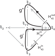
Figure 6: The maps ${\bf g}^{\prime}$ and ${\bf g}^{\prime\prime}$ of Lemmas 4.11 and 4.17, with the network shown in grey.

Lemma 4.17.

Denote $\hat{\bf g}={\bf g}^{\prime\prime}{\bf g}^{\prime}$ where ${\bf g}^{\prime\prime}:H_{45}^{\rm out}\rightarrow H_{14}^{\rm in}$ is given by ${\bf g}^{\prime\prime}=\psi_{14}\phi_{514}\psi_{51}\phi_{451}\psi_{45}$ and ${\bf g}^{\prime}$ was defined in Lemma 4.11 (see Figure 6). Let $U_{45}\subset H_{43}^{\rm in}\cap{\cal B}_{\delta}(\Sigma)$ be the subset that is mapped to $H_{45}^{\rm out}$ by ${\bf g}^{\prime}$. For any $c_{0}>0$ and sufficiently small $\varepsilon>0$ there is a set $W_{c_{0}}$ such that the image $\hat{\bf g}\left((U_{45}\setminus W_{c_{0}})\cap V_{\varepsilon}\right)$ is conical with exponents $(1,1,\lambda_{16}-\lambda_{14},\lambda_{16}-\lambda_{15})$. The set $W_{c_{0}}$ is defined by

$$W_{c_{0}}=\left\{\left|L_{j1}rq^{-1}+L_{j2}p^{\gamma_{1}}q^{\gamma_{2}}+L_{j3}p^{\gamma_{3}}q^{\gamma_{4}}\right|<c_{0}\max\left\{|rq^{-1}|,|p^{\gamma_{1}}q^{\gamma_{2}}|,|p^{\gamma_{3}}q^{\gamma_{4}}|\right\}\ \ j=1,2,3\right\}$$

where $q=u_{31}^{\rm in}$, $p=u_{32}^{\rm in}$, $r=B_{3}^{\prime}u_{32}^{\rm in}+B_{4}^{\prime}u_{33}^{\rm in}$ and $L_{ji}$,$i,j=1,2,3$, $\gamma_{j}$, $j=1,2,3,4$ and $B_{3}^{\prime}$, $B_{4}^{\prime}$ are constants coming from the expressions for global and local maps.

Proof.

Let ${\bf u}\in H_{45}^{\rm in}$ be given by ${\bf u}=(u_{51}^{\rm in},u_{53}^{\rm in},u_{54}^{\rm in},u_{55}^{\rm in})$. The coordinates $u_{5j}^{\rm in}$, $j=3,4,5$ for the map $\psi_{45}:H_{45}^{\rm in}:\rightarrow H_{45}^{\rm out}$ have the form

$$u_{5j}^{\rm in}=L_{j-2,1}^{\prime}u_{43}^{\rm out}+L_{j-2,2}^{\prime}u_{44}^{\rm out}+L_{j-2,3}^{\prime}u_{45}^{\rm out}\qquad j=3,4,5.$$

This implies that the composition $\psi_{45}{\bf g}^{\prime}:H_{43}^{\rm in}\rightarrow H_{45}^{\rm in}$, in terms of $p$, $q$, $r$ satisfies

$$u_{5,j+2}^{\rm in}=L_{j1}rq^{-1}+L_{j2}p^{\gamma_{1}}q^{\gamma_{2}}+L_{j3}p^{\gamma_{3}}q^{\gamma_{4}}\qquad j=1,2,3.$$

If $(p,q,r)$ satisfies

$$\left|L_{j1}rq^{-1}+L_{j2}p^{\gamma_{1}}q^{\gamma_{2}}+L_{j3}p^{\gamma_{3}}q^{\gamma_{4}}\right|\geq c_{0}\max\left\{|rq^{-1}|,|p^{\gamma_{1}}q^{\gamma_{2}}|,|p^{\gamma_{3}}q^{\gamma_{4}}|\right\}\quad j=1,2,3$$ (30)

there exist $a_{j}$, $b_{j}$ =, $j=1,2$ such that

$$a_{1}|u_{53}^{\rm in}|<|u_{54}^{\rm in}|<b_{1}|u_{53}^{\rm in}|\qquad\qquad a_{2}|u_{53}^{\rm in}|<|u_{55}^{\rm in}|<b_{2}|u_{53}^{\rm in}|.$$

By writing expressions for $\phi_{415}$ and $\psi_{51}$ and proceeding as above, it can be shown that if $(p,q,r)$ satisfies (30) then for ${\bf u}\in H_{51}^{\rm in}$ there are $a_{j}^{\prime}$, $b_{j}^{\prime}$ =, $j=1,2$ such that we have

$$a_{1}^{\prime}|u_{14}^{\rm in}|<|u_{15}^{\rm in}|<b_{1}^{\prime}|u_{14}^{\rm in}|\qquad\qquad a_{2}^{\prime}|u_{14}^{\rm in}|<|u_{16}^{\rm in}|<b_{2}^{\prime}|u_{14}^{\rm in}|.$$

Using the expressions (25) for $\phi_{514}$ and (28) for $\phi_{14}$ we obtain the exponent
$(1,1,\lambda_{16}-\lambda_{14},\lambda_{16}-\lambda_{15})$ of the statement. ∎

End of proof of Theorem 4.10. In the case $\lambda_{16}>\lambda_{15}$, from Lemmas 4.11, 4.12, 4.13, 4.16 and Corollary 4.14 it follows that, for sufficiently small $\varepsilon>0$ almost all trajectories starting in

$$\hat{\bf g}\left((U_{45}\setminus W_{c_{0}})\cap V_{\varepsilon}\right),$$

after making one turn around ${\cal C}_{145}$, never again leave the $\delta$-neighbourhood of ${\cal C}_{143}$. If we take $c_{0}>0$ small and for small $\varepsilon>0$, we may treat $W_{c_{0}}$ as in Appendix A to show that almost all trajectories that remain close to the network are attracted to the cycle ${\cal C}_{143}$. Since this cycle is not f.a.s. this implies that the set of these trajectories has zero measure, i.e. that for small $\delta>0$ we have $\ell\left(H_{43}^{\rm in}\cap{\cal B}_{\delta}(\Sigma)\right)=0$.

The proof for the other cross-sections follows arguments similar to those in Lemma 4.8 and its corollary. ∎

Theorem 4.18.

Consider the network $\Sigma$ and assume that the eigenvalues $\lambda_{ij}$ satisfy the inequalities (29). Then

• suppose the conditions (15) hold.

  • If $\lambda_{45}<\lambda_{42}$ then $\Sigma$ is not e.a.s.

  • If $\lambda_{45}>\lambda_{42}$ then $\Sigma$ is e.a.s.

• suppose the conditions (22) hold.

  • If $\lambda_{45}<\lambda_{42}$ then $\Sigma$ is not e.a.s.

  • If $-\lambda_{12}\lambda_{45}+\lambda_{15}\lambda_{42}<\lambda_{16}\lambda_{42}$ then $\Sigma$ is not e.a.s.

  • If $\lambda_{45}>\lambda_{42}$ and $-\lambda_{12}\lambda_{45}+\lambda_{15}\lambda_{42}>\lambda_{16}\lambda_{42}$ then $\Sigma$ is e.a.s.

Proof.

Let $V_{\varepsilon}$ be an $\varepsilon$-neighbourhood of the origin. Note that at $\xi_{4}$ there are three outgoing connections: one to $\xi_{3}$, one to $\xi_{5}$, and another to $\gamma_{\pi}^{2}\xi_{5}$.

(ia) Let $\lambda_{42}>\lambda_{45}$. Consider the set $Q_{\varepsilon}\subset H_{14}^{\rm in}$ defined as $Q_{\varepsilon}=\left(H_{14}^{\rm in}\cap{\cal B}_{\delta}(\Sigma)\right)\cap V_{\varepsilon}$. The set can be decomposed as the union $Q_{\varepsilon}=Q_{42}\cup Q_{43}\cup Q_{45}$, such that trajectories from $Q_{4j}$ leave the $\delta$-neighbourhood of $\xi_{4}$ along the connection tangent to ${\bf e}_{4j}$. The sets $Q_{4j}$ satisfy

$$\begin{array}[]{l}Q_{42}\subset\{~{}(u_{42}^{\rm in},u_{43}^{\rm in},u_{44}^{\rm in},u_{45}^{\rm in})~{}:~{}u_{43}^{\rm in}<\delta u_{42}^{\rm in}\hbox{ and }u_{45}^{\rm in}<\delta(u_{42}^{\rm in})^{\lambda_{45}/\lambda_{42}}~{}\}\\ Q_{43}\subset\{~{}(u_{42}^{\rm in},u_{43}^{\rm in},u_{44}^{\rm in},u_{45}^{\rm in})~{}:~{}u_{42}^{\rm in}<\delta u_{43}^{\rm in}\hbox{ and }u_{45}^{\rm in}<\delta(u_{43}^{\rm in})^{\lambda_{45}/\lambda_{42}}~{}\}\\ Q_{45}\subset\{~{}(u_{42}^{\rm in},u_{43}^{\rm in},u_{44}^{\rm in},u_{45}^{\rm in})~{}:~{}u_{43}^{\rm in}<\delta(u_{45}^{\rm in})^{\lambda_{42}/\lambda_{45}}\hbox{ and }u_{42}^{\rm in}<\delta(u_{45}^{\rm in})^{\lambda_{42}/\lambda_{45}}~{}\}.\end{array}$$ (31)

From inclusions (31) we obtain that measures of the sets satisfy

$$\ell(Q_{42})<\frac{1}{2}\delta\varepsilon^{4},\quad\ell(Q_{43})<\frac{1}{2}\delta\varepsilon^{4},\quad\ell(Q_{45})<\frac{\delta\lambda_{42}}{\lambda_{42}+\lambda_{45}}\varepsilon^{3+\lambda_{42}/\lambda_{45}}.$$

Hence, for sufficiently small $\varepsilon$ we have $\ell(Q_{\varepsilon})<2\delta\varepsilon^{4}$, which according to Definition 2.3 implies that $\Sigma$ is not e.a.s.

(ib) Suppose that $\lambda_{42}<\lambda_{45}$. From conditions (15) it follows (see the proof of Theorem 4.2) that $\sigma(\kappa_{12},\Sigma)=\sigma(\kappa_{23},\Sigma)=+\infty$ and $\sigma(\kappa_{12},\Sigma)>0$. Arguments similar to those applied in the proof of Theorem 4.2 imply that $\sigma(\kappa_{43},\Sigma)=+\infty$ and $\sigma(\kappa_{51},\Sigma)\geq\lambda_{15}/\lambda_{16}-1>0$. Calculating the measure of the set $Q_{45}$ constructed above, we obtain that $\sigma(\kappa_{14},\Sigma)\geq\lambda_{45}/\lambda_{42}-1>0$.

To estimate $\sigma(\kappa_{45},\Sigma)$, we introduce the set $W_{\varepsilon}\subset H_{45}^{\rm in}\cap V_{\varepsilon}$ comprised of the points ${\bf u}=(u_{51}^{\rm in},u_{53}^{\rm in},u_{54}^{\rm in},u_{55}^{\rm in})\in H_{45}^{\rm in}$ that are mapped by $\phi_{514}\psi_{51}\phi_{451}$ to $H_{12}^{\rm in}$. The coordinates of these points satisfy

$$\begin{array}[]{l}|L^{\prime}_{31}u_{54}^{\rm in}|u_{53}^{\rm in}|^{-\lambda_{54}/\lambda_{53}}+L^{\prime}_{32}u_{55}^{\rm in}|u_{55}^{\rm in}|^{-\lambda_{55}/\lambda_{53}}+L^{\prime}_{33}C|u_{55}^{\rm in}|^{-\lambda_{56}/\lambda_{53}}|<\\ \delta|L^{\prime}_{21}u_{54}^{\rm in}|u_{53}^{\rm in}|^{-\lambda_{54}/\lambda_{53}}+L^{\prime}_{22}u_{55}^{\rm in}|u_{55}^{\rm in}|^{-\lambda_{55}/\lambda_{53}}+L^{\prime}_{23}C|u_{55}^{\rm in}|^{-\lambda_{56}/\lambda_{53}}|^{\lambda_{16}/\lambda_{15}}\end{array}$$ (32)

(Here $L^{\prime}_{ij}$ and $C$ are the constants of the maps $\psi_{51}$ and $\phi_{451}$, respectively.) By straightforward but lengthy integration (similar to the one in the proof of Lemma 4.3, but significantly longer and with bulky final result), it can be shown that the measure of the set $W_{\varepsilon}$ satisfies $\ell(W_{\varepsilon})>\varepsilon^{4}-\delta\varepsilon^{3+s}$, where $s>1$ depends of the exponents $\lambda_{ij}$ that are involved in (32). Hence, $\sigma(\kappa_{45},\Sigma)>0$ and part (ib) is proven.

The proof of (iia) is identical to the proof of (ia). To prove (iib), we note that the points in $H_{51}^{\rm in}$ that are mapped by $\phi_{341}\psi_{14}\phi_{415}$ to $H_{43}^{\rm out}$ satisfy

$$D|u_{16}^{\rm in}|^{\lambda_{12}/\lambda_{16}}<\delta|u_{15}^{\rm in}(u_{16}^{\rm in})^{\lambda_{15}/\lambda_{16}}|^{\lambda_{42}/\lambda_{45}}.$$

As it is shown in the proof of Theorem 4.7, the points in $H_{51}^{\rm in}$ that are mapped neither to $H_{12}^{\rm out}$ by $\phi_{512}$ nor to $H_{43}^{\rm out}$ by $\phi_{341}\psi_{14}\phi_{415}$, escape from the $\delta$-neghbourhood of the cycle. Hence,

$$\sigma(\kappa_{52},\Sigma)\leq\max\{\lambda_{15}/\lambda_{16}-1,-\lambda_{12}\lambda_{45}/\lambda_{16}\lambda_{42}+\lambda_{15}/\lambda_{16}-1\}<0.$$

The proof of (iic) is similar to the proof of (ib) and is omitted. ∎

5 Conclusion

We complete the study of stability of the heteroclinic network emerging in an ODE obtained from the equations of Boussinesq convection by the center manifold reduction [3]. We derive and prove conditions for fragmentary asymptotic stability and essential asymptotic stability for the network and individual cycles it is comprised of.

This is the first systematic study of stability of heteroclinic cycles that are not of type A or a generalisation of type Z (see [6] for the latter). Although we consider a particular case study, the proposed approach consisting of well-defined steps is applicable to other heteroclinic cycles in ${\mathbb{R}}^{n}$. Moreover, some of the lemmas that we prove are not restricted to the case under investigation and can become useful in other systems.

The study of stability of heteroclinic networks is less common than that of heteroclinic cycles. It requires the construction and composition of several transition maps between cross-sections to connections belonging to different cycles. This procedure is likely to work for other networks as well.

Our results show that derivation of general stability conditions for heteroclinic cycles in ${\mathbb{R}}^{n}$ with $n\geq 6$ is a highly non-trivial task, if at all possible. It would be of interest to identify classes of heteroclinic cycles for which derivation of stability conditions is possible. To do so, one should somehow classify possible maps $h$ obtained at step (b) discussed in the introduction. The classification (at least, partial) should start with determining possible forms of the map $h$.

In Section 3 we prove Theorem 3.1 stating necessary conditions for a heteroclinic network to be asymptotically stable. Corollary 3.2 of this theorem implies that the network under investigation in not asymptotically stable. The theorem can be used to prove instability of more general types of heteroclinic networks, than considered in the Corollary, in particular, with (some of) the equilibria replaced by periodic orbits. We intend to address this question in the future.

For heteroclinic cycles the stability indices provide quantitative and qualitative description for behaviour of nearby trajectories. In a f.a.s. heteroclinic network the trajectory through a point that belongs to its local basin can be possibly attracted by any of its f.a.s. subcycles, or it can switch between different subcycles, without being attracted by any of them. Certainly, stability indices, either for the whole network or for individual cycles, do not provide such information. One can think about proposing for a network $X$, a subset $Y\subset X$ and a point $x\in X$ a relative stability index $\sigma(x,Y,X)$, describing the part of a small neighbourhood of $x$ that stays near $X$ for all $t>0$ and is attracted by $Y$ as $t\to\infty$. If in addition the sets $Y$ are required to be maximal and undecomposable, such relative stability indices should be useful for describing local dynamics near the network. Introduction of such an index is beyond the scope of the present paper. A step toward this direction was made in [4] by defining stability indices with respect to a cycle (the $c$-index) and with respect to the whole network (the $n$-index).

Appendix A Lemmas in the proof of Theorem 4.1

Denote by $\tilde{g}_{j}^{(k)}$ , where $j=1,2,3,4$, the $j$-th component of the map $\psi_{ki}\phi_{k}$, with $i=k+1\pmod{3}$.

Lemma A.1.

For any $\delta>0$ there exist $\varepsilon>0$ such that $|{u}_{35}^{\rm in}|<\varepsilon$ implies that

$$(i)\qquad|A_{4}\tilde{g}_{3}^{(3)}({u}_{31}^{\rm in},{u}_{32}^{\rm in},{u}_{33}^{\rm in},{u}_{35}^{\rm in})|-|A_{3}\tilde{g}_{4}^{(3)}({u}_{31}^{\rm in},{u}_{32}^{\rm in},{u}_{33}^{\rm in},{u}_{35}^{\rm in})|<\delta|\tilde{g}_{3}^{(3)}({u}_{31}^{\rm in},{u}_{32}^{\rm in},{u}_{33}^{\rm in},{u}_{35}^{\rm in})|$$

and

$$(ii)\qquad|\tilde{g}_{3}^{(3)}({u}_{31}^{\rm in},{u}_{32}^{\rm in},{u}_{33}^{\rm in},{u}_{35}^{\rm in})-\tilde{g}_{3}^{(3)}({u}_{31}^{\rm in},{u}_{32}^{\rm in},{u}_{33}^{\rm in},0)|<\delta|\tilde{g}_{3}^{(3)}({u}_{31}^{\rm in},{u}_{32}^{\rm in},{u}_{33}^{\rm in},0)|.$$

Proof.

Recall that $\lambda_{35}=\lambda_{36}$. Denote $(x_{1},x_{2},x_{3},x_{4})=({u}_{32}^{\rm in},{u}_{33}^{\rm in},{u}_{31}^{\rm in},{u}_{35}^{\rm in})$. From (17)–(16) and Table 1 we have

$$\tilde{g}_{3}^{(3)}(x_{1},x_{2},x_{3},x_{4})=\frac{A_{3}}{\sqrt{2}}(x_{4}|x_{3}|^{-\lambda_{35}/\lambda_{31}}+D_{1}|x_{3}|^{-\lambda_{35}/\lambda_{31}})$$

and

$$\tilde{g}_{4}^{(3)}(x_{1},x_{2},x_{3},x_{4})=\frac{A_{4}}{\sqrt{2}}(x_{4}|x_{3}|^{-\lambda_{35}/\lambda_{31}}-D_{1}|x_{3}|^{-\lambda_{35}/\lambda_{31}}).$$

To prove (i) note that $|A_{4}\tilde{g}_{3}^{(3)}|-|A_{3}\tilde{g}_{4}^{(3)}|\leq|A_{4}\tilde{g}_{3}^{(3)}+A_{3}\tilde{g}_{4}^{(3)}|$. Then

$$|A_{4}\tilde{g}_{3}^{(3)}(x_{1},x_{2},x_{3},x_{4})+A_{3}\tilde{g}_{4}^{(3)}(x_{1},x_{2},x_{3},x_{4})|=2A_{4}\frac{A_{3}}{\sqrt{2}}|x_{4}||x_{3}|^{-\lambda_{35}/\lambda_{31}}$$

and

$$\delta|\tilde{g}_{3}^{(3)}(x_{1},x_{2},x_{3},x_{4})|=\delta\frac{A_{3}}{\sqrt{2}}|x_{4}+D_{1}||x_{3}|^{-\lambda_{35}/\lambda_{31}}.$$

Note that

$$2A_{4}|x_{4}|<\delta|D_{1}|-\delta|x_{4}|\leq\delta|D_{1}+x_{4}|$$

and the first inequality holds if $\displaystyle|x_{4}|<\frac{\delta D_{1}}{2A_{4}+\delta}$. Substituting in (ii) we obtain $|x_{4}|<\delta|D_{1}|$. To finish the proof choose $\displaystyle\varepsilon=\min\{\frac{\delta D_{1}}{2A_{4}+\delta},\delta|D_{1}|\}$. ∎

Lemma A.1 implies that for trajectories sufficiently close to the cycle the value of $u_{35}^{\rm in}$ is irrelevant. Therefore, in the study of stability, for simplicity, we can ignore $u_{35}^{\rm in}$ and instead of $\tilde{g}:\,{\mathbb{R}}^{4}\to{\mathbb{R}}^{4}$ (which maps $H^{\rm in}_{3}\to H^{\rm in}_{3}$) consider ${\bf g}:{\mathbb{R}}^{3}\to{\mathbb{R}}^{3}$,

$$\begin{array}[]{lcl}{\bf g}(x_{1},x_{2},x_{3})&=&(\tilde{g}_{1}(x_{1},x_{2},x_{3},0),\tilde{g}_{2}(x_{1},x_{2},x_{3},0),\tilde{g}_{3}(x_{1},x_{2},x_{3},0))\\ &=&\left(g_{1}(x_{1},x_{2},x_{3}),g_{2}(x_{1},x_{2},x_{3}),g_{3}(x_{1},x_{2},x_{3})\right).\end{array}$$ (33)

From (16)–(17) and Lemma A.1 choosing coordinates in each $H_{j}^{\rm in}$:

$$\begin{array}[]{cl}H_{3}^{{\rm in}}:&(x_{1},x_{2},x_{3})=(u_{32}^{\rm in},u_{33}^{\rm in},u_{31}^{\rm in})\\ H_{1}^{{\rm in}}:&(x_{1},x_{2},x_{3})=(u_{12}^{\rm in},u_{13}^{\rm in},u_{16}^{\rm in}=-A_{3}u_{15}^{\rm in}/A_{4})\\ H_{2}^{{\rm in}}:&(x_{1},x_{2},x_{3})=(u_{22}^{\rm in},u_{23}^{\rm in},u_{26}^{\rm in})\end{array}$$ (34)

and using $\lambda_{12}=\lambda_{13}$, $\lambda_{22}=\lambda_{23}$ and $\lambda_{32}=\lambda_{33}$, we can write ${\bf g}={\bf g}^{(2)}{\bf g}^{(1)}{\bf g}^{(3)}$, where

$$\begin{array}[]{cl}{\bf g}^{(3)}(x_{1},x_{2},x_{3})=&\frac{\sqrt{2}}{2}\left(A_{1}(x_{1}+x_{2})|x_{3}|^{-\lambda_{32}/\lambda_{31}},\right.\ A_{2}(x_{1}-x_{2})|x_{3}|^{-\lambda_{32}/\lambda_{31}},\\ &\left.A_{3}D_{1}|x_{3}|^{-\lambda_{35}/\lambda_{31}}\right)\\ {\bf g}^{(1)}(x_{1},x_{2},x_{3})=&\left(B_{1}x_{1}|A_{4}x_{3}/A_{3}|^{-\lambda_{12}/\lambda_{15}},\right.\ B_{2}x_{2}|A_{4}x_{3}/A_{3}|^{-\lambda_{12}/\lambda_{15}},\\ &\left.-B_{4}x_{3}|A_{4}x_{3}/A_{3}|^{-\lambda_{16}/\lambda_{15}}\right)\\ {\bf g}^{(2)}(x_{1},x_{2},x_{3})=&\left(C_{3}{D_{3}}|x_{3}|^{-\lambda_{21}/\lambda_{26}},\ (C_{4}x_{1}+C_{5}x_{2})|x_{3}|^{-\lambda_{22}/\lambda_{26}},\right.\\ &\left.(C_{1}x_{1}+C_{2}x_{2})|x_{3}|^{-\lambda_{22}/\lambda_{26}}\right).\end{array}$$ (35)

From (16) and (17) for $\psi_{23}\phi_{2}$ we have:

$$\begin{array}[]{l}\hat{u}_{31}^{\rm in}=C_{1}u_{22}^{\rm in}|u_{26}^{\rm in}|^{-\lambda_{22}/\lambda_{26}}+C_{2}u_{23}^{\rm in}|u_{26}^{\rm in}|^{-\lambda_{22}/\lambda_{26}},\\ \hat{u}_{32}^{\rm in}=C_{3}D_{3}|u_{26}^{\rm in}|^{-\lambda_{21}/\lambda_{26}},\\ \hat{u}_{33}^{\rm in}=C_{4}u_{22}^{\rm in}|u_{26}^{\rm in}|^{-\lambda_{22}/\lambda_{26}}+C_{5}u_{23}^{\rm in}|u_{26}^{\rm in}|^{-\lambda_{22}/\lambda_{26}}.\end{array}$$

Then we recall that $(x_{1},x_{2},x_{3})=(u_{22}^{\rm in},u_{23}^{\rm in},u_{26}^{\rm in})$ and $(\hat{u}_{32}^{\rm in},\hat{u}_{33}^{\rm in},\hat{u}_{31}^{\rm in})=(x_{1},x_{2},x_{3})$, see (34).

Therefore, we obtain that

$$\begin{array}[]{cl}g_{1}(x_{1},x_{2},x_{3})=&F_{1}|x_{3}|^{\beta_{1}},\\ g_{2}(x_{1},x_{2},x_{3})=&(F_{2}x_{1}+F_{3}x_{2})|x_{3}|^{\beta_{2}},\\ g_{3}(x_{1},x_{2},x_{3})=&(F_{4}x_{1}+F_{5}x_{2})|x_{3}|^{\beta_{2}},\\ \end{array}$$ (36)

where

$$\beta_{1}=\frac{\lambda_{21}\lambda_{35}}{\lambda_{26}\lambda_{31}}(1-\frac{\lambda_{16}}{\lambda_{15}}),\qquad\beta_{2}=-\frac{\lambda_{32}}{\lambda_{31}}+\frac{\lambda_{35}\lambda_{12}}{\lambda_{31}\lambda_{15}}+\frac{\lambda_{35}\lambda_{22}}{\lambda_{31}\lambda_{26}}\left(1-\frac{\lambda_{16}}{\lambda_{15}}\right)$$ (37)

and $F_{j}$ depend on $A_{i}$, $B_{i}$, $C_{i}$ and $D_{i}$. Generically, $F_{j}\neq 0$, $F_{2}\neq F_{3}$, $F_{4}\neq F_{5}$ and $F_{2}/F_{3}\neq F_{4}/F_{5}$. For definiteness we assume that all $F_{j}$ are positive.

Evidently, $\beta_{1}<0$ implies that the origin is a completely unstable fixed point of the map ${\bf g}$ (36). From now on till the end of this subsection we assume that $\beta_{1}>0$.

Given the map ${\bf g}$ (36), we define the map ${\bf h}:~{}{\mathbb{R}}_{+}^{2}\to{\mathbb{R}}_{+}^{2}$ as

$${\bf h}(p,q)=(\max\{pq^{\beta_{2}},q^{\beta_{1}}\},pq^{\beta_{2}}).$$

This corresponds to the map in Lemmas 3.8 and 3.9, with parameters:

$$\alpha_{1}=0\quad\alpha_{2}=1\quad\gamma=1\quad\gamma_{1}=\beta_{1}-\beta_{2}.$$

In Lemmas A.2–A.6 we prove that the stability properties of the origin, which is a fixed point of both ${\bf g}$ and ${\bf h}$, are the same for both maps, namely that the origin is either a.s. if $\beta_{1}>0$, $\beta_{2}>0$ and $\beta_{1}+\beta_{2}>1$, or it is c.u. otherwise (see Lemmas 3.8 and 3.9). A hand-waving proof can be obtained by denoting

$$p=\max\{|x_{1}|,|x_{2}|\}\quad\hbox{ and }\quad q=|x_{3}|,$$ (38)

ignoring constants in (36) and noting that for small $\bf x$ we have generically either $x_{3}^{\beta_{1}}\gg\max\{|x_{1}|,|x_{2}|\}x_{3}^{\beta_{2}}$ or $x_{3}^{\beta_{1}}\ll\max\{|x_{1}|,|x_{2}|\}x_{3}^{\beta_{2}}$. A rigorous proof is given below in a series of lemmas.

Lemma A.2.

If $\beta_{1}>0$, $\beta_{2}>0$ and $\beta_{1}+\beta_{2}>1$ then the origin is an asymptotically stable fixed point of the map ${\bf g}$ (36).

Proof.

There exist $s>0$ and $\varepsilon>0$ such that $\beta_{1}-s>0$, $\beta_{2}-s>0$, $\beta_{1}+\beta_{2}-2s>1$ and $\max\{|F_{1}|,|F_{2}|+|F_{3}|,|F_{4}|+|F_{5}|\}\varepsilon^{s}<1$. According to Lemmas 3.8 and 3.9, the origin is an asymptotically stable fixed point of the map

$${\bf h}^{s}(p,q)=(\max\{pq^{\beta_{2}-s},q^{\beta_{1}-s}\},pq^{\beta_{2}-s}).$$

For $|{\bf x}|<\varepsilon$ we have

$$|g_{1}(x_{1},x_{2},x_{3})|<q^{\beta_{1}-s},\ |g_{2}(x_{1},x_{2},x_{3})|<pq^{\beta_{2}-s},\ |g_{3}(x_{1},x_{2},x_{3})|<pq^{\beta_{2}-s},$$

where $p$ and $q$ are defined by (38). Since $p_{0}\leq p$ and $q_{0}\leq q$ imply that $h_{1}^{s}(p_{0},q_{0})\leq h_{1}^{s}(p,q)$ and $h_{2}^{s}(p_{0},q_{0})\leq h_{2}^{s}(p,q)$, for any $n>0$ and $|{\bf x}|<\varepsilon$ the iterates ${\bf g}^{n}({\bf x})$ satisfy

$$|g_{1}^{n}(x_{1},x_{2},x_{3})|<(h^{s})_{1}^{n}(p,q),\ |g_{2}^{n}(x_{1},x_{2},x_{3})|<(h^{s})_{1}^{n}(p,q),\ |g_{3}^{n}(x_{1},x_{2},x_{3})|<(h^{s})_{2}^{n}(p,q).$$

∎

Lemma A.3.

Consider the map ${\bf g}$ (36) where $\beta_{1}>0$ and $\beta_{2}<-1$. The origin is completely unstable fixed point of the map ${\bf g}$ (36).

Proof.

Let ${\mathbb{R}}^{3}_{\delta}=\{(x_{1},x_{2},x_{3})~{}:~{}\max\{p,q\}<{\delta}\}.$ We decompose ${\mathbb{R}}^{3}_{\delta}=U^{I}\cup U^{II}\cup U^{III}$ and $U^{III}=U^{III}_{c_{0}}\cup W_{c_{0}}$, where

$$\begin{array}[]{l}U^{I}=\{(x_{1},x_{2},x_{3})~{}:~{}\max\{p,q\}<{\delta}\hbox{ and }p>q^{-\beta_{2}}\},\\ U^{II}=\{(x_{1},x_{2},x_{3})~{}:~{}\max\{p,q\}<{\delta}\hbox{ and }p<q^{-(\beta_{1}+\beta_{2}^{2})/\beta_{2}}\},\\ U^{III}=\{(x_{1},x_{2},x_{3})~{}:~{}\max\{p,q\}<{\delta}\hbox{ and }q^{-(\beta_{1}+\beta_{2}^{2})/\beta_{2}}<p<q^{-\beta_{2}}\},\\ U^{III}_{c_{0}}=\{(x_{1},x_{2},x_{3})\in U^{III}~{}:~{}|F_{2}x_{1}+F_{3}x_{2}|>c_{0}|x_{1}|\},\ W_{c_{0}}=U^{III}\setminus U^{III}_{c_{0}},\end{array}$$ (39)

$0<c_{0}<\min\{1,F_{2}\}/2$ and as above $p=\max\{|x_{1}|,|x_{2}|\}$ and $q=|x_{3}|$.

As before, let ${\bf h}^{I}(p,q)=(pq^{\beta_{2}},pq^{\beta_{2}})$ and ${\bf h}^{II}(p,q)=(q^{\beta_{1}},pq^{\beta_{2}})$. The curve $p=q^{-(\beta_{1}+\beta_{2}^{2})/\beta_{2}}$, the common boundary of $U^{II}$ and $U^{III}$, is mapped by $h^{II}$ into the common boundary of $U^{I}$ and $U^{III}$, the curve $p=q^{-\beta_{2}}$.

For sufficiently small $\delta$ we claim that the subsets are mapped by ${\bf g}$ as follows:

$${\bf g}(U^{I})\cap V_{\delta}=\varnothing;\qquad{\bf g}(U^{II})\cap V_{\delta}\subset U^{I};\qquad{\bf g}(U^{III}_{c_{0}})\cap V_{\delta}\subset U^{I}.$$ (40)

The first equality holds under the generic assumption $F_{2}/F_{3}\neq F_{4}/F_{5}$. To see this, let $\displaystyle C=\min_{p=1}\max\{|F_{2}x_{1}+F_{3}x_{2}|,|F_{4}x_{1}+F_{5}x_{2}|\}>0$. The genericity assumption guarantees that $C\neq 0$. Then for $p<\delta$ we have

$$\max\{|F_{2}x_{1}+F_{3}x_{2}|,|F_{4}x_{1}+F_{5}x_{2}|\}>Cp.$$

When ${\bf x}\in U^{I}$, since $p>q^{-\beta_{2}}$ this implies either $|{\bf g}_{2}({\bf x})|>C$ or $|{\bf g}_{3}({\bf x})|>C$ and the assertion holds.

For the image of $U^{II}$, notice that the map ${\bf g}_{3}$ is a decreasing function of $x_{3}$, i.e. if $x_{3}<\hat{x}_{3}$, then ${\bf g}_{3}(x_{1},x_{2},\hat{x}_{3})<{\bf g}_{3}(x_{1},x_{2},x_{3})$.

The last inclusion holds because for ${\bf x}\in U^{III}_{c_{0}}$ we have $c_{0}|x_{1}|>\left|F_{3}x_{2}+F_{2}x_{1}\right|\geq F_{3}|x_{2}|-F_{2}|x_{2}|$ and hence $\displaystyle|x_{1}|>\frac{F_{3}}{F_{2}+c_{0}}|x_{2}|$, therefore

$$|g_{2}({\bf x})|>\min\{c_{0},\frac{c_{0}F_{3}}{F_{2}+c_{0}}\}pq^{\beta_{2}}\quad\hbox{ and }\quad|g_{3}({\bf x})|<|F_{4}+F_{5}|pq^{\beta_{2}}.$$

    

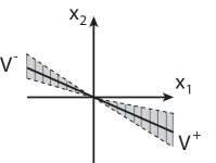
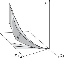
Figure 8: On the left: Projection into the $(x_{1},x_{2})$-plane of the two sets $V^{\pm}$ that are bissected by the solid line $F_{2}x_{1}+F_{3}x_{2}=0$ and are covered by the lines $x_{1}=$constant, shown here in the case $0<F_{2}/F_{3}<1$. Right: the set $V^{+}$ and its projection. Only the lighter strip is mapped back into $V^{+}$ by ${\bf g}$.

To investigate how ${\bf x}\in W_{c_{0}}$ are mapped by ${\bf g}$, we decompose $W_{c_{0}}=W^{+}\cup W^{-}$ where $W^{i}=\{(x_{1},x_{2},x_{3})\in W_{c_{0}}:~{}ix_{1}>0\}$ and

$$W^{+}=\bigcup_{\stackrel{{\scriptstyle-\beta_{2}/(\beta_{1}+\beta_{2}^{2})<r<-1/\beta_{2}}}{{x_{1}<\delta}}}V^{+}(x_{1},-c_{0},c_{0},r),\qquad W^{-}=\bigcup_{\stackrel{{\scriptstyle-\beta_{2}/(\beta_{1}+\beta_{2}^{2})<r<-1/\beta_{2}}}{{-x_{1}<\delta}}}V^{-}(x_{1},c_{0},-c_{0},r),$$

where

$$\begin{array}[]{l}V^{+}(x_{1},c_{1},c_{2},r)=\{(x_{1},x_{2},x_{1}^{r})~{}:~{}c_{1}x_{1}<|F_{2}x_{1}+F_{3}x_{2}|<c_{2}x_{1},~{}x_{1}>0\},\\ V^{-}(x_{1},c_{1},c_{2},r)=\{(x_{1},x_{2},x_{1}^{r})~{}:~{}c_{1}x_{1}<|F_{2}x_{1}+F_{3}x_{2}|<c_{2}x_{1},~{}x_{1}<0\}.\end{array}$$ (41)

We have:

$${\bf g}(x_{1},x_{2},x_{1}^{r})=(F_{1}x_{1}^{r\beta_{1}},(F_{2}x_{1}+F_{3}x_{2})x_{1}^{r\beta_{2}},(F_{4}x_{1}+F_{5}x_{2})x_{1}^{r\beta_{2}}).$$

For fixed $x_{1}$ and $r$, look at the curve $x_{2}\mapsto(x_{1},x_{2},x_{1}^{r})$ inside $W^{+}$. We claim that only a small part of this curve is mapped by ${\bf g}$ into $W_{c_{0}}$. The set ${\bf g}V^{+}(x_{1},-c_{0},c_{0},r)\cap W_{c_{0}}$ satisfies

$$-c_{0}F_{1}x_{1}^{r\beta_{1}}<F_{2}F_{1}x_{1}^{r\beta_{1}}+F_{3}(F_{2}x_{1}+F_{3}x_{2})x_{1}^{r\beta_{2}}<c_{0}F_{1}x_{1}^{r\beta_{1}},$$

which implies that the points that remain in $W_{c_{0}}$ are

$${\bf g}^{-1}({\bf g}(V^{+}(x_{1},-c_{0},c_{0},r))\cap W_{c_{0}})=V^{+}(x_{1},c^{\prime}-\tilde{c},c^{\prime}+\tilde{c},r),$$ (42)

where

$$c^{\prime}=-\frac{F_{1}F_{2}}{F_{3}}x_{1}^{\beta_{1}r-\beta_{2}r-1},\quad\tilde{c}=-\frac{c_{0}F_{1}}{F_{3}}x_{1}^{\beta_{1}r-\beta_{2}r-1}.$$ (43)

(Note, that $r>-\beta_{2}/(\beta_{1}+\beta_{2}^{2})$ implies that $\beta_{1}r-\beta_{2}r-1>\beta_{1}(-\beta_{2}-1)/(\beta_{1}+\beta_{2}^{2})>0$.) Moreover, for asymptotically small $x_{1}$ we can write

$${\bf g}(V^{+}(x_{1},-c_{0},c_{0},r))\cap W_{c_{0}}\approx V^{+}(F_{1}x_{1}^{r\beta_{1}},-c_{0},c_{0},r^{\prime}),\hbox{ where }r^{\prime}=(1+\beta_{2}r)/(r\beta_{1}).$$ (44)

Here $r^{\prime}>0$ because $r<-1/\beta_{2}$. Similar estimates holds true for $V^{-}(x_{1},c_{0},-c_{0},r)$.

We represent each one of the sets $W^{+}$ and $W^{-}$ as the union of a $(x_{1},r)$-familiy of curves parametrised by $x_{2}$. From (42) and (43) we obtain that

$$\frac{l_{1}({\bf g}^{-1}({\bf g}V^{+}(x_{1},-c_{0},c_{0},r)\cap W_{c_{0}}))}{l_{1}(V^{+}(x_{1},-c_{0},c_{0},r)))}=\frac{\tilde{c}}{c_{0}}<Cx_{1}^{\beta_{1}r-\beta_{2}r-1},$$ (45)

where $l_{1}$ denotes the 1-dimensional Lebesgue measure and $C$ is a constant that depends on $F_{j}$ and $\beta_{i}$. Hence, for sufficiently small $\delta$ the inclusions (40) and the estimate (44) imply that as $n\to\infty$ almost all points, except for a set of zero measure, are mapped by ${\bf g}^{n}$ away from $V_{\delta}$. Therefore, the point ${\bf x}=0$ is a completely unstable point of the map ${\bf g}$. ∎

Lemma A.4.

Consider the map ${\bf g}$ (36) where $\beta_{1}>0$, $\beta_{1}-\beta_{2}>1$ and $-1<\beta_{2}<0$. The origin is completely unstable fixed point of the map ${\bf g}$ (36).

Proof.

The proof of this lemma, and also of the two following, employs the same ideas as the proof of Lemma A.3. Namely, we decompose ${\mathbb{R}}^{3}_{\delta}$ as a union of several subsets and consider how the subsets are mapped by ${\bf g}$. We represent ${\mathbb{R}}^{3}_{\delta}=U^{I}\cup U^{II}$ and $U^{I}=U^{I}_{c_{0}}\cup W_{c_{0}}$, where

$$\begin{array}[]{l}U^{I}=\{(x_{1},x_{2},x_{3})~{}:~{}\max\{p,q\}<{\delta}\hbox{ and }p>q^{\beta_{1}-\beta_{2}-s}\},\\ U^{II}=\{(x_{1},x_{2},x_{3})~{}:~{}\max\{p,q\}<{\delta}\hbox{ and }p<q^{\beta_{1}-\beta_{2}-s}\},\\ U^{I}_{c_{0}}=\{(x_{1},x_{2},x_{3})\in U^{I}~{}:~{}|F_{2}x_{1}+F_{3}x_{2}|>c_{0}|x_{1}|\},\ W_{c_{0}}=U^{I}\setminus U^{I}_{c_{0}},\end{array}$$ (46)

$0<s<\beta_{1}$, $\beta_{1}-\beta_{2}-s>\beta_{1}/(\beta_{1}-s)$ and $0<c_{0}<\min\{1,F_{2}\}/2$.

For sufficiently small $\delta$ we have:

$$({\bf g}(U^{I}_{c_{0}})\cap V_{\delta})\subset U^{I}_{c_{0}};\qquad({\bf g}(U^{II})\cap V_{\delta})\subset U^{I}.$$ (47)

The latter inclusion holds true due to our choice of $s$.

For any ${\bf x}\in U^{I}_{c_{0}}$ for small $\delta$ we have $g_{1}({\bf x})\ll g_{2}({\bf x})$, hence for $n>2$ we can write

$${\bf g}^{n}({\bf x})\approx(F_{1}({\bf g}^{n-1}_{3}({\bf x}))^{\beta_{1}},F_{3}{\bf g}^{n-1}_{2}({\bf g}^{n-1}_{3}({\bf x}))^{\beta_{2}},F_{5}{\bf g}^{n-1}_{2}({\bf g}^{n-1}_{3}({\bf x}))^{\beta_{2}}).$$

Therefore,

$${\bf g}^{n+1}({\bf x})\approx(F_{1}({\bf g}^{n}_{3}({\bf x}))^{\beta_{1}},F_{3}^{\prime}({\bf g}^{n}_{3}({\bf x}))^{1+\beta_{2}},F_{5}^{\prime}({\bf g}^{n}_{3}({\bf x}))^{1+\beta_{2}}).$$

which implies that for any ${\bf x}\in U^{I}_{c_{0}}$ we have ${\bf g}^{n}({\bf x})\not\in V_{\delta}$ for large $n$.

We decompose further:

$$W_{c_{0}}=\cup_{\pm}\bigcup_{x_{1}<\delta,~{}-1/(\beta_{1}-\beta_{2}-s)<r<\infty}V^{\pm}(x_{1},\mp c_{0},\pm c_{0},r),$$ (48)

where $V^{\pm}(x_{1},c_{1},c_{2},r)$ are defined by (41).

The set $V^{+}$ is mapped as ${\bf g}(V^{+})\subset U^{I}_{c_{0}}\cup W_{c_{0}}\cup U^{II}$. We have accounted for points that go to $U^{I}_{c_{0}}$. Below, we first show that the set of points that are mapped to $W_{c_{0}}$ is small. Then, for points mapped to $U^{II}$ we will have to consider a second iteration of ${\bf g}$ to show that the set of points that are first mapped to $U^{II}$ and then to $W_{c_{0}}$ is small. (The points that are first mapped to $U^{II}$ and then to $U^{I}_{c_{0}}$ are already accounted for. ) As in the proof of the previous lemma, this implies that when the number of iterations goes to infinity almost all points are mapped to $U^{I}_{c_{0}}$, and then away from $V_{\delta}$.

We have (see the proof of Lemma A.3)

$${\bf g}^{-1}({\bf g}(V^{+}(x_{1},-c_{0},c_{0},r))\cap W_{c_{0}})=V^{+}(x_{1},c^{\prime}-\tilde{c},c^{\prime}+\tilde{c},r),$$ (49)

where $\tilde{c}=c_{0}F_{1}x_{1}^{\beta_{1}r-\beta_{2}r-1}/F_{3}$. Since $\beta_{1}r-\beta_{2}r-1>s/(\beta_{1}-\beta_{2}-s)>0$, we estimate

$$\frac{l_{1}({\bf g}^{-1}({\bf g}(V^{+}(x_{1},-c_{0},c_{0},r))\cap W_{c_{0}}))}{l_{1}(V^{+}(x_{1},-c_{0},c_{0},r)))}=\frac{\tilde{c}}{c_{0}}<Cx_{1}^{s/(\beta_{1}-\beta_{2}-s)}.$$ (50)

Next, we consider ${\bf g}({\bf g}(V^{+}(x_{1},-c_{0},c_{0},r))\cap U^{II})$. For ${\bf x}=(x_{1},-F_{2}x_{1}/F_{3}+cx_{1},x_{1}^{r})$ we have

$${\bf g}^{2}({\bf x})=(\tilde{F}_{1}x_{1}^{\beta_{1}(1+r\beta_{2})},(\tilde{F}_{2}x_{1}^{\beta_{1}r}+c\tilde{F}_{3}x_{1}^{1+r\beta_{2}})x_{1}^{\beta_{2}(1+r\beta_{2})},(\tilde{F}_{4}x_{1}^{\beta_{1}r}+c\tilde{F}_{5}x_{1}^{1+r\beta_{2}})x_{1}^{\beta_{2}(1+r\beta_{2})}).$$

Therefore,

$${\bf g}^{-2}({\bf g}({\bf g}(V^{+}(x_{1},-c_{0},c_{0},r))\cap U^{II})\cap W_{c_{0}})=V^{+}(x_{1},c^{*}-\hat{c},c^{*}-\hat{c},r),$$ (51)

where $\hat{c}=\hat{C}x_{1}^{(1+r\beta_{2})(\beta_{1}-\beta_{2}-1)}$. Moreover,

$${\bf g}({\bf g}(V^{+}(x_{1},-c_{0},c_{0},r))\cap U^{II})\cap W_{c_{0}}\subset V^{+}(x_{1},-c_{0},c_{0},r^{\prime}),$$ (52)

where $r^{\prime}=(\min\{r\beta_{1},1+r\beta_{2}\}+\beta_{2})/\beta_{1}$. Therefore, due to (47)-(52) for sufficiently small $\delta$, almost all ${\bf x}\in V_{\delta}$ satisfy $|{\bf g}^{n}({\bf x})|>\delta$ as $n\to\infty$. ∎

Lemma A.5.

Consider the map ${\bf g}$ (36) where $\beta_{1}>0$, $\beta_{1}-\beta_{2}<1$ and $-1<\beta_{2}<0$. The origin is completely unstable fixed point of the map ${\bf g}$ (36).

Proof.

We decompose ${\mathbb{R}}^{3}_{\delta}=U^{I}\cup U^{II}\cup U^{III}$ and $U^{I}=U^{I}_{c_{0}}\cup W_{c_{0}}$, where

$$\begin{array}[]{l}U^{I}=\{(x_{1},x_{2},x_{3})~{}:~{}\max\{p,q\}<\delta\hbox{ and }p>q^{\beta_{1}-\beta_{2}-s_{1}}\},\\ U^{II}=\{(x_{1},x_{2},x_{3})~{}:~{}\max\{p,q\}<\delta\hbox{ and }p<q^{1-s_{2}}\},\\ U^{III}=\{(x_{1},x_{2},x_{3})~{}:~{}\max\{p,q\}<\delta\hbox{ and }q^{1-s_{2}}<p<q^{\beta_{1}-\beta_{2}-s_{1}}\},\\ U^{I}_{c_{0}}=\{(x_{1},x_{2},x_{3})\in U^{I}~{}:~{}|F_{4}x_{1}+F_{5}x_{2}|>c_{0}|x_{1}|\},\ W_{c_{0}}=U^{I}\setminus U^{I}_{c_{0}},\end{array}$$ (53)

$0<s_{1}<\min\{1,\beta_{1}\beta_{2}(\beta_{1}-\beta_{2}-1)/(\beta_{1}-\beta_{2}(\beta_{1}-\beta_{2}))\}$, $0<s_{2}<\min\{1,\beta_{2}(\beta_{1}-\beta_{2}-1)/(\beta_{1}-\beta_{2})\}$ and $c_{0}<\min\{1,F_{4}\}/2$.

Due to our choice of $s_{1}$, $s_{2}$ and $c_{0}$, for sufficiently small $\delta$ the subsets are mapped by ${\bf g}$ as follows:

$$\left({\bf g}(U^{I}_{c_{0}})\cap V_{\delta}\right)\subset U^{II};\qquad\left({\bf g}(U^{II})\cap V_{\delta}\right)\subset U^{I}_{c_{0}}.$$ (54)

Consider ${\bf x}\in U^{I}_{c_{0}}\cup U^{II}$. Due to (54), we can assume that ${\bf x}\in U^{II}$. Denote $p_{n}=\max\{|({\bf g}^{n}({\bf x}))_{1}|,|({\bf g}^{n}({\bf x}))_{2}|\}$ and $q_{n}=|({\bf g}^{n}({\bf x}))_{3}|$. For $n\to\infty$ the iterates ${\bf g}^{n}({\bf x})$ as long as ${\bf g}^{n}({\bf x})\in V_{\delta}$ satisfy
for even $n$: $(p_{n},q_{n})\approx(F_{1}^{\prime}q_{n-1}^{\beta_{1}},F_{2}^{\prime}p_{n-1}q_{n-1}^{\beta_{1}})$;
for odd $n$: $(p_{n},q_{n})\approx(F_{3}^{\prime}p_{n-1}q_{n-1}^{\beta_{1}},F_{4}^{\prime}p_{n-1}q_{n-1}^{\beta_{1}})$.
Which implies that

$$p_{n}\approx F_{5}^{\prime}q_{n}\quad\hbox{ and }\quad q_{n}\approx F_{6}^{\prime}q_{n-2}^{\beta_{1}+\beta_{2}(1+\beta_{2})}.$$

By assumption, $\beta_{1}>0$ and $\beta_{1}-\beta_{2}<1$, which implies that $\beta_{1}+\beta_{2}(1+\beta_{2})<1$, hence the iterates ${\bf g}^{n}({\bf x})$ satisfy $|{\bf g}^{n}({\bf x})|>\delta$ as $n\to\infty$.

On the other hand, for sufficiently small ${\bf x}\in U^{III}$ the map ${\bf g}$ can be approximated by ${\bf h}(p,q)=(F_{1}^{\prime}q^{\beta_{1}},F_{2}^{\prime}pq^{\beta_{2}})$. Therefore, arguments similar to the ones employed in the proof of Lemma 3.9 imply that for almost all ${\bf x}$ the iterates ${\bf g}^{n}({\bf x})$ escape from $U^{III}$ as $n\to\infty$. The iterates satisfy:

$$\hbox{if }{\bf x}\in U^{III}\hbox{ and }{\bf g}({\bf x})\in U^{III}\hbox{ then }{\bf g}^{2}({\bf x})\not\in W_{c_{0}}.$$ (55)

By decomposing $W_{c_{0}}$ similarly to (48), proceeding as in Lemma A.4 by considering ${\bf g}({\bf x})$ and ${\bf g}^{2}({\bf x})$ for ${\bf x}\in W_{c_{0}}$ and taking into account the above inclusions, we obtain that almost all points in $V_{\delta}$ either escape from $V_{\delta}$ or are mapped by ${\bf g}^{2}$ to $U^{I}_{c_{0}}\cup U^{II}$, from where they escape from $V_{\delta}$. ∎

Lemma A.6.

Consider the map ${\bf g}$ (36) where $\beta_{1}>0$, $\beta_{2}>0$ and $\beta_{1}+\beta_{2}<1$. The origin is completely unstable fixed point of the map ${\bf g}$ (36).

Proof.

We decompose ${\mathbb{R}}^{3}_{\delta}=U^{I}\cup U^{II}\cup U^{III}$, $U^{I}_{c_{0}}\subset U^{I}$, $U^{III}_{c_{0}}\subset U^{III}$ and $W_{c_{0}}=(U^{I}\cup U^{III})\setminus(U^{I}_{c_{0}}\cup U^{III}_{c_{0}})$, where

$$\begin{array}[]{l}U^{I}=\{(x_{1},x_{2},x_{3})~{}:~{}\max\{p,q\}<\delta\hbox{ and }p>q^{\beta_{1}-\beta_{2}-s_{1}}\},\\ U^{II}=\{(x_{1},x_{2},x_{3})~{}:~{}\max\{p,q\}<\delta\hbox{ and }p<q^{1+s_{2}}\},\\ U^{III}=\{(x_{1},x_{2},x_{3})~{}:~{}\max\{p,q\}<\delta\hbox{ and }q^{1+s_{2}}<p<q^{\beta_{1}-\beta_{2}-s_{1}}\},\\ U^{I}_{c_{0}}=\{(x_{1},x_{2},x_{3})\in U^{I}~{}:~{}|F_{4}x_{1}+F_{5}x_{2}|>c_{0}|x_{1}|\},\\ U^{III}_{c_{0}}=\{(x_{1},x_{2},x_{3})\in U^{III}~{}:~{}|F_{4}x_{1}+F_{5}x_{2}|>c_{0}|x_{1}|\},\end{array}$$ (56)

with $0<s_{1}<\min\{1,\beta_{2}(1-\beta_{1}+\beta_{2})/(1+\beta_{2}))\}$, $0<s_{2}<\min\{1,\beta_{2}(1-\beta_{1}+\beta_{2})/(\beta_{1}-\beta_{2})\}$ and $c_{0}<\min\{1,F_{4}\}/2$.

For sufficiently small $\delta$ we have:

$$\left({\bf g}(U^{III}_{c_{0}}\ )capV_{\delta}\right)\subset U^{III}_{c_{0}};\qquad\left({\bf g}(U^{I}_{c_{0}})\cap V_{\delta}\right)\subset U^{III}_{c_{0}};\qquad\left({\bf g}(U^{II})\cap V_{\delta}\right)\subset U^{I}_{c_{0}}.$$ (57)

By decomposing $W_{c_{0}}$ similarly to (48) and considering ${\bf g}({\bf x})$ and ${\bf g}^{2}({\bf x}$) for ${\bf x}\in W_{c_{0}}$, we prove that all points in $V_{\delta}$ are either mapped by ${\bf g}^{2}$ to $U^{III}_{c_{0}}$, or they escape from $V_{\delta}$. For ${\bf x}\in U^{III}_{c_{0}}$ we note that the map ${\bf g}({\bf x})$ can be approximated by ${\bf h}(p,q)=(F_{1}^{\prime}q^{\beta_{1}},F_{2}^{\prime}pq^{\beta_{2}})$, which implies that the iterates ${\bf g}^{n}({\bf x})$ satisfy $|{\bf g}^{n}({\bf x})|>\delta$ as $n\to\infty$. ∎

Appendix B Eigenspaces and eigenvalues near single-mode steady states

In this appendix we provide data on the network that are used in the calculations.

$$\begin{array}[]{l}{\bf e}_{11}=(1,0,0;0,0,0)/\sqrt{2},\ {\bf e}_{12}=(0,1,1;0,0,0)/\sqrt{2},\ {\bf e}_{13}=(0,1,-1;0,0,0)/\sqrt{2},\\ {\bf e}_{14}=(0,0,0;1,0,0),\ {\bf e}_{15}=(0,0,0;0,1,1)/\sqrt{2},\ {\bf e}_{16}=(0,0,0;0,1,-1)/\sqrt{2}\\ \hline\cr{\bf e}_{21}=(1,0,0;0,0,0),\ {\bf e}_{22}=(0,1,1;0,0,0)/\sqrt{2},\ {\bf e}_{23}=(0,1,-1;0,0,0)/\sqrt{2}\\ {\bf e}_{24}=(0,0,0;1,0,0),\ {\bf e}_{25}=(0,0,0;0,1,1)/\sqrt{2},\ {\bf e}_{26}=(0,0,0;0,1,-1)/\sqrt{2}\\ \hline\cr{\bf e}_{31}=(1,0,0;0,0,0),\ {\bf e}_{32}=(0,1,0;0,0,0),\ {\bf e}_{33}=(0,0,1;0,0,0),\\ {\bf e}_{34}=(0,0,0;1,0,0),\ {\bf e}_{35}=(0,0,0;0,1,0),\ {\bf e}_{36}=(0,0,0;0,0,1)\\ \tilde{\bf e}_{31}=(1,0,0;0,0,0),\ \tilde{\bf e}_{32}=(0,1,1;0,0,0)/\sqrt{2},\ \tilde{\bf e}_{33}=(0,1,-1;0,0,0)/\sqrt{2}\\ \tilde{\bf e}_{34}=(0,0,0;1,0,0),\ \tilde{\bf e}_{35}=(0,0,0;0,1,1)/\sqrt{2},\ \tilde{\bf e}_{36}=(0,0,0;0,1,-1)/\sqrt{2}\\ \hat{\bf e}_{31}=(0,1,0;0,0,0),\ \hat{\bf e}_{32}=(0,0,1;0,0,0),\ \hat{\bf e}_{33}=(1,0,0;0,0,0)\\ \hat{\bf e}_{34}=(0,0,0;0,1,0),\ \hat{\bf e}_{35}=(0,0,0;0,0,1),\ \hat{\bf e}_{36}=(0,0,0;1,0,0)\\ \hline\cr{\bf e}_{41}=(1,0,0;0,0,0),\ {\bf e}_{42}=(0,1,1;0,0,0)/\sqrt{2},\ {\bf e}_{43}=(0,1,-1;0,0,0)/\sqrt{2}\\ {\bf e}_{44}=(0,0,0;1,0,0),\ {\bf e}_{45}=(0,0,0;0,1,1)/\sqrt{2},\ {\bf e}_{46}=(0,0,0;0,1,-1)/\sqrt{2}\\ \hline\cr{\bf e}_{51}=(1,0,0;0,0,0)/\sqrt{2},\ {\bf e}_{52}=(0,1,1;0,0,0)/\sqrt{2},\ {\bf e}_{53}=(0,1,-1;0,0,0)/\sqrt{2},\\ {\bf e}_{54}=(0,0,0;1,0,0),\ {\bf e}_{55}=(0,0,0;0,1,1)/\sqrt{2},\ {\bf e}_{56}=(0,0,0;0,1,-1)/\sqrt{2}\\ \end{array}$$

Table 1: Local bases at the equilibria $\xi_{j}$.

$$\begin{array}[]{ccccc}j&\xi_{j}&{\mathbb{R}}^{6}\ominus L_{j}&\Delta_{j}&\mbox{Isotypic components}\\ \hline\cr 1&R_{z}&(0,x_{2},x_{3};y_{1},y_{2},y_{3})&<s_{1},r\gamma^{1}_{\pi/2},\gamma^{3}_{\alpha}>&(0,x_{2},x_{3};0,0,0),\ (0,0,0;y_{1},0,0)\\ &&&&(0,0,0;0,y_{2},y_{2}),\ (0,0,0;0,y_{2},-y_{2})\\ \hline\cr 2&\rho^{2}PQ_{w}&(x_{1},x_{2},x_{3};y_{1},y_{2},-y_{2})&<s_{1},r\gamma^{1}_{\pi/2},\gamma^{2}_{\pi}>&(x_{1},0,0;0,0,0),\ (0,x_{2},x_{3};0,0,0)\\ &&&&(0,0,0;y_{1},0,0),\ (0,0,0;0,y_{2},-y_{2})\\ \hline\cr 3&R_{w}&(x_{1},x_{2},x_{3};0,y_{2},y_{3})&<s_{1},\gamma^{1}_{\alpha},r\gamma^{2}_{\pi/2}>&(x_{1},0,0;0,0,0),\ (0,x_{2},x_{3};0,0,0),\\ &&&&(0,0,0;0,y_{2},y_{3})\\ {}\hfil&\rho R_{w}&(x_{1},x_{2},x_{3};y_{1},y_{2},0)&\rho<s_{1},\gamma^{1}_{\alpha},r\gamma^{2}_{\pi/2}>\rho^{2}&(x_{1},0,0;0,0,0),\ (0,x_{2},x_{3};0,0,0),\\ &&&&(0,0,0;y_{1},y_{2},0)\\ \hline\cr 4&\rho^{2}{\widetilde{PQ}}_{w}&(x_{1},x_{2},x_{3};y_{1},y_{2},y_{2})&<rs_{1},r\gamma^{1}_{\pi/4},\gamma^{2}_{\pi/2}>&(x_{1},0,0;0,0,0),\ (0,x_{2},x_{3};0,0,0),\\ &&&&(0,0,0;y_{1},0,0),\ (0,0,0;0,y_{2},y_{2})\\ \hline\cr 5&\rho^{2}PQ_{z}&(x_{1},x_{2},-x_{2};y_{1},y_{2},y_{3})&<s_{1},r\gamma^{3}_{\pi/3}>&(x_{1},0,0;0,0,0),\ (0,x_{2},-x_{2};0,0,0),\\ &&&&(0,0,0;y_{1},y_{2},y_{2}),\ (0,0,0;0,y_{2},-y_{2})\\ \end{array}$$

Table 2: Isotypic decompositions of ${\mathbb{R}}^{6}\ominus L_{j}$ under $\Delta_{j}$.

$$\begin{array}[]{cccc}\xi_{i}\to\xi_{j}&{\mathbb{R}}^{6}\ominus P_{ij}&\Sigma_{ij}&\mbox{Isotypic components}\\ \hline\cr\xi_{1}\to\xi_{2}&(0,x_{2},x_{3};y_{1},y_{2},-y_{2})&<s_{1},r\gamma^{1}_{\pi/2},\gamma^{3}_{\pi}>&(0,x_{2},x_{2};0,0,0),\ (0,x_{2},-x_{2};0,0,0)\\ &&&(0,0,0;y_{1},0,0),\ (0,0,0;0,y_{2},-y_{2})\\ \hline\cr\xi_{2}\to\rho\xi_{3}&(x_{1},x_{2},x_{3};y_{1},0,0)&<r\gamma^{1}_{\pi/2},r\gamma^{3}_{\pi/2}>&(x_{1},0,0;0,0,0),\ (0,x_{2},x_{3};0,0,0),\\ &&&(0,0,0;y_{1},0,0)\\ \hline\cr\xi_{3}\to\xi_{1}&(0,x_{2},x_{3};0,y_{2},y_{3})&<s_{1},\gamma^{1}_{\pi},\gamma^{3}_{\pi/2}>&(0,x_{2},x_{2};0,0,0),\ (0,x_{2},-x_{2};0,0,0)\\ &&&(0,0,0;0,y_{2},y_{2}),\ (0,0,0;0,y_{2},-y_{2})\\ \hline\cr\xi_{1}\to\xi_{4}&(0,x_{2},x_{3};y_{1},y_{2},y_{2})&<r\gamma^{1}_{\pi/2},s_{1}\gamma^{3}_{\pi/2}>&(0,x_{2},x_{3};0,0,0),\ (0,0,0;y_{1},0,0),\\ &&&(0,0,0;0,y_{2},y_{2})\\ \hline\cr\xi_{4}\to\xi_{5}&(x_{1},x_{2},-x_{2};y_{1},y_{2},y_{2})&<s_{1}r\gamma^{1}_{\pi},s_{1}r\gamma^{3}_{\pi}>&(x_{1},0,0;0,0,0),\ (0,x_{2},-x_{2};y_{1},y_{2},y_{2})\\ \hline\cr\xi_{5}\to\rho\xi_{1}&(x_{1},0,0;y_{1},y_{2},y_{3})&<r\gamma^{3}_{\pi/3}>&(x_{1},0,0;0,0,0),\ (0,0,0;y_{1},y_{2},y_{3})\\ \hline\cr\end{array}$$

Table 3: Isotypic decompositions of ${\mathbb{R}}^{6}\ominus P_{ij}$ under $\Sigma_{ij}$. The plane $P_{43}$ coincides with $P_{23}$, therefore it is not listed.

$$\begin{array}[]{ccccc}\mbox{Name}&\mbox{Subspace}&\mbox{Eigenvectors}&\mbox{Eigenvalues}&\mbox{Eigenvalues}\\ \hline\cr R_{z}=\xi_{1}&(q,0,0;0,0,0)&{\bf e}_{11}&\lambda_{11}\mbox{ (radial)}&2A_{1}x^{2}\\ &(0,u_{2},u_{3};0,0,0)&{\bf e}_{12},{\bf e}_{13}&\lambda_{12}=\lambda_{13}&(A_{2}-A_{1})x^{2}\\ &(0,0,0;u,0,0)&{\bf e}_{14}&\lambda_{14}&\lambda_{2}+C_{4}x^{2}\\ &(0,0,0;0,u,u)&{\bf e}_{15}&\lambda_{15}&\lambda_{2}+(C_{5}+C_{6})x^{2}\\ &(0,0,0;0,u,-u)&{\bf e}_{16}&\lambda_{16}&\lambda_{2}+(C_{5}-C_{6})x^{2}\\ \hline\cr\rho^{2}PQ_{z}=\xi_{5}&(q,0,0;0,0,0)&{\bf e}_{51}&\lambda_{51}&(A_{2}-A_{1})x^{2}\\ &(0,q,q;0,0,0)&{\bf e}_{52}&\lambda_{52}\mbox{ (radial)}&2(A_{1}+A_{2})x^{2}\\ &(0,q,-q;0,0,0)&{\bf e}_{53}&\lambda_{53}&2(A_{1}-A_{2})x^{2}\\ &(0,0,0;u_{1},u_{2},u_{2})&{\bf e}_{54},{\bf e}_{55}&\lambda_{54},\lambda_{55}&\mu_{1}+\mu_{2}=2\lambda_{2}+(C_{4}+3C_{5})x^{2}\\ &&&&\mu_{1}\mu_{2}=(\lambda_{2}+(C_{4}+C_{5})x^{2})\times\\ &&&&(\lambda_{2}+2C_{5}x^{2})-2C_{6}^{2}x^{4}\\ &(0,0,0;0,u_{2},-u_{2})&{\bf e}_{56}&\lambda_{56}&\lambda_{2}+(C_{4}+C_{5})x^{2}\\ \hline\cr R_{w}=\xi_{3}&(0,0,0;q,0,0)&{\bf e}_{34}&\lambda_{34}\mbox{ (radial)}&2B_{1}y^{2}\\ &(0,0,0;0,u_{2},u_{3})&{\bf e}_{35},{\bf e}_{36}&\lambda_{35},\lambda_{36}&(B_{2}-B_{1})y^{2}\\ &(u,0,0;0,0,0)&{\bf e}_{31}&\lambda_{31}&\lambda_{1}+C_{1}y^{2}\\ &(0,u_{2},u_{3};0,0,0)&{\bf e}_{32},{\bf e}_{33}&\lambda_{32}=\lambda_{33}&\lambda_{1}+C_{2}y^{2}\\ \hline\cr\rho R_{w}=\rho\xi_{3}&(0,0,0;0,q,0)&{\bf e}_{34}&\lambda_{34}\mbox{ (radial)}&2B_{1}y^{2}\\ &(0,0,0;u_{1},u_{2},0)&{\bf e}_{35},{\bf e}_{36}&\lambda_{35},\lambda_{36}&(B_{2}-B_{1})y^{2}\\ &(0,u,0;0,0,0)&{\bf e}_{31}&\lambda_{31}&\lambda_{1}+C_{1}y^{2}\\ &(u_{1},u_{2},0;0,0,0)&{\bf e}_{32},{\bf e}_{33}&\lambda_{32}=\lambda_{33}&\lambda_{1}+C_{2}y^{2}\\ \hline\cr\rho^{2}PQ_{w}=\xi_{2}&(0,0,0;u,0,0)&{\bf e}_{24}&\lambda_{24}&(B_{2}-B_{1})y^{2}\\ &(0,0,0;0,q,q)&{\bf e}_{25}&\lambda_{25}\mbox{ (radial)}&2(B_{1}+B_{2})y^{2}\\ &(0,0,0;0,q,-q)&{\bf e}_{26}&\lambda_{26}&2(B_{1}-B_{2})y^{2}\\ &(q,0,0;0,0,0)&{\bf e}_{21}&\lambda_{21}&\lambda_{1}+(2C_{2}+C_{3})y^{2}\\ &(0,u_{2},u_{3};0,0,0)&{\bf e}_{22},{\bf e}_{23}&\lambda_{22}=\lambda_{23}&\lambda_{1}+(C_{1}+C_{2})y^{2}\\ \hline\cr\rho^{2}{\widetilde{PQ}}_{w}=\xi_{4}&(0,0,0;0,q,q)&{\bf e}_{45}&\lambda_{45}&2(B_{1}-B_{2})y^{2}\\ &(0,0,0;0,q,-q)&{\bf e}_{46}&\lambda_{46}\mbox{ (radial)}&2(B_{1}+B_{2})y^{2}\\ &(q,0,0;0,0,0)&{\bf e}_{41}&\lambda_{41}&\lambda_{1}+(2C_{2}-C_{3})y^{2}\\ &(0,u_{1},u_{2};0,0,0)&{\bf e}_{42},{\bf e}_{43}&\lambda_{42}=\lambda_{43}&\lambda_{1}+(C_{1}+C_{2})y^{2}\\ &(0,0,0;q,0,0)&{\bf e}_{44}&\lambda_{44}&(B_{2}-B_{1})y^{2}\end{array}$$

Table 4: Eigenspaces and associated eigenvalues near equilibria in the network.

References

- [1] M.A.D. Aguiar and S.B.S.D. Castro. Chaotic switching in a two-person game. Physica D: Nonlinear Phenomena 239–16, 1598–1609 (2010).
- [2] P. Ashwin and C. Postlethwaite. On designing heteroclinic networks from graphs, Phys. D. 265, 26–39 (2013).
- [3] S.B.S.D. Castro, I.S. Labouriau and O. Podvigina. A heteroclinic network in mode interaction with symmetry, Dynamical Systems 25, (2010)
- [4] S.B.S.D. Castro and A. Lohse. Stability in simple heteroclinic networks in , Dynamical Systems 29 (4), 451–481 (2014)
- [5] M.J. Field. Heteroclinic networks in homogeneous and heterogeneous identical cell systems, J. Nonlinear Sci. 25, 779–813 (2015).
- [6] L. Garrido-da-Silva and S.B.S.D. Castro. Stability of quasi-simple heteroclinic cycles, Dynamical Systems, to appear
- [7] M. Golubitsky, I.N Stewart and D. Schaeffer. Singularities and Groups in Bifurcation Theory. Volume 2. Appl. Math. Sci. 69, Springer-Verlag, New York, (1988).
- [8] J. Guckenheimer and P. Holmes. Structurally stable heteroclinic cycles, Math. Proc. Camb. Phil. Soc., 103, 189–192 (1988).
- [9] J. Hofbauer and K. Sigmund. Evolutionary game dynamics, Bull. Amer. Math. Soc., 40, 479–519 (2003).
- [10] V. Kirk, E. Lane, C.M. Postlethwaite, A.M. Rucklidge, and M. Silber. A mechanism for switching near a heteroclinic network, Dynamical Systems: An International Journal, 25(3), 323–349 (2010).
- [11] M. Krupa and I. Melbourne. Asymptotic Stability of Heteroclinic Cycles in Systems with Symmetry. Ergodic Theory and Dynam. Sys, 15, 121–147 (1995).
- [12] M. Krupa and I. Melbourne. Asymptotic Stability of Heteroclinic Cycles in Systems with Symmetry II, Proc. Roy. Soc. Edinburgh, 134A, 1177–1197 (2004).
- [13] A. Lohse. Stability of heteroclinic cycles in transverse bifurcations, Physica D, 310, 95–103 (2015)
- [14] I. Melbourne. An example of a non-asymptotically stable attractor, Nonlinearity 4, 835–844 (1991).
- [15] M. Mecchia, B. Zimmermann. On finite groups acting on homology 4-spheres and finite subgroups of SO(5). Top. Appl. 158, 741 – 747 arXiv:1001.3976 [math.GT] (2011).
- [16] O. Podvigina. Stability and bifurcations of heteroclinic cycles of type Z, Nonlinearity 25, 1887–1917 (2012).
- [17] O. Podvigina. Classification and stability of simple homoclinic cycles in , Nonlinearity 26, 1501–1528 (2013).
- [18] O.M. Podvigina and P.B. Ashwin. On local attraction properties and a stability index for heteroclinic connections. Nonlienarity 24, 887–929 (2011).
- [19] O. Podvigina and P. Chossat. Asymptotic Stability of Pseudo-simple Heteroclinic Cycles in , J. Nonlinear Sci., 27, 343–375 (2017).
- [20] C. Postlethwaite. A new mechanism for stability loss from a heteroclinic cycle, Dyn. Syst., 25, 305–322 (2010).
- [21] C. Postlethwaite and J.H.P. Dawes. Resonance bifurcations from robust homoclinic cycles, Nonlinearity, 23, 621–642 (2010).
- [22] G.L. dos Reis. Structural Stability of Equivariant Vector Fields on Two-Dimensions, Trans. Am. Math. Soc., 283, 633–643 (1984).
- [23] N. Sottocornola. Simple homoclinic cycles in low-dimensional spaces. J. Differential Equations 210, 135 – 154 (2005).