Identifiability of tree-child phylogenetic networks under a probabilistic recombination-mutation model of evolution

Abstract.

Phylogenetic networks are an extension of phylogenetic trees which are used to represent evolutionary histories in which reticulation events (such as recombination and hybridization) have occurred. A central question for such networks is that of identifiability, which essentially asks under what circumstances can we reliably identify the phylogenetic network that gave rise to the observed data? Recently, identifiability results have appeared for networks relative to a model of sequence evolution that generalizes the standard Markov models used for phylogenetic trees. However, these results are quite limited in terms of the complexity of the networks that are considered. In this paper, by introducing an alternative probabilistic model for evolution along a network that is based on some ground-breaking work by Thatte for pedigrees, we are able to obtain an identifiability result for a much larger class of phylogenetic networks (essentially the class of so-called tree-child networks). To prove our main theorem, we derive some new results for identifying tree-child networks combinatorially, and then adapt some techniques developed by Thatte for pedigrees to show that our combinatorial results imply identifiability in the probabilistic setting. We hope that the introduction of our new model for networks could lead to new approaches to reliably construct phylogenetic networks.

1. Introduction

Recently, there has been growing interest in the construction of phylogenetic networks in order to represent the evolutionary history of a given set of species or taxa [1]. Phylogenetic networks are a generalization of phylogenetic trees, and they have the advantage of being able to represent evolutionary events such as recombination and hybridization that is not possible within a single tree. Various approaches have been developed for constructing networks [7, 9], and more recently the use of probabilistic approaches for this purpose has started to gain momentum.

One of the key issues that arises when applying probabilistic models in phylogenetics is that of identifiability: under what circumstances can we reliably identify the phylogenetic tree or network that gave rise to the observed data? Typically, as is the case in this paper, the observed data is a multiple alignment of sequences across a set of taxa, which correspond to the leaves of the tree or network. This identifiability problem has been extensively studied for phylogenetic trees where identifiability has been proven for simple models some time ago (see e.g. [4, 13] as well as [11] for an overview of some more recent developments), but relatively little is known for more general networks.

Identifiability results for phylogenetic networks come with two riders: the model of evolution considered on the network; and the class of networks considered. Most studies use a model of evolution on a rooted binary phylogenetic network, in which characters evolve along arcs, copy themselves at tree vertices, and make a random choice at reticulation vertices [10]. Under this model of evolution, identifiability results are known for a limited set of families of networks. For instance [6] have shown that under such a model, networks with a single cycle of length greater than or equal to 4 are identifiable. Related network-based models consider evolution along the trees that are contained within a network and take into account processes such as incomplete lineage sorting [16], but identifiability of these models is complicated by the fact that the trees displayed in a network do not necessarily identify the network.

In this paper we consider a different evolutionary model, which we adapt from the world of pedigree reconstruction [15]. In this model, which we illustrate in Figure 1, first a tree is selected at random from the set of trees displayed by a network, and a standard model of evolution on that tree (see e.g. [5, Chapter 13]) is used to generate character values at sites until the tree changes. At each site and for each reticulation vertex there is a fixed (small) probability $p$ that the parent of the vertex will switch. For networks whose displayed trees have leaf-set equal to that of the network, this generates a Markov process whose state space is the set of displayed trees of the network, and means that an alignment will have blocks of sites generated under a common tree, before a change produces another block of sites generated under a new tree. Related approaches have been considered in the literature for constructing networks (known as ancestral recombination graphs) from an alignment of recombining sequences [12], and also for inferring break-points in such alignments using the so-called multiple changepoint model [14].

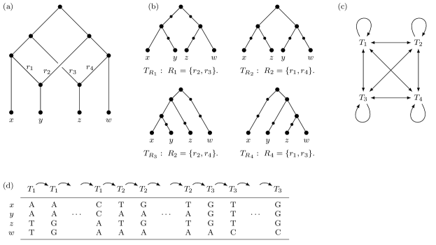
Figure 1. (a) A phylogenetic network with two reticulations and reticulation arcs labelled $r_{i}$ (Section 2.2). All arcs are directed downwards and away from the root. (b) The four rooted trees $T_{R_{i}}$ in the network corresponding to choices of sets of reticulation arcs $R_{i}$ (Section 3). (c) The Markov model on the four trees allows movement between any pair of trees by changing choice of $R_{i}$ (abbreviating $T_{R_{i}}$ to $T_{i}$). This is introduced in Section 4.1. (d) An alignment generated by the sequence of trees $T_{1}\to T_{1}\to\dots\to T_{1}\to T_{2}\to T_{2}\to\dots\to T_{2}\to T_{3}\to T_{3}\to\dots\to T_{3}$ (Section 4.1).

Under our model of evolution along a phylogenetic network, we are able to obtain an identifiability result for a much larger class of networks than has been possible before. In particular, in our main result, Corollary 6.3, we show that it is possible identify any network within the class of tree-child networks, all of which have same number of reticulation vertices, and such that none of them has a reticulation vertex adjacent to the root (see Section 1 for the definition of these terms). Whereas for the model used in [6] network identifiability has only been shown to hold for the case where there is a single reticulation, the networks that we consider can have any number of reticulations (if the number of leaves is allowed to grow).

We now summarize the rest of the paper. We begin with a section defining the key terms that will be used throughout the paper (Section 2). Section 3 provides key results on tree-child networks that we will need, some of them new. In particular we prove that the number of non-isomorphic “embedded spanning trees” in a tree-child network is 2 raised to power of the number of reticulation vertices in the network (Theorem 3.3), and that if two tree-child networks have the same set of embedded spanning trees, then they are isomorphic (Theorem 3.5). In Section 4 we introduce the model of evolution that we will study on a network, based on that of [15] for pedigrees, and we adapt the key results of [15] for the setting of rooted binary phylogenetic networks. Our main result is contained in Section 6, and it is based on a result which states that if the distributions of the characters arising on certain networks are the same then, for sufficiently long alignments and a certain choice of model parameter, the networks must contain the same set of embedded spanning trees (Corollary 6.2). This, in turn, is a direct corollary of a technical result (Theorem 6.1) whose proof employs a similar strategy to that used in the proof of [15, Theorem 2]. We conclude with a short discussion on possible future directions.

2. Preliminaries/Definitions

2.1. Trees and forests

In what follows $X$ is a finite set (corresponding to a set of taxa).

A forest is a graph with no cycles; a tree is a forest with one connected component. A leaf in a forest is a degree 1 vertex. A rooted tree is a tree with one vertex identified called the root, and all arcs directed away from the root towards the leaves. Note that if the root has out-degree 1, then we do not regard it as being a leaf of the tree.

Following [15, Definitions 4 and 6], we define an $X$-forest to be a forest with leaf-set $X$, and say that two $X$-forests $F_{1}$ and $F_{2}$ are isomorphic if there is a graph isomorphism between $F_{1}$ and $F_{2}$ which is the identity on $X$. An $X$-tree $T$ is an $X$-forest with one component such that all internal vertices of $T$ have degree either 2 or 3. Note, that $X$-forests are unrooted. Moreover, it is important to note that an $X$-forest (or $X$-tree) may contain vertices of degree 2 that are not contained in $X$, and so the term is used in a slightly different way from that commonly used in the phylogenetics literature.

2.2. Phylogenetic networks

For networks we follow the definitions presented in [2].

A phylogenetic network $N$ on $X$ is a directed acyclic graph with the following properties: (i) it has a unique vertex of in-degree zero called the root, which has out-degree two (except in the case $|X|=1$), (ii) the set $X$ labels the set of vertices of out-degree zero, each of which has in-degree one, and (iii) every other vertex either has in-degree one and out-degree two, or in-degree two and out-degree one. For technical reasons, in case $|X|=1$, then $N$ consists of the single vertex in X.

We denote the set of arcs in a phylogenetic network $N$ by $A(N)$. The vertices of out-degree zero are called leaves, while the vertices of in-degree one and out-degree two are called tree vertices and the vertices of in-degree two and out-degree one are called reticulations. The arcs directed into a reticulation are called reticulation arcs; all other arcs are called tree arcs. We let $r(N)$ denote the number of reticulations in $N$. We say that two phylogenetic networks $N_{1}$ and $N_{2}$ are isomorphic if there exists a directed graph isomorphism between $N_{1}$ and $N_{2}$ which is the identity when restricted to $X$.

For any two vertices $u$ and $v$ in $N$ that are joined by an arc $(u,v)$, we say $u$ is a parent (or parent vertex) of $v$ and, conversely, $v$ is a child (or child vertex ) of $u$. We say that $N$ is a tree-child network if every non-leaf vertex has a child which is either a tree vertex or a leaf [3].

3. Tree child networks and embedded spanning trees

Given a phylogenetic network $N$, we can obtain a rooted tree from $N$ by removing one of the two reticulation arcs incident to each one of the reticulations in $N$. If $R$ denotes a set of reticulation arcs removed in this way, then we let $T_{R}$ denote this tree. We let $\mathcal{R}_{N}$ denote the set of all possible such sets $R$ (so that $|\mathcal{R}_{N}|=2^{r(N)}$). Note that the vertex set of $T_{R}$ contains $X$ and it may potentially contain degree two vertices, as well as leaves that are not contained in $X$.

Given a network $N$, we say that a tree whose vertex set contains $X$ is an embedded spanning tree in $N$ if it is isomorphic to the (unrooted) tree which is obtained from $T_{R}$ for some $R\in\mathcal{R}_{N}$, by ignoring directions on arcs, via an isomorphism of trees which is the identity on $X$. We denote the set of all possible embedded spanning trees in $N$ (up to isomorphism) by $S(N)$. Clearly $1\leq|S(N)|\leq 2^{r(N)}$. An example is shown in Figure 2.

Figure 2. The set of embedded spanning trees $S(N)=\{S_{1},S_{2},S_{3},S_{4}\}$ for the network shown in Figure 1, and corresponding to the rooted analogues $T_{R_{1}},\dots,T_{R_{4}}$.

Later, we shall focus on tree-child networks. Note that an embedded spanning tree in a tree-child network $N$ on $X$ may not necessarily be an $X$-tree. We now characterize those tree-child networks for which every embedded spanning tree is an $X$-tree.

Lemma 3.1.

Suppose that $N$ is a tree-child network. Then every element in $S(N)$ is an $X$-tree if and only if there does not exist an arc $(\rho,v)$ in $N$ with $\rho$ the root of $N$ and $v$ a reticulation of $N$.

Proof.

Suppose that every element in $S(N)$ is an $X$-tree. Suppose $N$ contains an arc $(\rho,v)$ with $\rho$ the root of $N$ and $v$ a reticulation of $N$. If $R\in\mathcal{R}_{N}$ with $(\rho,v)\in R$, the underlying (undirected) tree of $T_{R}$ is a tree whose vertex set contains $X$ with a leaf (corresponding to $\rho$) that is not in $X$, a contradiction.

Conversely, suppose there does not exist an arc $(\rho,v)$ in $N$ with $\rho$ the root of $N$ and $v$ a reticulation of $N$. Let $R\in\mathcal{R}_{N}$, and suppose that the embedded spanning tree arising from $T_{R}$ contains a leaf $w$ that is not in $X$.

Note first that $w$ is not the root of $N$, since otherwise there would be an arc $(w,v)$ in $N$ with $v$ a reticulation of $N$, which is contradiction. So, as $w$ is not in $X$, it therefore follows that $w$ is either a reticulation or a tree-vertex. But $w$ cannot be a reticulation since then there would have to be a reticulation $v$ with $(w,v)$ an arc in $N$, which contradicts $N$ being tree-child. Similarly, $w$ cannot be a tree-vertex, as then to have $w$ being a leaf in $T_{R}$, both of the children of $w$ in $N$ would have to be reticulation vertices, which again contradicts $N$ being tree-child. This final contradiction completes the proof of the lemma. ∎

In the following we will use two operations on phylogenetic networks as defined in [2]. Let $N$ be a phylogenetic network on $X$. A 2-element subset $\{x,y\}$ of $X$ is a cherry in $N$ if the parents of $x$ and $y$ are the same. A cherry reduction on a cherry $\{x,y\}$ in $N$ is the operation of deleting $x$ and $y$, and their incident arcs, and labelling their common parent (now itself a leaf) with a new element not in $X$. Note that after a cherry reduction the number of leaves in the resulting network is reduced by one, but the number of reticulations is unchanged.

A two-element subset $\{x,y\}$ of $X$ is called a reticulated cherry in $N$ if there is an undirected path, say $x,v_{1},v_{2},y$, between $x$ and $y$ in $N$ with one of $v_{1}$ and $v_{2}$ a tree vertex and the other a reticulation vertex. A reticulated cherry reduction on a reticulated cherry $\{x,y\}$ in $N$ is the operation of deleting the reticulation arc of the reticulated cherry and suppressing the degree-two vertices resulting from the deletion. Note that after a reticulated cherry reduction, the number of reticulations in the resulting network is reduced by one, but the leaf set is unchanged.

The following result, that will be key to us, is shown in [2].

Theorem 3.2 ([2]).

If $N$ is tree-child network on $X$, then the following hold:

1. If $|X|\geq 2$, then $N$ contains either a cherry or a reticulated cherry.

2. If $N^{\prime}$ is obtained from $N$ by reducing either a cherry or a reticulated cherry, then $N^{\prime}$ is a tree-child network.

Note that using this theorem it is straight-forward to check that in case $|X|=2$, then if $X=\{x,y\}$ a tree-child network on $X$ must be isomorphic to one of the two networks in Figure 3.

Figure 3. The two tree-child networks with two leaves.

We now prove that if $N$ is tree-child then $S(N)$ must be as large as is possible for a network.

Theorem 3.3.

Suppose that $N$ is a tree-child network. Then $|S(N)|=2^{r(N)}$.

Proof.

We will show that if $R\neq R^{\prime}\in\mathcal{R}_{N}$, then the embedded spanning trees in $S(N)$ arising for $T_{R}$ and $T_{R^{\prime}}$ (which we denote by $S_{R}$ and $S_{R^{\prime}}$, respectively) are not isomorphic via an isomorphism of trees which is the identity on $X$.

Suppose this is not the case. Let $X$ be of minimal size such that there is a tree-child network $N$ on $X$ with $R\neq R^{\prime}\in\mathcal{R}_{N}$, but $S_{R}$ is isomorphic to $S_{R^{\prime}}$. Moreover, out of all such networks on $X$, pick $N$ which has a minimal number of arcs. It is straight-forward to check using the above observation for tree-child networks with two leaves that $|X|$ must be greater than $2$.

Since $N$ is tree-child, it must contain a cherry or reticulate cherry (Theorem 3.2(i)). If it contains a cherry, then perform a cherry reduction on $N$ to obtain a tree-child network $M$. This reduction does not affect any reticulation arcs, and so $R$ and $R^{\prime}$ are both subsets of the arcs of $M$. Moreover, as $S_{R}$ is isomorphic to $S_{R^{\prime}}$, this also holds for the reduced versions of $S_{R}$ and $S_{R^{\prime}}$. But this contradicts the fact that $X$ was chosen to be minimal, since $M$ has a smaller leaf-set than $N$.

If $N$ contains a reticulate cherry, then perform a reticulate cherry reduction on $N$ to obtain a tree-child network $M$ (by Theorem 3.2(ii)). Let $r$ be the reticulation arc which is removed in the reduction, and $r^{\prime}\neq r$ be the reticulation arc that is incident with $r$. Note that we must have either $r\in R\cap R^{\prime}$ or $r^{\prime}\in R\cap R^{\prime}$, or else it is straight-forward to check that $S_{R}$ is not isomorphic to $S_{R^{\prime}}$, a contradiction. So, suppose $p$ is equal to $r$ or $r^{\prime}$ and $p\in R\cap R^{\prime}$. Then as $R\neq R^{\prime}$ and $|R|=|R^{\prime}|$, $R-\{p\}$ and $R^{\prime}-\{p\}$ must both be non-empty, and $R-\{p\}\neq R^{\prime}-\{p\}$. Moreover, we can consider $R-\{p\}$ and $R^{\prime}-\{p\}$ as being contained in the set of reticulation arcs in $M$. But the reduced versions of $S_{R}$ and $S_{R^{\prime}}$ in $M$ must be isomorphic, which contradicts the choice of $N$, since $M$ has less arcs than $N$. ∎

We now show that if two tree-child networks have the same set of embedded spanning trees, then they must be isomorphic. We begin with a useful observation:

Lemma 3.4.

Suppose that $N$ and $N^{\prime}$ are tree-child networks on $X$. If, for $x,y\in X$, either of the following hold:

• $N$ contains a cherry $\{x,y\}$ and $N^{\prime}$ does not; or

• $N$ contains a reticulate cherry $\{x,y\}$ with $y$ the leaf below the reticulation and $N^{\prime}$ does not,

then $S(N)\neq S(N^{\prime})$.

Proof.

(i) Suppose $N$ contains a cherry $\{x,y\}$ and $N^{\prime}$ does not. Then in the underlying graph for $N$ there is a path of length 2 between $x$ and $y$, whereas in the underlying graph for $N^{\prime}$ there is no such path. It easily follows that $S(N)\neq S(N^{\prime})$.

(ii) Suppose $N$ contains a reticulate cherry $\{x,y\}$ with $y$ the reticulation leaf, and $N^{\prime}$ does not, but that $S(N)=S(N^{\prime})$. Note that every tree in $S(N)$ contains either

1. a path $x,u,v,y$ of length 3 between $x$ and $y$ with $v$ degree 2, or

2. two paths of length 2 of the form $x,u^{\prime},v^{\prime}$ where $u^{\prime}$ is a degree 2 vertex and $y,u^{\prime\prime},v^{\prime\prime}$ where $u^{\prime\prime}$ has degree 2, and no path between $x$ and $y$ of length less than 4,

(see Figure 4). Moreover, there exists at least one tree in $S(N)$ which contains (a) and at least one that contains (b).

Figure 4.

Since $S(N)=S(N^{\prime})$, and since they are non-empty, there must be some tree in $S(N^{\prime})$ which has a path of length 3 between $x$ and $y$. Let $x,a,b,y$ be this path. Then in the network $N^{\prime}$ it is straight-forward to check that we must have one of the following possible cases: (1) $a$ is a tree vertex and $b$ is a reticulation, (2) $b$ is a tree vertex and $a$ is a reticulation, or (3) $a$ and $b$ are both tree vertices, or (4) one of $a,b$ is a tree vertex and the other the root vertex.

First, note that (1) is not possible as then $N^{\prime}$ contains a reticulate cherry $\{x,y\}$ with $y$ the reticulation leaf. In case (2) it follows that $N^{\prime}$ contains a reticulate cherry $\{x,y\}$ with $x$ the reticulation leaf. But then there is no tree in $S(N^{\prime})$ which contains structure (a), which contradicts $S(N)=S(N^{\prime})$. In cases (3) and (4), there is no tree in $S(N^{\prime})$ which contains structure (b), again a contradiction. ∎

We are now able to prove the main result of this section, namely that sets of embedded spanning trees characterise tree-child networks.

Theorem 3.5.

Suppose that $N$ and $N^{\prime}$ are tree-child networks on $X$. Then $S(N)=S(N^{\prime})$ if and only if $N$ is isomorphic to $N^{\prime}$.

Proof.

The reverse direction is immediate: networks that are isomorphic will have the same set of embedded spanning trees. It remains to show that if $S(N)=S(N^{\prime})$ then $N$ and $N^{\prime}$ are isomorphic.

For the purposes of obtaining a contradiction, suppose that there exists a pair $N,N^{\prime}$ of non-isomorphic tree-child networks on some set $X$, with $S(N)=S(N^{\prime})$. It is straight-forward to check that $|X|>2$ using the observation made after Theorem 3.2 concerning tree-child networks with two leaves. Take $|X|$ minimal for which there exists such a pair, and out of all these pairs on $X$, take a pair which minimizes $\min\{|A(N)|,|A(N^{\prime})|\}$ (without loss of generality suppose that this minimum is obtained for $N$).

Consider the chosen minimal pair $N,N^{\prime}$. Since $N$ is tree-child, it must contain either a cherry or a reticulated cherry, by Theorem 3.2. Moreover, it follows by Lemma 3.4 that if $N$ contains a cherry $\{x,y\}$ then so must $N^{\prime}$ (otherwise $S(N)\neq S(N^{\prime})$), and that if $N$ contains a reticulate cherry $\{x,y\}$ with $y$ the reticulation leaf, then so must $N^{\prime}$.

Now, note that if $N$ and $N^{\prime}$ are not isomorphic and both have a cherry $\{x,y\}$ (respectively both have a reticulated cherry $\{x,y\}$ with $y$ the reticulation leaf), then the tree-child networks $M$ and $M^{\prime}$ obtained by performing a cherry reduction on $\{x,y\}$ for $N$ and $N^{\prime}$ (respectively a reticulated cherry reduction on $\{x,y\}$ for $N$ and $N^{\prime}$) are not isomorphic. To see this, note that if $M$ and $M^{\prime}$ are isomorphic, then we can extend the isomorphism to $N$ and $N^{\prime}$.

Putting this together, if $N$ and $N^{\prime}$ both contain a cherry $\{x,y\}$, then perform a cherry reduction on both, to obtain two necessarily non-isomorphic tree-child networks $M$ and $M^{\prime}$ with $S(M)=S(M^{\prime})$ (the last equality follows from $S(N)=S(N^{\prime})$). But this contradicts the choice of $N$ and $N^{\prime}$ since the leaf-sets of $M$ and $M^{\prime}$ are the same and this leaf-set is smaller than $X$. And, if $N$ and $N^{\prime}$ both contain a reticulate cherry $\{x,y\}$ with $y$ the leaf below the reticulation, then perform a reticulate cherry reduction on both, to obtain two necessarily non-isomorphic tree-child networks $M$ and $M^{\prime}$ with $S(M)=S(M^{\prime})$. But this again contradicts the choice of $N$ and $N^{\prime}$ since $M$ has a smaller number of arcs than $N$. ∎

4. The tree model

4.1. Evolution along a tree

We will consider the model $M=M(\mu)$, $\mu\in[0,1]$, of evolution of characters along branches of a rooted tree with leaf-set $X$ as described by [15, p49].

A character is a map from $X$ into an alphabet $\Sigma$, which for simplicity one can assume to be the set of nucleotides $\{A,C,G,T\}$. An alignment is an $L$-tuple of characters on $X$, or a map $X\to\Sigma^{L}$. If characters are considered as column vectors indexed by the leaf-set $X$, an alignment is an $|X|\times L$ array. The columns of this array are called sites. Thus an alignment is an array with rows labelled by elements of $X$ and columns labelled by the sites in the sequence, whose content at each site is the character value at the site. Alignments can be considered elements of $(\Sigma^{L})^{|X|}$, which we abbreviate $\Sigma^{XL}$, following [15].

Evolution of states on a tree under the model $M=M(\mu)$ requires setting an initial state for the root, and a rule for assigning states on vertices given the state of their parent vertex. The root is assigned a state from $\Sigma$ uniformly at random with probability $\frac{1}{|\Sigma|}$. Along an edge $(v,w)$, if $v$ is in state $x$, then there is probability $\mu$ that $w$ has state $y\in\Sigma\setminus\{x\}$. Thus the probability of a change on a given edge is $(|\Sigma|-1)\mu$, and the probability of no change is $1-(|\Sigma|-1)\mu$.

As explained in [15, p.50], model $M$ on a rooted $X$-tree is equivalent to a similarly formulated model on the (undirected) tree $T$ that underlies it (that is, the (unrooted) tree with the same vertex set, and directions on all arcs ignored). More specifically, suppose a root vertex is chosen arbitrarily in $T$, a letter from $\Sigma$ is assigned to it uniformly at random, and the state is then evolved along the edges away from the root. Then, since the mutation model $M$ is reversible, the same distribution on the site patterns is observed on $X$ in the tree $T$ as in the rooted tree for a given $\mu$ (independent of the choice of root). In consequence, if we try to construct the rooted tree from the character distribution on its leaves, we can at best construct the underlying tree. Hence, in what follows we will not differentiate between a rooted $X$-tree and the tree that underlies it when referring to model $M$.

4.2. Identifiability for $X$-trees

Let $p_{i}=p_{i}(T,\mu)$ be the probability of observing the character $C_{i}$ given the tree $T$ and the mutation model $M(\mu)$, that is,

$$p_{i}=Pr\{C_{i}\mid T,M(\mu)\}.$$

Then let $p(T,\mu)$ be the vector of probabilities of all possible characters in an alignment, so that

$$p(T,\mu)=(p_{1},\dots,p_{n}),$$

with $n:=|\Sigma|^{|X|}$ the number of possible characters. This represents the theoretical distribution of character values predicted from the model.

In [15], a key identifiability result concerning collections of $X$-trees is presented which we now recall. Given an alignment $A\in\Sigma^{XL}$, let $f(A):=(f_{1},f_{2},\dots,f_{n})$, where $f_{i}$ is the proportion of columns of $A$ of type $C_{i}$ (the relative frequency of the character $C_{i}$ in $A$). This is thus the observed distribution of character values in the alignment. In addition, let $\rho(s,r)$ denote the ball of radius $r$ around the point $s$ in $\mathbb{R}^{n}$, with distance defined by the $L_{1}$ (“taxicab”) metric.

Fix $\mathcal{U}$ to be a finite set of $X$-trees, and $r_{0}$ to be half the smallest $L_{1}$ distance between frequencies predicted on distinct trees, that is,

$$r_{0}=\frac{1}{2}\min\left\{d(p(T,\mu),p(T^{\prime},\mu))\mid T,T^{\prime}\in\mathcal{U},T\neq T^{\prime}\right\}.$$

For $T$ an $X$-tree in $\mathcal{U}$, define

(1) $$\mathcal{A}_{T}=\{A\in\Sigma^{XL}\mid f(A)\in\rho(p(T,\mu),r_{0})\}.$$

The set $\mathcal{A}_{T}$, which depends on $r_{0}$, is the set of alignments for which the distribution of frequencies of characters is close to (within $r_{0}$ of) that of the theoretical prediction of evolution on tree $T$.

Now, for each $T\in\mathcal{U}$, let

$$\epsilon_{T}=1-Pr\{\mathcal{A}_{T}\mid T,M(\mu)\},$$

and put $\epsilon_{max}=\max_{T\in\mathcal{U}}\{\epsilon_{T}\}$. The probability $Pr\{\mathcal{A}_{T}\mid T,M(\mu)\}$ is the probability of observing alignments in the set $\mathcal{A}_{T}$, given the tree $T$ and model $M(\mu)$. That is, the probability of observing an alignment containing characters of frequencies close to those predicted theoretically.

The following theorem shows that for sufficiently low mutation probability $\mu$, there is an alignment length $L$ that makes the probability of observing a member of $\mathcal{A}_{T}$ from the process on $T$ higher than $1-\epsilon_{max}$ and, at the same time, the probability of observing an element of $\mathcal{A}_{T}$ for the process on a tree $T^{\prime}$ that is not isomorphic to $T$ is smaller than $\epsilon_{max}$. For its proof see [15, page 59].

Theorem 4.1.

Let $\mathcal{U}$ be a finite set of $X$-trees, let $T\in\mathcal{U}$, and let $\mu\in(0,\frac{1}{|\Sigma|})$. Then there is an $L=L(T)$ such that

$$1-Pr\{\mathcal{A}_{T}\mid T,M(\mu)\}<\epsilon_{max},$$

and

$$Pr\{\mathcal{A}_{T}\mid T^{\prime},M(\mu)\}<\epsilon_{max}$$

for all $T^{\prime}\in\mathcal{U}\setminus\{T\}$.

5. Evolution along a network

5.1. Description of the model

In the previous section, we described the evolutionary model $M$ for evolution along a tree; we now extend this model to networks, adapting the model for pedigrees in [15]. Our model will be defined for networks $N$ such that every tree in $S(N)$ is an $X$-tree and $|S(N)|=2^{\omega}$, for $\omega=|R(N)|$, holds.

We first define a Markov process on the set of rooted trees $T(N)=\{T_{R}\,:\,R\in\mathcal{R}_{N}\}$. Given an element $T_{R}\in T(N)$, for each vertex $w\in R(N)$ we assign a fixed probability $p$ to make a change of vertex $w$’s parent to give another tree in $T(N)$. This describes a Markov chain on $T(N)$: the initial state given by taking a random choice of parent for each reticulation vertex in $N$ (probability $0.5$ assigned to each), and the probability of being in any particular state (a tree in $T(N)$), at any point in the process, is uniform and equal to $\frac{1}{2^{\omega}}$.

The Markov process that moves between trees in $T(N)$, together with the evolutionary model $M(\mu)$ for each tree now defines a network model under which characters evolve, which we denote $RM(\mu,p)$. Note that in this model, it is straight-forward to show using a similar argument to that used in the proof of [15, Proposition 2], that the probability of observing a character $C$ at the $k$th site of an alignment under $RM(\mu,p)$ is just the probability of observing a given tree (which is $\frac{1}{2^{\omega}}$ since we are assuming $|S(N)|=2^{\omega}$), times the probability of observing the character on that tree (which, for $T\in S(N)$, is $Pr\{C\mid T,M(\mu)\}$ since we are assuming every $T\in S(N)$ is an $X$-tree), summed over all possible trees. That is,

$$Pr\{C\mid N,RM(\mu,p)\}=\frac{1}{2^{\omega}}\sum_{T\in S(N)}Pr\{C\mid T,M(\mu)\}.$$

Note that in particular, that this expression does not depend on $k$.

5.2. Alignments arising from a network

This section adapts the approach to pedigrees used in [15], in order to derive similar results for networks.

The Markov process described in Section 5.1 moves around the set of $X$-trees $T(N)$ displayed by the network $N$. By considering a sequence of characters generated on trees in this Markov chain, we are able to generate an alignment from $N$. Such an alignment will be partitioned into a set of blocks, each of which arose from a particular tree. The following lemma describes how the probability of observing an alignment, given a rooted binary phylogenetic network $N$ and the model, can be computed. It sums over cases according to the number of trees in the partition.

A given sequence of trees $\mathbf{T}=(T_{1},\dots,T_{k})$ obtained from the Markov process has a sequence of transitions, each transition involving a certain number of changes of parent at reticulation vertices (this number of changes will be $\geq 1$, since adjacent trees in the sequence are distinct). The total number $r(\mathbf{T})$ of changes in the sequence of trees is given by

$$r(\mathbf{T})=\sum_{i=1}^{k-1}\frac{1}{2}|E(T_{i+1})\triangle E(T_{i})|,$$

where $E(T)$ is the number of “reticulation edges” in $T$, namely edges that correspond to reticulation arcs in $N$, and $\triangle$ denotes the symmetric difference. Likewise, the total number of reticulation edges that are unchanged in transitions in the sequence, $s(\mathbf{T})$, is given by

$$s(\mathbf{T})=\sum_{i=1}^{k-1}|E(T_{i+1})\cap E(T_{i})|.$$

A composition $\lambda$ of an integer $n$ is a sequence of positive integers that add to $n$, and is denoted $\lambda\vDash n$.

The following Lemma 5.1 is a direct analogue of [15, Lemma 6]. Schematically, it computes the probability of an alignment by going from the network $N$ to the sequence of trees $\mathbf{T}$ (via the Markov process changing reticulation arcs), and from the sequence of trees to the alignment $A$.

Lemma 5.1.

The probability of observing an alignment $A$ of length $L$ via the model $RM(\mu,p)$ on a network $N$ for which $|S(N)|=2^{\omega}$, is given by

$$Pr\{A\mid N,RM(\mu,p)\}=$$

$$\sum_{k=1}^{L}\left(\sum_{\begin{subarray}{c}\mathbf{T}=(T_{1},\dots,T_{k})\\ T_{i}\neq T_{i+1}\end{subarray}}\left(\frac{p^{r(\mathbf{T})}(1-p)^{s(\mathbf{T})+\omega(L-k)}}{2^{\omega}}\sum_{(\ell_{1},\dots,\ell_{k})\vDash L}\left(\prod_{i=1}^{k}Pr\left(A[L_{i-1}+1,L_{i}]\mid T_{i},M(\mu)\right)\right)\right)\right).$$

Proof.

The alignment could be observed under any sequence of trees $\mathbf{T}$, and so we first break the problem into cases according to the length $k$ of this sequence, which can only be between 1 and $L$. For each length of sequence $k$, we then sum over all possible sequences $\mathbf{T}$.

The probability of observing the alignment on a particular sequence of trees $\mathbf{T}$ depends on the probability of observing the sequence $\mathbf{T}$, and the probability of the alignment given the particular trees in the sequence.

The probability of observing the sequence $\mathbf{T}$ is the probability of first observing the initial tree, $\frac{1}{2^{\omega}}$, times the probability of observing the numbers of recombinations and non-recombinations along the sequence, namely $p^{r(\mathbf{T})}(1-p)^{s(\mathbf{T})+\omega(L-k)}$.

Finally, the probability of observing the alignment given the sequence of trees $\mathbf{T}$  depends on the lengths of the sub-alignments of $A$ that evolved on each tree (under $M(\mu)$). The possible lengths of the sub-alignments are given by the compositions of $L$ into $k$ parts, one for each tree in $\mathbf{T}$. For a composition $(\ell_{1},\dots,\ell_{k})\vDash L$, set $L_{i}=L_{i-1}+\ell_{i}$, with $L_{0}=0$, to give the recombination sites (so that sites $L_{i-1}+1$ to $L_{i}$ evolved on tree $T_{i}$). Denote the sub-alignment of $A$ restricted to these sites by $A[L_{i-1}+1,L_{i}]$. The probability of observing that sub-alignment on $T_{i}$ is then $Pr\left(A[L_{i-1}+1,L_{i}]\mid T_{i},M\right)$, and the probability of observing the whole of $A$ given that sequence of trees $\mathbf{T}=(T_{1},\dots,T_{k})$ and that composition $(\ell_{1},\dots,\ell_{k})$ is the product of these over $i$ from 1 to $k$. ∎

Lemma 5.1 shows how to compute a probability for each alignment $A$ of length $L$, given the network $N$ and model $RM(\mu,p)$, and so defines an alignment distribution $D_{N}=D_{N}(L,RM(\mu,p))$ which is given by the map

$$D_{N}:\Sigma^{XL}\to[0,1]$$

where

$$A\mapsto Pr\{A\mid N,RM(\mu,p)\}.$$

Two phylogenetic networks $N,N^{\prime}$ in a class $\mathcal{C}$ are said to be distinguished from one another under model $RM(\mu,p)$ if $D(\Sigma^{XL}\,|\,N,RM(\mu,p))\neq D(\Sigma^{XL}\,|\,N^{\prime},RM(\mu,p))$ for some $L$. That is, if there is some alignment $\mathcal{A}\subseteq\Sigma^{XL}$ such that $Pr\{\mathcal{A}\,|\,N,RM(\mu,p)\}\neq Pr\{\mathcal{A}\,|\,N^{\prime},RM(\mu,p)\}$.

6. Main results

We now state and prove our main theorem, an analogue of [15, Theorem 2]. This theorem states that for sufficiently large alignments, and a probability $p$, if the distributions of characters from two networks are the same, then any embedded spanning tree of one is also an embedded spanning tree of the other. This will then imply that the sets of embedded spanning trees for the two networks are the same (Corollary 6.2).

Theorem 6.1.

Suppose $N$ and $N^{\prime}$ are phylogenetic networks on $X$, both with $\omega$ reticulations, such that every tree in $S(N)$ and $S(N^{\prime})$ is an $X$-tree and $|S(N)|=|S(N^{\prime})|=2^{\omega}$. Let $\mu\in(0,\frac{1}{|\Sigma|})$. If $T\in S(N)$, then there exists $L=L(T)\geq 1$ and $p=p(T)\in(0,1)$ such that if

$$D(\Sigma^{XL}\mid N,RM(\mu,p))=D(\Sigma^{XL}\mid N^{\prime},RM(\mu,p))$$

then $T\in S(N^{\prime})$.

Proof.

The proof of the theorem is by contradiction, and because it is a complicated statement we first briefly review the logical structure, which is as follows:

if “A”, then there are $L$ and $p$ such that “B” implies “C”.

Here “A” is $T\in S(N)$, “B” is $D(N)=D(N^{\prime})$, and “C” is $T\in S(N^{\prime})$, where $D(N)$ is short for $D(\Sigma^{XL}\mid N,RM(\mu,p))$.

To argue by contradiction, we assume the negation of “there are $L,p$ such that B implies C”, that is, we assume “for all $L,p$, we have B and not C”. In other words, we assume that $T\in S(N)$, and for all $L\geq 1$ and $p\in(0,1)$ we have $D(N)=D(N^{\prime})$ but $T\not\in S(N^{\prime})$.

We will show that for some choice of $L$ (depending on $T$) and $p$ (depending on $L$ and therefore on $T$), we obtain a contradiction.

If the distributions are the same, then by definition the probabilities are the same for each alignment $A$, or set of alignments $\mathcal{A}\subseteq\Sigma^{XL}$. That is,

$$Pr\{\mathcal{A}\mid N,RM(\mu,p)\}=Pr\{\mathcal{A}\mid N^{\prime},RM(\mu,p)\},$$

for each $\mathcal{A}\subseteq\Sigma^{XL}$. These probabilities are decomposed in Lemma 5.1 for each network, based on the number of trees in the sequence that generates the alignment. We now break this decomposition into components according to whether there is a single tree in the sequence, so that $\mathbf{T}=(T_{1})$, or whether there is more than one tree in the sequence. Furthermore, if there is one tree in the sequence $\mathbf{T}=(T_{1})$, we consider two cases: whether $T_{1}=T$ or not. Thus, we write this decomposition

$$Pr\{\mathcal{A}\mid N,RM(\mu,p)\}=P_{0,T}(N)+P_{0,\bar{T}}(N)+P_{>0}(N),$$

indexing by the number of recombinations (0 or more): $P_{0,T}(N)$ gives the component for $\mathbf{T}=(T)$; $P_{0,\bar{T}}(N)$ gives the component for $\mathbf{T}=(T_{1})$ but $T_{1}\neq T$; and $P_{>0}(N)$ gives the component for all sequences $\mathbf{T}$ consisting of more than one tree.

A similar decomposition may be written for the network $N^{\prime}$. In the rest of the proof, we find expressions for these components for each of $N$ and $N^{\prime}$, and use Theorem 4.1 to obtain upper and lower bounds for them, eventually choosing a value of $p$ that forces a contradiction.

The first case, that $\mathbf{T}=(T)$, gives contribution

(2) $$P_{0,T}(N)=\frac{(1-p)^{\omega(L-1)}}{2^{\omega}}Pr\{\mathcal{A}\mid T,M(\mu)\},$$

obtained by putting $k=1$ and $\mathbf{T}=(T)$ in the statement of Lemma 5.1. Note that the coefficient here is the probability that $T$ is chosen as the first tree in the sequence (namely $\frac{1}{2^{\omega}}$, since $|S(N)|=2^{\omega}$) and subsequently no further trees are added through the Markov process ($(1-p)^{\omega(L-1)}$). It follows that if $T$ is not displayed by the network $N^{\prime}$ (as we have assumed), this term is zero:

(3) $$P_{0,T}(N^{\prime})=0.$$

Likewise, the case of the sequence containing a single tree $T^{\prime}\neq T$ is obtained by putting $k=1$ and summing over $\mathbf{T}=(T^{\prime})$ for $T^{\prime}\neq T$:

(4) $$P_{0,\bar{T}}(N)=\sum_{T^{\prime}\neq T}\frac{(1-p)^{\omega(L-1)}}{2^{\omega}}Pr\{\mathcal{A}\mid T^{\prime},M(\mu)\}.$$

The component for the remaining cases, in which the sequence $\mathbf{T}$ has more than one tree, is given by

(5) $$P_{>0}(N)=$$

$$\sum_{k>1}^{L}\left(\sum_{\begin{subarray}{c}\mathbf{T}=(T_{1},\dots,T_{k})\\ T_{i}\neq T_{i+1}\end{subarray}}\left(\frac{p^{r(\mathbf{T})}(1-p)^{s(\mathbf{T})+\omega(L-k)}}{2^{\omega}}\sum_{(\ell_{1},\dots,\ell_{k})\vDash L}\left(\prod_{i=1}^{k}Pr\left(\mathcal{A}[L_{i-1}+1,L_{i}]\mid T_{i},M(\mu)\right)\right)\right)\right).$$

We now use Theorem 4.1 to obtain bounds for each of these probabilities on $N$ and $N^{\prime}$, for the particular set of alignments $\mathcal{A}_{T}$ whose character distribution is close to that predicted on $T$ (see Eq (1)). We find that the first, $P_{0,T}(N)$, can be bounded from below, and the others bounded above, for suitable choice of $L$ (depending on $T$).

Let $\mathcal{U}=S(N)\cup S(N^{\prime})$. For $L$ sufficiently large and $\epsilon_{max}=\max_{T\in\mathcal{U}}\{\epsilon_{T}\}$ as defined in Section 4.2,

$$P_{0,T}(N) =\frac{1}{2^{\omega}}{(1-p)^{\omega(L-1)}}Pr\{\mathcal{A}_{T}\mid T,M(\mu)\}$$ by Eq. (2)

$$>\frac{1}{2^{\omega}}{(1-p)^{\omega(L-1)}}(1-\epsilon_{max})$$ by Theorem 4.1.

We have already noted in Eq. (3) that the corresponding term for $N^{\prime}$ is zero: $P_{0,T}(N^{\prime})=0$. For the second component, we have

$$P_{0,\bar{T}}(N) =\sum_{T^{\prime}\neq T}\frac{1}{2^{\omega}}{(1-p)^{\omega(L-1)}}Pr\{\mathcal{A}_{T}\mid T^{\prime},M(\mu)\}$$ by Eq. (4)

$$<(1-p)^{\omega(L-1)}\epsilon_{max}$$ by Theorem 4.1,

noting that there are $2^{\omega}-1$ trees other than $T$. The critical point here is that this inequality also holds for the network $N^{\prime}$. This holds firstly because the decomposition in Eq. (4) is independent of the network, and secondly, the same inequality given in Theorem 4.1 with respect to the set of alignments $\mathcal{A}_{T}$ holds for each of the trees $T^{\prime}\neq T$, and $|S(N^{\prime})|=2^{\omega}$. That is,

$$P_{0,\bar{T}}(N^{\prime})<(1-p)^{\omega(L-1)}\epsilon_{\max}.$$

Finally, since each choice of recombination event is an instance of a binomially distributed random variable, in which there are $\omega(L-1)$ possible instances of events, each with probability $p$ (and noting the probability of any alignment on one of these trees is less than 1), we have

$$P_{>0}(N),\ P_{>0}(N^{\prime}) \leq\omega(L-1)p.$$

This uses the fact that if $X\sim Bin(n,p)$, then $Pr\{X\geq k\}\leq\binom{n}{k}p^{k}$ (for us, $k=1$).

Now the assumption of the Theorem statement, that the distributions of alignments are the same from each network, implies $Pr\{\mathcal{A}\mid N,RM(\mu,p)\}=Pr\{\mathcal{A}\mid N^{\prime},RM(\mu,p)\}$ for each set of alignments $\mathcal{A}$, and in particular for $\mathcal{A}_{T}$. Thus,

$$P_{0,T}(N)+P_{0,\bar{T}}(N)+P_{>0}(N)=P_{0,T}(N^{\prime})+P_{0,\bar{T}}(N^{\prime})+P_{>0}(N^{\prime}),$$

and since $P_{0,T}(N^{\prime})=0$ (with $T\not\in S(N^{\prime})$), we have

$$P_{0,T}(N) =(P_{0,\bar{T}}(N^{\prime})+P_{>0}(N^{\prime}))-(P_{0,\bar{T}}(N)+P_{>0}(N))$$

(6) $$<P_{0,\bar{T}}(N^{\prime})+P_{>0}(N^{\prime})$$

since the term subtracted is strictly positive.

Recall the bounds we have established above:

(7) $$P_{0,T}(N) >\frac{(1-p)^{\omega(L-1)}}{2^{\omega}}(1-\epsilon_{\max})$$

$$P_{0,\bar{T}}(N^{\prime}) <(1-p)^{\omega(L-1)}\epsilon_{\max}$$

$$P_{>0}(N^{\prime}) \leq\omega(L-1)p.$$

Taking logs of both sides of the inequalities in Eq. (7), we obtain

(8) $$\log(P_{0,T}(N)) >\omega(L-1)\log(1-p)-\omega\log 2+\log(1-\epsilon_{\max})$$

and

$$\log(P_{0,\bar{T}}(N^{\prime})+P_{>0}(N^{\prime})) <\log(P_{0,\bar{T}}(N^{\prime}))+\log(P_{>0}(N^{\prime}))$$

(9) $$<\omega(L-1)\log(1-p)+\log\epsilon_{\max}+\log(\omega(L-1)p).$$

Combining inequality (6) with inequalities (8) and (9), we have

$$\omega(L-1)\log(1-p)-\omega\log 2+\log(1-\epsilon_{\max})<\omega(L-1)\log(1-p)+\log\epsilon_{\max}+\log(\omega(L-1)p),$$

which simplifies to

(10) $$\log(1-\epsilon_{\max})<\omega\log 2+\log\epsilon_{\max}+\log(\omega(L-1)p).$$

Of the terms in these expressions, $\omega$ (the number of reticulations) is fixed by $N$ and $N^{\prime}$, $\epsilon_{\max}$ is fixed, and $L=L(T)$ is a fixed value dependent on $T$. However, if $p$ is chosen to satisfy

$$p<\frac{1-\epsilon_{\max}}{2^{\omega}\epsilon_{\max}\omega(L-1)},$$

(noting that this value allows a choice of $p$ between 0 and 1, as required by the theorem statement), then

$$\log(\omega(L-1)p)<\log\left(\frac{1-\epsilon_{\max}}{2^{\omega}\epsilon_{\max}}\right)=\log(1-\epsilon_{\max})-\omega\log 2-\log\epsilon_{\max}.$$

This contradicts Inequality (10), and therefore our initial assumption that $T\not\in S(N^{\prime})$ must be false, proving the claim in the theorem. Note also that this choice of $p$ depends on $L$, which we have chosen to satisfy Theorem 4.1, and so is dependent on $T$. Consequently $p=p(T)$ is a function of $T$, also, as claimed. ∎

Corollary 6.2.

Suppose $N$ and $N^{\prime}$ are phylogenetic networks on $X$ with $\omega$ reticulation vertices, such that every tree in $S(N)$ and $S(N^{\prime})$ is an $X$-tree and $|S(N)|=|S(N^{\prime})|=2^{\omega}$. Then there exists $L\geq 1$ and $p\in(0,1)$ such that if

$$D(\Sigma^{XL}\mid N,RM(\mu,p))=D(\Sigma^{XL}\mid N^{\prime},RM(\mu,p))$$

then $S(N)=S(N^{\prime})$.

Proof.

By Theorem 6.1, there is an $L_{1}\geq 1$ and a $p_{1}\in(0,1)$ such that if

$$D(\Sigma^{XL_{1}}\mid N,RM(\mu,p_{1}))=D(\Sigma^{XL_{1}}\mid N^{\prime},RM(\mu,p_{1}))$$

then $S(N)\subseteq S(N^{\prime})$ (take $L_{1}$ to be the maximum over all $L(T)$, $T\in S(N)$ and $p_{1}$ to be the minimum $p_{T}$ with $T\in S(N)$).

Likewise, there is an $L_{2}\geq 1$ and $p_{2}\in(0,1)$ such that if

$$D(\Sigma^{XL_{2}}\mid N,RM(\mu,p_{2}))=D(\Sigma^{XL_{2}}\mid N^{\prime},RM(\mu,p_{2}))$$

then $S(N^{\prime})\subseteq S(N)$. The result therefore follows by taking $L=\max\{L_{1},L_{2}\}$ and $p=\min\{p_{1},p_{2}\}$. ∎

We now state the main result of the paper. We say that networks in a class $\mathcal{C}$ of phylogenetic networks are identifiable under model $RM(\mu,p)$ if all pairs of networks in $\mathcal{C}$ are distinguished from each other under model $RM(\mu,p)$.

Corollary 6.3.

The class of tree-child networks on $X$ for which the root does not form an arc with a reticulation vertex in the network, and such that every network in the class has the same number of reticulation vertices, is identifiable under model $RM(\mu,p)$.

Proof.

We need to show that if $N$ and $N^{\prime}$ are in the given class with $N$ not isomorphic to $N^{\prime}$, then $D(\Sigma^{XL}\,|\,N,RM(p,\mu))\neq D(\Sigma^{XL}\,|\,N^{\prime},RM(p,\mu))$ for some $L\geq 1$.

Suppose that $N$ and $N^{\prime}$ are networks in the given class. As in both $N,N^{\prime}$ the root does not form an arc with a reticulation vertex in the network, by Lemma 3.1 it follows that every tree in $S(N)$ and $S(N^{\prime})$ is an $X$-tree. Moreover, by Theorem 3.3 we have $|S(N)|=|S(N^{\prime})|=2^{\omega}$, where $\omega$ is the number of reticulation vertices in both $N$ and $N^{\prime}$. Hence, by Corollary 6.2 there exists some $L^{\prime}$ such that if $D(\Sigma^{XL^{\prime}}\,|\,N,RM(\mu,p))=D(\Sigma^{XL^{\prime}}\,|\,N^{\prime},RM(\mu,p))$ then $S(N)=S(N^{\prime})$, which also implies that $N$ and $N^{\prime}$ are isomorphic by Theorem 3.5. Hence if $N$ and $N^{\prime}$ are not isomorphic, then $D(\Sigma^{XL^{\prime}}\,|\,N,RM(\mu,p))\neq D(\Sigma^{XL^{\prime}}\,|\,N^{\prime},RM(\mu,p))$ for $L^{\prime}$, as required. ∎

7. Discussion

In this paper, we have shown that we can identify a certain subclass of tree-child networks under the model $RM(\mu,p)$. It would be interesting to see if this could be extended to the class of all tree-child networks, or to other classes of networks. We note that out model was defined for networks all of whose embedded spanning trees are $X$-trees; for more general networks this may not be the case, but this can probably be adjusted for using techniques developed for pedigrees in [15] (although probably at the expense of requiring more technical arguments). In another direction, it could be worth investigating what happens when the model $RM(\mu,p)$ is extended to allow independent probabilities at each recombination vertex (instead of setting them all equal to $p$).

Many of the questions raised in [15, Section 6] for pedigrees have natural analogues for networks. For example, Corollary 6.2 tells us that if $N$ and $N^{\prime}$ are phylogenetic networks on the same leaf-set that satisfy certain conditions and induce the same distributions, then $S(N)=S(N^{\prime})$. But is it possible to prove some type of converse for this statement? Moreover, in practice it could be computationally expensive to check the condition $S(N)=S(N^{\prime})$, and so the question arises as whether or not there are there are possibly more tractable combinatorial conditions for checking when two networks can be distinguished relative to model $RM(\mu,p)$?

Finally, it would be interesting to see if model $RM(\mu,p)$ might provide useful information in addition to purely combinatorial invariants for identifying networks. For example, in [8] it is shown that certain pairs of phylogenetic networks cannot be distinguished from one another even by comparing all of the possible subtrees and networks that they display. It would be interesting to know if they can however be distinguished under model $RM(\mu,p)$.

References

- [1] Eric Bapteste, Leo van Iersel, Axel Janke, Scot Kelchner, Steven Kelk, James O McInerney, David A Morrison, Luay Nakhleh, Mike Steel, Leen Stougie, et al. Networks: expanding evolutionary thinking. Trends in Genetics, 29(8):439–441, 2013.
- [2] Magnus Bordewich and Charles Semple. Determining phylogenetic networks from inter-taxa distances. Journal of Mathematical Biology, 73(2):283–303, 2016.
- [3] Gabriel Cardona, Francesc Rossello, and Gabriel Valiente. Comparison of tree-child phylogenetic networks. IEEE/ACM Transactions on Computational Biology and Bioinformatics (TCBB), 6(4):552–569, 2009.
- [4] Joseph T Chang. Full reconstruction of Markov models on evolutionary trees: identifiability and consistency. Mathematical Biosciences, 137(1):51–73, 1996.
- [5] Joseph Felsenstein. Inferring phylogenies, volume 2. Sinauer associates Sunderland, MA, 2004.
- [6] Elizabeth Gross and Colby Long. Distinguishing phylogenetic networks. arXiv preprint arXiv:1706.03060, 2017.
- [7] Dan Gusfield. ReCombinatorics: the algorithmics of ancestral recombination graphs and explicit phylogenetic networks. MIT Press, 2014.
- [8] Katharina T Huber, Leo Van Iersel, Vincent Moulton, and Taoyang Wu. How much information is needed to infer reticulate evolutionary histories? Systematic Biology, 64(1):102–111, 2014.
- [9] Daniel H Huson, Regula Rupp, and Celine Scornavacca. Phylogenetic networks: concepts, algorithms and applications. Cambridge University Press, 2010.
- [10] Luay Nakhleh. Evolutionary phylogenetic networks: models and issues. The Problem Solving Handbook for Computational Biology and Bioinformatics, pages 125–158, 2010.
- [11] John A Rhodes and Seth Sullivant. Identifiability of large phylogenetic mixture models. Bulletin of Mathematical Biology, 74(1):212–231, 2012.
- [12] Yun S Song and Jotun Hein. Constructing minimal ancestral recombination graphs. Journal of Computational Biology, 12(2):147–169, 2005.
- [13] Mike Steel, Michael D Hendy, and David Penny. Reconstructing phylogenies from nucleotide pattern probabilities: a survey and some new results. Discrete Applied Mathematics, 88(1-3):367–396, 1998.
- [14] Marc A Suchard, Robert E Weiss, Karin S Dorman, and Janet S Sinsheimer. Inferring spatial phylogenetic variation along nucleotide sequences: a multiple changepoint model. Journal of the American Statistical Association, 98(462):427–437, 2003.
- [15] Bhalchandra D Thatte. Reconstructing pedigrees: some identifiability questions for a recombination-mutation model. Journal of Mathematical Biology, pages 1–38, 2013.
- [16] Yun Yu, Jianrong Dong, Kevin J Liu, and Luay Nakhleh. Maximum likelihood inference of reticulate evolutionary histories. Proceedings of the National Academy of Sciences, 111(46):16448–16453, 2014.