$Sp(4)$ gauge theory on the lattice: towards $SU(4)/Sp(4)$ composite Higgs (and beyond)

Abstract

The $Sp(4)$ gauge theory with two Dirac fundamental flavours provides a candidate for the microscopic origin of composite-Higgs models based on the $SU(4)/Sp(4)$ coset. We employ a combination of two different, complementary strategies for the numerical lattice calculations, based on the Hybrid Monte Carlo and on the Heat Bath algorithms. We perform pure Yang-Mills, quenched computations and exploratory studies with dynamical Wilson fermions.

We present the first results in the literature for the spectrum of glueballs of the pure $Sp(4)$ Yang-Mills theory, an EFT framework for the interpretation of the masses and decay constants of the lightest pion, vector and axial-vector mesons, and a preliminary calculation of the latter in the quenched approximation. We show the first numerical evidence of a bulk phase transition in the lattice theory with dynamical Wilson fermions, and perform the technical steps necessary to set up future investigations of the mesonic spectrum of the full theory.

1 Introduction and motivation

The study of $Sp(2N)$ gauge theories has the potential to unveil many new phenomena of general relevance in field theory and its phenomenological applications within high energy physics. The recent progress in lattice gauge theory makes it an ideally suited non-perturbative instrument for this type of investigation. The literature on the subject is somewhat limited (see for instance Holland:2003kg ). There is a large number of questions that we envision can be answered with dedicated lattice studies, and in this introduction we list them and discuss the long-term research programme that this work initiates, before specialising to the investigations and results we will report upon in this paper.

1.1 The $Sp(2N)$ research programme

In the context of physics beyond the standard model (BSM), the discovery of the Higgs particle Aad:2012tfa ; Chatrchyan:2012xdj , combined with the absence of evidence for new physics at the TeV scale from LHC direct searches, exacerbates the little hierarchy problem. If the mass of the Higgs particle has a common dynamical origin with hypothetical new physics at multi-TeV scales, the low-energy effective field theory (EFT) description of the system is in general unnatural (fine-tuned). The framework of Higgs compositeness we refer to in this paper Kaplan:1983fs ; Georgi:1984af ; Dugan:1984hq ; Agashe:2004rs ; Katz:2005au ; Contino:2006qr ; Barbieri:2007bh ; Lodone:2008yy ; Ferretti:2013kya ; Cacciapaglia:2014uja ; Arbey:2015exa ; Vecchi:2015fma ; Panico:2015jxa ; Ferretti:2016upr ; Agugliaro:2016clv ; Alanne:2017rrs ; Feruglio:2016zvt ; Fichet:2016xvs ; Galloway:2016fuo ; Alanne:2017ymh ; Csaki:2017cep ; Chala:2017sjk addresses this problem by postulating the existence of a new underlying strongly-coupled theory, in which an internal global symmetry is broken spontaneously by the dynamically-generated condensates, resulting in a set of parametrically light pseudo-Nambu-Goldstone bosons (PNGBs). One writes their EFT description in terms of scalar fields, and weakly couples it to the standard-model gauge bosons and fermions. Four of the PNGBs of the resulting EFT are interpreted as the Higgs doublet, hence providing an elegant symmetry argument for the lightness of the associated particles.

Particular attention has been devoted to models based on the $SU(4)/Sp(4)$ coset Katz:2005au ; Gripaios:2009pe ; Barnard:2013zea ; Lewis:2011zb ; Hietanen:2014xca ; Arthur:2016dir ; Arthur:2016ozw ; Pica:2016zst ; Detmold:2014kba ; Lee:2017uvl ; Cacciapaglia:2015eqa ; Hong:2017smd ; Golterman:2017vdj , as EFT arguments suggest that the resulting phenomenology is both realistic and rich enough to motivate a more systematic study of the underlying dynamics. This coset emerges naturally in gauge theories with pseudo-real representations, such as $Sp(2N)$ gauge theories with two massless Dirac fermions in the fundamental representation of the gauge group. Phenomenological arguments—ultimately related to the fact that if fundamental fermions carry $SU(3)_{c}$ (colour) quantum numbers, one can further implement partial top compositeness—select $SU(2)\sim Sp(2)$ and $Sp(4)$ as most realistic viable candidates for BSM physics. A number of studies has considered the dynamics of $SU(2)$ (see for instance Lewis:2011zb ; Hietanen:2014xca ; Arthur:2016dir ; Arthur:2016ozw ; Pica:2016zst ; Detmold:2014kba ; Lee:2017uvl ), while here we focus on $Sp(4)$.

The primary objectives of our research programme include the study of the mass spectrum of mesons and glueballs, and the precise determination of decay constants and couplings of all these objects by means of lattice numerical techniques. Eventually, we want to gain quantitative control over a large set of measurable quantities of relevance for phenomenological (model-building) considerations, which include also more ambitious determinations of the width of excited states, and of the values of the condensates in the underlying dynamics.

A separate set of objectives relates to the physics of baryons and composite fermions. In $Sp(2N)$ with fundamental matter, baryons are bosonic objects, and hence not suitable as model-building ingredients for top (partial) compositeness. Composite fermions could be realised for example by adding 2-index representations to the field content of the dynamics (see for example Gripaios:2009pe ; Barnard:2013zea ; Cacciapaglia:2015eqa ). We envision to start soon a non-trivial programme of study of their dynamical implementation on the lattice.

A third set of dynamical questions that our programme wants to address in the long run pertains to the thermodynamic properties of the $Sp(2N)$ theories at finite temperature $T$ and chemical potential $\mu$. It is of general interest to study the symmetry-restoration pattern of these models at high temperature (see Lee:2017uvl for a step in this direction in the case of $SU(2)$). Furthermore, the pseudo-real nature of $Sp(4)$ makes it possible to study the phase-space of the theory, while avoiding the sign problem.

Finally, there is a different field-theoretical reason for studying $Sp(2N)$ gauge theories. It is known that the Yang-Mills theories based on $SU(N)$, $SO(N)$ and $Sp(2N)$ all agree with one another on many fundamental physical quantities when the limit of large $N$ is taken. Lattice results allow for non-trivial comparisons with field-theory and string-theory studies in approaching the large-$N$ limit. While there is a substantial body of literature on $SU(N)$ theories on the lattice Lucini:2012gg , for example for the calculation of the glueballs, and some literature on $SO(N)$ models (see for instance Lucini:2004my ; Athenodorou:2015nba ; Lau:2017aom and references therein), there is no systematic, dedicated study of the $Sp(2N)$ gauge theories. We aim at comparing with results in Yang-Mills theories based on other groups, and with conjectures such as those put forwards in Athenodorou:2016ndx and Hong:2017suj .

1.2 Laying the foundations of the $Sp(4)$ lattice studies

With this paper, we start the programme of systematic lattice studies of the dynamics of such gauge theories. We focus here on the $Sp(4)$ gauge group, which is of relevance for the phenomenology of composite-Higgs models. We perform preliminary studies of the lattice theories of interest, a first exploratory computation of the meson spectrum in the quenched approximation and a first test of the same calculation with dynamical fermions.

We aim at gaining a quantitative understanding of the properties of the bound states, possibly describing them within the EFT framework. Starting from the leading-order chiral-Lagrangian description of the PNGBs, we extend it to include heavier mesons, aiming at providing dynamical information useful for collider searches. As is well known, the description of the spin-1 composite particles is weakly-coupled only in the large-$N$ limit: we do not expect the EFT to fare particularly well for $Sp(4)$, yet it is interesting to use it also in this case, in view of possible future extensions to $Sp(2N)$. We also begin the analysis of the next-to-leading-order corrections to the chiral Lagrangian of the model, as a first preliminary step towards understanding realistic model building in the BSM context. While still beyond the purposes of this paper, we find it useful also to briefly summarise the main goals of the exploration of the dynamics of composite fermions emerging from introducing on the lattice matter in different representations.

We devote a significant fraction of this paper to the study of the pure Yang-Mills theory. We perform our $Sp(4)$ lattice calculations in such a way that the technology we use can be easily generalised to any $Sp(2N)$ theories, in view of implementing a systematic programme of exploration of the large-$N$ behaviour. We present the spectrum of glueballs, and study the effective string-theory description, for $Sp(4)$ pure Yang-Mills, with no matter fields. Our results have a level of accuracy that is comparable to the current state-of-the-art for $SU(N)$ gauge groups in four dimensions. This both serves as an interesting test of the algorithms we use, but also nicely complements existing literature on related subjects.

The paper is organised as follows. In Sec. 2 we define the field theory of interest, and introduce its low-energy EFT description in terms of PNGBs. We also extend the EFT to include the lightest spin-1 states in the theory (see also Appendix A and B). We define the framework of partial top compositeness for these models, and the lattice programme that we envision to carry out in the future along that line.

In Sec. 3 we describe in details the lattice actions, as well as the Heat Bath (HB) and Hybrid Monte Carlo (HMC) algorithms used in the numerical studies. In Sec. 4 we focus on scale setting and topology. These two technical Sections, together with Appendix A and C, set the stage not only for this paper, but also for future physics studies we will carry out. In Sec. 5 we present the spectrum of glueballs for $Sp(4)$. We also explain in details the process leading to this measurement, that will be employed in the future also for the spectrum of $Sp(2N)$ with general $N$. Section 6 is devoted to the spectrum of mesons of $Sp(4)$ in the quenched approximation, the extraction of the masses and decay constants and a first attempt at comparing to the low-energy EFT. Preliminary (exploratory) results for the full dynamical simulation are presented in Sec. 7. In particular, we exhibit the first (to the best of our knowledge) evidence that a bulk phase transition is present for $Sp(4)$ with fundamental matter. We conclude the paper with Sec. 8, summarising the results and highlighting the future avenues of exploration that this work opens.

2 Elements of field theory, group theory and effective field theory

The $Sp(4)$ gauge theory of interest has matter content consisting of two (massive) Dirac fermions $Q^{i\,a}$, where $a=1\,,\,\cdots\,,\,4$ is the colour index and $i=1,2$ the flavour index, or equivalently four 2-component spinors $q^{j\,a}$ with $j=1\,,\,\cdots\,,\,4$. The Lagrangian density is

$${\cal L} = i\,\overline{Q^{i}}_{\,a}\,\gamma^{\mu}\,(D_{\mu}Q^{i})^{a}\,-\,m\,\overline{Q^{i}}_{\,a}Q^{i\,a}\,-\,\frac{1}{2}{\rm Tr\,}V_{\mu\nu}V^{\mu\nu}\,,$$ (1)

where the summations over flavour and colour indices are understood, and where the field-strength tensors are defined by $V_{\mu\nu}\equiv\partial_{\mu}V_{\nu}-\partial_{\nu}V_{\mu}+ig\left[V_{\mu}\,,\,V_{\nu}\right]$.

Fields	$Sp(4)$	$SU(4)$
$V_{\mu}$	$10$	$1$
$q$	$4$	$4$
$\Sigma_{0}$	$1$	$6$
$M$	$1$	$6$

Table 1: The field content of the theory. $Sp(4)$ is the gauge group, while $SU(4)$ is the global symmetry. The elementary fields $V_{\mu}$ are gauge bosons, $q$ are 2-component spinors. $\Sigma_{0}$ is the composite scalar defined in Eq. (7), the VEV of which is responsible for the breaking $SU(4)\rightarrow Sp(4)$. The mass matrix $M$ is treated as a scalar spurion, formally transforming as $\sim 6$ of $SU(4)$.

In the $m\rightarrow 0$ limit, the global symmetry is $U(1)_{A}\times SU(4)$. The presence of a finite mass $m\neq 0$ is allowed within the context of composite-Higgs models, and may play an important (model-dependent) role. We write the symplectic matrix $\Omega$ as

$$\Omega = \left(\begin{array}[]{cccc}0&0&1&0\cr 0&0&0&1\cr-1&0&0&0\cr 0&-1&0&0\cr\end{array}\right)\,,$$ (6)

and define the composite operator $\Sigma_{0}$ as

$$\Sigma_{0}^{\,\,nm} \equiv \Omega_{ab}q^{n\,a\,T}\tilde{C}q^{m\,b}\,,$$ (7)

so that in 2-component spinor language the mass matrix is $M\equiv m\,\Omega$. We collect in Appendix A some useful elements of group theory. For the most part we ignore the anomalous $U(1)_{A}$. We display the field content in Table 1, where we list also the transformation properties of the composite field $\Sigma_{0}$, and the (symmetry-breaking) spurion $M$.

The vacuum is characterised by the fact that $0\neq\langle\Sigma_{0}\rangle\propto\Omega$, hence realising the breaking $SU(4)\rightarrow Sp(4)$. In the absence of coupling to the SM fields, the vacuum structure aligns with the mass term, which hence contributes to the masses of the composite states, by breaking the global $SU(4)$ while preserving its global $Sp(4)$ subgroup. As a result, the lightest mesons of the theory arrange themselves into irreducible representations of $Sp(4)$: the PNGBs $\pi$ and axial-vectors $a_{1}$ transform on the $5$ representation of the unbroken $Sp(4)$, while the scalars $a_{0}$ and the vectors $\rho$ on the $10$ of $Sp(4)$. There exist also the corresponding scalar, pseudo-scalar, vector and axial-vector $Sp(4)$ singlets, but we will not discuss them in this paper.

2.1 EFT analysis

The EFT treatment of the lightest mesons depends on the coset, with only numerical values of the coefficients depending on the underlying gauge group. We summarise here some useful information about two different EFTs. Some of the material collected in this subsection can also be found in the literature Lewis:2011zb ; Cacciapaglia:2014uja ; Hietanen:2014xca ; Arbey:2015exa ; Arthur:2016dir ; Arthur:2016ozw ; Pica:2016zst ; Katz:2005au ; Lodone:2008yy ; Gripaios:2009pe ; Barnard:2013zea ; Ferretti:2013kya ; Vecchi:2015fma ; Ferretti:2016upr ; Agugliaro:2016clv ; Panico:2015jxa ; Lee:2017uvl . We construct the chiral Lagrangian for the $SU(4)/Sp(4)$ coset, and its generalisation in the sense of Hidden Local Symmetry (HLS) Bando:1984ej ; Casalbuoni:1985kq ; Bando:1987br ; Casalbuoni:1988xm ; Harada:2003jx (see also Georgi:1989xy ; Appelquist:1999dq ; Piai:2004yb ; Franzosi:2016aoo ). The former assumes that only the pions are dynamical fields in the low-energy EFT, while the latter includes also $\rho$ and $a_{1}$ as weakly-coupled fields. We will comment in due time on the regime of validity of the two.

2.1.1 EFT description of pions.

The low-energy EFT description of the pions $\pi$ is constructed by introducing the real composite field $\Sigma$ that obeys the non-linear constraint $\Sigma\Sigma^{\dagger}=\mathbb{I}_{4}$, and transforms as the antisymmetric representation $\Sigma\rightarrow U\Sigma U^{T}$, under the action of an element $U$ of $SU(4)$. The antisymmetric vacuum expectation value (VEV) $\langle\Sigma\rangle\propto\Omega$ breaks $SU(4)$ to the $Sp(4)$ subgroup, and as a result five generators $T^{A}$, with $A=1,\cdots,5$, are broken, while $10$ other $T^{A}$, with $A=6,\cdots,15$, are not. We normalise them all as ${\rm Tr\,}T^{A}T^{B}=\frac{1}{2}\delta^{AB}$.

The field $\Sigma$ contains the PNGB fields $\pi=\pi^{A}T^{A}$, conveniently parametrised as

$$\Sigma \equiv e^{\frac{i\pi}{f}}\Omega e^{\frac{i\pi^{T}}{f}}\,=\,e^{\frac{2i\pi}{f}}\Omega\,=\,\Omega\,e^{\frac{2i\pi^{T}}{f}}\,,$$ (8)

in terms of which, at leading-order, the EFT has the Lagrangian density

$${\cal L}_{0} = \frac{f^{2}}{4}{\rm Tr\,}\left\{\frac{}{}\partial_{\mu}\Sigma\,(\partial^{\mu}\Sigma)^{\dagger}\right\}$$ (9)

$$= {\rm Tr\,}\left\{\partial_{\mu}\pi\partial^{\mu}\pi\right\}\,+\,\frac{1}{3f^{2}}{\rm Tr\,}\left\{\frac{}{}\left[\partial_{\mu}\pi\,,\,\pi\right]\left[\partial^{\mu}\pi\,,\,\pi\right]\right\}\,+\,\cdots\,.$$ (10)

The pion fields are canonically normalised, hence $f=f_{\pi}$ is the pion decay constant.

If it were promoted to a field, the spurion $M$ would transform as $M\rightarrow U^{\ast}MU^{\dagger}$, so that the combination ${\rm Tr\,}\,M\,\Sigma$ would be manifestly invariant under the $SU(4)$ global symmetry. The (symmetry-breaking) mass term is hence written as

$${\cal L}_{m} = -\frac{v^{3}}{4}{\rm Tr\,}\left\{M\,\Sigma\right\}\,+\,{\rm h.c.}$$ (11)

$$= 2mv^{3}\,-\,\frac{mv^{3}}{f^{2}}{\rm Tr\,}\pi^{2}\,+\,\frac{m\,v^{3}}{3f^{4}}{\rm Tr\,}(\pi\pi\pi\pi)+\cdots\,,$$ (12)

which confirms that the $5$ pions are degenerate in the presence of the explicit breaking given by the Dirac mass for the fermions, because of the unbroken $SO(5)\sim Sp(4)$ symmetry. The GMOR relation is automatically satisfied, and takes the form:

$$m_{\pi}^{2}f_{\pi}^{2} = {m\,v^{3}}{}\,.$$ (13)

As is the case for the chiral-lagrangian description of low-energy QCD, we are making use of two expansions: the derivative expansion, that suppresses terms of higher dimension, and that is reliable provided we consider observables at energies $E\,\ll\,4\pi f_{\pi}$, and the chiral expansion, reliable when the mass of the pion satisfies $m_{\pi}\,\ll\,4\pi f_{\pi}$.

At the sub-leading order, we could for example add to the chiral Lagrangian the contribution

$${\cal L}_{s} = v_{0}{\rm Tr\,}\left(M\Sigma\right){\rm Tr\,}\left(\partial_{\mu}\Sigma\partial^{\mu}\Sigma^{\dagger}\right)\,+\,{\rm h.c.}$$ (14)

$$= -32\frac{mv_{0}}{f^{2}}\,{\cal L}_{0}\,+\,\frac{16mv_{0}}{f^{4}}{\rm Tr\,}\left\{\pi\pi\right\}{\rm Tr\,}\left\{\partial\pi\partial\pi\right\}\,+\,\cdots\,.$$ (15)

The first term of the expansion comes from setting $\Sigma=\Omega$, and amounts to a $m$-dependent rescaling of the interacting ${\cal L}_{0}$. No correction to the mass term appears, but just an overall rescaling of both $f$ and $\pi$, so that the GMOR relation is respected. However, an additional quartic pion coupling is generated, that contributes to the $\pi\pi$ scattering amplitude. In the massless limit $f_{\pi}$ can be equivalently extracted from either 2-point functions or from the $\pi\pi$ scattering amplitude. For $m\neq 0$ there are subtleties: in the following we will always extract $f_{\pi}$ from the $q^{2}\rightarrow 0$ limit of the 2-point functions, and we will highlight this fact by denoting the pion decay constant (squared) as $f_{\pi}^{2}(0)$ in the rest of the paper.

2.1.2 Hidden Local Symmetry description of $\rho$ and $a_{1}$

Hidden Local Symmetry provides a way to include spin-1 excitations such as the $\rho$ mesons into the EFT treatment, hence extending the validity of the chiral Lagrangian (see for instance Bando:1984ej ; Casalbuoni:1985kq ; Bando:1987br ; Casalbuoni:1988xm ; Harada:2003jx and also Georgi:1989xy ; Appelquist:1999dq ; Piai:2004yb ; Franzosi:2016aoo ). While very appealing on aesthetics grounds, when applied to QCD such idea shows severe limitations: the heavy mass and non negligible width of the $\rho$ mesons imply that the weak-coupling treatment is not fully reliable. Yet, this description offers a nice way to classify operators and it is expected to become more reliable at large-$N$ Harada:2003jx . As we envision future studies with larger $Sp(2N)$ groups, it is useful to show the construction already in the programmatic part of this paper, and test it on $Sp(4)$.

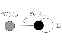
Figure 1: The moose diagram representing the low-energy EFT description of the model in Eq. (2.1.2), along the lines of HLS Bando:1984ej ; Casalbuoni:1985kq ; Bando:1987br ; Casalbuoni:1988xm ; Harada:2003jx (see also Georgi:1989xy ; Appelquist:1999dq ; Piai:2004yb ; Franzosi:2016aoo ). The two sites represent the $SU(4)_{A}\times SU(4)_{B}$ global symmetry. The scalar $S$ transforms on the bifundamental representation, while $\Sigma$ is antisymmetric. The $SU(4)_{A}$ group is gauged with coupling $g_{\rho}$, while the $SU(2)_{L}\times U(1)_{Y}$ SM subgroup of $SU(4)_{B}$ can be weakly gauged, with couplings $g$ and $g^{\prime}$. In most of this paper we set $g=0=g^{\prime}$, and hence ignore the interactions of the strongly coupled dynamics with the standard-model fields.

The full set of $\rho$ and $a_{1}$ mesons spans the adjoint representation of the global $SU(4)$ symmetry. An EFT description of their long-distance dynamics can be built starting from the diagram in Fig. 1. The $15$ spin-1 fields are introduced as gauge fields of $SU(4)_{A}$. Two scalars, the antisymmetric $\Sigma$ of $SU(4)_{A}$, and the bi-fundamental $S$, transform as

$$\Sigma\,\rightarrow\,U_{A}\Sigma U_{A}^{T}\,,~{}~{}~{}~{}~{}S \rightarrow U_{B}\,S\,U_{A}^{\dagger}\,,$$ (16)

under the action of $U_{A}\in SU(4)_{A}$ and $U_{B}\in SU(4)_{B}$. The VEV of $S$ breaks the enlarged symmetry and provides mass for all the vectors. $S$ is subject to the constraints $S^{\dagger}S=\mathbb{I}_{4}$, that are solved by parametrising $S=e^{\frac{2i\sigma}{F}}$, with $\sigma=\sigma^{A}T^{A}$ and $F$ the decay constant. At the same time, we parametrise $\Sigma=e^{\frac{2i\pi}{f}}\Omega$, in such a way that the two scalars together implement the breaking $SU(4)_{A}\times SU(4)_{B}\rightarrow Sp(4)$, and describe the $15$ exact Goldstone bosons that are higgsed away into the longitudinal components of the massive spin-1 states, as well as the remaining $5$ (massive) PNGB, denoted as $\bar{\pi}^{A}$ in the following.

In composite Higgs models, the SM gauge group $SU(2)_{L}\times U(1)_{Y}$ is a subgroup of $SU(4)_{B}$, and it is chosen to be a subgroup of the unbroken global $Sp(4)$. The covariant derivative of $S$ is given by

$$D_{\mu}S = \partial_{\mu}S+i\left(gW_{\mu}+g^{\prime}B_{\mu}\right)S-iSg_{\rho}A_{\mu}\,,$$ (17)

with $A_{\mu}=A_{\mu}^{A}T^{A}$ and $T^{A}$ the generators of $SU(4)_{A}$, while $W_{\mu}=W_{\mu}^{i}t_{L}^{i}$ and $B_{\mu}$ are the gauge bosons of $SU(2)_{L}\times U(1)_{Y}$. The covariant derivative of $\Sigma$ is

$$D_{\mu}\Sigma = \partial_{\mu}\Sigma+i\left[\frac{}{}(g_{\rho}A_{\mu})\Sigma\,+\,\Sigma(g_{\rho}A_{\mu})^{T}\right]\,$$ (18)

$$= \left\{\partial_{\mu}e^{\frac{2i\pi}{f}}+i\left[\frac{}{}(g_{\rho}A_{\mu})e^{\frac{2i\pi}{f}}\,-\,e^{\frac{2i\pi}{f}}\Omega(g_{\rho}A_{\mu})^{T}\Omega\right]\right\}\Omega\,,$$ (19)

where we have made use of the fact that $\Omega^{2}=-\mathbb{I}_{4}$. From this point onwards, we set $g=0=g^{\prime}$, and focus on the dynamics of the strongly-coupled new sector in isolation from the SM fields.

We write the Lagrangian density describing the $15$ gauge bosons $A_{\mu}^{A}$, as well as the $20$ pseudo-scalar fields $\pi^{A}$ and $\sigma^{A}$, as

$${\cal L} = -\frac{1}{2}{\rm Tr\,}\left.A_{\mu\nu}A^{\mu\nu}-\frac{\kappa}{2}{\rm Tr\,}\left\{A_{\mu\nu}\Sigma(A^{\mu\nu})^{T}\Sigma^{\ast}\right\}\right.$$

$$+\frac{f^{2}}{4}{\rm Tr\,}\left\{\frac{}{}D_{\mu}\Sigma\,(D^{\mu}\Sigma)^{\dagger}\right\}\,+\,\frac{F^{2}}{4}{\rm Tr\,}\left\{\frac{}{}D_{\mu}S\,(D^{\mu}S)^{\dagger}\right\}$$

$$+b\frac{f^{2}}{4}{\rm Tr\,}\left\{D_{\mu}(S\Sigma)\left(D^{\mu}(S\Sigma)\right)^{\dagger}\right\}\,+\,c\frac{f^{2}}{4}{\rm Tr\,}\left\{D_{\mu}(S\Sigma S^{T})\left(D^{\mu}(S\Sigma S^{T})\right)^{\dagger}\right\}\,$$

$$-\frac{v^{3}}{8}{\rm Tr\,}\left\{\frac{}{}M\,S\,\Sigma\,S^{T}\right\}\,+\,{\rm h.c.}$$

$$-\frac{v_{1}}{4}{\rm Tr\,}\left\{\frac{}{}M\,(D_{\mu}S)\,\Sigma\,(D^{\mu}S)^{T}\right\}\,-\frac{v_{2}}{4}{\rm Tr\,}\left\{\frac{}{}M\,S\,(D_{\mu}\Sigma)\,(D^{\mu}S)^{T}\right\}\,+\,{\rm h.c.}\,$$

$$-\frac{y_{3}}{8}{\rm Tr\,}\left\{A_{\mu\nu}\Sigma\left[(A^{\mu\nu})^{T}S^{T}MS-S^{T}MSA^{\mu\nu}\right]\right\}\,+\,{\rm h.c.}$$

$$-\frac{y_{4}}{8}{\rm Tr\,}\left\{A_{\mu\nu}\Sigma\left[(A^{\mu\nu})^{T}S^{T}MS+S^{T}MSA^{\mu\nu}\right]\right\}\,+\,{\rm h.c.}\,$$

$$-\frac{v_{5}^{2}}{128}\left({\rm Tr\,}MS\Sigma S^{T}\,+\,{\rm h.c.}\frac{}{}\right)^{2}\,.$$

The first line of Eq. (2.1.2) depends on the field-strength tensor $A_{\mu\nu}$ of the gauge group, and includes the symmetry-breaking term controlled by $\kappa$, that would be omitted from the linear-sigma model version of the same EFT. The covariant derivatives of combinations of $S$ and $\Sigma$ are defined in the obvious way, generalising the covariant derivatives of $S$ and $\Sigma$. The mass deformations are introduced via a new spurion $M$ and via combination of fields such as $S\Sigma S^{T}$, that transforms as $S\Sigma S^{T}\rightarrow U_{B}S\Sigma S^{T}U_{B}^{T}$. The spurion differs from the one in the chiral Lagrangian as it formally transforms as $M\rightarrow U_{B}^{\ast}MU_{B}^{\dagger}$. In this way the whole Lagrangian is manifestly $SU(4)_{A}$ gauge invariant.

In the expansion, we include two sets of operators. We call leading order (LO) the ones appearing in the first four lines, controlled by the parameters $F$, $f$, $b$, $c$, $\kappa$, $g_{\rho}$ and $v$. This is an exhaustive set of operators, at this order. We call next-to-leading order (NLO) those in the last four lines, controlled by the parameters $v_{1}$, $v_{2}$, $y_{3}$, $y_{4}$ and $v_{5}$. As we will discuss shortly, the list of NLO operators is incomplete. In total there are $12$ parameters. This Lagrangian has to be used with caution. The appearance of $\rho$ and $a_{1}$ fields in the EFT is fully justified only if the coupling $g_{\rho}$ is small, which must be discussed a posteriori, yet is expected to hold in the large-$N$ limit, and as long as $m$ is small.

The last four lines of Eq. (2.1.2) contain terms that are sub-leading in the power-counting. Because we are going to perform lattice simulations at finite mass $m$, a priori we do not know how important such terms are, and hence we include them. While non-vanishing values of $m$ are allowed within the composite-Higgs framework, the EFT is useful only when $m$ is small enough that truncating at this order is justified.

We do not include the full set of sub-leading four-derivative terms, because they are not important for our current purposes. These terms would become important when a complete analysis of 3-point and 4-point functions is performed, for example. We also omit topological terms. Furthermore, we do not include in $\cal L$ terms with the structure of Eq. (14), such as

$${\rm Tr\,}\left\{\frac{}{}M\,S\,\Sigma\,S^{T}\right\}{\rm Tr\,}\left\{D_{\mu}(S\Sigma S^{T})\left(D^{\mu}(S\Sigma S^{T})\right)^{\dagger}\right\}\,.$$ (21)

We will comment later in the paper on the implications of all these omissions.

We conclude this subsection with a technical comment. Some of the terms in the Lagrangian density in Eq. (2.1.2) involve only nearest-neighbour interactions, in the sense of the diagram in Figure 1, while other couplings introduce non-nearest-neighbour interactions. Such additional interactions might for example emerge from the process of integrating out heavier degrees of freedom. One of the big limitations of the HLS language is that the number of independent, admissible such non-nearest-neighbour interactions grows rapidly with the number of fields in the theory, and hence by introducing more resonances the EFT Lagrangian density loses predictive power because of the proliferation of new free parameters. In the special Lagrangian we wrote, such interactions are controlled by the parameters $\kappa$, $b$, $c$, as well as $v$, $v_{1}$, $v_{2}$, $y_{3}$, $y_{4}$ and $v_{5}$. If only nearest-neighbour couplings were to be allowed, the set of parameters would be restricted to just $f$, $F$ and $g_{\rho}$, at this order in the expansion.

2.1.3 2-point functions

To compute masses and decay constants of the mesons, we use the language of the $SU(2)^{t}_{L}\times SU(2)^{t}_{R}$ symmetry that would be of direct relevance if we were to treat this as a Technicolor model. In particular, this symmetry is not a subgroup of the unbroken $Sp(4)$ global symmetry, and the condensate breaks it. We treat this as a technical tool, that is convenient in order to extract physical quantities from the correlation functions. Yet our results hold also for finite $m$, and apply as well to the composite-Higgs scenario, as we never include in the calculations the effects of the couplings to the external (weakly-coupled) SM fields. The Left-Left current-current correlator is (see Appendix B)

$$\Sigma(q^{2}) = f_{0}^{2}+\frac{M_{\rho}^{2}f_{\rho}^{2}}{q^{2}-M_{\rho}^{2}}+\frac{M_{a_{1}}^{2}f_{a_{1}}^{2}}{q^{2}-M_{a_{1}}^{2}}\,,$$ (22)

from which one can read that the masses and decay constants are given by

$$M_{\rho}^{2} = \frac{1}{4(1+\kappa+m\,y_{3})}{g_{\rho}}^{2}\left(bf^{2}+F^{2}+2mv_{1}\right)\,,$$ (23)

$$M_{a_{1}}^{2} = \frac{1}{4(1-\kappa-m\,y_{4})}{g_{\rho}}^{2}\left(bf^{2}+F^{2}+2mv_{1}\right)+$$

$$+\frac{g_{\rho}^{2}}{1-\kappa-m\,y_{4}}\left(f^{2}+m(v_{2}-v_{1})\right)\,,$$

$$f_{\rho}^{2} = \frac{1}{2}\left(bf^{2}+F^{2}+2mv_{1}\right)\,,$$ (25)

$$f_{a_{1}}^{2} = \frac{\left(bf^{2}-F^{2}+2m(v_{1}-v_{2})\right)^{2}}{2\left((b+4)f^{2}+F^{2}-2mv_{1}+4mv_{2}\right)}\,,$$ (26)

$$f_{0}^{2} = \frac{}{}F^{2}+(b+2c)f^{2}\,.$$ (27)

and that the pion decay constant is

$$f_{\pi}^{2}(0) = \lim_{q^{2}\rightarrow 0}\Sigma(q^{2})\,=\,f_{0}^{2}-f_{\rho}^{2}-f_{a_{1}}^{2}\,.$$ (28)

As anticipated, the notation explicitly specifies that $f_{\pi}^{2}(0)$ is extracted from 2-point functions evaluated at $q^{2}=0$. The fact that $f_{0}^{2}=f_{\pi}^{2}(0)+f_{\rho}^{2}+f_{a_{1}}^{2}$ is independent of $m$ is the accidental consequence of the truncation we made, in particular of the omission of the operator in (21). Whether or not this is justified, depends on the range of $m$ considered and on the size of the EFT coefficients, as emerging from lattice data.

One can compute the right-hand-side of the first and second Weinberg sum rules, within the EFT, to obtain

$$f_{a_{1}}^{2}-f_{\rho}^{2}+f_{\pi}^{2}(0) = 2(cf^{2}-mv_{1})\,,$$ (29)

$$f_{\rho}^{2}M_{\rho}^{2}-f_{a_{1}}^{2}M_{a_{1}}^{2} = \frac{g_{\rho}^{2}}{8}\left(\frac{(-b{f^{2}}+{F^{2}}+2{m}({v_{2}}-{v_{1}}))^{2}}{\kappa+{m}{y_{4}}-1}+\frac{(b{f^{2}}+{F^{2}}+2{m}{v_{1}})^{2}}{\kappa+{m}{y_{3}}+1}\right),$$ (30)

hence showing explicitly that the non-nearest-neighbour couplings $b$, $c$, $\kappa$, $y_{4}$, $y_{3}$, $v_{1}$ and $v_{2}$ yield to direct violations of the Weinberg sum rules, within the EFT. As anticipated, this is not surprising: non-nearest-neighbour interactions are expected to emerge from integrating out heavy degrees of freedom, and result in the violation of the Weinberg sum rules because their rigorous derivation involves summing over all possible resonances. The additional couplings, in effect, parameterise the contribution to the sum rules of heavier resonances that have been omitted.

2.1.4 Pion mass and $g_{\rho\pi\pi}$ coupling

To compute the physical mass and couplings of the pions, it is convenient to fix the unitary gauge, by setting $\sigma^{A}=0$ along the unbroken $A=6\,,\,\cdots\,,\,15$ generators, and

$$\sigma^{A} = S\bar{\pi}^{A}\,=\,\ \frac{((2+b)f+mv_{2}/f)F}{\cal N}\bar{\pi}^{A}\,,$$ (31)

$$\pi^{A} = C\bar{\pi}^{A}\,=\,\frac{F^{2}-bf^{2}-2m(v_{1}-v_{2})}{\cal N}\bar{\pi}^{A}\,,$$ (32)

for $A=1\,,\,\cdots\,,\,5$ along the broken generators, with the normalisation factor ${\cal N}$ chosen so that the physical $\bar{\pi}^{A}$ are canonically normalised:

$${\cal N}^{2} = \frac{\left((b+4)f^{2}+F^{2}-2m{v_{1}}+4m{v_{2}}\right)}{f^{2}}\left\{2f^{2}m{v_{2}}(b+2c)-m^{2}{v_{2}}^{2}+\frac{}{}\right.$$

$$\left.\frac{}{}+f^{2}\left(bcf^{2}-2m{v_{1}}(b+c+1)+bf^{2}+bF^{2}+4cf^{2}+cF^{2}+F^{2}\right)\right\}\,.$$

The $5$ degenerate pions have mass

$$m^{2}_{\pi} = \left(\frac{}{}mv^{3}+m^{2}v_{5}^{2}\right)\frac{((4+b)f^{2}+F^{2}-2mv_{1}+4mv_{2})^{2}}{2f^{2}{\cal N}^{2}}\,,$$ (34)

which modifies the GMOR relation to read

$$m_{\pi}^{2}f_{\pi}^{2}=m(v^{3}+mv_{5}^{2})\,.$$ (35)

The $g_{\rho\pi\pi}$ coupling is conventionally defined by the Lagrangian density

$${\cal L}_{\rho\pi\pi} = -2ig_{\rho\pi\pi}{\rm Tr\,}\left(\frac{}{}\rho^{\mu}[\partial_{\mu}\bar{\pi}\,,\,\bar{\pi}]\right)\,,$$ (36)

so that the width (at tree level) is $\Gamma_{\rho}=\frac{g^{2}_{\rho\pi\pi}}{48\pi}M_{\rho}\,\left(1-4\frac{m_{\pi}^{2}}{M_{\rho}^{2}}\right)^{3/2}$. We find that

$$g_{\rho\pi\pi} = \frac{{g_{\rho}}}{2f^{2}{\cal N}^{2}\sqrt{1+\kappa+m\,y_{3}}}\left\{\frac{}{}m^{2}v_{2}^{2}\left((5b-8)f^{2}-3F^{2}+10mv_{1}\right)\right.$$ (37)

$$\left.+(b+2)f^{2}\left(\left(2f^{2}+F^{2}\right)\left(bf^{2}+F^{2}\right)\right.\right.$$

$$\left.\left.-2mv_{1}\left(2(b+1)f^{2}+F^{2}\right)\right)+2mv_{2}\left(2b(b+3)f^{4}+mv_{1}\left(F^{2}-3bf^{2}\right)\right.\right.$$

$$\left.\left.+2(b+1)f^{2}F^{2}-2m^{2}v_{1}^{2}\right)-8m^{3}v_{2}^{3}\frac{}{}\right\}\,.$$

We conclude with a comment about unitarity. While the calculations performed here make use of the unitary gauge, we must check that the kinetic terms of all the Goldstone bosons be positive before setting to zero the linear combinations providing the longitudinal components of the vectors. We call the relevant normalisations $k_{10}$, $k_{5}$ and $k_{5}^{\prime}$, coming from the kinetic term of $\sigma^{A}$ with $A>5$, as well as the trace and the determinant of the kinetic matrix mixing $\sigma^{A}$ and $\pi^{A}$ with $A<6$. Such combinations are explicitly given by:

$$k_{10} = \frac{bf^{2}+F^{2}+2m{v_{1}}}{F^{2}}\,,$$

$$k_{5} = 2+b+c+(b+4c)\frac{f^{2}}{F^{2}}-2mv_{1}\,,$$ (38)

$$k_{5}^{\prime}F^{2} = b\left((c+1)f^{2}+F^{2}-2mv_{1}+2mv_{2}\right)+$$

$$+c\left(4f^{2}+F^{2}-2mv_{1}+4mv_{2}\right)-\frac{m^{2}v_{2}^{2}}{f^{2}}+F^{2}-2mv_{1}\,.$$

We require that $k_{10},k_{5},k_{5}^{\prime}>0$. Furthermore, for the kinetic terms of the vectors to be positive definite one must impose $\kappa+m\,y_{4}<1$ and $\kappa+m\,y_{3}>-1$.

2.1.5 On the regime of validity of the EFT

In the EFT we wrote to include the $\rho$ and $a_{1}$ particles, we are making use of several expansions. Besides the derivative expansion and the expansion in the mass of the fermions $m$, appearing also in the chiral Lagrangian, there is a third expansion, that involves the coupling $g_{\rho}$ and deserves discussing in some detail.

From lattice calculations of 2-point functions, one extracts the decay constants of $\pi$, $\rho$ and $a_{1}$, in addition to the masses. In the $m=0$ limit, the expressions for the five quantities $M_{\rho}$, $M_{a_{1}}$, $f_{\rho}$, $f_{a_{1}}$ and $f_{\pi}$ depend on the six free parameters $f$, $F$, $b$, $c$, $\kappa$ and $g_{\rho}$, that hence cannot all be determined. Let us choose to leave $\kappa$ undetermined, for example, and solve the algebraic relations for the other five parameters in terms of the physical quantities. The $g_{\rho\pi\pi}$ coupling can then be written as

$$\lim_{m\rightarrow 0}g_{\rho\pi\pi}^{2} = \lim_{m\rightarrow 0}\frac{M_{\rho}^{2}(f_{\rho}^{2}M_{a_{1}}^{2}(-1+\kappa)+f_{a_{1}}^{2}M_{\rho}^{2}(1+\kappa))^{2}}{2f_{\pi}^{4}f_{\rho}^{2}M_{a_{1}}^{4}(1-\kappa)^{2}}\,.$$ (39)

If one were restricted to the massless theory, only by gaining access to 3-point functions could one measure $\kappa$. Yet, detailed information about the $m$-dependence of 2-point functions can be used to predict $g_{\rho\pi\pi}$, and the width of the $\rho$ meson. In principle, the width of the $\rho$ meson $\Gamma_{\rho}$ could be compared with the physical width extracted from lattice calculations Luscher:1991cf ; Feng:2010es . In this way we would be able to adjudicate explicitly whether the weak-coupling assumption that underpins this EFT treatment is justified. However, the direct extraction of $\Gamma_{\rho}$ from lattice data is highly non-trivial, and will require a future dedicated study.

There is no reason a priori to expect that $g_{\rho}$, or $g_{\rho\pi\pi}$, be small, except in the large-$N$ limit. The fact that from 2-point functions we can infer some of the properties of the EFT that enter the 3-point functions holds only provided the coupling is small, with $g_{\rho\pi\pi}^{2}/(48\pi)\ll 1$. Furthermore, if $M_{\rho}$ and $M_{a_{1}}$ happen to be large in respect to $f_{\pi}$, bringing them close to the natural cut-off set by the derivative expansion, it would again signal a break-down of the perturbative expansion within the EFT.

Nevertheless, even in the regime of large $g_{\rho}$, we can still learn something from the expansion in small mass $m$. In particular, we should be able to use the EFT to reproduce the $m$-dependence of masses and decay constants, at least in the small-$m$ regime. In the future, we envision repeating the study performed in the following sections for $Sp(2N)$ theory with dynamical fermionic matter, and with larger values of $N$, and hence track the $N$-dependence of the individual coefficients.

2.2 Spin${-}1/2$ composite fermions and the top partner

In composite-Higgs models, the generation of the SM fermion masses is often supplemented by the mechanism of partial compositeness (PC). The SM fermions, in particular the top quark, mix with spin-$1/2$ bound states emerging from the novel strong-interaction sector (the composite sector), and phenomenologically this allows both to enhance the fermion mass (as in precursor top-color models) and to trigger electroweak symmetry breaking via vacuum (mis)alignement. As an example, we borrow some of the construction in Katz:2005au and Barnard:2013zea . So many other, equally compelling, examples exist in the literature, that we refer the reader to the review Panico:2015jxa and to the references therein.

Let us assume that the microscopic theory admits the existence of $Sp(4)$-colour singlet operators $\hat{\Psi}_{i}$ and $\hat{\Psi}^{c}_{i}$, that have spin-$1/2$, carry $SU(3)_{c}$ colour and, combined, span vectorial representations of the SM gauge group. The index $i=1,2$ refers to the $SU(2)_{L}$ singlets and doublets, respectively, and the notation refers to the fact that we write the operators as 2-component fermions. Let us now consider the low-energy description of the lightest particles excited from the vacuum by such operators, and write it in terms of new 2-component spinorial fields $\Psi_{i}$ and $\Psi^{c}_{i}$ with the same quantum numbers as $\hat{\Psi}_{i}$ and $\hat{\Psi}^{c}_{i}$. Coarse-graining over model-dependent details, $\Psi_{i}$ and $\Psi^{c}_{i}$ have the correct quantum numbers to couple to the SM quarks, in particular to the SM top quark, represented by the 2-component Weyl fermions $t$ and $t^{c}$, provided $\Psi_{i}$ transforms on the fundamental of $SU(3)_{c}$ and $\Psi^{c}_{i}$ on its conjugate.

Below the electroweak symmetry-breaking scale $v_{W}$, the mass terms take the form

$${\mathcal{L}}^{{\mathrm{mix}}} = -\frac{1}{2}\left\{\lambda_{1}M_{\ast}\left(\frac{M_{\ast}}{\Lambda}\right)^{d_{\Psi}-5/2}\Psi_{1}^{T}\tilde{C}t^{c}+\lambda_{2}M_{\ast}\left(\frac{M_{\ast}}{\Lambda}\right)^{d_{\Psi^{c}}-5/2}t^{T}\tilde{C}\Psi_{2}^{c}+\right.$$ (40)

$$\left.+\lambda M_{\ast}\left[\Psi_{1}^{T}\tilde{C}\Psi_{1}^{c}\frac{}{}+\,\Psi_{2}^{T}\tilde{C}\Psi_{2}^{c}\right]+yv_{W}\left[\Psi_{1}^{T}\tilde{C}\Psi_{2}^{c}\frac{}{}+\,\Psi_{2}^{T}\tilde{C}\Psi_{1}^{c}\right]^{\frac{}{}}\right\}\,+\,{\mathrm{h.c.}}\,,$$

where $\lambda_{1}$, $\lambda_{2}$, $\lambda$ and $y$ are dimensionless couplings, $M_{\ast}$ represents the typical scale of the masses of composite fermions in the $Sp(4)$ gauge theory and $\Lambda$ represents the underlying scale at which (third-generation) flavour physics arises (see also Katz:2005au ). $d_{\Psi}=d_{\Psi^{c}}$ is the dimension of the operators $\hat{\Psi}$ and $\hat{\Psi}^{c}$ in the underlying theory.

Diagonalisation of the resulting mass matrix, under the assumption that $yv_{W}$ be small in respect to the other scales, yields two heavy Dirac masses approximately given by

$$m^{2}_{1} \simeq \left(\lambda^{2}\,+\,\lambda_{1}^{2}\left(\frac{M_{\ast}}{\Lambda}\right)^{2d_{\Psi}-5}\right)M_{\ast}^{2}\,,$$ (41)

$$m^{2}_{2} \simeq \left(\lambda^{2}\,+\,\lambda_{2}^{2}\left(\frac{M_{\ast}}{\Lambda}\right)^{2d_{\Psi^{c}}-5}\right)M_{\ast}^{2}\,,$$ (42)

and finally the mass (squared) of the top is given approximately by

$$m_{t}^{2} \simeq \frac{\lambda_{1}^{2}\lambda_{2}^{2}y^{2}\left(\frac{M_{\ast}}{\Lambda}\right)^{2d_{\Psi}+2d_{\Psi^{c}}-10}v_{W}^{2}M_{\ast}^{4}}{m_{1}^{2}m_{2}^{2}}\,.$$ (43)

In order to assess the viability of these models, one needs to provide a microscopic origin for all of the parameters appearing in Eq. (40). To do so, one must specify the (model-dependent) microscopic details controlling the nature of the composite fermions. Spin-$1/2$ composite $Sp(4)$-neutral particles arise in the presence of fermions in higher-dimensional irreducible representations. As an example, ref. Barnard:2013zea proposes to extend the field content of the microscopic theory in Table 1 to include 2-component elementary fermions $\chi$ (and $\chi^{c}$) in the antisymmetric representation of the gauge $Sp(4)$, transforming as singlets of the global $SU(4)$, and on the fundamental (and anti-fundamental) representation of the $SU(3)_{c}$ gauge symmetry of QCD.

The $\chi$ and $\chi^{c}$ fermions carry QCD colour charge, which allows to construct coloured composite states in the antisymmetric, six-dimensional representation of the global $SU(4)$ group, by coupling them to a pair of fundamental fermions $q$. For example, the operators $\hat{\Psi}$ and $\hat{\Psi}^{c}$ aforementioned can be obtained as

$$\hat{\Psi}^{ab\alpha}\equiv\left(q^{a}\chi^{\alpha}q^{b}\right)\,,\\ \hat{\Psi}^{c\,ab}_{\alpha}=\left(q^{a}{\chi}^{c}_{\alpha}q^{b}\right)\,,$$ (44)

where summations over $Sp(4)$ gauge indices are understood, while we show explicitly the (antisymmetrised) global $SU(4)$ indices $a$ and $b$, and the $SU(3)_{c}$ colour index $\alpha$.

One of our long-term goals is to study the PC mechanism with lattice simulations, which requires generalising the lattice study we will report upon in the following sections to the case in which the field content contains at least two species of fermions transforming in different representations of the fundamental gauge group. The example we outlined here, though incomplete, immediately highlights how, from the phenomenological perspective, the determination of the masses of the top partners (the scale $M_{\ast}$ and couplings such as $\lambda$, as a function of the elementary-fermion mass $m$) in the PC mechanism are of direct interest, as they represent a way to test the theory. At the same time, they are accessible on the lattice, even without introducing (model-dependent) couplings to the SM fields.

The other additional, essential, input from non-perturbative dynamics of the microscopic theory is the anomalous dimension of the top-partner operators, such as $\hat{\Psi}$ and $\hat{\Psi}^{c}$ in the example. For the PC mechanism to be valid, in principle one needs the operator dimensions to be small, for example $d_{\Psi}\leq 5/2$, which implies that the operator $\hat{\Psi}_{1}^{T}\tilde{C}t^{c}$ is relevant in the IR, and that the anomalous dimensions of the candidate operators have to be non-perturbatively large. In practice, since $\Lambda/M_{\ast}$ is not infinity, this requirement may be relaxed, at the price of admitting some degree of fine-tuning.

Finally, the (model-dependent) extension of the field content, required by the PC mechanism, also implies the enlargement of the global symmetry, and additional light PNGB’s, some of which are neutral, some of which carry $SU(3)_{c}$ colour, and many of which may be lighter than the typical scale of the other composite particles. Lattice calculations of the masses of such particles would offer the opportunity to connect with the phenomenology derived from direct particle searches at the LHC.

3 Numerical lattice treatment

In this Section, we present the discretised Euclidean action and Monte Carlo techniques used in the numerical studies. We adapt the state-of-the-art lattice techniques established for QCD to the two-flavour $Sp(4)$ theory. Pioneering lattice studies of $Sp(4)$ gauge theory without matter can be found in Holland:2003kg . Numerical calculations are carried out by modifying the HiRep code DelDebbio:2008zf .

3.1 Lattice action

For the numerical study of $Sp(2N)$ gauge theory on the lattice, we consider the standard plaquette action

$$S_{g}[U]=\beta\sum_{x}\sum_{\mu<\nu}\left(1-\frac{1}{2N}\textrm{Re}~{}\textrm{Tr}\ \mathcal{P}_{\mu\nu}(x)\right),$$ (45)

where $\beta=4N/g^{2}$ is the lattice bare gauge coupling, and $N=2$ in the $Sp(4)$ case of this paper. The plaquette $\mathcal{P}_{\mu\nu}$ is given by

$$\mathcal{P}_{\mu\nu}(x)=U_{\mu}(x)U_{\nu}(x+\hat{\mu})U_{\mu}^{\dagger}(x+\hat{\nu})U_{\nu}^{\dagger}(x)\,,$$ (46)

where the link variables $U_{\mu}(x)$ are $Sp(4)$ group elements in the fundamental representation, while $\hat{\mu}$ and $\hat{\nu}$ are unit vectors along the $\mu$ and $\nu$ directions.

In the dynamical simulations with two Dirac fermions in the fundamental representation, we use the (unimproved) Wilson action

$$S_{f}[U,\bar{\psi},\psi]=a^{4}\sum_{x}\bar{\psi}(x)D_{m}\psi(x)\,,$$ (47)

where the massive Wilson-Dirac operator is given by

$$D_{m}\psi(x) \equiv (D+m_{0})\psi(x)$$

$$= (4/a+m_{0})\psi(x)-\frac{1}{2a}\sum_{\mu}\left\{\frac{}{}(1-\gamma_{\mu})U_{\mu}(x)\psi(x+\hat{\mu})+\right.$$

$$\left.+(1+\gamma_{\mu})U_{\mu}(x-\hat{\mu})\psi(x-\hat{\mu})\frac{}{}\right\},$$

where $a$ is the lattice spacing and $m_{0}$ is the bare fermion mass.

3.2 Heat Bath

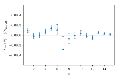
Figure 2: Difference between the averaged plaquette obtained at various values of $\beta$ in this work and in Ref. Holland:2003kg . The symbols $\langle P\rangle$ and $\langle P\rangle_{H.P.W.}$ denote the measurements from this work and those reported in Ref. Holland:2003kg , respectively. Our lattice volume is $V=8^{4}$, and both calculations use the HB algorithm with over-relaxation, as explained in Sec. 3.2. Each point has been obtained from $5000$ measurements, and the errors are corrected for autocorrelations.

As a powerful way to perform calculations in the pure $Sp(4)$ gauge theory, we implemented a heat bath (HB) algorithm with micro-canonical over-relaxation updates, to improve the decorrelation of successive configurations. As in the case of $SU(N)$ Cabibbo:1982zn , the algorithm acts in turn on $SU(2)$ subgroups, the choice of which can be shown to strongly relate to the ergodicity of the update pattern.

A sufficient condition to ensure ergodicity is to update the minimal set of $SU(2)$ subgroups to cover the whole $Sp(2N)$ group. This condition can be suitably translated to the algebra of the group and generalised to any $Sp(2N)$. In the $Sp(4)$ case, of relevance to this paper, we choose to update a redundant set of subgroups, in order to improve the decorrelation of configurations. We provide below a possible partition of the generators used to cover all of the $Sp(4)$ gauge group, written with the notation of Lee:2017uvl .

• $SU(2)_{L}$ subgroup, with generators $T_{L}^{i}$ in Eq. (B.6) of Lee:2017uvl .

• $SU(2)_{R}$ subgroup, with generators $T^{i}_{R}$ in Eq. (B.7) of Lee:2017uvl .

• $SU(2)_{\tau}$ subgroup, with generators expressed in terms of B.4 in Lee:2017uvl :

  $$\tau^{1}=T^{11}\ ;\qquad\tau^{2}=T^{7}\ ;\qquad\tau^{3}=T^{15}\ .$$ (49)

• $SU(2)_{\tilde{\tau}}$ subgroup, with generators expressed in terms of B.4 in Lee:2017uvl :

  $$\tilde{\tau}^{1}=T^{13}\ ;\qquad\tilde{\tau}^{2}=T^{8}\ ;\qquad\tilde{\tau}^{3}=T^{14}\ .$$ (50)

The set of $10$ generators $T^{i}_{L}$, $T^{i}_{R}$, $\tau^{1\,,\,2}$ and $\tilde{\tau}^{1\,,\,2}$ spans the whole $Sp(4)$. The minimal set of $5$ elements that generate the whole group by closure consists for example of any two elements $T^{i}_{L}$, any two elements $T^{j}_{R}$ and one additional element among $\tau^{1\,,\,2}$ and $\tilde{\tau}^{1\,,\,2}$.

As a check of correctness of the algorithm we employed, we compared the average of the elementary plaquette to the results obtained in Holland:2003kg , as shown in Fig. 2, confirming that they are compatible within the statistical errors.

3.3 Hybrid Monte Carlo

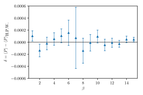
Figure 3: Differences between the average plaquette values $\langle P\rangle$ obtained by using the HMC algorithm described in Sec. 3.3 with heavy quarks ($am_{0}=10.0$) and the HB for pure $Sp(4)$ theories from the literature Holland:2003kg .

In the study of $N_{f}=2$ dynamical Dirac fermions, we make use of the hybrid Monte Carlo (HMC) algorithm. As $Sp(4)$ is a subgroup of $SU(4)$, most of the numerical techniques used for $SU(N)$ with an even number of fermions can straightforwardly be extended to our study. However, there are two distinguishing features.

First of all, in contrast to the HB algorithm, the explicit form of the group generators of ${Sp}(4)$ is necessary for the molecular dynamics (MD) update. For instance, the MD forces for the gauge fields are given by

$$F^{A}_{G}(x,\mu)=-\frac{\beta}{2NT_{F}}{\textrm{Re}}~{}{\textrm{Tr}}[iT^{A}U_{\mu}(x)V^{\dagger}_{\mu}(x)],$$ (51)

where $V_{\mu}(x)$ is the sum of forward and backward staples around the link $U_{\mu}(x)$. The generators $T^{A}$ with $A=6\,,\,\cdots\,,\,15$ are given in Appendix B of Lee:2017uvl . The group invariant $T_{F}$ is defined as ${\rm Tr\,}(T^{A}T^{B})=T_{F}\delta^{AB}$, which in our case yields $T_{F}=1/2$, so that for $Sp(4)$ the normalization is $2NT_{F}=2$.

Secondly, due to machine precision, it is not guaranteed that the link variables stay in the $Sp(4)$ group manifold. In analogy with the re-unitarization process implemented in $SU(N)$ studies, we perform a re-symplectisation at the end of each MD step. We describe in Appendix C the procedure, based on $Sp(4)$ projection that makes use of the quaternion basis.

As a further test of this implementation of the HMC algorithm, we calculated the expectation value of the difference of the auxiliary Hamiltonian at the beginning and the end of a MD trajectory $\langle\Delta H\rangle$ for various values of the integration step size $\epsilon$, in the case with $\beta=6.9$ and $am_{0}=-0.85$ on a $24\times 12^{3}$ lattice. We found that $\langle\Delta H\rangle$ is proportional to $\epsilon^{4}$, as expected for a second order Omelyan integrator Takaishi:1999bi , and Creutz’s equality $\langle\textrm{exp}(-\Delta H)\rangle=1$ Creutz:1988wv is satisfied. We also checked that the average plaquette values are consistent with each other for all values of the step size.

The HiRep code DelDebbio:2008zf is designed to implement $SU(N)$ gauge theories with a generic number of colours and flavours, with fermions in any two-index representation. One of its crucial features is that the gauge group and the representation can be fixed at compile time by using preprocessor macros. This provides us with great flexibility in implementing the aforementioned features of $Sp(4)$.

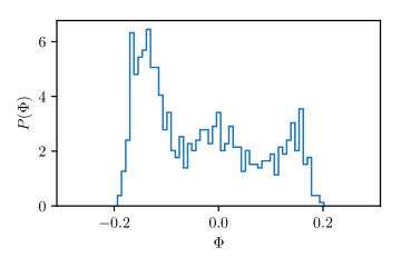
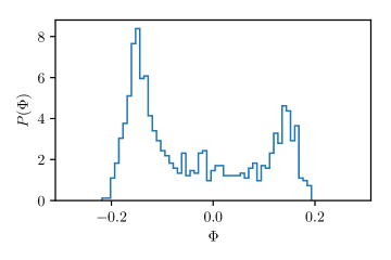
Figure 4: Probability distribution $P(\Phi)$ of the expectation value of the Polyakov loop $\Phi$ averaged over the space-like points, defined in Eq. (52), with the normalisation of $\int d\Phi P(\Phi)=1$, measured on a lattice with size $4\times 12^{3}$, by making use of the HMC algorithm. The lattice couplings are $\beta=7.3$, $7.339$ and $7.345$ (top to bottom panel), roughly corresponding to temperatures $T$ below, at, and above the critical temperature $T_{c}$, respectively.

As a nontrivial test of the HMC code, we first calculate the expectation value of the plaquette of the theory with two degenerate, very heavy fundamental fermions ($a\,m_{0}=10.0$) and compare the results with the pure $Sp(4)$ results from Holland:2003kg . In Fig. 3, we plot the differences of the average plaquette values between the two calculations for various values of $\beta$. The two series are compatible with each other, within the statistical errors.

It is known that the pure $Sp(4)$ theory in $3+1$ dimensions exhibits a first-order deconfinement phase transition Holland:2003kg . Although a finite-size scaling analysis is needed to confirm the existence of the first-order phase transition, for the purpose of a consistency check of the code it is worth showing numerical evidence of the coexistence of the confined and deconfined phases. To this end, we calculate the expectation value of the Polyakov loop averaged over the space-like points, defined by

$$\Phi \equiv \frac{1}{N_{s}^{3}}\sum_{\vec{x}}{\textrm{Tr}}\left(\prod_{t=0}^{N_{t}-1}U_{0}(t,\vec{x})\right).$$ (52)

The temperature $T$ in lattice units is identified with the inverse of the extent of the temporal lattice, $1/N_{t}$. Near the critical temperature $T_{c}$, the probability distribution of $\Phi$ indeed shows the coexistence of two phases, as in the second panel of Fig. 4. In agreement with expectations, the numerical results also show that the expectation value of the Polyakov loop averaged over space is dominated by configurations at $\Phi=0$ in the confining phase (first panel of Fig. 4), while it is dominated by two non-zero values of $\Phi$ in the deconfinement phase (third panel of Fig. 4).

4 Lattice calibration

This Section is devoted to discuss two lattice technicalities that are important in order to extract the correct continuum physics: we address the problem of setting the scale, using the gradient flow, and study the topology of the ensembles generated by our numerical process, to verify that there is no evidence of major problems in the lattice calculations.

4.1 Scale setting and gradient flow

Lattice computations are performed by specifying dimensionless bare parameters in the simulation, and all dimensionful results are extracted in units of the lattice spacing. These results have to be extrapolated to the continuum limit to make impact on phenomenology. It is also desirable to express them in natural units. Such demands make the scale setting an important task in lattice calculations. To carry out this task, the most straightforward approach is to compute a physical quantity on the lattice, and then compare with its experimental measurement. In the absence of experimental results for the $Sp(4)$ gauge theory, one can still accomplish reliable continuum extrapolations by employing a scale defined on theoretical grounds, such that one can determine the ratio $a_{1}/a_{2}$ of the lattice spacings in two simulations performed at different choices of the bare parameters.

The gradient flow in quantum field theories, as revived in recent years by Martin Lüscher in the context of the trivialising map Luscher:2009eq , is a popular method for scale setting Luscher:2010iy ; Luscher:2011bx . To study the gradient flow in a field theory, one first adds an extra dimension, called flow time and denoted by $t$. An important point articulated by Lüscher is that a field theory defined initially with a cut-off can be renormalised at non-vanishing flow time. In addition, choosing carefully the bulk equation governing the gradient flow, the theory does not generate new operators along the flow time (counter-terms), keeping the renormalisation of the five-dimensional theory simple.

The Yang-Mills gradient flow of the gauge field $B_{\mu}(t,x)$ is implemented via the equation

$$\frac{\mathrm{d}B_{\mu}(t,x)}{\mathrm{d}t}=D_{\nu}G_{\nu\mu}(t,x)\,,{\mathrm{with}}\mbox{ }B_{\mu}(t,x)|_{t=0}=A_{\mu}(x),$$ (53)

where $G_{\mu\nu}$ is the field strength tensor associated with $B_{\mu}(t,x)$, $D_{\mu}=\partial_{\mu}+[B_{\mu},\cdot]$ the corresponding covariant derivative, and $A_{\mu}(x)$ the initial gauge field in the four-dimensional theory. Noticing that Eq. (53) describes a diffusion process, the flow time $t$ therefore has length-dimension two. It has been shown that, to all orders in perturbation theory, any gauge invariant composite observable constructed from $B_{\mu}(t,x)$ is renormalised at $t>0$ Luscher:2011bx . In particular, Lüscher demonstrated that the action density can be related to the renormalised coupling, $\alpha(\mu)$, at the leading order in perturbation theory through

$$\alpha(\mu)=k_{\alpha}t^{2}\langle E(t)\rangle\equiv k_{\alpha}{{\mathcal{E}}}(t)\,,$$ (54)

with $\mu=\frac{1}{\sqrt{8t}}$, and

$$E(t)=-\frac{1}{2}{\rm Tr}(G_{\mu\nu}G_{\mu\nu})\,.$$ (55)

The dimensionless constant $k_{\alpha}$ is analytically computable Luscher:2010iy . Equation (54) can actually serve as the definition of a renormalisation scheme: the gradient-flow (GF) scheme. Furthermore, since $t^{2}\langle E(t)\rangle\equiv{{\mathcal{E}}}$ is proportional to the GF-scheme coupling, this quantity can be used to set the scale. In other words, if one imposes the condition

$${{\mathcal{E}}}(t)|_{t=t_{0}}={{\mathcal{E}}}_{0}\,,$$ (56)

where ${{\mathcal{E}}}_{0}$ is a constant that one can choose, then $\sqrt{t_{0}}$ should be a common length scale, assuming lattice artefacts are under control. In practice, one measures $\sqrt{t_{0}}$ in lattice units. That is, one computes $\sqrt{t_{0}}/a\equiv\sqrt{\hat{t}_{0}}$. This allows the determination of the ratio of lattice spacings from simulations performed at different values of the bare parameters.

It is worth mentioning that the diffusion radius in Eq. (53) is $\sqrt{8t}$, and it is convenient to define the ratio

$$c_{\tau}=\sqrt{8t}/L\,,$$ (57)

where $L$ is the lattice size.

Given that the right-hand side of Eq. (53) is the gradient of the Yang-Mills action, the most straightforward way to latticise it is

$$\frac{\partial V_{\mu}(t,x)}{\partial t}=-g_{0}^{2}\left\{\partial_{x,\mu}S^{({\mathrm{flow}})}_{{\mathrm{latt}}}\left[V_{\mu}\right]\right\}V_{\mu}(t,x),\mbox{ }\mbox{ }V_{\mu}(0,x)=U_{\mu}(x)\,,$$ (58)

where $V_{\mu}(t,x)$ is the gauge link at flow time $t$, and $S^{({\mathrm{flow}})}_{{\mathrm{latt}}}$ is a lattice gauge action. Notice that $S^{({\mathrm{flow}})}_{{\mathrm{latt}}}$ does not have to be the same as the gauge action used in the Monte Carlo simulations. We employ the Wilson flow where $S^{({\mathrm{flow}})}_{{\mathrm{latt}}}$ is the Wilson plaquette action.

The gradient flow serves as a smearing procedure for the gauge fields. This means the larger the flow time, the smoother the resultant gauge configurations will be. In other words, the larger the flow time is, the smaller the ultraviolet fluctuations of flown observables. On the other hand, it also means the gauge fields become more extended objects as the flow time grows. This results in longer autocorrelation time, and makes the statistics worse. Furthermore, having $c_{\tau}>0.5$ can lead to significant finite-volume effects. These are issues one would have to consider carefully when choosing a value for the constant ${{\mathcal{E}}}_{0}$ in Eq. (56).

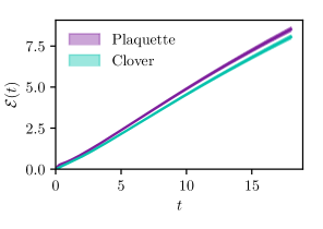
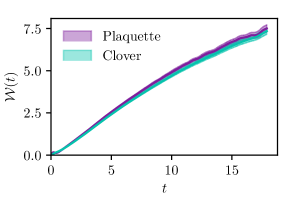
Figure 5: The Wilson flow functions ${{\mathcal{E}}}(t)$ in Eq. (54) (left panel) and ${{\mathcal{W}}}(t)$ in Eq. (59) (right panel) for $N_{\mathrm{f}}=2$, $\beta=6.9$, $am_{0}=-0.90$ and $L=12$, as a function of the flow time $t$, computed by using the methods described in Sec. 4.1.

The action density ${{\mathcal{E}}}(t)$ at non-vanishing flow time is obtained from the diffusion process in Eq. (58), starting from the bare gauge fields. To further reduce the cut-off effects in the scale-setting procedure, an alternative quantity was proposed in Ref. Borsanyi:2012zs . Define

$${{\mathcal{W}}}(t)\equiv t\frac{\mathrm{d}{{\mathcal{E}}}(t)}{\mathrm{d}t}.$$ (59)

Then the scale can be set by

$${{\mathcal{W}}}(t)|_{t=w_{0}^{2}}={{\mathcal{W}}}_{0},$$ (60)

where ${{\mathcal{W}}}_{0}$ is again a dimensionless constant that one can choose.

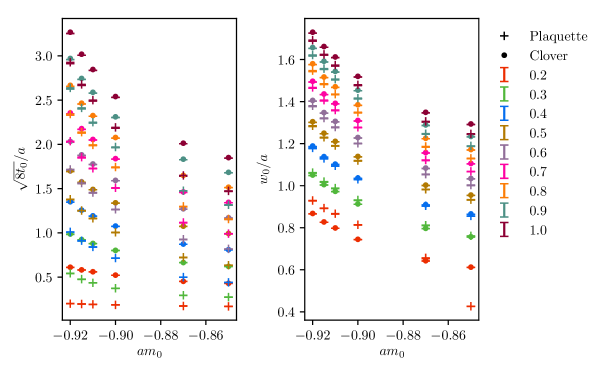
Figure 6: The gradient flow scales $t_{0}$ defined in Eq. (56) (left panel) and $w_{0}$ defined in Eq. (60) (right panel), normalised to the lattice spacing $a$, as a function of the fermion mass $am_{0}$ (on the horizontal axis), for various choices of the scales ${\mathcal{E}}_{0}$ and ${\mathcal{W}}_{0}$, and for the two choices of plaquette or clover (as indicated in the legend). Lattices with size $32\times 16^{3}$ were used for $-0.92\leq am_{0}\leq-0.89$ and $24\times 12^{3}$ for $-0.87\leq am_{0}\leq-0.85$.

On the lattice, the calculation of $E(t)$ depends on a definition of $G_{\mu\nu}$, for which a variety of choices are available. The most obvious is to associate it with the plaquette ${\cal P}_{\mu\nu}$; an alternative is to define a four-plaquette clover, which has a greater degree of symmetry Luscher:2010iy . In the continuum, all definitions should become equivalent, and at finite lattice spacing the relative difference between the two decreases at large $t$. The shape of $E(t)$ at very small $t$ is dominated by ultraviolet effects, and so differs strongly between the two methods; this introduces further constraints into the choice of ${\mathcal{E}}_{0}$. Figure 5 shows ${\mathcal{E}}(t)$ and ${\mathcal{W}}(t)$, calculated both via the plaquette and the clover. As anticipated from Borsanyi:2012zs , the discretisation effects are smaller in ${\mathcal{W}}(t)$ than ${\mathcal{E}}(t)$; this is visible in the splitting between plaquette and clover curves being smaller in the ${\mathcal{W}}(t)$ case.

In the continuum theory, $B_{\mu}(x)$ are elements of the $Sp(4)$ gauge group; however, it is possible that the finite precision of the computer could introduce some numerical artefact that would cause the integrated $B_{\mu}(x)$ to leave the group. Since the integration is an initial value problem, any such artefact introduced would compound throughout the flow, giving potentially significant distortions at large flow time. For this reason we have introduced the re-symplectisation procedure described in Appendix C after each integration step. We find no appreciable difference between the flow with and without re-symplectisation.

We now proceed to set the values of ${\mathcal{E}}_{0}$ and ${\mathcal{W}}_{0}$, such that $t_{0}$ and $w_{0}$ avoid both the regions of finite lattice spacing and finite volume artefacts. In order to obtain a single value for the lattice spacing corresponding to a particular value of $\beta$, and allow comparisons to be drawn with pure gauge theory, we must also be in the vicinity of the chiral limit. Findings in Borsanyi:2012zs indicate that when the fermions are light enough any mass dependence in $w_{0}$ should be small.

Figure 6 shows the fermion-mass dependence in $\sqrt{8t_{0}}$ and $w_{0}$ at $\beta=6.9$, choosing ${\mathcal{E}}_{0}={\mathcal{W}}_{0}\in[0.2,1.0]$. The discretisation effects are significantly smaller in $w_{0}$. We see a relatively strong dependence on the fermion mass in both $t_{0}$ and $w_{0}$; this is contrary to expectations from studies of QCD with light quarks Borsanyi:2012zs . Presently we are studying this fermion-mass dependence. Results of this study will be detailed in future publications. It should be noted that if the behaviour highlighted here persists also in proximity of the chiral limit, extra care will be needed in the process of taking the continuum limit.

4.2 Topological charge history

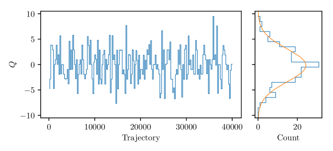
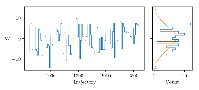
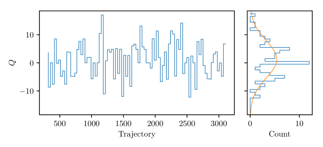
Figure 7: Histories and statistical distributions of the topological charge in Eq. (61) for three selected ensembles. Top to bottom, the figures show the result for the following choices. The pure gauge case, with $\beta=7.62$ and $L=16$ yields the average charge $Q_{0}=-0.17\pm 0.24$ and the standard deviation is $\sigma=3.24\pm 0.24$, with $\chi^{2}/{\rm d.o.f}=0.88$. For $N_{\mathrm{f}}=2$, with $\beta=6.9$, $L=12$ and $am_{0}=-0.85$ we find $Q_{0}=0.23\pm 0.88$ and $\sigma=5.75\pm 0.89$, with $\chi^{2}/{\rm d.o.f}=2.51$. For $N_{\mathrm{f}}=2$ with $\beta=6.9$, $L=16$ and $am_{0}=-0.92$ we obtain $Q_{0}=1.26\pm 0.97$ and $\sigma=6.61\pm 0.98$, with $\chi^{2}/{\rm d.o.f}=1.28$.

As the lattice extent is finite in all directions, a given configuration will fall into one of a number of topological sectors, labelled by an integer (or, at finite $a$, near-integer) topological charge $Q$, which is expected to have a Gaussian distribution about zero. Since it is probabilistically unfavourable to change a discrete global observable using a small local update, $Q$ can show very long autocorrelations; as the continuum limit (i.e. the limit of integer $Q$) is approached, $Q$ can “freeze”, ceasing to change at all.

It is necessary to check that $Q$ is not frozen, and instead moves hergodically, for two reasons. Firstly, the exponential autocorrelation time of the Monte Carlo simulation as a whole scales as one of the longest autocorrelation time in the system (see e.g. Luscher:2011kk ). Secondly, the values of physical observables depend on which topological sector a configuration is in Galletly:2006hq ; sampling a single $Q$ or an unrepresentative distribution of $Q$s will introduce an uncontrolled systematic error. It is therefore necessary to verify that $Q$ not only moves sufficiently rapidly, but also displays the expected Gaussian histogram.

The topological charge $Q$ is computed on the lattice as

$$Q=\sum_{x}q(x)\,,{\rm with}\,\,q(x)=\frac{1}{32\pi^{2}}\epsilon_{\mu\nu\rho\sigma}\operatorname{Tr}\left\{U_{\mu\nu}(x)U_{\rho\sigma}(x)\right\}\,,$$ (61)

and where $x$ runs over all lattice sites. For gauge configurations generated by Monte Carlo studies, this observable is dominated by ultraviolet fluctuations; therefore it is necessary to perform some sort of smoothing to extract the true value. The gradient flow (described in the previous subsection) is used for the purposes of this work.

We have examined the topological charge history for all our existing ensembles, including both pure gauge and those with matter. In most cases, $Q$ is found to move with no noticeable autocorrelation, and shows the expected Gaussian distribution centred on $Q=0$. Samples of these histories are shown in Fig. 7. Some marginal deviation is visible for example in the second of the three series.

5 The spectrum of the Yang-Mills theory

In this Section, we focus our attention on the $Sp(4)$ Yang-Mills theory. We start by reminding the reader about several technical as well as conceptual points related to the physics of glueballs and to the description of confinement in terms of effective string theory. We then summarise the specific methodology we adopt in the process of extracting physical information from the lattice data. We conclude this section by presenting our numerical results on the glueballs, and commenting on their general implications.

5.1 Of glueballs and strings

At zero temperature, $Sp(4)$ Yang-Mills theory is expected to confine. The particle states are colour-singlet gluon bound states, referred to in the literature as glueballs, and labelled by their (integer) spin $J$ and (positive or negative) parity $P$ quantum numbers as $J^{P}$. To distinguish between states with the same $J^{P}$ assignment but different mass, in the superscript of the $n$-th excitation we add $n$ asterisks ($\ast$). For instance, $2^{+\ast\ast}$ denotes the second excitation with $J=2$ and $P=+$, while $2^{+}$ is the ground state in the same channel.

The calculation of the mass spectrum of glueballs requires a fully non-perturbative treatment of the strongly interacting dynamics. We follow the established procedure that extracts glueball masses from the Monte Carlo evaluation of two-point functions of gauge-invariant operators $O(x)$. The operators $O(x)$ transform according to irreducible representations of the rotational group and either commute or anti-commute with the parity operator, hence having well-defined $J^{P}$. Given $O(x)$ defined at any spacetime point $x=(t,\vec{x})$, we separate the space-like and time-like components $\vec{x}$ and $t$, and define the zero-momentum operator $O(t)$ as

$$O(t)=\sum_{\vec{x}}O(t,\vec{x})\ ,$$ (62)

where the sum runs over all spatial points $\vec{x}$ at fixed $t$. The lowest-lying glueball mass in the $J^{P}$ channel is then given by

$$m_{J^{P}}=-\lim_{t\rightarrow\infty}\frac{\log\langle O^{{\dagger}}(0)O(t)\rangle}{t}\,.$$ (63)

Assuming only contributions from poles (an hypothesis that certainly holds at large $N$), we can insert a complete set of single-glueball states $|g_{n}(J,P)\rangle$ carrying the same quantum numbers of $O(t)$ in the correlator $\langle O^{{\dagger}}(0)O(t)\rangle$, and arrive to

$$\langle O^{{\dagger}}(0)O(t)\rangle=\sum_{n}|c_{J^{P},n}|^{2}e^{-m_{J^{P},n}t}\ ,$$ (64)

with $c_{J^{P},n}=\langle g_{n}(J,P)|O(0)|0\rangle$ being the overlap of the state $|g_{n}(J,P)\rangle$ with the state $O(0)|0\rangle$, created by acting with $O(0)$ on the vacuum $|0\rangle$. The correlator $\langle O^{{\dagger}}(0)O(t)\rangle$ contains information not only on the ground state but also on all excitations with non-null overlap with $O(0)|0\rangle$ in the given $J^{P}$ channel.

Glueballs are not the only interesting observables in Yang-Mills theory. In the presence of infinitely massive, static quarks, the spectrum contains also confining flux tubes. While flux tubes are exposed by the static probes, their physics is fully determined by the Yang-Mills dynamics and plays a crucial role in the study of confinement. Consider a static quark $Q_{S}$ and the corresponding antiquark $\bar{Q}_{S}$, a distance $\Delta x$ apart. In a confining theory, the static quark-antiquark pair is bound by a linearly rising potential

$$V(\Delta x)=\sigma\Delta x\,,$$ (65)

where the quantity $\sigma$ (having dimension of a mass squared) is the (confining) string tension, and provides a measurement of the dynamically generated confinement scale. In Yang-Mills theory there is only one dynamically generated dimensionful quantity, hence the square root of the string tension also sets the scale of the glueball masses, besides providing a fundamental test of confinement.

The semiclassical cartoon associated with linear confinement explains the latter as arising from the formation of a thin (flux) tube in which the conserved colour flux is being channeled. Over distances much bigger than the transverse size of the confining flux tube, the latter can be represented by a string of tension $\sigma$ binding quark and antiquark together.

At zero temperature, a signature of confinement is the area law:

$$\langle W(\Delta x,\Delta t)\rangle\simeq e^{-\sigma A}\,,$$ (66)

where the Wilson loop $W(\Delta x,\Delta t)$ is defined as

$$W(\Delta x,\Delta t)=\mathrm{Tr}\left(\mathrm{P}e^{ig\oint_{\cal R}A_{\mu}\mathrm{d}x^{\mu}}\right)\,.$$ (67)

The contour integral of the gauge field $A_{\mu}$ extends over a rectangular path ${\cal R}$ of sides $\Delta x$ along one spatial direction and $\Delta t$ in the temporal direction. In Eq. (67), $g$ is the coupling, $\mathrm{Tr}$ indicates the trace and the exponential is path-ordered along ${\cal R}$. The potential is then obtained as

$$V(\Delta x)=-\frac{1}{\Delta t}\ln\langle\frac{}{}W(\Delta x,\Delta t)\frac{}{}\rangle\,.$$ (68)

At finite temperature, the temporal direction of size $\tau$ is compactified on a circle, and the resulting thermal field theory has temperature $T=1/\tau$. The order parameter for confinement can be identified with the expectation value of the Polyakov loops:

$$\Phi(\vec{x})\equiv\mathrm{Tr}\left(\mathrm{P}e^{ig\oint_{\cal C}A_{0}(t,\vec{x})\mathrm{d}t}\right)\,,$$ (69)

with ${\cal C}$ being the circle (of circumference $\tau$) at fixed spatial point $\vec{x}$. The expectation value of this quantity vanishes in the confined phase. This observable has the advantage that it makes transparent the fact that the transition is associated with the breaking of the centre symmetry of the gauge group. In this respect, the $Sp(2N)$ theories play a useful complementary rôle with respect to $SU(N)$, the centre of the former being $\mathbb{Z}_{2}$ for every $N$, as opposed to the $\mathbb{Z}_{N}$ centre of the latter. In this set-up, the propagation of a pair of static conjugated quarks is represented by two oppositely-oriented Polyakov loops and their correlator $\langle\Phi^{{\dagger}}(\vec{0})\Phi(\vec{x})\rangle$ probes strings attached to two static lines at $\vec{0}$ and $\vec{x}$. In the language of string theory, the confining string stretching between static sources is an open string.

Yet, in Euclidean space we can reinterpret the zero-th direction as a compact spatial dimension and (for instance) the third direction as Euclidean time. From this point of view, the string is not attached to any static source but closes upon itself. For this reason, it can be also interpreted as a closed string. Choosing $\vec{x}=(0,0,z)$ and inserting a complete set of eigenstates $|l_{n}\rangle$ of the transfer matrix (the time-translation operator) in the third direction yields

$$\langle\Phi^{{\dagger}}(\vec{0})\Phi(\vec{x})\rangle=\sum_{n}c^{l}_{n}e^{-E_{n}z}\ ,\qquad c^{l}_{n}=|\langle 0|\Phi^{\dagger}(\vec{0})|l_{n}\rangle|^{2},$$ (70)

with $c_{n}^{l}$ the overlap between the state $\Phi(\vec{0})|0\rangle$ and the $n$-th eigenstate of the Hamiltonian along $z$ and $E_{n}$ the corresponding energy eigenvalue. In this case the Polyakov loop correlator probes (closed) string states wrapping along the compact direction, created at $\vec{0}$ and annihilated at $\vec{x}$.

The fact that the same correlator can be interpreted in terms of either propagating closed or open strings expresses the open-closed string duality, a key observation that has profound physical implications. Among them, the most direct and practically relevant for our study is the fact that the string tension can be extracted in the closed string channel from correlators of Polyakov loops. This is related to the fact that the topology of the world-sheet swept by the string is cylindrical.

If we instead consider the operator obtained by averaging $\Phi(\vec{x})$ along two dimensions

$$\Phi(z)=\frac{1}{N_{s}^{2}}\sum_{(x,y)}\phi(x,y,z)\,,$$ (71)

where the sum runs over the two spatial coordinates in the directions orthogonal to $z$, for the correlator we obtain

$$\langle\Phi^{{\dagger}}(0)\Phi(z)\rangle=\sum_{n}c_{n}^{l}e^{-m^{l}_{n}z}\,,$$ (72)

and open-closed string duality implies that

$$\sigma=\lim_{\tau\rightarrow\infty}\frac{m^{l}_{0}}{\tau}\,.$$ (73)

The state corresponding to $m^{l}_{0}$ (where the subscript $l$ stands for loop) can be interpreted as the ground state mass of a torelon, a stringy (flux tube) state that wraps around the compact direction. In general, torelon states can be labelled by their length $\tau$, the absolute value of their angular and longitudinal momenta $J$ and $q$, their (transverse) parity $P_{t}$ in a plane transverse to their symmetry axis, and their longitudinal parity $P_{t}$ along the wrapping direction. As for glueballs, the gauge group being pseudo-real, charge conjugation is always positive, and furthermore we are interested only in torelons with both transverse momenta equal to zero and both positive parities.

The quantum fluctuations around the classical world-sheet solution corresponding to the area law in Eq. (66) generate a spectrum of modes for the flux tube that can be computed using an effective string theory description. The relevant degrees of freedom are identified as the $D-2$ Goldstone bosons living in the $2$-dimensional world-sheet of the flux tube that breaks the $D$-dimensional Poincaré group $ISO(D)$ according to:

$$ISO(D)\longrightarrow ISO(2)\times SO(D-2)\,.$$ (74)

If the theory has a mass gap, as is the case for Yang-Mills theory, and no other degrees of freedom are present on the world-sheet, the most general effective action $S_{\text{\tiny eff}}[X]$ describing the dynamics can be expressed as an expansion in derivatives of $X^{\mu}=\{\xi^{a},X^{i}\}$ with respect to the world-sheet parameters $(\xi^{0},\xi^{1})$,

$$S_{\text{\tiny eff}}[X]=\int_{0}^{\tau}d\xi^{0}\int_{0}^{l}d\xi^{1}\left[\frac{}{}\sigma+~{}C_{0}~{}(\partial_{a}X^{i})^{2}~{}+~{}C_{2}~{}(\partial_{a}X^{i}\partial_{a}X^{i})^{2}~{}+~{}\right.\\ \left.+~{}C_{3}~{}(\partial_{a}X^{i}\partial_{b}X^{j})^{2}~{}+~{}C_{4}~{}(\partial_{c}X^{k})^{2}(\partial_{a}\partial_{b}X^{i}\partial^{a}\partial^{b}X_{i})+\dots\right]$$ (75)

where $a,b,c=0,1$, while $i,j=2,\dots,D-1$ and summation over repeated indices is understood. This action can be naturally recast as an expansion in powers of $1/(\sigma\tau l)$, as a low momentum expansion around an infinitely long string. This expansion is meaningful as long as $l\tau\gg 1/\sigma$. In turn, a flux tube is string-like provided the long-string expansion is valid ($l\gg\tau$), and hence provided $l\gg 1/\sqrt{\sigma}$.

In lattice calculations, spacetime is a box of finite extent. When taking limits such as the r.h.s. of Eq. (73), the extraction of $m^{l}_{0}$ is contaminated by short-distance contributions that can be non-negligible. Let us specialise to the closed string channel, for which the world sheet is a cylinder with time direction collinear to its axis. The mass can be systematically approximated as

$$m_{0}^{l}=\sigma\tau\left(1+\sum_{k=1}^{\infty}\frac{d^{l}_{k}}{(\sqrt{\sigma}\tau)^{k}}\right)~{}.$$ (76)

The dimensionless quantities $d^{l}_{k}$—related to the $C_{k}$ in Eq. (75)—enclose all the short-distance effects that have been integrated out in this effective description. They are not completely independent: the request that $S_{\text{\tiny eff}}$ inherits the same space-time symmetry as the underlying Yang-Mills field theory imposes constraints (open/closed string duality being an example), and only few of the $d^{l}_{k}$—equivalently, the $C_{k}$—are left as free parameters. This striking effective string-theory feature determines the universal nature of the quantum corrections to the area law, to which we devote the remainder of this subsection.

In one of the earliest works on the subject Luscher:1980fr , it was shown that the first non-null coefficient appears at ${\cal O}\left(\frac{1}{\sigma\tau^{2}}\right)$, and has a universal nature:

$$m^{l}_{0}(\tau)_{LO}=\sigma\tau-c\frac{\pi(D-2)}{6\tau}\,.$$ (77)

The correction is known as the Lüscher term Luscher:1980ac , and can be interpreted as the Casimir energy of the string massless modes. The coefficient $c$ captures the central charge of the effective string theory, hence encoding information on its nature. For example, the purely bosonic string theory in non-critical dimension has $c=1$, and there is evidence that it can be used to describe $SU(N)$ Yang-Mills gauge theory (see e.g. Lucini:2001nv ; Necco:2001xg ; Athenodorou:2010cs ).

The next-to-leading-order correction coming from the effective field theory has been studied in Luscher:2004ib ; Aharony:2009gg (see also Drummond:2004yp ; HariDass:2006sd ; Drummond:2006su ; Dass:2006ud for a related derivation in the Polchinski-Strominger approach). It arises at ${\cal O}(1/(\sigma\tau^{2})^{2})$. Duality arguments (in particular the annulus-annulus duality Aharony:2009gg ) can be used to prove the universality of this correction. At this order, the effective mass appearing in Polyakov loop correlators is given by

$$m_{0}^{l}(\tau)_{NLO}=\sigma\tau-\frac{\pi(D-2)}{6\tau}-\frac{1}{2}\left(\frac{\pi(D-2)}{6}\right)^{2}\frac{1}{\sigma\tau^{3}}\ .$$ (78)

Interestingly, the same result can be obtained by expanding in powers of $\frac{1}{\sigma\tau^{2}}$ the light-cone spectrum obtained from the Nambu-Goto action in non-critical dimensions ($D\neq 26$):

$$m_{0}^{l}(\tau)_{NG}=\sigma\tau\sqrt{1-\frac{(D-2)\pi}{3\sigma\tau^{2}}}~{}.$$ (79)

Going for a moment beyond the specific purposes of our paper, we recall that establishing the nature of the string that forms between a static quark-antiquark pair in a confining gauge theory is a very interesting programme in itself, as it can shed some crucial light on the nature and on the mechanism of colour confinement. The recent revival in its interest has resulted in new fundamental advances, among which the key observation that the constraints mentioned above are in fact particular cases of a more general viewpoint allowing to extend universality considerations to higher orders. Because the effective action is still Poincaré invariant (despite spontaneous symmetry breaking), the difference between the number of derivatives and the number of fields (called weight) is an invariant. The expansion of $S_{\text{\tiny eff}}$ can be organised according to the weight, and (non-linearly realised) Poincaré invariance imposed upon each of the terms. The result is the emergence of recurrence relations among $d_{k}^{l}$ terms of the same weight. The unique weight-$0$ invariant action is precisely the Nambu-Goto action, with the leading correction appearing at weight-$4$. This explains, for example, why up to order $1/\tau^{5}$ and in $D=4$, the predictions of the light-cone spectrum for the ground state energy are fully universal. For a more detailed analysis, we refer the reader to Aharony:2013ipa ; Dubovsky:2015zey and references therein.

Coming back to our lattice calculation, we build on the results available for $SU(N)$ and assume that the nature of the confining string is reproduced also in $Sp(4)$. We use (rather than derive) the expressions for the bosonic string in order to extract numerical values for the string tension $\sigma$. Subject to the validity of such working assumption this enables us to remove large finite-size corrections from the extraction of the string tension.

5.2 A variational approach to the mass spectrum

In this subsection, we outline the lattice methods used to extract both $\sigma$ and the spectrum of glueball masses Berg:1982kp ; Morningstar:1997ff ; Morningstar:1999rf . It is important to note from the outset that because of centre symmetry, glueball and flux-tube states do not mix in the confined phase. Glueballs and flux tubes are sourced by products of link matrices around contractible and non-contractible loops $\mathcal{C}$, respectively, with their geometrical symmetry properties determining $J^{P}$ for the former and size $L$, momentum $q$, angular momentum $J$ and parities $P_{l}$ and $P_{t}$ for the latter. We limit our study of flux tubes to the state with $J=q=0$ and $P_{t}=P_{l}=+$. We refer to Athenodorou:2010cs for a detailed analysis of creation of excited flux tubes in various channels.

The isotropic lattice breaks the continuum rotational group to the octahedral group (the 24-elements group of the symmetries of the cube). At finite lattice spacing, glueball states are classified by the conventional names $R=A_{1},A_{2},T_{1},T_{2},E$ of the irreducible representations of the octahedral group, so that we label the glueballs as $R^{P}$, instead of using the continuum $J^{P}$.

The irreducible representations of the octahedral group can be decomposed into irreducible representations of the continuum rotational group. Since the octahedral group is finite, different continuum spins are associated with a given octahedral irreducible representation. For instance, the continuum $J=0$ spectrum is found in the $A_{1}$ representation, which also contains (among others) $J=4$ states. While on physical grounds one can assume that the lightest $A_{1}$ state corresponds to a $J=0$ glueball (at least when $P=+$), distinguishing different continuum channels in the excited spectrum measured on the lattice is not an easy task. Guidance is provided by the degeneracies that are expected in different octahedral representations, where different polarisations of the same state can appear. This is for instance the case for the continuum $J=2$ states, two polarisations of which are to be found in the octahedral $E$ representation, and the other three in $T_{1}$. Hence, close to the continuum limit, states that are degenerate in the $E$ and $T_{1}$ channel can be interpreted as would-be continuum states with $J=2$.

Given a lattice path $\cal C$ with given shape and size, located at reference coordinates $(t,\vec{x})$ on the lattice, that transforms in an irreducible representation $R$ of the octahedral group and is an eigenstate of parity, the lowest-lying mass in the $R^{P}$ channel can be extracted from the asymptotic behaviour of the correlator

$$\Gamma_{\mathcal{C}}(t)=\frac{\langle O_{\mathcal{C}}^{{\dagger}}(0)O_{\mathcal{C}}(t)\rangle}{\langle O_{\mathcal{C}}^{{\dagger}}(0)O_{\mathcal{C}}(0)\rangle}=\frac{\sum_{i}\left|\langle i|O_{\mathcal{C}}(0)|0\rangle\right|^{2}e^{-m_{i}t}}{\sum_{i}\left|\langle i|O_{\mathcal{C}}|0\rangle\right|^{2}}\,,$$ (80)

where $m_{i}$ is the mass of state $|i\rangle$ and $O_{\cal C}(t)$ is the zero momentum operator:

$$O_{\mathcal{C}}(t)=\frac{1}{N_{s}^{3}}\sum_{\vec{x}}{\rm Tr\,}\left(\prod_{\mathcal{C}}U_{l}\right)\ .$$ (81)

The decay of each exponential appearing in the spectral decomposition is controlled by the squared normalised amplitudes

$$\left|c_{j}\right|^{2}=\frac{\left|\langle j|O_{\mathcal{C}}(0)|0\rangle\right|^{2}}{\sum_{i}\left|\langle i|O_{\mathcal{C}}|0\rangle\right|^{2}}\,.$$ (82)

In practice, since the statistical noise is expected to be constant with $t$, the signal-to-noise ratio decays exponentially, eventually defying attempts to isolate the ground state. Hence, for a generic choice of $\cal C$, the mass that is extracted at large but finite $t$ suffers from contamination from excited states. We notice that, as a consequence of unitarity, this results in an overestimate of the mass.

To improve accuracy in the extraction of $m_{i}$, in principle one should choose the operators $O$ to maximise the overlap of $O_{\cal C}(t)|l\rangle$ with the desired state $|l\rangle$. While such an operator is not known a priori, we can operationally construct a good approximation by performing a variational calculation involving loops $\cal C$ of various shapes and sizes. The size $\lambda$ of the loop $C$ must be chosen appropriately: in order for it to capture the infrared physics, it should have a size of the order of the confinement scale. This means that in practice the size of $C$ in lattice units must grow as the lattice spacing goes to zero. Over the years, various methods to circumvent these potential problems have been suggested. In this work, we shall use a variational calculation involving an operator basis constructed with a combination of smearing and blocking operations. We briefly review the method used, and we refer to Lucini:2004my for more details, before presenting our results in Sec. 5.3.

Given a set of $N$ operators $O_{i}$, defined as in Eq. (81) for paths ${\cal C}_{i}$ of different shape and sizes labelled by $i$, we compute the $N\times N$, normalised correlation matrix

$$C_{ij}(t)=\frac{\langle 0|O^{\dagger}_{i}(0)O_{j}(t)|0\rangle}{\langle 0|O^{\dagger}_{i}(0)O_{j}(0)|0\rangle}\,.$$ (83)

Assuming maximal rank, $C_{ij}$ can be diagonalised, and we call $\tilde{C}_{ii}$ the $N$ resulting functions of $t$. The special linear combination $\sum_{i}\alpha_{i}O_{i}(t)$, corresponding to the maximal eigenvalue, has the maximal overlap with the ground state in the given symmetry channel. Assuming its mass is the only one present in the given channel, we obtain it by fitting the data with the function

$$\tilde{C}_{ii}(t)=\left|c_{i}\right|^{2}\cosh{\left(m_{i}t-\frac{N_{t}}{2}\right)}\,,$$ (84)

where $|c_{i}|^{2}$ and $m_{i}$ are the fit parameters, and where the appearance of the $\cosh$ is due to the inclusion of backward propagating particles through the periodic boundary. In general the data is contaminated by contributions from states with higher mass. Hence we must restrict the fit to the range for which we see the appearance of a plateau in the quantity

$$m_{eff}(t)={\rm arcosh}\left(\frac{\tilde{C}_{ii}(t+1)+\tilde{C}_{ii}(t-1)}{2\tilde{C}_{ii}(t)}\right)\,.$$ (85)

In order to include operators which extend beyond the ultraviolet scale, following Lucini:2004my , we subjected the lattice links to a combination of smearing and blocking transformations. These are iterative procedures similar to block transformations in statistical mechanics, except that we restrict them to space-like links. The operators $O_{i}$ defined as in Eq. (81) for paths ${\cal C}_{i}$ are evaluated using the output links from each iterative smearing and blocking step. After $S$ iterations, one has a collection of $S\times N$ such operators, where $N$ is the number of basis paths in the given channel. We chose to build the operators $O_{i}$ by starting from a large set of basic lattice paths. In this set, we include all the closed paths with length $\lambda$ up to ten in units of the lattice spacing, appropriately symmetrised to transform according to an irreducible representation of the octahedral group and to have definite parity.

We implement the process of smearing along the directions orthogonal to the direction of propagation, by starting from the link $U^{s=0}_{i}(x)\equiv U_{i}(x)$ and iteratively defining $\tilde{U}^{s>0}_{i}(x)$ as follows

$$\tilde{U}^{s+1}_{i}(x) = U^{s}_{i}(x)+p_{a}\sum_{j\neq i}U^{s}_{j}(x)U^{s}_{i}(x+\hat{\jmath})U^{s{\dagger}}_{j}(x+\hat{\imath})+$$

$$+p_{a}\sum_{j\neq i}U^{s{\dagger}}_{j}(x-\hat{\jmath})U^{s}_{i}(x-\hat{\jmath})U^{s}_{j}(x-\hat{\jmath}+\hat{\imath})\,,$$

where $\hat{\jmath}$ and $\hat{\imath}$ refer to the unit-length displacements along the lattice directions $j$ and $i$, respectively, while the positive parameter $p_{a}$ controls how much smearing is taking place at each step. The smeared matrices $\tilde{U}^{s>0}_{i}(x)$ are not elements of the gauge group. We project those matrices to the target group by finding the $Sp(4)$ matrix $U^{s>0}_{i}(x)$ that maximizes ${\rm Re}\,{\rm Tr\,}\,\tilde{U}^{s{\dagger}}_{i}(x)U^{s}_{i}(x)$. This is done in two steps: a crude projection is operated by using one of the re-symplectization algorithms presented in Appendix C, and afterwards a number of cooling steps Hoek:1986nd ($15$ in our case) is performed on the link.

Similarly, blocking is implemented by replacing simple links $U^{b=0}_{i}(x)\equiv U_{i}(x)$ with super-links $\tilde{U}^{b>0}_{i}(x)$ that join lattice sites $2^{b}$ spacings apart, where $b$ is the number of blocking iterations, as described by

$$\tilde{U}^{b+1}_{i}(x) = U^{b}_{i}(x)U^{b}_{i}(x+2^{b}\hat{\imath})+$$

$$+p_{a}\sum_{j\neq i}U^{b}_{j}(x)U^{b}_{i}(x+2^{b}\hat{\jmath})U^{b}_{i}(x+2^{b}\hat{\jmath}+2^{b}\hat{\imath})U^{b\,{\dagger}}_{j}(x+2^{b}\hat{\imath})+$$

$$+p_{a}\sum_{j\neq i}U^{b\,{\dagger}}_{j}(x-2^{b}\hat{\jmath})U^{s}_{i}(x-2^{b}\hat{\jmath})U^{s}_{i}(x-2^{b}\hat{\jmath}+2^{b}\hat{\imath})U^{b}_{j}(x-2^{b}\hat{\jmath}+2^{b}\hat{\imath})\,.$$

Again, each such step yields a matrix $\tilde{U}^{b+1}_{i}(x)$ that does not belong to the $Sp(4)$ group, and hence must be projected onto ${U}^{b+1}_{i}(x)$ within the group in same way as for the smearing. In practical terms, when performing numerical lattice studies blocking allows to reach the physical size of the glueball in fewer steps, while at the physical scale smearing provides a better resolution. Due to the fact that the identification of the physical scale is a dynamic problem, an iterative combination of $n$ smearing steps (generally, $n=1,2$) with a blocking step generally proves to be an efficient strategy Lucini:2010nv .

5.3 Lattice results

In this Subsection, we report the results of our numerical analyses of the glueball spectrum and the string tension of the pure $Sp(4)$ Yang-Mills theory. The calculations have been performed on fully isotropic lattices of various sizes and lattice spacings. To investigate the finite size effects, we first consider the coarsest lattice with $\beta=7.7$. Based on the estimate of the critical coupling of the bulk phase transition Holland:2003kg , the choice of this value should provide a prudent yet reasonable compromise between the practical necessity of performing a detailed calculation at a lattice coupling at which the physically large volumes can be reached on a moderately coarse grid and the physically paramount request that the lattice gauge theory be in the confining phase connected to the continuum theory as $a\rightarrow 0$. Indeed, we have found evidence in our calculations that at $\beta=7.7$ the lattice theory is in the physically relevant confined phase.

We started with this $\beta=7.7$ value, and increased the lattice size, starting from $L=10a$, until we found the best economical choice at which the (exponentially suppressed) finite-size effects became much smaller than the statistical errors. Assuming scaling towards the continuum limit, this analysis provides a lower bound for the physical volume of the system such that finite-size effects are negligible with respect to the statistical errors, and hence ensures that the calculations cannot be distinguished from infinite volume ones.

We repeated the same set of measurements on progressively finer lattices (larger $\beta$), always making sure that the physical volume were large enough for the calculation to be considered at infinite volume for all practical purposes, and extrapolated the glueball spectrum to the continuum limit.

The whole procedure is illustrated more quantitatively in the following two sub-subsections. Our parameter choices for the continuum extrapolation are reported in the first two columns of Table 2. For each lattice setup 10000 configurations were generated, and a binned and bootstrapped analysis of errors was carried out to take care of temporal autocorrelations. Operators blocked to the level $N_{b}\leq L$ and with $15$ cooling steps were used, resulting in a variational basis of $\sim 200$ operators.

$L/a$	$\beta$	$\sqrt{\sigma}a$
$32$	$8.3$	$0.1156(3)$
$26$	$8.2$	$0.1293(6)$
$20$	$8.0$	$0.1563(6)$
$18$	$7.85$	$0.1885(7)$
$16$	$7.7$	$0.227(1)$

Table 2: The final estimates for $\sqrt{\sigma}$ at different lattice setups ($L$ and $\beta$), as discussed in Sec. 5.3.

5.3.1 The string tension

To extract the string tension from measurements of masses of closed flux tubes, we turn to effective string theory. A finite overlap with flux-tube states can be obtained with lattice operators defined on non-contractible loops, as described earlier. We produce two measurements of the string tension, that we denote as $\sigma_{t}$ and $\sigma_{s}$. The former is obtained as follows. We first consider loops that wrap the time-like direction as in Eq. (69) and average them along two space-like dimensions as in Eq. (71). We then compute the correlators as in Eq. (72), with an additional statistics-enhancing average over interchanges of $(x,y,z)$, to extract the lowest mass $m_{0}^{l}$ (which in this case we refer to as $m_{t}$). Finally, we determine the string tension as in Eq. (73) in three different ways: by using Eq. (77) (LO), Eq. (78) (NLO) or Eq. (79) (NG).

A similar procedure is performed for obtaining $\sigma_{s}$, which is extracted from the mass $m_{s}$ associated with correlators in time of Polyakov loops winding one of the spatial directions—except that in this case there is no average over interchange of equivalent directions. Because the lattice used is isotropic, we expect $\sigma_{t}$ to be compatible with $\sigma_{s}$, since the latter could be obtained from the former by interchanging the roles of the time direction and one of the space directions used for defining the correlation functions associated with $m_{t}$. Notice that because of the averaging over interchanges of spatial directions, the statistical error on $\sigma_{t}$ is reduced in respect to $\sigma_{s}$.

$L/a$	$am_{t}$	$am_{s}$	$\sqrt{\sigma_{t}}a$(NG)	$\sqrt{\sigma_{s}}a$(NG)	$\sqrt{\sigma}a$
$24$	$1.218(13)$	$1.157(30)$	$0.2294(12)$	$0.2237(28)$	$0.2285(11)$
$20$	$0.981(11)$	$0.995(18)$	$0.2275(12)$	$0.2290(20)$	$0.228(10)$
$16$	$0.7570(93)$	$0.762(19)$	$0.2271(13)$	$0.2278(26)$	$0.2272(11)$
$14$	$0.6436(73)$	$0.647(15)$	$0.2272(11)$	$0.2277(23)$	$0.2273(10)$
$12$	$0.5196(53)$	$0.534(11)$	$0.22623(96)$	$0.2288(20)$	$0.22673(86)$
$10$	$0.3744(32)$	$0.3804(69)$	$0.22215(69)$	$0.2234(15)$	$0.22238(63)$

Table 3: Masses obtained from Polyakov loop correlators winding in the time direction ($m_{t}$) and in a spatial direction ($m_{s}$), together with the corresponding string tensions $\sigma_{t}$ and $\sigma_{s}$ extracted from the Nambu-Goto (NG) prediction for the ground state energy of the flux tube of length $L$ at $\beta=7.7$. In the last column, we report the result of the weighted average in Eq. (90).

In order to carefully assess finite size effects, we show the results of the analysis for $\beta=7.7$ in Table 3. We perform a best fit analysis of the data for $m_{t}$ and $m_{s}$ by using Eqs. (77)-(79). We start from the largest flux length $L=24a$ and gradually add in the fit lower-length values, until the value of the $\chi^{2}/{\rm d.o.f}$ becomes larger than a fixed threshold that we conventionally set at 1.2. We find the following best fit results for $\sigma_{t}$, obtained with the largest possible range for which $\chi^{2}/{\rm d.o.f}<1.2$:

$$\begin{cases}\sigma_{t}(LO)a^{2}=0.05174(29),\qquad\ \ 14\leq L/a\leq 24\ ,\ \chi^{2}/{\rm d.o.f}\simeq 1.12\ ,\\ \sigma_{t}(NLO)a^{2}=0.05166(25),\qquad 12\leq L/a\leq 24\ ,\ \chi^{2}/{\rm d.o.f}\simeq 1.19\ ,\\ \sigma_{t}(NG)a^{2}=0.05169(24),\qquad\ \ 12\leq L/a\leq 24\ ,\ \chi^{2}/{\rm d.o.f}\simeq 1.07\,.\end{cases}$$ (88)

The analogous process yields for $\sigma_{s}$ the following:

$$\begin{cases}\sigma_{s}(LO)a^{2}=0.05164(36),\qquad\ \ 12\leq L/a\leq 24\ ,\ \chi^{2}/{\rm d.o.f}\simeq 0.59\ ,\\ \sigma_{s}(NLO)a^{2}=0.05187(38),\qquad 12\leq L/a\leq 24\ ,\ \chi^{2}/{\rm d.o.f}\simeq 1.19\ ,\\ \sigma_{s}(NG)a^{2}=0.05190(39),\qquad\ \ 12\leq L/a\leq 24\ ,\ \chi^{2}/{\rm d.o.f}\simeq 0.70\ .\end{cases}$$ (89)

For both $m_{t}$ and $m_{s}$, our requirement for the acceptability of the fit is verified down to $L=12a$ for all the three proposed functional forms, except for the leading-order ansatz in the case of $\sigma_{t}$, which requires $L=14a$. We regard this last case as a warning that at $L=12a$ the effective string description at leading order might break, although the results for the NLO and NG descriptions give us confidence that higher orders cure this problem.

The fits provide very good indications that the description we adopted is robust for $L/a\geq 14$. Indeed, all the reported fitted values are compatible, regardless of the ansatz used and of the direction of correlation of the Polyakov loops from which we extract the relevant mass. Conversely, when we try to extend the fit down to $L=10a$, we typically find a significantly larger $\chi^{2}/{\rm d.o.f}$, of order 3-10, indicating that the effective string description cannot be trusted between $L=10a$ and $L=12a$. The only exception is the NG description of $\sigma_{s}$, for which we get $\chi^{2}/{\rm d.o.f}\simeq 1.75$. While it would be tempting to interpret this result as evidence that the NG ansatz provides a better description of the data, in the absence of confirmation of this hypothesis in the $\sigma_{t}$ case (for which an extension down to $L=10a$ leads to $\chi^{2}/{\rm d.o.f}\simeq 8.22$) and given also the scope of our calculation, we prefer to take a cautious attitude towards our results and assume that a safe lower bound for all effective string models analysed to work (and to produce compatible results) is $L=14a$.

Given all of these considerations, and taking into account all our estimates of $a^{2}\sigma$, a safe infinite-volume value for the latter quantity that encompasses the spread of the fits is $\sigma a^{2}=0.5179(50)$, which translates into $\sqrt{\sigma}a=0.2276(11)$. Using this result, in physical units one finds that $L\sqrt{\sigma}=2.731(13)$ for $L=12a$ and $L\sqrt{\sigma}=3.186(15)$ for $L=14a$. The fact that effective string description works remarkably well for Polyakov loop correlator masses down to at least $L=14a$ is consistent with the picture of confinement through the formation of thin flux tubes.

It is of practical relevance for numerical studies to assess how well the infinite-volume value of the string tension is represented by the result extracted inverting Eqns. (77-79) at a single finite size $L$, and how this would be affected by varying $L$. To provide information about this, we report the results of our procedure in Table 3 and in Fig. 8. As we see from the figure, the value of $\sigma a^{2}$ is constant for a wide range of $L$. This holds for the LO, NLO and the NG extractions, with the corresponding values being always compatible within errors. Based on these observations, we use the NG approximation to extract our best estimate. We detect finite-size effects for the smallest lattice volumes $L=10a$. Though we do not present the detailed results, we also detect a discrepancy at $L=24a$ between the space-like and time-like string tensions. This discrepancy may be a consequence of the systematic error coming from the difficulty in extracting the asymptotical behaviour of the correlator for very large masses.

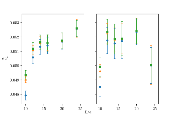
Figure 8: Values of the time-like $\sigma_{t}a^{2}$ (left panel) and space-like $\sigma_{s}a^{2}$ (right panel) string tensions extracted at fixed lattice spacing ($\beta=7.7$) and varying lattice size $L/a$, using the LO($\bullet$), NLO($\blacktriangle$) and NG($\blacksquare$) expressions for the ground state energies from Eqs. (77), (78) and (79), respectively.

Our final estimate for the value of $\sqrt{\sigma}$ as a function of $L$ is obtained from the first two columns of Table 3 by computing the weighted average

$$\sqrt{\sigma} = \frac{\frac{\sqrt{\sigma_{t}}}{(\Delta\sqrt{\sigma_{t}})^{2}}+\frac{\sqrt{\sigma_{s}}}{(\Delta\sqrt{\sigma_{s}})^{2}}}{\left(\frac{1}{\Delta\sqrt{\sigma}}\right)^{2}}\,,$$ (90)

where the error is given by

$$\Delta\sqrt{\sigma} =\frac{1}{\sqrt{\frac{1}{(\Delta\sqrt{\sigma_{t}})^{2}}+\frac{1}{(\Delta\sqrt{\sigma_{s}})^{2}}}}\,.$$

The resulting values are reported in the last column. From the behaviour of $\sqrt{\sigma}$ we conclude that finite size effects are certainly smaller than the statistical error for $L\geq 14a$, and we take as a final estimate of $\sqrt{\sigma}$ at this coupling the value at $L=16a$. We also note that compatible results are obtained for $L=12a$.

Assuming scaling towards the continuum, from our finite-size study we obtain firm evidence that all lattices for which $L\sqrt{\sigma}\geq 3$ provide an estimate of the string tension that is compatible within the statistical errors with the infinite-volume value. Hence, we conclude that finite-volume effects are negligible once $L\sqrt{\sigma}\mathrel{\raisebox{-2.58334pt}{$\stackrel{{\scriptstyle\textstyle>}}{{\sim}}$}}3$. In particular, we have verified that the condition $L\sqrt{\sigma}\mathrel{\raisebox{-2.58334pt}{$\stackrel{{\scriptstyle\textstyle>}}{{\sim}}$}}3$ is safely fulfilled when carrying out calculations on lattice ensembles with larger $\beta$, starting from the finite-size analysis at $\beta=7.7$. Table 2 reports the lattice parameters of the calculations we have used to extrapolate to the continuum limit and the corresponding results for $\sqrt{\sigma}$.

5.3.2 The mass spectrum of glueballs

As for the string tension, we began our analysis of glueball masses with a study of finite-size effects for lattice coupling $\beta=7.7$. We aimed at estimating finite-volume effects as a function of the lattice size $L$, and bound $L$ such that the systematic error due to the finite size be negligible with respect to statistical error on the measurement of the masses.

Our results for the mass spectrum at $\beta=7.7$ for various volumes are reported in the rows of Table 4. While this particular choice of $\beta$ is suitable for finite-size studies, as it allows us to reach large lattices in physical units with a relatively small computational effort, the coarseness of the lattice spacing pushes most of the masses above the lattice cut-off, making their extraction numerically challenging. For this reason, we observe a systematic effect related to the isolation of the ground state on all irreducible representations other than the lowest-lying one. While in our tables we quote only the statistical error, for higher excitations the systematic error coming from the ground state isolation in a given channel is expected to have a comparable size.

Another systematic effect that affects our calculation of the glueball masses is contamination of the spectrum by multi-glueball scattering states and torelon states (the latter being lattice artefacts associated with state propagation of pairs of oppositely directed Polyakov loops). Separating the physical spectrum from those unwanted states requires a more demanding calculation that goes beyond the scope of this first exploration of the glueball masses in $Sp(4)$. What results is a hard-to-control error related to mixing with spurious states, which is strongly dependent on the volume and manifests itself in occasional sudden jumps and irregularities of the extracted masses. Indeed this is visible for some of the most massive states we report in Table 4. In view of all these considerations, and to focus the discussion to the main purposes of this paper, we limit the analysis of finite-size effects at $\beta=7.7$ to the ground state (found in the $A1^{+}$ channel) and to the would-be continuum $2^{+}$ glueball (expected to appear in the $E^{+}$ and in the $T1^{+}$ channels).

$R^{P}$	$L/a=10$	$L/a=12$	$L/a=14$	$L/a=16$	$L/a=20$	$L/a=24$
$A1^{+}$	$0.569(13)$	$0.728(15)$	$0.738(16)$	$0.742(16)$	$0.764(15)$	$0.739(11)$
$A1^{-}$	$1.039(35)$	$1.275(41)$	$1.406(47)$	$1.210(40)$	$1.300(34)$	$1.323(34)$
$A2^{+}$	$1.70(11)$	$1.706(95)$	$1.778(95)$	$1.650(76)$	$1.771(81)$	$1.748(74)$
$A2^{-}$	$2.48(34)$	$1.83(17)$	$1.74(14)$	$2.21(25)$	$2.23(24)$	$2.252(22)$
$E^{+}$	$0.623(13)$	$1.111(32)$	$1.150(32)$	$1.159(27)$	$1.217(26)$	$1.036(59)$
$E^{-}$	$1.402(62)$	$1.347(58)$	$1.401(48)$	$1.509(66)$	$1.597(59)$	$1.463(45)$
$T1^{+}$	$1.170(43)$	$1.220(36)$	$1.202(39)$	$1.209(31)$	$1.173(26)$	$1.82(11)$
$T1^{-}$	$1.465(75)$	$1.513(69)$	$1.515(66)$	$1.522(57)$	$1.499(51)$	$1.87(12)$
$T2^{+}$	$1.53(11)$	$1.70(12)$	$1.99(14)$	$1.578(94)$	$1.839(96)$	$1.179(95)$
$T2^{-}$	$1.60(12)$	$2.04(18)$	$2.38(27)$	$2.07(18)$	$1.94(15)$	$1.505(46)$

Table 4: Glueball masses obtained at coupling $\beta=7.7$, with operators blocked at level $N_{b}\leq N_{L}$ and with $15$ cooling steps. The quantum number $R^{P}$ refer to the octahedral group as explained in Sec. 5.1. The calculations are repeated for various values of the lattice size $L/a$.

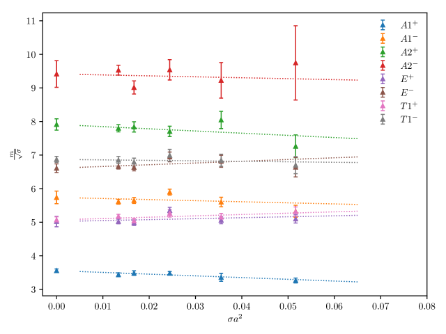
Figure 9: Continuum limit extrapolations of the glueball masses $m/\sqrt{\sigma}$, in units of the string tension, in $Sp(4)$ Yang-Mills, as described in Sec. 5.3.2. States are labelled by the quantum numbers of the octahedral group, but notice the emergence of degeneracies in the continuum limit, in the case of $T_{1}^{+}$ and $E^{+}$, as well as $T_{1}^{-}$ and $E^{-}$.

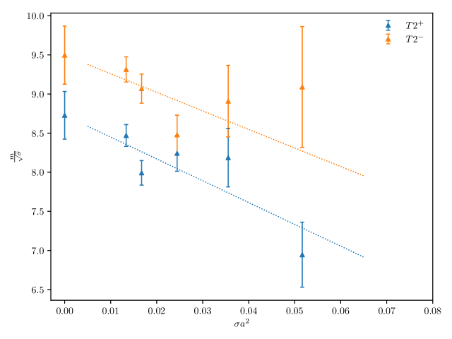
Figure 10: Continuum limit extrapolations of the glueball masses $m/\sqrt{\sigma}$, in units of the string tension, in $Sp(4)$ Yang-Mills, as described in Sec. 5.3.2. States are labelled by the quantum numbers of the octahedral group.

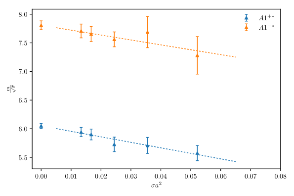
Figure 11: Continuum limit extrapolations of the glueball masses for selected excited states $m/\sqrt{\sigma}$, in units of the string tension, in $Sp(4)$ Yang-Mills, as described in Sec. 5.3.2. States are labelled by the quantum numbers of the octahedral group.

$R^{P}$	$m(R^{P})/\sqrt{\sigma}$
$A1^{+}$	$3.557(52)$
$A1^{+*}$	$6.05(4)$
$A1^{-}$	$5.74(19)$
$A1^{-*}$	$7.81(8)$
$A2^{+}$	$7.91(17)$
$A2^{-}$	$9.42(40)$
$E^{+}$	$5.02(16)$
$E^{-}$	$6.61(13)$
$T1^{+}$	$5.070(91)$
$T1^{-}$	$6.872(89)$
$T2^{+}$	$8.73(30)$
$T2^{-}$	$9.50(37)$

Table 5: Continuum extrapolated glueball masses in all the symmetry channels. States are labelled by the quantum numbers of the octahedral group.

Starting with the $A1^{+}$ state, we fit the behaviour of the extracted mass to the size dependency parameterised as follows:

$$m(L)=m\left(1+\frac{b_{1}e^{-b_{2}mL}}{mL}\right)\,,$$ (91)

and we find its infinite volume limit to be

$$am=0.746(6)\ ,\qquad\chi^{2}/{\rm d.o.f}=0.68\ .$$ (92)

This value for $am$ is compatible within errors with all the measured masses in the $A1^{+}$ channel for $L/a\geq 12$. Hence, as in the case of the string tension discussed earlier, the systematic error due to neglecting the finite size of the lattice is found to be comfortably less than the statistical error as long as $L\sqrt{\sigma}\geq 3$. Thus, having taken care that this bound be satisfied at all $\beta$ values simulated for the continuum extrapolation, in the extraction of the continuum limit we shall use the value measured at one lattice size.

It is also interesting to look at the masses in the $E^{+}$ and in the $T1^{+}$ channels, as the lowest-lying states in these two channels are expected to be degenerate in the continuum limit, since they correspond to different polarisations of the continuum $2^{+}$ state. From Table 4 we infer that this degeneracy is satisfied for lattice sizes other than the smallest $L/a=10$ (for which large finite-size effects are expected to arise differently in the two channels) and the largest $L/a=24$, where some uncontrolled systematics (possibly due to mixing with spurious states) creates visible anomalies in this measurement. We take the agreement in the intermediate region as a good indication that $\beta=7.7$ is sufficiently close to the continuum limit to justify its inclusion in the continuum extrapolation.

Going towards the continuum, we have measured glueball masses in the various lattice channels for the couplings and volumes reported in the first two columns of Table 2. Continuum extrapolations for the ratio $m_{G}/\sqrt{\sigma}$ are obtained from the expectation that the corrections due to discretisation are linear in $\sigma a^{2}$. The results are reported in Table 5.3.2 and represented in Figs. 9 and 10. Some excited states are shown in Fig. 11. As expected, in the continuum limit the states $T_{1}^{\pm}$ and $E^{\pm}$ are degenerate in pairs. The channels $T_{2}^{\pm}$ show strong fluctuations and discretisation effects that are caused by the difficulty in extracting their masses in lattice units. The values obtained for the $0^{+}$ and $2^{+}$ states are at the same order of magnitude as those obtained in $SU(N)$ theories Lucini:2001ej .

5.3.3 Epilogue

In this Section, we have reported on what is (to the best of our knowledge) the first controlled calculation in the continuum limit of the glueball spectrum and of the string tension for the $Sp(4)$ pure Yang-Mills theory. The main purpose of our study is to gain some understanding of the glue dynamics in this theory, and progressively aim at providing an interpretation of the results emerging from the theory with dynamical quarks. Nevertheless, the outcomes of our investigation in the pure gauge case are interesting in their own right: for instance, they provide a first step towards a systematic calculation of the pure Yang-Mills spectrum in the large $N$ limit of $Sp(2N)$ gauge theories and give us an opportunity to contrast the non-perturbative dynamics of $Sp(2N)$ with that of $SU(N)$ gauge theories.

Albeit expected, the first remarkable outcome of our calculation is that the pure gauge quantities behave not dissimilarly from those of $SU(N)$. The mass associated to the decay of Polyakov-loop correlators follows the properties expected from a confining flux tube, hence supporting the confining nature of the pure gauge dynamics in $Sp(4)$. The lowest-lying state in the glueball spectrum is the $0^{+}$ glueball. The ratio $m_{0^{+}}/\sqrt{\sigma}\simeq 3.55$ is not far from the large-$N$ value from $SU(N)$ groups, $m_{0^{++}}/\sqrt{\sigma}\simeq 3.3$ Lucini:2012gg , and is indeed compatible within errors with the $SU(3)$ value of $m_{0^{++}}/\sqrt{\sigma}=3.55(7)$ Lucini:2004my , with the value for $SU(4)$ of $m_{0^{++}}/\sqrt{\sigma}=3.36(6)$ being appreciably different, albeit close.

This behaviour is consistent with the above ratio being a mildly decreasing function of the number of generators—while $SU(4)$ has 15 generators, $SU(3)$ has 8 and $Sp(4)$ has 10— and deserves further enquiry by performing numerical studies of $Sp(2N)$ gauge theories at larger $N$. An interesting observation has been put forward in Hong:2017suj , by suggesting that

$$\frac{m_{0^{++}}^{2}}{\sigma}=\eta\frac{C_{2}(A)}{C_{2}(F)}\ ,$$ (93)

where $C_{2}(A)$ and $C_{2}(F)$ are the quadratic Casimir of the adjoint and of the fundamental representation, respectively, and $\eta$ is a universal constant, in the sense that it depends on the dimensionality of the spacetime, but not on the gauge group. Noting that for $Sp(2N)$

$$\frac{C_{2}(A)}{C_{2}(F)}=\frac{4\left(N+1\right)}{2N+1}\ ,$$ (94)

we find that our determination of the proportionality constant

$$\eta=5.27(15)\ ,$$ (95)

is compatible with the value $\eta=5.41(12)$ extracted from $SU(N)$ in 3+1 dimensions Hong:2017suj .

The rest of the glueball spectrum also follows a pattern that is broadly similar to that of $SU(N)$. Another interesting quantity in the glueball sector is the ratio $m_{2^{++}}/m_{0^{++}}$. Using universality arguments, it has been argued in Athenodorou:2016ndx that for confining theories where the dynamics does not yield large anomalous dimensions, as in pure Yang-Mills, one should find $m_{2^{++}}/m_{0^{++}}=\sqrt{2}$. Our numerical results give $m_{2^{++}}/m_{0^{++}}=1.425(32)$, a value that is fully compatible with the conjecture of Athenodorou:2016ndx .

Besides being relevant for models of electroweak symmetry breaking based on a Pseudo-Nambu-Goldstone interpretation of the Higgs field, the investigation of which is the central leitmotif of this paper, studies of $Sp(2N)$ pure gauge theories provide new relevant information on universal aspects of Yang-Mills dynamics. We shall develop this latter line of research in future numerical investigations.

6 Of quenched mesons: masses and decay constants

In this Section, we present our results for the masses and decay constants of the lightest flavoured mesons in the quenched approximation. Our main purpose is to illustrate the process that we envision we will carry out once simulations with dynamical quarks are available. Although we are aware of the fact that the quenched results may not capture in full the features of the theory, we still expect it to provide some useful information about its qualitative features. Experience on QCD with light quarks suggests that several quantities are well captured by the quenched approximation, although we already cautioned the reader about the fact that such considerations may not extend to these dynamical theories.

The EFT in Sec. 2.1, within the limitations discussed therein, describes the continuum limit of the dynamical simulations, not the quenched ones. In principle, one could make more sense of the comparison by adopting the approach of quenched chiral perturbation theory Bernard:1992mk ; Sharpe:1992ft or of partially-quenched chiral perturbation theory Sharpe:2000bc ; Sharpe:2001fh ; Bernard:1993sv , but for present purposes our strategy will suffice, though we invite the reader to use caution, in particular for quantities such as the $g_{\rho\pi\pi}$ coupling, that are certainly affected by the quenching procedure.

6.1 Observables

As discussed in Sec. 2.1, the observables of most direct phenomenological relevance, and at the same time the most directly accessible to lattice calculations, are the masses, $m_{M}$, and the decay constants, $f_{M}$, of pseudo-scalar, vector and axial-vector mesons. This numerical study focuses on flavoured particles. The interpolating operators and quantum numbers are summarised in Table 6.

Label	Operator ${\cal O}_{M}$	Meson	$J^{P}$
$PS$	$\overline{Q^{i}}\gamma_{5}Q^{j}$	$\pi$	$0^{-}$
$V$	$\overline{Q^{i}}\gamma_{\mu}Q^{j}$	$\rho$	$1^{-}$
$AV$	$\overline{Q^{i}}\gamma_{5}\gamma_{\mu}Q^{j}$	$a_{1}$	$1^{+}$

Table 6: Interpolating operators used for the measurement of the properties of flavoured mesons ($i\neq j$) in the pseudo-scalar (PS), vector (V) and axial-vector (AV) cases, associated with the $\pi$, $\rho$ and $a_{1}$ mesons, respectively. We also report the Lorentz-group quantum numbers $J^{P}$. The summations over colour and spinor indices are understood.

We define the ensemble average of two-point meson correlators in the Euclidean space as

$$C_{\mathcal{O}_{M}}(\vec{p},t) \equiv \sum_{\vec{x}}e^{-i\vec{p}\cdot\vec{x}}\langle 0|\mathcal{O}_{M}(\vec{x},t)\mathcal{O}_{M}^{\dagger}(\vec{0},0)|0\rangle\,,$$ (96)

where $\mathcal{O}_{M}$ denotes any of the meson interpolating operators in Table 6. In the limit in which the Euclidean time $t$ is large, and for vanishing three-momentum $\vec{p}$, the correlation function is dominated by the ground state. Its exponential decay is controlled by the meson mass $m_{M}$, and can be approximated as

$$C_{\mathcal{O}_{M}}(t)\xrightarrow{t\rightarrow\infty}\langle 0|\mathcal{O}_{M}|M\rangle\langle 0|\mathcal{O}_{M}|M\rangle^{*}\frac{1}{m_{M}L^{3}}\left[e^{-m_{M}t}+e^{-m_{M}(T-t)}\right]\,,$$ (97)

where $T$ and $L$ are the temporal and the spatial extent of the lattice, respectively. In the meson states $|M\rangle$, we define $M=M^{i}T^{i}$, with $T^{i}$ the generators of the group. Using this convention, the mesonic matrix elements are parameterised in terms of decay constants $f_{M}$ and masses $m_{M}$ as

$$\langle 0|\overline{Q_{1}}\gamma_{5}\gamma_{\mu}Q_{2}|PS\rangle = f_{\pi}p_{\mu}\,,$$

$$\langle 0|\overline{Q_{1}}\gamma_{\mu}Q_{2}|V\rangle = f_{\rho}m_{\rho}\epsilon_{\mu}\,,$$

$$\langle 0|\overline{Q_{1}}\gamma_{5}\gamma_{\mu}Q_{2}|AV\rangle = f_{a_{1}}m_{a_{1}}\epsilon_{\mu}\,,$$ (98)

where $\epsilon_{\mu}$ is the polarisation vector obeying $\epsilon_{\mu}p^{\mu}=0$ and $\epsilon_{\mu}\epsilon^{\mu}=+1$. Using Eq. (97) and Eq. (98), for vector and axial-vector mesons we can rewrite the correlation functions

$$C_{\mathcal{O}_{V}}(t) \xrightarrow{t\rightarrow\infty} \frac{m_{\rho}f_{\rho}^{2}}{L^{3}}\left[e^{-m_{\rho}t}+e^{-m_{\rho}(T-t)}\right],$$

$$C_{\mathcal{O}_{AV}}(t) \xrightarrow{t\rightarrow\infty} \frac{m_{a_{1}}f_{a_{1}}^{2}}{L^{3}}\left[e^{-m_{a_{1}}t}+e^{-m_{a_{1}}(T-t)}\right].$$ (99)

To calculate the decay constant of the pseudo-scalar meson, we additionally consider the following two-point correlation function

$$C_{\Pi}(\vec{p},t) = \sum_{\vec{x}}e^{-i\vec{p}\cdot\vec{x}}\langle 0|[\overline{Q_{1}}\gamma_{5}\gamma_{\mu}Q_{2}(\vec{x},t)]\,[\overline{Q_{1}}\gamma_{5}Q_{2}(\vec{0},0)]|0\rangle$$ (100)

$$\xrightarrow{t\rightarrow\infty} \frac{f_{\pi}\langle 0|\mathcal{O}_{PS}|PS\rangle^{*}}{L^{3}}\left[e^{-m_{\pi}t}-e^{-m_{\pi}(T-t)}\right].$$

The pion mass $m_{\pi}$ and matrix element $\langle 0|\mathcal{O}_{PS}|PS\rangle$ are obtained from the pion correlator,

$$C_{\mathcal{O}_{PS}}(t) \xrightarrow{t\rightarrow\infty} \frac{|\langle 0|\mathcal{O}_{PS}|PS\rangle|^{2}}{m_{\pi}L^{3}}\left[e^{-m_{\pi}t}+e^{-m_{\pi}(T-t)}\right].$$ (101)

Meson decay constants computed on the lattice are matched to the continuum. In this work, we perform one-loop matching in lattice perturbation theory. Because we are using Wilson fermions, the axial and vector currents are not conserved in the lattice theory, and hence receive (finite) renormalization, that we write as

$$f^{\rm ren}_{\pi}=Z_{A}f_{\pi}\,,~{}~{}~{}f^{\rm ren}_{\rho}=Z_{V}f_{\rho}\,,~{}~{}~{}{\rm and}~{}~{}~{}f^{\rm ren}_{a_{1}}=Z_{A}f_{a_{1}}\,.$$ (102)

The pion decay constant $f_{\pi}$ is renormalised by $Z_{A}$, as the axial current is used to define $f_{\pi}$ in Eq. (98). In the continuum limit, the renormalization constants are expected to be unity. The one-loop matching coefficients taken from Martinelli:1982mw are given by

$$Z_{A} = 1+C(F)\left(\Delta_{\Sigma_{1}}+\Delta_{\gamma_{5}\gamma_{\mu}}\right)\frac{g^{2}}{16\pi^{2}}\,,$$

$$Z_{V} = 1+C(F)\left(\Delta_{\Sigma_{1}}+\Delta_{\gamma_{\mu}}\right)\frac{g^{2}}{16\pi^{2}}\,,$$ (103)

where $g$ is the coupling constant and the eigenvalue of the quadratic Casimir operator is $C(F)=5/4$ for $Sp(4)$. The coefficients $\Delta_{I}$, relating the lattice computation with the continuum $\overline{\rm MS}$ regularisation scheme, result from one-loop integrals performed numerically, and are summarised in Table 7. We notice that the coefficients reported here have been obtained by restricting the integrals within the first Brillouin zone. We verified explicitly that the errors in numerical evaluation for these integrals are $2\%$ or less, and that there are no discernible finite-volume effects. Therefore we neglect the uncertainty on the $\Delta_{i}$ coefficients in the rest of this paper. The coefficient $\Delta_{\Sigma_{1}}$ is taken from the wave-function renormalization of the external fermion lines, without taking into account the power-divergence contribution, while the coefficients $\Delta_{\gamma_{\mu}}$ and $\Delta_{\gamma_{5}\gamma_{\mu}}$ are extracted from the one-loop computations of the vertex functions.

$\Delta_{\Sigma_{1}}$	$\Delta_{\gamma_{\mu}}$	$\Delta_{\gamma_{5}\gamma_{\mu}}$
$-12.82$	$-7.75$	$-3.00$

Table 7: Results of one-loop integrals for the matching coefficients in Eq. (103) at the choice of the Wilson parameter $r=1$, and taken from Martinelli:1982mw .

Wilson fermions receive quite large renormalisation and thus the perturbative expansion with the bare coupling is reliable only at very large values of the lattice coupling $\beta=4N/g^{2}$. As in the continuum case, in lattice perturbation theory, the appropriate expansion parameter is the renormalised coupling $\bar{g}$ rather than the bare counterpart $g$. Following Lepage:1992xa , we use the simple tadpole improved coupling defined by

$$\bar{g}^{2} \equiv \frac{2Ng^{2}}{\langle{{\rm Tr\,}}\,\mathcal{P}\rangle}\,,$$ (104)

where $\mathcal{P}$ is the plaquette operator.

6.2 Numerical results and EFT

$\beta$	$~{}a^{2}t_{0}^{p}~{}$	$~{}a^{2}t_{0}^{c}~{}$	$~{}aw_{0}^{p}~{}$	$~{}aw_{0}^{c}~{}$	$\langle P\rangle$	$~{}~{}Z_{V}~{}~{}$	$~{}~{}Z_{A}~{}~{}$
$7.62$	$1.805(7)$	$2.049(7)$	$1.436(4)$	$1.448(4)$	$0.60190(19)$	$0.71599(9)$	$0.78157(7)$
$8.0$	$4.899(18)$	$5.115(19)$	$2.300(6)$	$2.308(6)$	$0.63074(13)$	$0.74185(5)$	$0.80146(4)$

Table 8: Gradient-flow scales $t_{0}^{p}$, $t_{0}^{c}$, $w_{0}^{p}$ and $w_{0}^{c}$, plaquette values $\langle P\rangle$, and one-loop matching factors $Z_{V}$ and $Z_{A}$, computed for the two values of the lattice coupling $\beta$ used in subsequent exploratory quenched calculations. The errors quoted arise from the stochastic determination of the tadpole-improved coupling.

As a first exploratory step towards understanding the qualitative features of mesons of the $Sp(4)$ theory, as well as to test the low-energy EFT and illustrate its use, we calculate the mesonic observables described in the previous section in the quenched approximation at $\beta=7.62$ and $8.0$. For each ensemble we generate $200$ gauge configurations on a lattice of size $48\times 24^{3}$, using the HB algorithm. We first measure the plaquette values (which are used to compute the one-loop matching factors in Eq. (103) with the tadpole improved coupling $\bar{g}$), and the gradient flow scales $t_{0}$ and $w_{0}$. The numerical results are summarised in Table 8. The gradient flow scales are determined by setting $\mathcal{E}_{0}=\mathcal{W}_{0}=0.35$. As discussed in Section 4, we use two definitions of $G_{\mu\nu}$ denoted by the superscript $p$ for a plaquette and $c$ for a (four-plaquette) clover, with the difference of the two measuring the size of finite lattice spacing artefacts. We find that, compared to $t_{0}$, the difference between the clover and the plaquette regularisations for $w_{0}$ is significantly smaller, and thus we choose to use $w_{0}^{c}$ to convert lattice units to physical ones.

$am_{0}$	$a^{2}m_{\pi}^{2}$	$a^{2}m_{\rho}^{2}$	$a^{2}m_{a_{1}}^{2}$	$a^{2}f_{\pi}^{2}$	$a^{2}f_{\rho}^{2}$	$a^{2}f_{a_{1}}^{2}$
$-0.65$	0.4325(5)	0.5087(8)	1.04(4)	0.01451(9)	0.0376(3)	0.021(4)
$-0.7$	0.3042(4)	0.3916(11)	0.943(29)	0.01246(8)	0.0365(4)	0.029(3)
$-0.73$	0.2318(4)	0.3272(14)	0.862(20)	0.01101(8)	0.0354(5)	0.0313(20)
$-0.75$	0.1856(4)	0.2875(15)	0.831(16)	0.00995(8)	0.0346(4)	0.0352(16)
$-0.77$	0.1409(4)	0.2485(19)	0.769(22)	0.00879(8)	0.0329(6)	0.0350(22)
$-0.78$	0.1191(4)	0.2312(21)	0.796(17)	0.00822(8)	0.0327(6)	0.0415(16)
$-0.79$	0.0977(4)	0.2115(26)	0.772(20)	0.00760(8)	0.0314(8)	0.0418(19)
$-0.8$	0.0765(4)	0.193(3)	0.748(24)	0.00698(8)	0.0301(10)	0.0417(23)
$-0.81$	0.0553(4)	0.175(5)	0.73(3)	0.00635(9)	0.0285(14)	0.042(3)
$-0.815$	0.0446(4)	0.166(7)	0.70(4)	0.00606(9)	0.0280(19)	0.040(4)
$-0.82$	0.0328(4)	0.158(13)	0.70(6)	0.00572(15)	0.028(4)	0.041(6)

Table 9: Masses and decay constants (squared) of pseudo-scalar ($\pi$), vector ($\rho$), and axial-vector ($a_{1}$) mesons, as obtained from the quenched calculations described in Sec. 6.2, for $\beta=7.62$ on lattice of size $48\times 24^{3}$.

$am_{0}$	$a^{2}m_{\pi}^{2}$	$a^{2}m_{\rho}^{2}$	$a^{2}m_{a1}^{2}$	$a^{2}f_{\pi}^{2}$	$a^{2}f_{\rho}^{2}$	$a^{2}f_{a_{1}}^{2}$
$-0.45$	0.5556(12)	0.5837(13)	0.868(13)	0.00832(14)	0.0153(3)	0.0057(5)
$-0.5$	0.4244(11)	0.4551(14)	0.734(11)	0.00771(14)	0.0149(3)	0.0073(6)
$-0.55$	0.3037(8)	0.3383(12)	0.593(11)	0.00691(10)	0.0145(3)	0.0084(7)
$-0.6$	0.1937(8)	0.2325(14)	0.465(12)	0.00567(8)	0.0131(3)	0.0096(8)
$-0.625$	0.1437(7)	0.1862(16)	0.405(13)	0.00494(8)	0.0125(4)	0.0102(10)
$-0.64$	0.1156(7)	0.1612(15)	0.363(20)	0.00449(7)	0.0124(3)	0.0099(18)
$-0.65$	0.0974(7)	0.1448(16)	0.349(15)	0.00414(7)	0.0120(3)	0.0109(13)
$-0.66$	0.0812(5)	0.1302(14)	0.343(14)	0.00397(5)	0.0123(3)	0.0128(12)
$-0.67$	0.0642(5)	0.1179(18)	0.318(18)	0.00352(4)	0.0123(4)	0.0123(17)
$-0.68$	0.0479(4)	0.1040(22)	0.323(13)	0.00319(4)	0.0122(5)	0.0150(11)
$-0.69$	0.0318(4)	0.0907(28)	0.304(19)	0.00270(5)	0.0115(5)	0.0151(17)

Table 10: Masses and decay constants (squared) of pseudo-scalar ($\pi$), vector ($\rho$), and axial-vector ($a_{1}$) mesons, as obtained from the quenched calculations described in Sec. 6.2, for $\beta=8.0$ on lattice of size $48\times 24^{3}$.

The mesonic two-point correlation functions in Eq. (96) are measured using stochastic wall sources Boyle:2008rh at various quark masses. While at sufficiently large time we use the asymptotic expressions of two-point correlation functions in Eqs. (97), (99) and (100) to extract the meson masses and decay constants, we perform multi-exponential fits when the time extent is not large enough to reach the asymptotic region, according to

$$C_{\mathcal{O}_{M}}(t)=\sum_{i=0}^{\infty}C_{i}\left(e^{-E_{i}t}+e^{-E_{i}(N_{t}-t)}\right)\,,$$ (105)

where $E_{0}=m_{M}<E_{1}<E_{2}<\cdots$. We find that the two-exponential fits are good enough to describe the numerical data in most cases. The numerical results (not renormalised) are summarised in Tables 9 and 10. The statistical errors are estimated by using a standard bootstrapping technique (with about 250 bootstrap samples) and a correlated fit with $\chi^{2}$ minimisation.

	fit range ($m_{0}$)	$~{}~{}~{}\chi^{2}/{\rm d.o.f}~{}~{}~{}$	$~{}~{}~{}~{}~{}w_{0}^{c}~{}m_{0}^{*}~{}~{}~{}~{}~{}$	$~{}~{}~{}~{}~{}w_{0}^{c}v~{}~{}~{}~{}~{}$	$~{}~{}~{}~{}~{}w_{0}^{c}v_{5}~{}~{}~{}~{}~{}$
$\beta=7.62$	$[-0.82,\,-0.73]$	$0.17$	$-1.214(22)$	$0.750(5)$	$0.408(5)$
$\beta=8.0$	$[-0.69,\,-0.625]$	$0.58$	$-1.636(27)$	$0.862(27)$	$0.431(22)$

Table 11: Results of the fit of the quenched meson data to the GMOR relation in Eq. (35), where the quark mass $m$ is replaced by the combination $w_{0}^{c}(m_{0}-m_{0}^{*})$.

	fit range ($m_{0}$)	$~{}~{}~{}\chi^{2}/{\rm d.o.f}~{}~{}~{}$	$~{}~{}~{}~{}~{}w_{0}^{c}\bar{v}~{}~{}~{}~{}~{}$	$~{}~{}~{}~{}~{}w_{0}^{c}\bar{v}_{5}~{}~{}~{}~{}~{}$
$\beta=7.62$	$[-0.82,\,-0.75]$	$0.19$	$0.1839(17)$	$0.1302(16)$
$\beta=8.0$	$[-0.69,\,-0.66]$	$0.74$	$0.1873(25)$	$0.1276(34)$

Table 12: Results of the fit of the quenched meson data to the GMOR relation in Eq. (35), where the quark mass $m$ is replaced by the combination $(w_{0}^{c}m_{\rm PS})^{2}$. The barred variables are defined as $\bar{v}=v/(2B)^{1/3}$ and $\bar{v}_{5}=v_{5}/(2B)$.

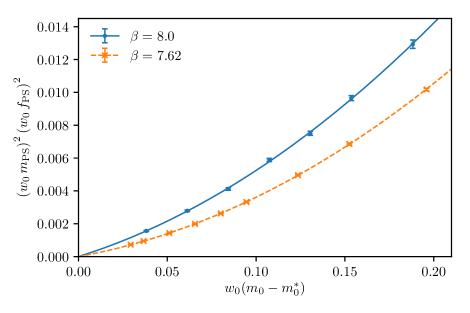
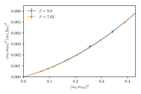
Figure 12: Tests of the GMOR relation in the quenched data. The solid and dashed lines are fit results for the cases of $\beta=8.0$ and $7.62$, respectively. In the top panel, we show the result of identifying the quark mass with the quantity $w_{0}(m_{0}-m_{0}^{*})$, replaced in the lower panel by $(w_{0}m_{\rm PS})^{2}$.

To analyse the numerical results using the continuum EFT developed in Sec. 2.1, we reinstate the correct dimensionality by expressing all mass and decay constants in units of $w_{0}=w_{0}^{c}$. The decay constants are further renormalised using perturbative one-loop matching.

Let us first restrict our attention to the pseudo-scalar mesons and check the GMOR relation. In the upper panel of Fig. 12 we plot $m_{PS}^{2}f_{PS}^{2}$, against the quark mass, where the latter is defined by the difference between the bare quark mass and the critical mass at which the mass of pseudo-scalar mesons vanishes. Even for the lightest masses $m_{0}$ available we do not find the expected leading-order linear behaviour. Therefore, we fit the data to the NLO results including the $v_{5}$ term in Eq. (2.1.2). The solid and dashed lines in Fig. 12 are the fit results for $\beta=8.0$ and $7.62$, respectively, where the fitting ranges and the resulting fit parameters are found in Table 11.

As the quark mass is scheme-dependent, to compare the lattice results obtained with different coupling we would have to properly renormalise the quark mass. Instead of doing so, we consider the GMOR relation with respect to the pseudo-scalar meson mass, $m_{PS}$, which is a scheme independent (physical) quantity, and show the result in the bottom panel of Fig. 12. As shown in the fit results in Tab. 12, we find that the parameters of the NLO GMOR relation between two lattices are statistically consistent, implying that finite lattice artefacts affect this observable only in a negligible way.

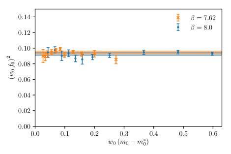
Figure 13: The quantity $f_{0}^{2}=f_{\pi}^{2}(0)+f_{\rho}^{2}+f_{a_{1}}^{2}$, defined in Eq. (22), measured in the quenched approximation for varying values of $w_{0}(m_{0}-m_{0}^{*})$.

One of the interesting quantities in the EFT is $f_{0}^{2}$, the sum of the squared decay constants of pseudo-scalar, vector, and axial-vector mesons, which is independent of the mass $m_{0}$ if one adopts Eq. (2.1.2). As shown in Fig. 13, the numerical results are in good agreement with such expectation. In the figure, blue circles and orange crosses represent the choices $\beta=7.62$ and for $\beta=8.0$, respectively. Notice that we derived this relation from our NLO EFT at the tree level. In principle, one has to consider the contribution from the one-loop corrections, including chiral logarithms. We performed a constant fit to the results and obtained $f_{0}^{2}(\beta=8.0)=0.0926(17)$ and $f_{0}^{2}(\beta=7.62)=0.0944(18)$ denoted by blue and orange bands, respectively. As for the case of the GMOR relation, we find that lattice spacing artefacts in $f_{0}^{2}$ are negligible, in the sense that no appreciable difference is measured.

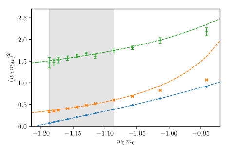
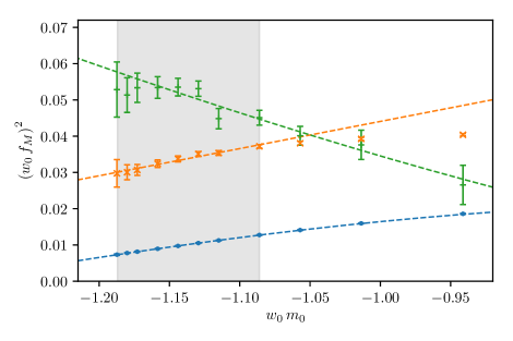
Figure 14: Plots of the meson masses (top panel) and decay constants (bottom panel) from the quenched calculation with $\beta=7.62$, compared to the best-fit results based upon the EFT description in Sec. 2.1.2. Blue circles, orange crosses, and green bars represent for pseudo-scalar ($\pi$), vector ($\rho$), and axial-vector ($a_{1}$) mesons, respectively. For the EFT fits are based on the data in the shaded region.

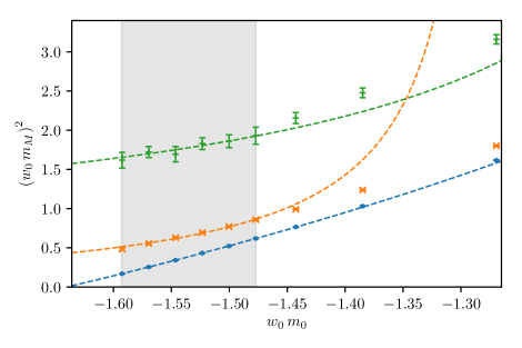
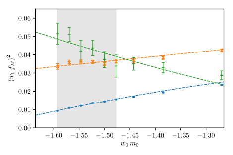
Figure 15: Plots of the meson masses (top panel) and decay constants (bottom panel) from the quenched calculation with $\beta=8.0$, compared to the best-fit results based upon the EFT description in Sec. 2.1.2. Blue circles, orange crosses, and green bars represent for pseudo-scalar ($\pi$), vector ($\rho$), and axial-vector ($a_{1}$) mesons, respectively. For the EFT fits are based on the data in the shaded region.

We finally use the NLO EFT relations to construct a global fit to the meson masses and decay constants. The results are illustrated in Figs. 14 and 15. We perform an uncorrelated fit to the data, restricted to the eight and six lightest masses $m_{0}$ for $\beta=7.62$ and $8.0$, respectively. The fitting range is shown as the shaded region in the figures. There are two main technical difficulties in this fit procedure. First of all, the parameter space is too large to determine the actual global minimum. In the NLO EFT we have thirteen fit parameters (including the critical bare mass $m_{0}^{\ast}$). The standard $\chi^{2}$ minimisation is not stable, and it typically yields two qualitatively very different results, one fairly linear and one exhibiting highly nonlinear behaviours with respect to the quark mass. We take the former as our best fit as the stability of the fits is better than the latter when we vary the fitting range. Secondly, statistical uncertainties vary widely for different types of mesons, and as a result the pseudo-scalar mesons tightly constrain the fit results. Furthermore, the numerical data suffer from several systematics such as quenching and discretising effects.

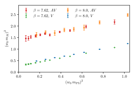
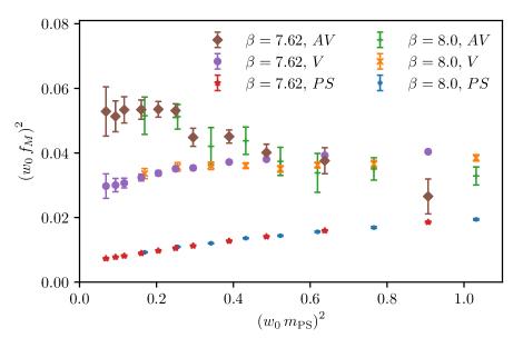
Figure 16: Comparison between the meson masses (top panel) and decay constants (bottom panel) in the quenched calculations with two different values of the lattice coupling $\beta$. The colour coding for the pseudo-scalar, vector, and axial-vector mesons is explained by the legend. The numerical results are shown as a function of the combination $(w_{0}m_{\rm PS})^{2}$, highlighting the corresponding reduction of finite-spacing effects.

Undeterred by all these limitations and difficulties, since the purpose of this explorative study with quenched calculations is to show how our EFT works, we attempted to perform the global fit to the central values using the standard $\chi^{2}$ minimisation. The fit results are represented by the dashed lines in the figures. For completeness, we report the resulting values of the fit parameters for $\beta=7.62$:

$$\kappa=-0.83,~{}y_{3}/w_{0}=-0.41,~{}y_{4}/w_{0}=3.14,~{}g_{\rho}=1.93,~{}b=-0.38,~{}c=0.027,$$

$$~{}fw_{0}=0.84,Fw_{0}=0.57,~{}v_{1}w_{0}=0.075,~{}v_{2}w_{0}=-0.33,~{}vw_{0}=0.27,~{}v_{5}w_{0}=0.40,$$

$$~{}m_{0}^{*}w_{0}=-1.21,~{}\chi^{2}/{\textrm{d.o.f}}=0.11\,,$$

and for $\beta=8.0$:

$$\kappa=-0.90,~{}y_{3}/w_{0}=-0.26,~{}y_{4}/w_{0}=2.61,~{}g_{\rho}=1.62,~{}b=-0.28,~{}c=0.012,$$

$$~{}fw_{0}=1.06,Fw_{0}=0.62,~{}v_{1}w_{0}=0.028,~{}v_{2}w_{0}=-0.31,~{}vw_{0}=0.28,~{}v_{5}w_{0}=0.48,$$

$$~{}m_{0}^{*}w_{0}=-1.64,~{}\chi^{2}/{\textrm{d.o.f}}=0.99\,.$$

We explicitly checked that all of these fits satisfy the unitary constraints. Notice that the values of $\chi^{2}/{\textrm{d.o.f}}$ are very reasonable, as also shown by the figures. Yet, the fitting procedure is very rough, the comparison between quenched data and continuum EFT is not rigorous, and hence we do not include uncertainties on these values of the couplings as a way to stress the fact that they should be used just for illustrative purposes. With this illustrative values of the parameters, one finds that $g_{\rho\pi\pi}^{2}/(48\,\pi)\sim 0.76$ (for $\beta=7.62$), and $g_{\rho\pi\pi}^{2}/(48\,\pi)\sim 1.0$ (for $\beta=8.0$). Such large values of $g_{\rho\pi\pi}$ are affected by the uncontrolled systematics originating from quenching effects, and hence should not be used beyond the illustrative purposes of this exercise.

In future studies with dynamical calculations, a dedicated examination of the statistics and the systematics of the EFT fits will be required to determine the corresponding low-energy constants in a meaningful way. Furthermore, we anticipate that it will be more involved to apply the continuum EFT result to the dynamical simulation, because the scale-setting procedure becomes more subtle. For instance, we observed in Sec. 4.1 that the scale $w_{0}$ used in our analysis changes visibly as the quark mass is varied in the dynamical case. Finally, it would be interesting to compare the results for masses and decay constants to the calculation presented in Bizot:2016zyu , and a possible extension that includes the dependence on the quark mass $m_{0}$.

In order to investigate finite lattice spacing artefacts, as we observed earlier it is more effective to plot the mesonic observables with respect to the pseudo-scalar meson mass, rather than the bare quark mass. The results are shown in Fig. 16. In this case, only the masses of vector and axial-vector mesons are plotted. As we already learned from the GMOR relation, discretisation effects for the pseudo-scalar mesons are negligible in their spectroscopy. Similar conclusion can be drawn for the axial-vector mesons, given the current uncertainties. On the other hands, the masses and decay constants of vector mesons are affected significantly by lattice artefacts.

7 Towards dynamical fermions

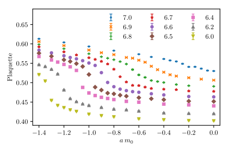
Figure 17: Value of the plaquette from a lattice parameter scan with dynamical fermions for lattice size of $4^{4}$, while varying the bare mass $am_{0}$ and the coupling $\beta$. The colours refer to the choices of $\beta$ indicated in the legend.

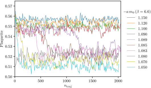
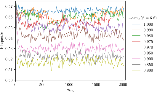
Figure 18: Trajectories of plaquette values for $\beta=6.6$ (top panel) and $\beta=6.8$ (bottom panel) on a lattice with size $8^{4}$, and for various values of the bare mass, as explained in the legend, from HMC calculations with dynamical quarks.

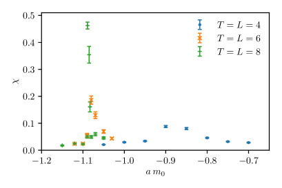
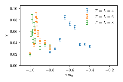
Figure 19: Plaquette susceptibilities $\chi$, measured in HMC calculations with dynamical quarks, for $\beta=6.6$ (top panel) and $\beta=6.8$ (bottom panel), as a function of the bare mass $am_{0}$, for three values of the lattice size (see legend).

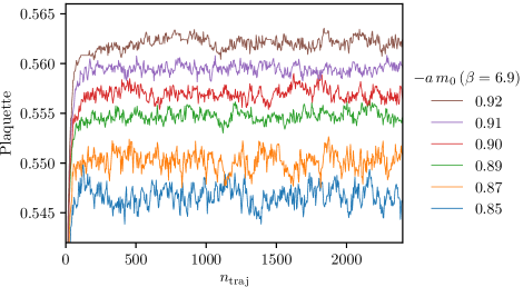
Figure 20: Trajectories of plaquette values for dynamical-fermion calculations at $\beta=6.9$. Different colours represent various fermion masses, as reported in the legend.

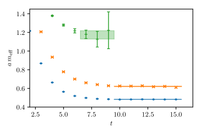
Figure 21: Effective mass plots for pseudo-scalar, vector, and axial-vector mesons at $\beta=6.9$ and $am_{0}=-0.91$. The shaded regions denote the fitting ranges and the statistical uncertainties of fit results.

The study of strongly-coupled gauge theories on discretised Euclidean space-time assumes the existence of a proper continuum limit as the lattice spacing $a$ decreases, so that the field-theory dynamics is recovered. In order to avoid uncontrollable systematic effects in the continuum extrapolation, one must explore the lattice parameter space to identify any singularities or bulk transitions before carrying out detailed numerical studies of physical observables. In particular, a bulk phase where lattice discretisation effects dominate the behaviour of the system is expected to be present at strong coupling, with the interesting physical region separated by this bulk region by a first-order phase transition, or a very sharp cross over.

The identification of the associated (pseudo-)critical coupling is also strongly desired for practical purposes, because with finite numerical resources one cannot reduce the lattice spacing to arbitrarily small values, while at the same time using large enough volumes. For the pure $Sp(4)$ lattice theory with the standard plaquette action the numerical study in Holland:2003kg shows the absence of bona-fide bulk phase transitions. To the best of our knowledge, no such a study for dynamical simulation with $N_{f}=2$ Wilson fermions exists in the literature.

A possible choice of order parameter associated with the lattice bulk transition is the expectation value of the plaquette. To have a rough mapping of the transition, we first scan the parameter space over the range of $\beta=[6.0,~{}7.0]$ using a $4^{4}$ lattice, and show the results in Fig. 17. For each lattice coupling, we calculate the average plaquette values and vary the bare mass in steps of $0.1$, over the range $0.0\leq-am_{0}\leq 1.4$. Near the region in which the change of the plaquette value is large as a function of $am_{0}$, we add twice more data points, to increase the resolution. The abrupt change of the plaquette expectation value, visible at smaller values of $\beta$, strongly suggests the presence of a bulk phase transition.

To find more concrete evidence of the bulk phase and determine the phase boundary, we increase the volume to $6^{4}$ and $8^{4}$ for two lattice couplings, $\beta=6.6$ and $6.8$. In Fig. 18 we plot the trajectories of the average plaquette measured on a $8^{4}$ lattice with various values of bare quark mass close to the transition. All configurations are generated from a cold start—the individual link is the unit matrix. The top panel for $\beta=6.6$ shows evidence of metastability at the critical mass which is expected for a first-order bulk phase transition. By comparison, in the bottom panel of Fig. 18, obtained for $\beta=6.8$, the plaquette values varies smoothly.

These results are further supported by measuring the plaquette susceptibility $\chi=(\langle\mathcal{P}^{2}\rangle-\langle\mathcal{P}\rangle^{2})\,V\,,$ and investigating the dependence of its maximum on the lattice four-volume $V$, as shown in Fig. 19. The peaks of $\chi$ from the largest two volumes roughly scale with $V$ for $\beta=6.6$, while they are almost constant for $\beta=6.8$, indicating cross-over behaviour.

From the combination of all these numerical results, we find that a conservative estimate of the minimum value of $\beta$ that ensures the existence of the continuum limit is $\beta\geq 6.8$. Based on this finding we perform fully dynamical simulations at $\beta=6.9$ as a very preliminary study of the meson spectrum. We generate six ensembles, $am_{0}=-0.85,\,-0.87$ on a $24\times 12^{3}$ and $am_{0}=-0.89,\,-0.9,\,-0.91,\,-0.92$ on a $32\times 16^{3}$ lattices, using the HMC algorithm.

In Fig. 20, we show the trajectories of the plaquette values. The asymptotic value of plaquette gradually increases as the bare fermion mass decreases. The typical thermalisation time appears to be $n_{\textrm{traj.}}\sim 300$, while the typical autocorrelation time ranges from $12$ to $32$, depending on the ensembles. The MD time steps for gauge and fermion actions are optimized such that the acceptance rate in the Metropolis test is in the range of $75-85\%$.

Fig. 21 shows the effective masses for pseudo-scalar, vector, and axial-vector mesons at $am_{0}=-0.91$, as an illustrative example. The pseudo-scalar and vector mesons clearly exhibit plateaux at large time, starting around $t=10$ and persisting over six time slices. These two mesons are much lighter than the UV cutoff and we find that $\frac{m_{\pi}}{m_{\rho}}\sim 0.8$. The best estimation of the axial-vector meson mass is carried out by fitting the effective mass for $t=[7\,,\,9]$, but the resulting mass is already at the scale of the UV cutoff $\sim 1/a$, as visible from Fig. 21. More interesting numerical studies including the EFT fits are beyond the aims of this paper: a dedicated investigation of systematic effects, such as those relevant to the scale-setting and the continuum extrapolation, has to be carried out, before we perform a detailed analysis of confronting the lattice data with the EFT.

8 Summary and Outlook

With this paper (see also Bennett:2017ttu ; Bennett:2017tum ; Bennett:2017kbp ), we have started a programme of systematic lattice studies of the dynamics of $Sp(2N)$ gauge theories with $N_{f}=2$ fundamental Dirac fermions and $N>1$. As explained in the Introduction, we envisage developing this programme along several distinct lines, of relevance in the contexts of composite-Higgs phenomenology, of composite fermions at strong coupling, and of thermodynamics at finite $T$ and $\mu$. We are also interested in the pure Yang-Mills theories ($N_{f}=0$), and in studying how the properties of these theories evolve as a function of $N$. We outlined here the whole programme, and took some important steps along these lines. We focused for the time being on $Sp(4)$, but constructed our numerical algorithms, data-analysis procedures and EFT treatment in such a way that they generalise straightforwardly to larger $N$. We conclude the paper by summarising our findings, and how they allow us to proceed to the next steps in the near future.

We performed preliminary, technical analyses of the $Sp(4)$ lattice gauge theory, and the results are shown in Sections 3 and 4. We used two different lattice algorithms; we successfully checked that the Hybrid Monte Carlo and Heat Bath both yield results that are compatible with each other as well as with those reported previously in the literature, having introduced an adequate re-symplectization procedure. We tested that the topological charge moves across sectors with dynamics suggesting good ergodicity properties and that the distributions of the ensembles for various choices of the lattice parameters do not show appreciable indications of severe autocorrelation. We also addressed the question of scale setting, by studying the gradient flow associated with the quantities $t_{0}$ and $w_{0}$ defined in the main body of the paper, and we found visible signals of quark-mass dependence. From the field-theory perspective, this may not come as a surprise, given that the RG flow is two-dimensional and non-trivial. Yet, it shows that in calculations with dynamical fermions one has to use extra caution in the process of extrapolating to the continuum limit. We expect that at least when the physical mass is small compared to the confinement scale, and for lattice calculations performed close enough to the continuum limit, the RG flow be driven mostly by the gauge coupling, with small dependence on the mass, as is the case of QCD Borsanyi:2012zs . We would like to collect evidence of this with values of lattice parameters beyond those employed in this paper (but see also Arthur:2016dir ; Ayyar:2017qdf ).

The main body of this paper mostly focused on the dynamics of the glue. In Sec. 5 we studied in detail the pure (Yang-Mills) $Sp(4)$ theory, showed that it confines in a way that is compatible with the effective string description, and performed the first detailed study of the spectrum of glueballs. We were able to perform the continuum-limit extrapolation of the latter, hence providing a set of determinations for the physical masses that is of quality comparable to the current state-of-the-art for other gauge theories. We could hence compare the spectrum of $Sp(4)$ to that of $SU(N)$ gauge theories, and in particular we found novel numerical support for two general expectations from the literature: the ratio $R$ between the masses of the lightest spin-2 and spin-0 glueballs is independent of the gauge group Athenodorou:2016ndx , and the ratio of the mass of the lightest spin-0 glueball to the string tension obeys Casimir scaling Hong:2017suj .

The long-term objective of this programme is the investigation of whether composite-Higgs models of new physics based upon the $SU(4)/Sp(4)$ coset are realistic and predictive. Having discussed the main features (and limitations) of the low-energy effective field theory description of pions, $\rho$, and $a_{1}$ mesons in Section 2, and postponing to the future the study of dynamical fermions, we performed a first, exploratory calculation of the masses and decay constants of the mesons in the quenched approximation, and reported the results in Sec. 6. The main purpose of this study is to show that the whole technology works effectively. We took particular care of precisely defining the operators of interest on the lattice, and of renormalizing the decay constants with one-loop matching coefficients. We performed the calculations by varying the value of the bare mass over a large range, while considering only two values of the lattice coupling $\beta$ and one choice of lattice volume.

We found several potentially interesting results for the mesons, although the preliminary nature of this quenched study implies that much caution has to be adopted. While we found that the spectra and decay constants of pions, $\rho$ and $a_{1}$ mesons can be fitted satisfactorily with the EFT description we provided, the spin-1 mesons are heavy with respect to the pion decay constant, and their coupling to the pions is large, hence bringing into serious question the reliability of the EFT description itself. We do not know whether this feature persists also with dynamical fermions, yet we expect an improvement with larger values of $N$, and hence find it encouraging that the fits within quenched $Sp(4)$ work well. We also found several other interesting features. For example, the special combination $f_{0}$ (defined in Sec. 2) of the decay constants of the mesons appears to be independent of the quark mass. It will be interesting to test such features beyond the quenched approximation, and possibly explaining them within field theory.

Finally, we uncovered evidence of a first-order (bulk) phase transition in the lattice theory with dynamical fermions, and presented in Sec. 7 the first results of the coarse scanning of the parameter space, hence identifying regions that are safely connected to the field theory in the continuum limit. We exemplified the calculations of the meson spectrum in the full dynamical theory for one choice of such parameters. A much more extensive study of the spectra would be needed to match to the expectations from field theory, particularly because of the subtleties involved in taking the continuum limit for generic, non-trivial values of the fermion mass. Having shown the feasibility of such a study with the instruments we put in place, we postpone to the future this extensive task.

The next steps of our programme will involve the following studies.

• We will compute the spectrum of glueballs in pure Yang-Mills for generic $Sp(2N)$. The HB algorithm has been already generalised to any $N$ and tested Bennett:2017kbp , and the process leading to the extraction of masses has been shown here to be robust. This will allow us to put the level of understanding of the spectra of $Sp(2N)$ Yang-Mills theories on the same level as the $SU(N)$ ones.

• The mass spectrum and decay constants of mesons will be studied with dynamical fermions, hence providing quantitative information of direct relevance to model-building and phenomenology in the context of composite-Higgs models of new physics.

• We want to extend the present study to be of relevance to the context of composite fermions, by generalising the underlying action to include fermionic matter in different representations. This is a novel direction for lattice studies, the very first such attempts having appeared only recently DeGrand:2015yna ; Ayyar:2017qdf . We envision to perform a preliminary study, possibly quenching part of the fermions, before attacking the non-trivial (and model-dependent) problem of analysing the properties of fermionic composite states.

Further in the future, we intend to extend the study of the mesons to other non-trivial dynamical properties of relevance to composite-Higgs models, such as the width of the excited mesons, and the value of the condensates. We are also interested in extending to $Sp(2N)$ the study of the high temperature behaviour of the theory, along the lines followed for $SU(2)\sim Sp(2)$ in Lee:2017uvl , and to introduce non-trivial chemical potential. Combinations of all these studies will provide a coherent framework within which to gain new insight of relevance for field theory, model building, and thermodynamics in extreme conditions.

MP would like to thank G. Ferretti for useful discussions. The work of EB and DV has been funded in part by the Supercomputing Wales project, which is part-funded by the European Regional Development Fund (ERDF) via Welsh Government. The work of DKH and JWL is supported in part by Korea Research Fellowship programme funded by the Ministry of Science, ICT and Future Planning through the National Research Foundation of Korea (2016H1D3A1909283) and under the framework of international cooperation programme (NRF-2016K2A9A1A01952069). The work of CJDL is supported by Taiwanese MoST grant 105-2628-M-009-003-MY4. The work of BL is supported in part by the Royal Society and the Wolfson Foundation. The work of BL, MP and DV has been supported in part by the STFC Consolidated Grants ST/L000369/1 and ST/P00055X/1.

Appendix A Some useful elements of group theory

We choose the generators of $SU(4)$ and of its $Sp(4)$ maximal subgroup as in Appendix B of Lee:2017uvl . We summarise some useful properties of the symplectic groups of interest, which we conventionally refer to as $Sp(2N)$, and the real algebra of which is denoted $C_{N}$ in Slansky:1981yr .

The group $Sp(2N)$ is defined as the set of $2N\times 2N$ unitary matrices $U$ with complex elements that satisfy the relation

$$U\Omega U^{T}=\Omega,$$ (106)

where $\Omega$ is the symplectic form, written—consistently with Eq. (6)—in $N\times N$ blocks as

$$\Omega=\begin{bmatrix}0&\mathbb{I}_{N}\\ -\mathbb{I}_{N}&0\\ \end{bmatrix}.$$ (107)

As suggested by Eq. (106), $U$ may be written in block form as

$$U=\begin{bmatrix}A&B\\ -B^{*}&A^{*}\\ \end{bmatrix}\,,$$ (108)

where $A$ and $B$ satisfy $A^{\dagger}A+B^{\dagger}B=\mathbb{I}$ and $A^{T}B=B^{T}A$. From these relations, we can deduce many properties of $Sp(2N)$ matrices. Having unit determinant, the matrices of $Sp(2N)$ can be shown to form a compact and simply connected subgroup of $SU(2N)$. Moreover, the structure in Eq. (108) implies that the centre of the group is isomorphic to $\mathbb{Z}_{2}$ for any $N$. Lastly, since $U^{*}=\Omega U\Omega^{T}$ and $\Omega\in Sp(2N)$, every representation of the group is equivalent to its complex conjugate. Thus $Sp(2N)$ has only pseudo-real representations, and charge conjugation is trivial.

In model-building as well as numerical applications, a prominent role is played by the subgroups of $Sp(2N)$, especially those isomorphic to some $SU(N)$. In particular, one notices that $Sp(2N)\subset SU(2N)$, and that $Sp(2(N-1))\subset Sp(2N)$. Starting with $Sp(2)\sim SU(2)$, this allows us to use the machinery already developed for the Monte Carlo simulation of $SU(2N)$ groups to the case of $Sp(2N)$. Particular attention has to be given to the choice of subgroups, as we further discuss in Appendix C in the HB context.

The subgroup structure of $Sp(2N)$ can be understood in terms of its algebra, to the study of which we now turn. Locally, one can represent a generic group element with the exponential map $U=\exp(\dot{\imath}H)$ and impose the constraints of $Sp(2N)$. This is equivalent to taking only the generators of $SU(2N)$ that satisfy Eq. (106), i.e. the hermitian traceless matrices with $H^{*}=\Omega H\Omega$, from which a block structure for $H$ follows,

$$H=\begin{bmatrix}A&B\\ B^{*}&-A^{*}\\ \end{bmatrix}.$$ (109)

The properties $A=A^{\dagger}$ and $B=B^{T}$ are a consequence of $H^{\dagger}=H$. These conditions leave a total of $2N(N+1)$ degrees of freedom for $H$, which is also the dimension of the $Sp(2N)$ group. The choice of generators that we use in this work is explicitly stated in Lee:2017uvl . The rank of the group is $N$, thus in $Sp(2N)$ we can find $N$ independent $SU(2)$ subgroups. Once the elements of the algebra have been chosen, the $SU(2)$ subgroups of $Sp(2N)$ follow from their matrix structure (see, once more, Appendix C).

Appendix B EFT and Technicolor

The 2-flavour $Sp(4)$ theory can be used as a technicolor (TC) model, provided the embedding of the SM symmetries is such that the condensate breaks them, and so can the EFT treatment we apply to the spin-1 states, provided we identify the natural $SU(2)_{L}^{t}\times SU(2)_{R}^{t}$ symmetries acting on the left-handed and right-handed components of $Q^{i\,a}$ as the SM global symmetry (following the conventions in Appendix B in Lee:2017uvl ). We added the superscript ^t to the weakly-coupled gauge groups to distinguish them from the embedding used in the body of this paper, in the context of composite-Higgs models The embedding is chosen so that $(SU(2)_{L}^{t}\times SU(2)_{R}^{t})\cap Sp(4)\,=\,SU(2)$, hence realising spontaneous symmetry breaking. One can then match this model to the familiar electroweak chiral Lagrangian and its extensions, based on the $(SU(2)\times SU(2))/SU(2)$ coset, which is practically advantageous as it allows to re-use well known results.

Gauge invariance of the electroweak theory in this case requires setting $M=0$, so that the pions are massless, and to gauge $SU(2)_{L}^{t}\times U(1)_{Y}^{t}$, where the latter factor is the subgroup of $SU(2)_{R}^{t}$ generated by the diagonal $t_{R}^{3}$. The gauge couplings are $\tilde{g}$ and $\tilde{g}^{\prime}$, respectively. By doing so, the exact symmetry is reduced from $SU(4)$ to $SU(2)^{t}_{L}\times U(1)^{t}_{Y}\times U(1)_{B}$, with the last abelian factor denoting baryon number. The condensate then breaks $SU(2)^{t}_{L}\times U(1)^{t}_{Y}\rightarrow U(1)_{\rm e.m.}$, and the $W$ and $Z$ bosons acquire a mass via the usual Higgs mechanism.

We discuss this TC model mostly for completeness, and for technical reasons related to the calculation of the 2-point functions. Among the phenomenological reasons why this is not a realistically viable TC model are the following.

• The spectrum contains two light (pseudo-)Goldstone bosons.

• Precision parameters such as $S$ might exceed experimental bounds.

• The spectrum does not contain a light scalar (Higgs) particle.

• There is no high scale to suppress higher-dimensional operators and FCNC transitions.

• There is no natural way to enhance the mass of the top quark.

We address here only the first two points, within the low-energy EFT, mostly for technical reasons that are of interest also in the composite-Higgs framework. We introduce the adjoint spurion $G$, formally transforming as

$$G \rightarrow U_{B}GU_{B}^{\dagger}\,,$$ (110)

and fix it to

$$G = \Lambda_{G}\,{\rm diag}\left\{\frac{}{}1\,,\,1\,,\,-1\,,\,-1\right\}\,,$$ (111)

We add to the Lagrangian density the additional (symmetry-breaking) term

$${\cal L}_{G} = \frac{\Lambda_{G}^{2}}{4}{\rm Tr\,}\left\{\frac{}{}G\left(S\Sigma S^{T}\right)G^{\ast}\left(S\Sigma S^{T}\right)^{\ast}\right\}\,,$$ (112)

in such a way as to induce the explicit breaking $SU(4)_{B}\rightarrow SU(2)_{L}^{t}\times SU(2)_{R}^{t}\times U(1)_{B}$. By expanding explicitly we find that

$${\cal L}_{G} = \Lambda_{G}^{4}\,-\,\Lambda_{G}^{4}\left(\frac{2S}{F}+\frac{2C}{f}\right)^{2}\left((\bar{\pi}^{4})^{\,2}+(\bar{\pi}^{5})^{\,2}\frac{}{}\right)\,+\,\cdots\,,$$ (113)

where $C$ and $S$ have been defined in Eqs. (31) and (32). We hence provided a mass for $\bar{\pi}^{4}$ and $\bar{\pi}^{5}$, while the massless $\bar{\pi}^{i}$ fields, with $i=1,2,3$, eventually become the longitudinal components of the $W$ and $Z$ bosons. In the limit $\Lambda_{G}\rightarrow+\infty$, $\bar{\pi}^{4}$ and $\bar{\pi}^{5}$ decouple completely, while the dynamics of the spin-1 states is unaffected, and the first of the phenomenological problems mentioned above is avoided.

We can now focus on the 2-point functions, by matching the theory defined by Eq. (2.1.2) onto the leading-order part of the effective Lagrangian for the transverse components of the SM gauge bosons $V^{i}_{\mu}=(L^{1}_{\mu},L^{2}_{\mu},L^{3}_{\mu},R^{3}_{\mu})$, which reads

$${\cal L}_{EFT} = \frac{1}{2}P^{\mu\nu}\Pi^{ij}(q^{2})V_{\mu}^{i}(q)V_{\nu}^{j}(-q)\,,$$ (114)

where $P^{\mu\nu}=-q^{\mu}q^{\nu}/q^{2}+\eta^{\mu\nu}$, $q^{\mu}$ is the four-momentum, and all the dynamics is contained in the non-trivial functions $\Pi^{ij}(q^{2})$.

The functions $\Pi^{ij}$ are defined by matching the (gaussian) path integrals (at the tree-level). In practice, one takes the second derivatives in respect to the $15+3+1=19$ gauge bosons $V_{\mu\,i}$ of the original theory $P^{\mu\nu}\Pi_{T}^{ij}\equiv P^{\mu\rho}\frac{\partial^{2}}{\partial V_{\rho i}\partial V_{\nu j}}{\cal L}=P^{\mu\nu}\left(q^{2}\delta^{ij}-({\cal M}^{2})^{\,ij}\right)$ (where ${\cal M}^{2}$ is the complete mass matrix of the vectors), then one inverts it and retains only the $4\times 4$ sub-matrix along the directions of $SU(2)_{L}^{t}\times U(1)_{R}^{t}$, and finally inverts it again to obtain $\Pi^{ij}=\left(\left(\Pi_{T}^{-1}\right)_{L,R}\right)^{-1}$.

Focusing on the $1$ and $2$ components of $\Pi^{ij}$, one can write $\Pi^{11}(q^{2})=\Pi^{22}(q^{2})=q^{2}-\frac{\tilde{g}^{2}}{4}\Sigma(q^{2})+{\cal O}(\tilde{g}^{2}/g_{\rho}^{2})$, and hence obtain the Left-Left current-current correlator in Eq. (22):

$$\Sigma(q^{2}) \equiv \lim_{\tilde{g}\rightarrow 0}\frac{4}{\tilde{g}^{2}}\left(\frac{}{}q^{2}-\Pi^{11}(q^{2})\right)\,.$$ (115)

By expanding $\Pi^{ij}(q^{2})$ in powers of $q^{2}$ one also obtains the precision electroweak parameters. They are defined by first normalising the fields $V_{\mu i}$ so that $\Pi^{\prime\,ii}(0)\equiv\left.\frac{\mbox{d}}{\mbox{d}q^{2}}\Pi^{ii}(q^{2})\right|_{q^{2}=0}=1$ for $i=1\,,\,\cdots\,,\,4$, and then defining Barbieri:2004qk

$$\hat{S} \equiv \frac{\tilde{g}}{\tilde{g}^{\prime}}\Pi^{\prime\,L^{3}R^{3}}(0)\,,\,\,\,\,\,\,\,\,\,\,\,\,\,\,\,\hat{T}\,\equiv\,\frac{1}{M_{W}^{2}}\left(\frac{}{}\Pi^{\prime\,L^{3}L^{3}}(0)-\Pi^{\prime\,L^{2}L^{2}}(0)\right)\,.$$ (116)

In the current case, one finds that $\hat{T}=0$, because of the custodial $SU(2)$, while the experimental bounds obtained from precision parameters are $\hat{S}<0.003$ (at $3\sigma$ c.l.) Barbieri:2004qk .

A subtlety should be noted here: the structure of the effective Lagrangian describing all the vectors in the case of relevance for TC should include additional terms in respect to Eq. (2.1.2), as in this case the condensate breaks the $SU(2)_{L}^{t}$ symmetry. For example, this yields kinetic mixing between the $W$ and $B$ gauge bosons, which contributes directly to the $\hat{S}$ parameter, and can be thought of as the contribution to $\hat{S}$ coming from heavier composite states that have been integrated out. We do not include such terms, because they go beyond the purposes of this paper.

If one applies the formalism described here to the Lagrangian density in Eq. (2.1.2), what results is not the $S$ parameter, but rather the contribution to $S$ coming from $\rho$ and $a_{1}$ mesons only, which we called $S_{0}$. We notice that the following sum rule (occasionally referred to as zeroth order in the literature) is verified exactly within the framework defined by Eq. (2.1.2):

$$\frac{S_{0}}{4\pi} = \frac{f_{\rho}^{2}}{M_{\rho}^{2}}-\frac{f_{a_{1}}^{2}}{M_{a_{1}}^{2}}\,.$$ (117)

We can express this result explicitly in terms of the coefficients in the EFT Lagrangian density:

$$\frac{S_{0}}{4\pi} = \frac{2}{{g_{\rho}^{2}}}\left(1+\kappa+m\,y_{3}-\frac{(1-\kappa-m\,y_{4})(-b{f^{2}}+{F^{2}}+2{m}({v_{2}}-{v_{1}}))^{2}}{((2b+4){f^{2}}+2mv_{2}-bf^{2}+{F^{2}}+2{m}(v_{2}-{v_{1}}))^{2}}\right)\,.$$ (118)

We stress once more that this result holds only within the EFT in Eq. (2.1.2), but not in the fundamental theory, for which one would have to replace the right-hand side of Eq. (117) with a summation over all possible spin-1 states, not just the ground state. To include such contributions in the EFT would require introducing explicit symmetry-breaking terms in $\cal L$ of the form of kinetic mixing terms that are forbidden within the composite-Higgs scenario, and are hence omitted here.

We conclude with an exercise. By making use of the quenched calculations reported in subsection 6.2, and of the fits of the low-energy couplings in Eq. (2.1.2), we find that $S_{0}/4\pi\sim 0.049$ (for $\beta=7.62$), and $S_{0}/4\pi\sim 0.041$ (for $\beta=8.0$). The large values of $S_{0}$, in respect to QCD (for which the same treatment would yield $S_{0}/4\pi\sim 0.025$, obtained by just replacing the masses and decay constants from experiments Patrignani:2016xqp ), might be due, at least in part, to the dimension of the gauge group $Sp(4)$ being larger than that of QCD. Yet these numerical results show a significant decrease in approaching the continuum limit, and are affected by quenching, hence they must be taken as just for illustration purposes.

Appendix C Projecting on $Sp(4)$

The update of local gauge links must be supplemented by a projection onto the $Sp(4)$ group manifold, to remove machine-precision effects that would bring the algorithm outside of the group manifold. In this Appendix we explain how we implement this re-symplectisation procedure.

The generic $Sp(2N)$ elements can be represented by $2N\times 2N$ complex matrices composed of quaternions,

$$Q(x,\mu)=Q_{0}(x,\mu)\otimes\mathbb{I}_{2}+Q_{1}(x,\mu)\otimes e_{1}+Q_{2}(x,\mu)\otimes e_{2}+Q_{3}(x,\mu)\otimes e_{3},$$ (119)

where the quaternion units are

$$\mathbb{I}_{2}=\left(\begin{array}[]{cc}1&0\\ 0&1\end{array}\right),~{}e_{1}=\left(\begin{array}[]{cc}i&0\\ 0&-i\end{array}\right),~{}e_{2}=\left(\begin{array}[]{cc}0&1\\ -1&0\end{array}\right),~{}e_{3}=\left(\begin{array}[]{cc}0&i\\ i&0\end{array}\right).$$ (120)

$Q_{i}(x,\mu)$ are $N\times N$ real matrices. Given the updated link variables $U(x,\mu)$ in the HMC algorithm, we project it onto the quaternion basis and normalise it, hence obtaining a symplectic $U(x,\mu)$ ahead of the Metropolis test.

To gauge the potential size of the violation of symplectic conditions and the importance of the $Sp(4)$ projection, we plot in Fig. 22 the trajectories of the plaquette values with (top) and without (bottom) re-symplectisation. The result shows that the re-symplectisation is successfully working and the plaquette values are stable.

In the HB calculations, we use instead a variant of the (modified) Gram-Schmidt algorithm. A re-symplectisation algorithm that inherits the numerical stability of the Gram-Schmidt process and that can be applied to any $N$ is obtained by noting that, owing to the general form of $Sp(2N)$ matrices, once the first $N$ columns of the matrix are known, the remaining ones can be computed from

$$col_{j+N}=-\Omega~{}col_{j}^{*}.$$ (121)

After normalising the first column, one can obtain the $(N+1)$-th. The second column is then obtained by orthonormalisation with respect to the first and the $(N+1)$-th. Repeating the process for every column, one obtains an $Sp(2N)$ matrix.

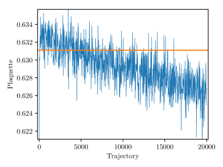
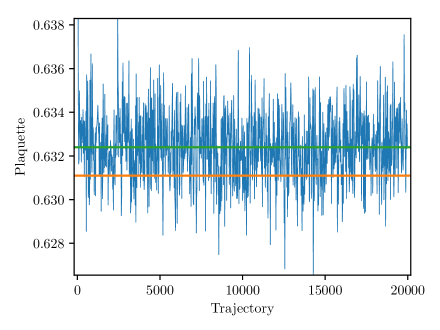
Figure 22: Trajectories of plaquette values without (top panel) and with (bottom panel) resymplectization, as described in Appendix C. The orange band denotes the quenched result in Holland:2003kg , while the green band denotes the fit result. The lattice parameters are $\beta=8.0$, $m_{0}=1.0$, and $N_{t}\times N_{s}^{3}=8\times 8^{3}$.

References

- (1) K. Holland, M. Pepe and U. J. Wiese, Nucl. Phys. B 694, 35 (2004) doi:10.1016/j.nuclphysb.2004.06.026 [hep-lat/0312022].
- (2) G. Aad et al. [ATLAS Collaboration], Phys. Lett. B 716, 1 (2012) doi:10.1016/j.physletb.2012.08.020 [arXiv:1207.7214 [hep-ex]].
- (3) S. Chatrchyan et al. [CMS Collaboration], Phys. Lett. B 716, 30 (2012) doi:10.1016/j.physletb.2012.08.021 [arXiv:1207.7235 [hep-ex]].
- (4) D. B. Kaplan and H. Georgi, Phys. Lett. 136B, 183 (1984). doi:10.1016/0370-2693(84)91177-8
- (5) H. Georgi and D. B. Kaplan, Phys. Lett. 145B, 216 (1984). doi:10.1016/0370-2693(84)90341-1
- (6) M. J. Dugan, H. Georgi and D. B. Kaplan, Nucl. Phys. B 254, 299 (1985). doi:10.1016/0550-3213(85)90221-4
- (7) K. Agashe, R. Contino and A. Pomarol, Nucl. Phys. B 719, 165 (2005) doi:10.1016/j.nuclphysb.2005.04.035 [hep-ph/0412089].
- (8) E. Katz, A. E. Nelson and D. G. E. Walker, JHEP 0508, 074 (2005) doi:10.1088/1126-6708/2005/08/074 [hep-ph/0504252].
- (9) R. Contino, L. Da Rold and A. Pomarol, Phys. Rev. D 75, 055014 (2007) doi:10.1103/PhysRevD.75.055014 [hep-ph/0612048].
- (10) R. Barbieri, B. Bellazzini, V. S. Rychkov and A. Varagnolo, Phys. Rev. D 76, 115008 (2007) doi:10.1103/PhysRevD.76.115008 [arXiv:0706.0432 [hep-ph]].
- (11) P. Lodone, JHEP 0812, 029 (2008) doi:10.1088/1126-6708/2008/12/029 [arXiv:0806.1472 [hep-ph]].
- (12) G. Ferretti and D. Karateev, JHEP 1403, 077 (2014) doi:10.1007/JHEP03(2014)077 [arXiv:1312.5330 [hep-ph]].
- (13) G. Cacciapaglia and F. Sannino, JHEP 1404, 111 (2014) doi:10.1007/JHEP04(2014)111 [arXiv:1402.0233 [hep-ph]].
- (14) A. Arbey, G. Cacciapaglia, H. Cai, A. Deandrea, S. Le Corre and F. Sannino, Phys. Rev. D 95, no. 1, 015028 (2017) doi:10.1103/PhysRevD.95.015028 [arXiv:1502.04718 [hep-ph]].
- (15) L. Vecchi, JHEP 1702, 094 (2017) doi:10.1007/JHEP02(2017)094 [arXiv:1506.00623 [hep-ph]].
- (16) G. Panico and A. Wulzer, Lect. Notes Phys. 913, pp.1 (2016) doi:10.1007/978-3-319-22617-0 [arXiv:1506.01961 [hep-ph]].
- (17) G. Ferretti, JHEP 1606, 107 (2016) doi:10.1007/JHEP06(2016)107 [arXiv:1604.06467 [hep-ph]].
- (18) A. Agugliaro, O. Antipin, D. Becciolini, S. De Curtis and M. Redi, Phys. Rev. D 95, no. 3, 035019 (2017) doi:10.1103/PhysRevD.95.035019 [arXiv:1609.07122 [hep-ph]].
- (19) T. Alanne, D. Buarque Franzosi and M. T. Frandsen, Phys. Rev. D 96, no. 9, 095012 (2017) doi:10.1103/PhysRevD.96.095012 [arXiv:1709.10473 [hep-ph]].
- (20) F. Feruglio, B. Gavela, K. Kanshin, P. A. N. Machado, S. Rigolin and S. Saa, JHEP 1606, 038 (2016) doi:10.1007/JHEP06(2016)038 [arXiv:1603.05668 [hep-ph]].
- (21) S. Fichet, G. von Gersdorff, E. Pont n and R. Rosenfeld, JHEP 1609, 158 (2016) doi:10.1007/JHEP09(2016)158 [arXiv:1607.03125 [hep-ph]].
- (22) J. Galloway, A. L. Kagan and A. Martin, Phys. Rev. D 95, no. 3, 035038 (2017) doi:10.1103/PhysRevD.95.035038 [arXiv:1609.05883 [hep-ph]].
- (23) T. Alanne, D. Buarque Franzosi, M. T. Frandsen, M. L. A. Kristensen, A. Meroni and M. Rosenlyst, arXiv:1711.10410 [hep-ph].
- (24) C. Csaki, T. Ma and J. Shu, Phys. Rev. Lett. 119, no. 13, 131803 (2017) doi:10.1103/PhysRevLett.119.131803 [arXiv:1702.00405 [hep-ph]].
- (25) M. Chala, G. Durieux, C. Grojean, L. de Lima and O. Matsedonskyi, JHEP 1706, 088 (2017) doi:10.1007/JHEP06(2017)088 [arXiv:1703.10624 [hep-ph]].
- (26) B. Gripaios, A. Pomarol, F. Riva and J. Serra, JHEP 0904, 070 (2009) doi:10.1088/1126-6708/2009/04/070 [arXiv:0902.1483 [hep-ph]].
- (27) J. Barnard, T. Gherghetta and T. S. Ray, JHEP 1402, 002 (2014) doi:10.1007/JHEP02(2014)002 [arXiv:1311.6562 [hep-ph]].
- (28) R. Lewis, C. Pica and F. Sannino, Phys. Rev. D 85, 014504 (2012) doi:10.1103/PhysRevD.85.014504 [arXiv:1109.3513 [hep-ph]].
- (29) A. Hietanen, R. Lewis, C. Pica and F. Sannino, JHEP 1407, 116 (2014) doi:10.1007/JHEP07(2014)116 [arXiv:1404.2794 [hep-lat]].
- (30) R. Arthur, V. Drach, M. Hansen, A. Hietanen, C. Pica and F. Sannino, Phys. Rev. D 94, no. 9, 094507 (2016) doi:10.1103/PhysRevD.94.094507 [arXiv:1602.06559 [hep-lat]].
- (31) R. Arthur, V. Drach, A. Hietanen, C. Pica and F. Sannino, arXiv:1607.06654 [hep-lat].
- (32) C. Pica, V. Drach, M. Hansen and F. Sannino, EPJ Web Conf. 137, 10005 (2017) doi:10.1051/epjconf/201713710005 [arXiv:1612.09336 [hep-lat]].
- (33) W. Detmold, M. McCullough and A. Pochinsky, Phys. Rev. D 90, no. 11, 114506 (2014) doi:10.1103/PhysRevD.90.114506 [arXiv:1406.4116 [hep-lat]].
- (34) J. W. Lee, B. Lucini and M. Piai, JHEP 1704, 036 (2017) doi:10.1007/JHEP04(2017)036 [arXiv:1701.03228 [hep-lat]].
- (35) G. Cacciapaglia, H. Cai, A. Deandrea, T. Flacke, S. J. Lee and A. Parolini, JHEP 1511, 201 (2015) doi:10.1007/JHEP11(2015)201 [arXiv:1507.02283 [hep-ph]].
- (36) D. K. Hong, arXiv:1703.05081 [hep-ph].
- (37) M. Golterman and Y. Shamir, arXiv:1707.06033 [hep-ph].
- (38) N. Bizot, M. Frigerio, M. Knecht and J. L. Kneur, Phys. Rev. D 95, no. 7, 075006 (2017) doi:10.1103/PhysRevD.95.075006 [arXiv:1610.09293 [hep-ph]].
- (39) B. Lucini and M. Panero, Phys. Rept. 526, 93 (2013) doi:10.1016/j.physrep.2013.01.001 [arXiv:1210.4997 [hep-th]].
- (40) B. Lucini, M. Teper and U. Wenger, JHEP 0406, 012 (2004) doi:10.1088/1126-6708/2004/06/012 [hep-lat/0404008].
- (41) A. Athenodorou, R. Lau and M. Teper, Phys. Lett. B 749, 448 (2015) doi:10.1016/j.physletb.2015.08.023 [arXiv:1504.08126 [hep-lat]].
- (42) R. Lau and M. Teper, JHEP 1710, 022 (2017) doi:10.1007/JHEP10(2017)022 [arXiv:1701.06941 [hep-lat]].
- (43) A. Athenodorou, E. Bennett, G. Bergner, D. Elander, C.-J. D. Lin, B. Lucini and M. Piai, JHEP 1606, 114 (2016) doi:10.1007/JHEP06(2016)114 [arXiv:1605.04258 [hep-th]].
- (44) D. K. Hong, J. W. Lee, B. Lucini, M. Piai and D. Vadacchino, Phys. Lett. B 775, 89 (2017) doi:10.1016/j.physletb.2017.10.050 [arXiv:1705.00286 [hep-th]].
- (45) M. Bando, T. Kugo, S. Uehara, K. Yamawaki and T. Yanagida, Phys. Rev. Lett. 54, 1215 (1985). doi:10.1103/PhysRevLett.54.1215
- (46) R. Casalbuoni, S. De Curtis, D. Dominici and R. Gatto, Phys. Lett. 155B, 95 (1985). doi:10.1016/0370-2693(85)91038-X
- (47) M. Bando, T. Kugo and K. Yamawaki, Phys. Rept. 164, 217 (1988). doi:10.1016/0370-1573(88)90019-1
- (48) R. Casalbuoni, S. De Curtis, D. Dominici, F. Feruglio and R. Gatto, Int. J. Mod. Phys. A 4, 1065 (1989). doi:10.1142/S0217751X89000492
- (49) M. Harada and K. Yamawaki, Phys. Rept. 381, 1 (2003) doi:10.1016/S0370-1573(03)00139-X [hep-ph/0302103].
- (50) H. Georgi, Nucl. Phys. B 331, 311 (1990). doi:10.1016/0550-3213(90)90210-5
- (51) T. Appelquist, P. S. Rodrigues da Silva and F. Sannino, Phys. Rev. D 60, 116007 (1999) doi:10.1103/PhysRevD.60.116007 [hep-ph/9906555].
- (52) M. Piai, A. Pierce and J. G. Wacker, hep-ph/0405242.
- (53) D. Buarque Franzosi, G. Cacciapaglia, H. Cai, A. Deandrea and M. Frandsen, JHEP 1611, 076 (2016) doi:10.1007/JHEP11(2016)076 [arXiv:1605.01363 [hep-ph]].
- (54) T. DeGrand, M. Golterman, E. T. Neil and Y. Shamir, Phys. Rev. D 94, no. 2, 025020 (2016) doi:10.1103/PhysRevD.94.025020 [arXiv:1605.07738 [hep-ph]].
- (55) M. Luscher, Nucl. Phys. B 364, 237 (1991). doi:10.1016/0550-3213(91)90584-K
- (56) X. Feng, K. Jansen and D. B. Renner, Phys. Rev. D 83, 094505 (2011) doi:10.1103/PhysRevD.83.094505 [arXiv:1011.5288 [hep-lat]].
- (57) L. Del Debbio, A. Patella and C. Pica, Phys. Rev. D 81, 094503 (2010) doi:10.1103/PhysRevD.81.094503 [arXiv:0805.2058 [hep-lat]].
- (58) N. Cabibbo and E. Marinari, Phys. Lett. 119B, 387 (1982). doi:10.1016/0370-2693(82)90696-7
- (59) T. Takaishi, Comput. Phys. Commun. 133, 6 (2000) doi:10.1016/S0010-4655(00)00161-2 [hep-lat/9909134].
- (60) M. Creutz, Phys. Rev. D 38, 1228 (1988). doi:10.1103/PhysRevD.38.1228
- (61) M. Luscher, Commun. Math. Phys. 293, 899 (2010) doi:10.1007/s00220-009-0953-7 [arXiv:0907.5491 [hep-lat]].
- (62) M. L scher, JHEP 1008, 071 (2010) Erratum: [JHEP 1403, 092 (2014)] doi:10.1007/JHEP08(2010)071, 10.1007/JHEP03(2014)092 [arXiv:1006.4518 [hep-lat]].
- (63) M. Luscher and P. Weisz, JHEP 1102, 051 (2011) doi:10.1007/JHEP02(2011)051 [arXiv:1101.0963 [hep-th]].
- (64) K. Fujikawa, JHEP 1603, 021 (2016) doi:10.1007/JHEP03(2016)021 [arXiv:1601.01578 [hep-lat]].
- (65) S. Borsanyi et al., JHEP 1209, 010 (2012) doi:10.1007/JHEP09(2012)010 [arXiv:1203.4469 [hep-lat]].
- (66) Z. Fodor, K. Holland, J. Kuti, S. Mondal, D. Nogradi and C. H. Wong, JHEP 1409, 018 (2014) doi:10.1007/JHEP09(2014)018 [arXiv:1406.0827 [hep-lat]].
- (67) A. Ramos and S. Sint, Eur. Phys. J. C 76, no. 1, 15 (2016) doi:10.1140/epjc/s10052-015-3831-9 [arXiv:1508.05552 [hep-lat]].
- (68) C.-J. D. Lin, K. Ogawa and A. Ramos, JHEP 1512, 103 (2015) doi:10.1007/JHEP12(2015)103 [arXiv:1510.05755 [hep-lat]].
- (69) M. Luscher and S. Schaefer, JHEP 1107, 036 (2011) doi:10.1007/JHEP07(2011)036 [arXiv:1105.4749 [hep-lat]].
- (70) D. Galletly, M. Gurtler, R. Horsley, H. Perlt, P. E. L. Rakow, G. Schierholz, A. Schiller and T. Streuer, Phys. Rev. D 75, 073015 (2007) doi:10.1103/PhysRevD.75.073015 [hep-lat/0607024].
- (71) M. Luscher, K. Symanzik and P. Weisz, Nucl. Phys. B 173, 365 (1980). doi:10.1016/0550-3213(80)90009-7
- (72) J. Polchinski and A. Strominger, Phys. Rev. Lett. 67, 1681 (1991). doi:10.1103/PhysRevLett.67.1681
- (73) M. Luscher, Nucl. Phys. B 180, 317 (1981). doi:10.1016/0550-3213(81)90423-5
- (74) B. Lucini and M. Teper, Phys. Rev. D 64, 105019 (2001) doi:10.1103/PhysRevD.64.105019 [hep-lat/0107007].
- (75) S. Necco and R. Sommer, Nucl. Phys. B 622, 328 (2002) doi:10.1016/S0550-3213(01)00582-X [hep-lat/0108008].
- (76) A. Athenodorou, B. Bringoltz and M. Teper, JHEP 1102, 030 (2011) doi:10.1007/JHEP02(2011)030 [arXiv:1007.4720 [hep-lat]].
- (77) M. Luscher and P. Weisz, JHEP 0407, 014 (2004) doi:10.1088/1126-6708/2004/07/014 [hep-th/0406205].
- (78) O. Aharony and E. Karzbrun, JHEP 0906, 012 (2009) doi:10.1088/1126-6708/2009/06/012 [arXiv:0903.1927 [hep-th]].
- (79) J. M. Drummond, hep-th/0411017.
- (80) N. D. Hari Dass and P. Matlock, hep-th/0606265.
- (81) J. M. Drummond, hep-th/0608109.
- (82) N. D. H. Dass and P. Matlock, hep-th/0611215.
- (83) O. Aharony and Z. Komargodski, JHEP 1305, 118 (2013) doi:10.1007/JHEP05(2013)118 [arXiv:1302.6257 [hep-th]].
- (84) S. Dubovsky and V. Gorbenko, JHEP 1602, 022 (2016) doi:10.1007/JHEP02(2016)022 [arXiv:1511.01908 [hep-th]].
- (85) B. Berg and A. Billoire, Nucl. Phys. B 221, 109 (1983). doi:10.1016/0550-3213(83)90620-X
- (86) C. J. Morningstar and M. J. Peardon, Phys. Rev. D 56, 4043 (1997) doi:10.1103/PhysRevD.56.4043 [hep-lat/9704011].
- (87) C. J. Morningstar and M. J. Peardon, Phys. Rev. D 60, 034509 (1999) doi:10.1103/PhysRevD.60.034509 [hep-lat/9901004].
- (88) J. Hoek, M. Teper and J. Waterhouse, Nucl. Phys. B 288, 589 (1987). doi:10.1016/0550-3213(87)90230-6
- (89) B. Lucini, A. Rago and E. Rinaldi, JHEP 1008, 119 (2010) doi:10.1007/JHEP08(2010)119 [arXiv:1007.3879 [hep-lat]].
- (90) B. Lucini and M. Teper, JHEP 0106, 050 (2001) doi:10.1088/1126-6708/2001/06/050 [hep-lat/0103027].
- (91) C. W. Bernard and M. F. L. Golterman, Phys. Rev. D 46, 853 (1992) doi:10.1103/PhysRevD.46.853 [hep-lat/9204007].
- (92) S. R. Sharpe, Phys. Rev. D 46, 3146 (1992) doi:10.1103/PhysRevD.46.3146 [hep-lat/9205020].
- (93) S. R. Sharpe and N. Shoresh, Phys. Rev. D 62, 094503 (2000) doi:10.1103/PhysRevD.62.094503 [hep-lat/0006017].
- (94) S. R. Sharpe and N. Shoresh, Phys. Rev. D 64, 114510 (2001) doi:10.1103/PhysRevD.64.114510 [hep-lat/0108003].
- (95) C. W. Bernard and M. F. L. Golterman, Phys. Rev. D 49, 486 (1994) doi:10.1103/PhysRevD.49.486 [hep-lat/9306005].
- (96) G. Martinelli and Y. C. Zhang, Phys. Lett. 123B, 433 (1983). doi:10.1016/0370-2693(83)90987-5
- (97) G. P. Lepage and P. B. Mackenzie, Phys. Rev. D 48, 2250 (1993) doi:10.1103/PhysRevD.48.2250 [hep-lat/9209022].
- (98) P. A. Boyle, A. Juttner, C. Kelly and R. D. Kenway, JHEP 0808, 086 (2008) doi:10.1088/1126-6708/2008/08/086 [arXiv:0804.1501 [hep-lat]].
- (99) E. Bennett, D. K. Hong, J. W. Lee, C.-J. D. Lin, B. Lucini, M. Piai and D. Vadacchino, arXiv:1710.06941 [hep-lat].
- (100) E. Bennett, D. K. Hong, J. W. Lee, C.-J. D. Lin, B. Lucini, M. Piai and D. Vadacchino, arXiv:1710.06715 [hep-lat].
- (101) E. Bennett, D. K. Hong, J. W. Lee, C.-J. D. Lin, B. Lucini, M. Piai and D. Vadacchino, arXiv:1710.07043 [hep-lat].
- (102) V. Ayyar, T. DeGrand, M. Golterman, D. C. Hackett, W. I. Jay, E. T. Neil, Y. Shamir and B. Svetitsky, arXiv:1710.00806 [hep-lat].
- (103) T. DeGrand and Y. Shamir, Phys. Rev. D 92, no. 7, 075039 (2015) doi:10.1103/PhysRevD.92.075039 [arXiv:1508.02581 [hep-ph]].
- (104) R. Slansky, Phys. Rept. 79, 1 (1981). doi:10.1016/0370-1573(81)90092-2
- (105) R. Barbieri, A. Pomarol, R. Rattazzi and A. Strumia, Nucl. Phys. B 703, 127 (2004) doi:10.1016/j.nuclphysb.2004.10.014 [hep-ph/0405040].
- (106) M. E. Peskin and T. Takeuchi, Phys. Rev. D 46, 381 (1992). doi:10.1103/PhysRevD.46.381
- (107) T. Appelquist et al. [LSD Collaboration], Phys. Rev. Lett. 106, 231601 (2011) doi:10.1103/PhysRevLett.106.231601 [arXiv:1009.5967 [hep-ph]].
- (108) P. A. Boyle et al. [RBC and UKQCD Collaborations], Phys. Rev. D 81, 014504 (2010) doi:10.1103/PhysRevD.81.014504 [arXiv:0909.4931 [hep-lat]].
- (109) C. Patrignani et al. [Particle Data Group], Chin. Phys. C 40, no. 10, 100001 (2016). doi:10.1088/1674-1137/40/10/100001