Divergences of the irreducible vertex functions in correlated metallic systems:
Insights from the Anderson impurity model

Abstract

In this work, we analyze in detail the occurrence of divergences in the irreducible vertex functions for one of the fundamental models of many-body physics: the Anderson impurity model (AIM). These divergences, a surprising hallmark of the breakdown of many-electron perturbation theory – have been recently observed in several contexts, including the dynamical mean-field solution of the Hubbard model. The numerical calculations for the AIM presented in this work, as well as their comparison with the corresponding results for the Hubbard model, allow us to clarify several open questions about the properties of vertex divergences in a particularly interesting context, the correlated metallic regime at low-temperatures. Specifically, our analysis (i) rules out explicitly the transition to a Mott insulating phase, but not the more general suppression of charge fluctuations (proposed in [O. Gunnarsson et al., Phys. Rev. B 93, 245102 (2016)]), as a necessary condition for the occurrence of vertex divergences, (ii) clarifies their relation with the underlying Kondo physics, and, eventually, (iii) individuates which divergences might also appear on the real frequency axis in the limit of zero temperature, through the discovered scaling properties of the singular eigenvectors.

I Introduction

The foundation of the Feynman diagrammatic technique relies on the many-body perturbation expansion. Nonetheless, its high flexibility and the transparency of the physical interpretation have often motivated the application of diagrammatic schemes also well beyond the perturbative regime. This is particularly true for the many-electron problem in condensed matter theory. In fact, for the latter, the identification of a small parameter controlling the perturbation expansion can become a very hard task, especially if the Coulomb interaction is not sufficiently screened, a common situation in transition metal oxides and heavy fermion compounds.

In general, exploiting diagrammatic techniques beyond the regime of validity of the underlying perturbation expansion is a viable option, and – in some cases – also a rewarding one, as witnessed, e.g., by the success of the Dynamical Mean-Field Theory (DMFT)DMFTREV and its extensionsDCAREV ; Rohringer_REV . However, in doing so, one must expect to face particular problems, which might limit the applicability of well known diagrammatic relations and challenge the corresponding algorithmic implementations in the strong-coupling regime. Not surprisingly, considering the fast developments of the diagrammatic extensionsDGA ; DF ; DB ; 1PI ; DMF2RG ; TRILEX ; DMFT_FLEX ; QUADRILEX ; Rohringer_REV of DMFT, some of these issues have been recently put in the focus of the forefront literature on quantum many-body theory.

In particular, two main kind of problems have been brought to lightSchaefer2013 ; Kozik2015 and analyzed. The first one is the occurrence of divergences of the two-particle irreducible (2PI) vertex functions in several many-electron models. In fact, their occurrence has been reported, even for moderate values of the electronic interaction, in DMFT studies of the disordered binary mixture (BM)Schaefer2016 , the Falicov Kimball (FK)Schaefer2013 ; Schaefer2016 ; Janis2014 ; Ribic2016 and the Hubbard modelSchaefer2013 ; Schaefer2016 ; Rohringer_Diss ; Vucevia2018 . Analytical calculationsSchaefer2013 ; Schaefer2016 ; Rohringer_Diss ; Stan2015 for the atomic limit (AL) of the Hubbard modelHubbard or the one point modelLani2012 ; Berger2014 have provided further evidence of the robustness and the generality of the occurrence of these divergences of the 2PI vertex. Finally, calculations with the dynamical cluster approximation (DCA) have also demonstratedGunnarsson2016 ; Vucevia2018 that the observed divergences are not an artifact of the purely local treatment of DMFT. The irreducible vertex divergences appear as a consequence of the non-invertibility of the Bethe-Salpeter equation in the fermionic Matsubara frequency space (see Sec. II), associated with a simultaneousSchaefer2016 non-invertibility of the parquet equations. In specific cases (FKJanis2014 ; Ribic2016 ; Schaefer2016 , BMSchaefer2016 ), their presence has been also reported on the real frequency axis.

The second problem reported Kozik2015 ; Schaefer2016 ; Stan2015 ; Rossi2015 ; Keiter ; Gunnarsson2017 ; Vucevia2018 is an intrinsic multivaluedness of the Luttinger Ward functional (LWF). This unexpected characteristic of the LWF has been demonstratedKozik2015 by considering the self-consistent (bold) perturbation expansion for the self-energy $\Sigma[G]$ in the AL of the Hubbard model, for which the exact Green’s function is known analytically. The corresponding resummation is found always to converge but, for interaction values $U$ larger than a specific $\widetilde{U}$, it converges to unphysical results, indicating the existence of at least two branches of the LWF for the self-energy.

Eventually, recent studiesGunnarsson2017 have rigorously demonstrated that these two aspects are exactly related, providing an analytic proof that any crossing of different branches in the LWF functional is associated to a divergence of the 2PI vertex, occurring for the same parameters (see Sec. A in the Supplemental Material of Ref. [Gunnarsson2017, ]).

From a purely theoretical viewpoint, these problems can be regarded as complementary manifestations of the breakdown of the perturbation expansion. At the same time, from a more practical perspective, their potential impact on several cutting edge algorithmic developments can also be significant. In particular, we recall that the 2PI vertex functions constitute the fundamental building block of all diagrammatic theories based on the Bethe-Salpeter or parquet equationsBickers ; Yang2009 ; Tam2013 ; Li2017 , such as, e.g., the dynamical vertex approximation (D$\Gamma$A)DGA ; Toschi2011 ; Galler2017 , the multiscaleSlezak2009 , and the quadruply-irreducible local expansion (QUADRILEX)QUADRILEX approach, or the parquet decomposition of the self-energyGunnarsson2016 . Similarly, the presence of multiple branches in the LWF might pose difficulties to bold diagrammatic Monte Carlo schemesKozik2015 ; Tarantino2017 ; Vucevia2018 . The discussion on how (and to what extent) it is possible to circumvent these difficulties within the different algorithms is a subject of current scientific debatenote_wayouts .

One should mention, moreover, that the interpretation of the physics underlying this twofold manifestation of the breakdown of the perturbation expansion is still debated. Certainly, these crossings and divergences are not associated with any thermodynamic phase transition, due to the mutual compensation of (divergent) irreducible and fully irreducible diagrams in the parquet equations, which ensures, that the full vertex stays finite (see Sec. II.2). It has been proposedSchaefer2013 ; Janis2014 ; Schaefer2016 , however, that they might be interpreted, for example, as precursors of the Mott metal-insulator transitionMH (MIT), as features of the separation of spectral weight (such as the Hubbard subbands), as an implication of the emergence of kinks in the spectral functionByzuk2007 ; Held2013 and specific heatToschi2009 ; Toschi2010 , and even in terms of qualitative changes in the non-equilibrium asymptotic behaviorsSchaefer2013 . Subsequently, it has been arguedGunnarsson2016 ; Gunnarsson2017 , that their occurrence in the Hubbard model is associated with the progressive suppression of the charge susceptibility for increasing values of the electrostatic repulsion $U$.

The aim of this paper is to improve our current understanding of the properties of the 2PI-vertex divergences, especially in the arguably most interesting parameter regime of low-temperatures and moderate interaction values, where they appear to coexist with a metallic, Fermi-Liquid ground state.

This will provide, in turn, hitherto missing pieces of information about the vertex divergences. In fact, recent studiesSchaefer2016 ; Janis2014 ; Ribic2016 have reported progress in understanding the (relatively) simpler region of high temperatures and large interactions: Here, the properties of the DMFT vertex functions of the Hubbard model are efficiently approximated by easier calculations performed on the one hand, in the BM and FKJanis2014 ; Ribic2016 ; Schaefer2016 case, whose DMFT solutions correspondSchwartzSiggia1972 ; Vlaming1992 essentially to the coherent potential approximation (CPA)CPA_Rev , and on the other hand in the ALSchaefer2016 case. In these models, it has been shownSchaefer2016 that the proliferation of the divergence lines in the corresponding phase-diagrams is merely a consequence of the Matsubara representation of a unique underlying energy scale $\nu^{*}$, which, in the case of the BM, completely controls all the vertex divergences. As a result, all the divergence lines in the phase diagrams of the BM collapse onto a single one, if multiplied with the appropriate Matsubara index ($2n-1$). For the FK and the AL case this precise characterization applies, however, only to half of the divergence linesSchaefer2016 ; Rohringer_AL . Further, at $T\rightarrow 0$ all the lines accumulate at the same value of $U$, where the vertex is found to be diverging even on the real frequency axis. Eventually, the scale $\nu^{*}$ could be directly related to specific properties which characterize the single particle Green’s function of the model evolving towards the opening of a Mott spectral gap. More precisely in the BM and FK model $\nu^{*}$ corresponds to the frequency where the minimum of $\mathrm{Im}\,G(i\nu_{n})$ is foundSchaefer2016 , in the AL, interestingly, this is the case for the inflection pointRohringer_AL .

None of these semi-analytical results, however, turned out to be applicable for the interpretation of the low-$T$ vertex divergences in the Hubbard model. In fact, in the low-$T$ region of the corresponding DMFT phase diagram, the divergence lines display a clear re-entrance, somehow similarly shaped as the Mott-Hubbard MIT, with a significant spread for $T\rightarrow 0$. Consequently, no unique energy scale $\nu^{*}$ could be identified, no collapse of the lines is observed, as well as any accumulation at a specific $U$ value for $T=0$. Also, classifying the different types of divergences according to their locality in frequency spaceSchaefer2016 (see also Sec. II.2), appears to work no longer. The plausible origin of these complications w.r.t. FK or AL must lie in the differences of the underlying physics. The major one is, arguably, the presence of low-energy coherent quasiparticle excitations in the correlated metallic region of the Hubbard model: These are missing – per construction – in the simpler cases of FK and AL.

The path towards a better understanding of the nature of the vertex divergences in the correlated metallic regime is hampered by the intrinsic feedback effects of the self-consistency procedure in DMFT: The embedding bath of the auxiliary Anderson impurity modelAnderson , for which the vertex functions are computed, is continuously readjusted, including in itself an important part of the correlation features of the DMFT solution. For example, it has been pointed outHeld2013 , that these self-consistent effects are responsible for the appearance of two different low-energy scales ($\omega_{FL}$ and $\omega_{CP}$ following the notationscales_note of Ref. [Byzuk2007, ]) and, thus, for the related low-energy kinks in the self-energyByzuk2007 and the specific heatToschi2009 .

To avoid this additional complication, in this we will disentangle the different effects by considering a more basic system than the Hubbard model, still capable, however, of capturing the physics of low-energy quasiparticle excitations: the Anderson impurity model (AIM). In fact, the AIM, defined by a fixed electronic bath embedding one correlated impurity site, describes highly non-perturbative processes (such as the many-body effect related to the Kondo screening), but, at the same time, yields important simplifications of the underlying physics w.r.t. the self-consistent solution of DMFT: For example, no Mott-Hubbard MIT is present at T=0, so that the ground state properties remain Fermi liquid-like for all values of the local electrostatic repulsion $U$. In particular, the comparison of our results for the vertex divergences of the AIM to the ones found in the Hubbard model will allow us to rigorously address a set of important questions, left unanswered in the most recent literature:

(i)

Is the Mott-Hubbard MIT a necessary condition for the occurrence of the vertex divergences and their related manifestations?

(ii)

Given that for the Hubbard model at low-$T$ it was not possible to identify a unique scale $\nu^{*}$, can there be a scenario, comprising two-energy scales on the real-axis ($\omega_{FL}$ and $\omega_{CP}$) compatible with the vertex divergences? In the case of a positive answer, can one find a relation with the low-energy kink(s)Byzuk2007 ; Held2013 in the self-energy and $C_{V}(T)$Toschi2009 , found in previous DMFT studies. However, for the AIM with large conduction electron bandwidth studied in this paper, only one energy scale, the Kondo scaleKondo $T_{K}$, exists.

(iii)

Can vertex divergences on the real frequency axis be expected, similarly as in the BM/FK case?

(iv)

What is the role played by the Kondo scaleKondo , which has – for the case of the AIM – a direct physical meaning?

(v)

Can one exploit the simpler AIM results presented in this work, to predict some still unknown aspects of the divergences in the Hubbard model?

The paper is structured as follows: In Sec. II we define the specific AIM used in our calculations as well as the quantum field theory formalism necessary to analyze the irreducible vertex divergences, and describe concisely the numerical method applied as impurity solver. Thereafter, in Sec. III, our numerical results, together with a comparison to previous DMFT findings for the Hubbard model, are presented. In Sec. IV, a detailed analysis of the data shown in Sec. III is made, providing clear-cut answers to the specific questions (i)-(v) posed above. Finally, in Sec. V, a conclusion and an outlook of our work are presented.

II Formalism and Methods

II.1 Anderson impurity model

In this work we consider an AIM with a fixed hybridization to a bath of non-interacting electrons with a constant (box-shaped) density of states (DOS). The corresponding Hamiltonian reads as

$$\mathcal{H} = \sum_{\sigma}\epsilon_{d}^{\phantom{\dagger}}d^{\dagger}_{\sigma}d^{\phantom{\dagger}}_{\sigma}+Un_{d,\uparrow}n_{d,\downarrow}+$$ (1)

$$\sum_{\mathbf{k},\sigma} \epsilon^{\phantom{\dagger}}_{\mathbf{k}} c^{\dagger}_{\mathbf{k},\sigma}c^{\phantom{\dagger}}_{\mathbf{k},\sigma}+\sum_{\mathbf{k},\sigma}\Big{(}V^{\phantom{\dagger}}_{\mathbf{k}}d^{\dagger}_{\sigma}c^{\phantom{\dagger}}_{\mathbf{k},\sigma}+V^{\ast}_{\mathbf{k}}c^{\dagger}_{\mathbf{k},\sigma}d^{\phantom{\dagger}}_{\sigma}\Big{)}\,,$$

where $\epsilon_{d}$ represents the energy of the impurity level, $U$ is the value of the local interaction and $d_{\sigma}^{\dagger}$/$d^{\phantom{\dagger}}_{\sigma}$ creates/annihilates an electron on the impurity site, $n_{d,\sigma}=d_{\sigma}^{\dagger}d^{\phantom{\dagger}}_{\sigma}$. The first term in the second line of Eq. (1) is the kinetic energy of the non-interacting bath of electrons with $\epsilon_{\mathbf{k}}$ as the dispersion relation and $c_{\mathbf{k},\sigma}^{\dagger}$/$c^{\phantom{\dagger}}_{\mathbf{k},\sigma}$, the creation/annihilation operators of the bath electrons. Finally, the last terms represent the hopping onto/off the impurity site. In the specific AIM chosen for this work the DOS of the bath electrons is $\rho(\epsilon)=(1/2D)\Theta(D-|\epsilon|)$, with the half-bandwidth $D=10$ being the largest energy scale of the system. The hybridization is assumed to be $\mathbf{k}$-independent and set to $2$ ($V_{\mathbf{k}}=V=2$) and the chemical potential is set to $\mu=U/2$ (half-filled/particle-hole symmetric case). The choice of a box-shaped DOS and a $\mathbf{k}$-independent hybridization ensures that no particular features of $\rho(\epsilon)$ or $V$ will affect the study of irreducible vertex divergences, and the selected parameter set should guarantee, that the Kondo temperature of our AIM remains sizable with respect to the other energy scales, for the half-filled case considered.

II.2 Two-particle formalism

The two-particle irreducible vertex function $\Gamma$ , whose divergences will be studied in this work, is – per definition – the fundamental building block of the Bethe-Salpeter equation for the generalized susceptibility. While for more detailed information and definitions we refer the reader to Ref. [Rohringer2012, ] as well as Refs. [Rohringer_Diss, ; Schaefer2016, ; Rohringer_REV, ; Wentzell_frequencies_2016, ; Agnese_2018, ], we want to summarize here solely the crucial objects necessary for our analysis. We start, then, from the generalized susceptibility $\chi_{ph,\sigma\sigma^{\prime}}^{\nu_{n}\nu_{n^{\prime}}\Omega_{n}}$ at the impurity site, which is defined (in the particle-hole channel) as

$$\chi_{ph,\sigma\sigma^{\prime}}^{\nu_{n}\nu_{n^{\prime}}\Omega_{n}} = \int\limits_{0}^{\beta}d\tau_{1}d\tau_{2}d\tau_{3}\,e^{-i\nu_{n}\tau_{1}}e^{i(\nu_{n}+\Omega_{n})\tau_{2}}e^{-i(\nu_{n^{\prime}}+\Omega_{n})\tau_{3}}$$

$$\times [\langle T_{\tau}d_{\sigma}^{\dagger}(\tau_{1})d_{\sigma}^{\phantom{\dagger}}(\tau_{2})d_{\sigma^{\prime}}^{\dagger}(\tau_{3})d_{\sigma^{\prime}}^{\phantom{\dagger}}(0)\rangle$$

$$- \langle T_{\tau}d_{\sigma}^{\dagger}(\tau_{1})d_{\sigma}^{\phantom{\dagger}}(\tau_{2})\rangle\langle T_{\tau}d_{\sigma^{\prime}}^{\dagger}(\tau_{3})d_{\sigma^{\prime}}^{\phantom{\dagger}}(0)\rangle].$$

Here, $ph$ refers to the particle-hole notationChi_pp , $\sigma$ and $\sigma^{\prime}$ denote the spin directions of the impurity electrons, $T_{\tau}$ is the time ordering operator and $\nu_{n}$, $\nu_{n^{\prime}}$ and $\Omega_{n}$ represent two fermionic and one bosonic Matsubara frequency, respectively. $\chi_{ph,\sigma\sigma^{\prime}}^{\nu_{n}\nu_{n^{\prime}}\Omega_{n}}$ can be calculated using an impurity solver, as described in the following section. We recall, that, in the case of SU(2) symmetry, the Bethe-Salpeter equation can be diagonalized in the spin sector defining the usual charge/spin channels. For this work, the charge channel [$\chi_{c}^{\nu_{n}\nu_{n^{\prime}}\Omega_{n}}=\chi_{ph,\uparrow\uparrow}^{\nu_{n}\nu_{n^{\prime}}\Omega_{n}}+\chi_{ph,\uparrow\downarrow}^{\nu_{n}\nu_{n^{\prime}}\Omega_{n}}$] is of particular interest.

Note that $\Omega_{n}$ will be set to zero throughout this work, and is therefore omitted hereinafter. This is done to perform comparisons of the results presented here to results of the recent literatureSchaefer2013 ; Schaefer2016 , but also because the irreducible vertex divergences appear, systematically, at lower interaction values for $\Omega_{n}=0$, compared to cases for $\Omega_{n}\neq 0$.

The Bethe-Salpeter equation in the charge channel reads as:

$$\chi_{c}^{\nu_{n}\nu_{n^{\prime}}}=\chi_{ph,0}^{\nu_{n}\nu_{n^{\prime}}}-\frac{1}{\beta^{2}}\sum_{{\nu}_{n_{1}}{\nu}_{n_{2}}}\chi_{ph,0}^{\nu_{n}{\nu}_{n_{1}}}\Gamma_{c}^{{\nu}_{n_{1}}{\nu}_{n_{2}}}\chi_{c}^{{\nu}_{n_{2}}\nu_{n^{\prime}}}$$ (3)

Here $\Gamma_{c}^{\nu_{n}\nu_{n^{\prime}}}$ is the irreducible vertex function in the charge channel, the bare susceptibility is given by $\chi_{ph,0}^{\nu_{n}\nu_{n^{\prime}}\Omega_{n}}=-\beta G(\nu_{n})G(\Omega_{n}+\nu_{n})\delta_{\nu_{n}\nu_{n^{\prime}}}$. In Fig. 1 a schematic representation of the Bethe-Salpeter equation is given, from which it can be seen, that it represents a two-particle analogue to the Dyson equation.

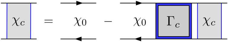
Figure 1: Schematic representation of the Bethe-Salpeter equation in the charge channel (see text).

Inverting Eq. (3) and considering $\bm{\Gamma}_{c}$, $\bm{\chi}_{ph,0}$ and $\bm{\chi}_{c}$ as matrices of the fermionic Matsubara frequencies ($\nu_{n},\nu_{n^{\prime}}$) leads to

$$\bm{\Gamma}_{c}=\beta^{2}\Big{(}[\bm{\chi}_{c}]^{-1}-[\bm{\chi}_{ph,0}]^{-1}\Big{)}.$$ (4)

It is obvious, hence, that all divergences of $\bm{\Gamma}_{c}$ must correspond to a singular $\bm{\chi}_{c}$-matrixSchaefer2016 (typically no divergence is expected in $[\bm{\chi}_{ph,0}]^{-1}$). In fact, analyzing the matrix in its spectral representation, i.e., the basis of its eigenvectors,

$$[\bm{\chi}_{c}]^{-1}_{\nu_{n}\nu_{n^{\prime}}}=\sum_{i}V^{c}_{i}(i\nu_{n^{\prime}})^{\ast}(\lambda_{i})^{-1}V^{c}_{i}(i\nu_{n})\quad,$$ (5)

leads to the one-to-one correspondence of an irreducible vertex divergence to a vanishing eigenvalue ($\lambda_{i=\alpha}\rightarrow 0$) of the matrix $\bm{\chi}_{c}$ in the fermionic frequencies $\nu_{n},\nu_{n^{\prime}}$.

In particular, for a parameter set ($U,T$) close to a divergence, the corresponding eigenvalue will be vanishingly small ($\lambda_{i=\alpha}\approx 0$), leading to a simplified expression for $\bm{\Gamma}_{c}$:

$$\Gamma_{c}^{\nu_{n}\nu_{n^{\prime}}}\sim\beta^{2}{V^{c}_{\alpha}}(i\nu_{n})^{\ast}\lambda_{\alpha}^{-1}V^{c}_{\alpha}(i\nu_{n^{\prime}}).$$ (6)

One sees immediately how in the proximity of a divergence the full frequency structure of $\bm{\Gamma}_{c}$, i.e., its dependence on the fermionic Matsubara frequencies $\nu_{n}$ and $\nu_{n^{\prime}}$, is determinedSchaefer2016 by the non-zero components of the eigenvector $V^{c}_{\alpha}(i\nu_{n})$ associated to the vanishing eigenvalue $\lambda_{\alpha}$. This leads to a distinction of two classes of irreducible vertex divergences, a global one with an eigenvector $V^{c}_{\alpha}(i\nu_{n})\neq 0\,\forall\,\nu_{n}$ and a local one, where only for a finite subset of frequencies $V^{c}_{\alpha}(i\nu_{n})\neq 0$ holds.

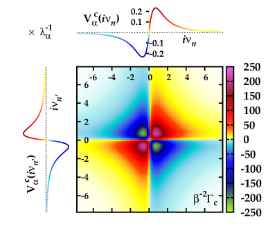
Figure 2: Visualization of the relation between the singular eigenvalues $\lambda_{\alpha}$ and eigenvectors $V^{c}_{\alpha}(i\nu_{n})$ of $\bm{\chi}_{c}$ and the full frequency structure of $\bm{\Gamma}_{c}$ in proximity of a divergence (the specific calculation, shown in the main panel as an example, has been performed for an AIM with $U=3.321444$ and $\beta=40$, yielding $\lambda_{\alpha}=0.00025$). The color of the singular eigenvectors (not related to the color scale of the main plot) highlights the connections to the sign/intensity structure of $\bm{\Gamma}_{c}$ as a function of $\nu_{n}$, $\nu_{n^{\prime}}$, defined by Eq. (6). The values of $\bm{\Gamma}_{c}$ are rescaled by $1/\beta^{2}$ in the main panel for a better readability.

The interplay of eigenvectors, eigenvalues and $\bm{\Gamma}_{c}$ is further discussed in Sec. III.2. Already at this stage, however, we illustrate how the direct relation of Eq. (6) is actually realized in the proximity of a divergence: In Fig. 2 we show a pertinent example of the vertex function computed for a parameter set very close to a divergence, where the lowest eigenvalue $\lambda_{\alpha}$ of $\bm{\chi}_{c}$ is $O(10^{-4})$. In this figure, the full (fermionic) Matsubara frequency dependence ($\nu_{n},\nu_{n^{\prime}}$) of $\bm{\Gamma}_{c}$ is plotted (main panel) together with the eigenvector $V^{c}_{\alpha}(i\nu_{n})$ (both on the left and on top of the main panel) associated to the smallest, almost vanishing, eigenvalue $\lambda_{\alpha}$. It can be easily noticed how in the proximity of a vertex divergence, the frequency structure of $\bm{\Gamma}_{c}$, including the location of the maxima/minima and its signs, is completely controlled by the corresponding frequency dependence of the singular eigenvector $V^{c}_{\alpha}(i\nu_{n})$. The latter encodes, thus, all the essential information about the divergence itself, and will be used in the following for analyzing the evolution of the frequency structure of the vertex function in the proximity of different divergences.

Note that in Sec. III also results for the divergences in the particle-particle up-down channel are shown [$\chi_{pp,\uparrow\downarrow}^{\nu_{n}\nu_{n^{\prime}}}$]. For this channel the same general consideration made here holds, the corresponding Bethe-Salpeter equation can be found in Appendix B of Ref. [Rohringer2012, ] and reads in particle-particle notation

$$\chi_{pp,\uparrow\downarrow}^{\nu_{n}(-\nu_{n^{\prime}})}=-\frac{1}{\beta^{2}}\sum_{{\nu}_{n_{1}}{\nu}_{n_{2}}}\Big{(}\chi_{pp,0}^{\nu_{n}{\nu}_{n_{1}}}-\chi_{pp,\uparrow\downarrow}^{\nu_{n}(-{\nu}_{n_{1}})}\Big{)}\Gamma_{pp,\uparrow\downarrow}^{{\nu}_{n_{1}}{\nu}_{n_{2}}}\chi_{pp,0}^{{\nu}_{n_{2}}\nu_{n^{\prime}}}$$

Let us also briefly comment, at the end of this section, on the degree of two-particle irreducibility of the vertex considered. While the vertex we obtain by the inversion of the Bethe-Salpeter equation in a given channel (e.g. the charge channel) is, per construction, 2PI only in that specific channel, its divergences correspondSchaefer2013 ; Schaefer2016 precisely to the divergences of the fully 2PI vertex function. In this respect, we recall that the vertex divergences found here are not associated to any thermodynamic phase transition, and never appear in the full two-particle scattering amplitude ($F$). Hence, due to the algebraic structure of the parquet equationBickers ; Rohringer2012 , if one of such a divergence occurs, e.g. in $\bm{\Gamma}_{c}$, it has to be compensated by an analogous divergence of the fully 2PI vertex function, in order to preserve the finiteness of $F$ (for more details see [Schaefer2016, ; Rohringer_REV, ]). This has been explicitly verified also for the vertex divergences discussed in the following sections.

We note that the choice of studying the divergences in $\bm{\Gamma}_{c}$, instead of considering the equivalent ones in the fully 2PI vertex, is also suggested by the more direct connection of $\bm{\Gamma}_{c}$ to the LW functional (of which $\bm{\Gamma}_{c}$ represents the second functional derivative) and, hence, to the previously mentioned multivaluedness issuesKozik2015 ; Gunnarsson2017 ; Vucevia2018 .

II.3 Calculations in CT-QMC

We solve the AIM using a continuous-time quantum Monte Carlo (CT-QMC) impurity solver in the hybridization expansionWerner2006 ; Werner2006b . The algorithm is based on a stochastic Monte Carlo sampling of the infinite series expansion of the partition function in terms of the hybridization.

From the stochastic series expansion of the partition function one can construct estimators for the one-particle and two-particle Green’s function and, thus, the generalized susceptibility defined in Eq. (II.2). Extracting the irreducible vertex function from the one- and two-particle Green’s functions, by inverting the corresponding Bethe-Salpeter equation, is a post-processing step to the Monte Carlo measurement, as is the calculation of eigenvalues and eigenvectors of the generalized susceptibility.

Further, we recallSchaefer2016 that for an easier numerical identification of the singular eigenvalues and eigenvectors it is convenient to diagonalize $(\chi_{c}/\chi_{ph,0})^{\nu_{n}\nu_{n^{\prime}}}$ instead of $\chi_{c}^{\nu_{n}\nu_{n^{\prime}}}$. This way it is straightforward to distinguish the vanishing eigenvalues of $\chi_{c}^{\nu_{n}\nu_{n^{\prime}}}$ from the trivial high-frequency eigenvalues ($\propto 1/\nu_{n}^{2}$) and the corresponding eigenvectors. The results are not influenced by this procedure, because the vanishing of an eigenvalue of $\chi_{c}^{\nu_{n}\nu_{n^{\prime}}}$ corresponds to the one of $(\chi_{c}/\chi_{ph,0})^{\nu_{n}\nu_{n^{\prime}}}$ ($\chi_{ph,0}^{\nu_{n}\nu_{n^{\prime}}}$ is not singular). Hence, the specific interaction value for a given temperature where a vertex divergence occurs, i.e. $\widetilde{U}$, is identical. Further, for all cases considered in this work, the numerical difference between the corresponding eigenvectors was found to be negligible. Hence, in the rest of the paper we will consider identical – for all practical purposes – the singular eigenvectors of $(\chi_{c}/\chi_{ph,0})^{\nu_{n}\nu_{n^{\prime}}}$ and $\chi_{c}^{\nu_{n}\nu_{n^{\prime}}}$. The details of the procedure for determining $\widetilde{U}$ for a given temperature, is described in the Appendix C.

For the specific CT-QMC calculations, of the one- and two-particle Green’s function needed in this work, we have employed the w2dynamics softwareParragh2012 . The vertex functions generated by w2dynamics were previously tested against other established codesRibic2017 . Additionally, we have benchmarked the reliability of the impurity solver in computing the vertex divergences of the AIM, against exact diagonalization (ED) results in an intermediate $T$-region, where the discretization of the electronic bath affects the ED procedure only moderately.

For the low temperature calculations, we have quantified the reliability of our results using a Jackknife error analysisJackknife , which is described in the Appendix C.

III Numerical Results

III.1 The T–U diagram

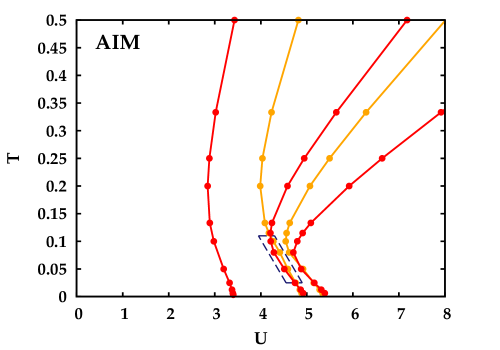
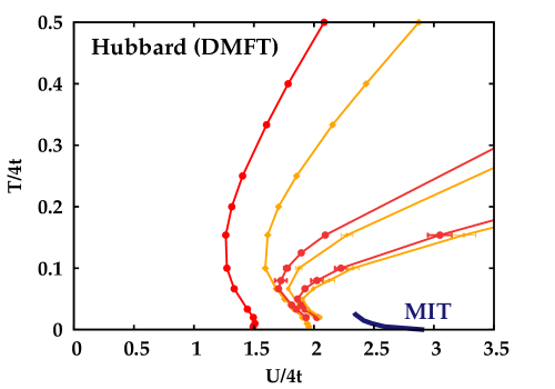
Figure 3: Left panel: $T-U$ diagram of the AIM at half-filling, showing the first divergence lines along which the irreducible vertex functions diverge. For red lines this divergence takes place in the charge channel, $\Gamma_{c}^{\nu_{n}\nu_{n^{\prime}}(\Omega_{n}=0)}$, along the orange lines simultaneous divergences in the charge and the particle-particle up-down channel, $\Gamma_{c}^{\nu_{n}\nu_{n^{\prime}}(\Omega_{n}=0)}$ and $\Gamma_{pp,\uparrow\downarrow}^{\nu_{n}\nu_{n^{\prime}}(\Omega_{n}=0)}$, are observed. The dashed blue box marks the parameter region where the ”atomic” ordering of divergence lines is violated (see text). Right panel: Divergence lines of the half-filled unfrustrated Hubbard model (square lattice dispersion with $4t=1$), solved with DMFT. The lines are plotted with the same color code, the blue solid line represents the Mott-Hubbard MITBluemer_PhD . Re-adapted from Ref. [Schaefer2016, ].

We start to illustrate our numerical results by reporting in the $T$–$U$ diagram of the AIM (Fig. 3 left panel) the first (five) lines along which the two-particle irreducible vertex diverges. These correspond to the interaction values $\widetilde{U}$ at given temperatures $T$, where an eigenvalue of the generalized susceptibility (charge or particle-particle up-down channel) vanishes, see Eq. (4) and Eq. (5). Specifically, the red lines mark irreducible vertex divergences taking place in the charge channel only, while orange lines represent divergences taking place in the charge and the particle-particle up-down channel simultaneously.

Even from the first look at the data, the overall behavior of the divergence lines of the AIM appears qualitatively very similar to the one of the Hubbard model caseSchaefer2013 ; Schaefer2016 , reproduced in the right panel of Fig. 3

In particular, the similarity in the high-temperature/large interaction area of both $T$–$U$ diagrams is not fully unexpected. In fact, here the divergence lines of both models display a rather linear behavior, which is consistent with the insights obtained from the results of the Hubbard atom caseSchaefer2016 . The residual deviations can be ascribed to the fact that the atomic limit condition, i.e., $U$ and $T$ larger than all other energy scales, is not fully complied. In the case of the AIM, only for larger interactions than those shown in the left panel of Fig. 3 ($U\geq D=10$), we recover a purely linear behavior as well as the connection between the position of the divergence line and the inflection point of $\mathrm{Im}\,G(i\nu_{n})$, as expected for the atomic limit (for a more detailed analysis, see Appendix A).

At intermediate temperatures, the divergence lines show a progressively stronger non-linear behavior, starting to bend rightwards. Lowering the temperature further, one reaches the correlated metallic regime. Remarkably, in spite of the differences in the ground states of the two models (there is no MIT in the AIM), even there the results of the AIM and the Hubbard model remain qualitatively very similar. For both models the lines show a ”re-entrance”, i.e. a bending towards higher interaction values, as if the low-temperature intermediate interaction regime were ”protected” against the non-perturbative mechanism originating the irreducible vertex divergences. Particularly remarkable, however, is that finite $\widetilde{U}$ values at $T=0$ are observed in both cases, for the AIM the low-temperature behavior of the first line is investigated in detail in Sec. III.3.

In the framework of the overall similarity discussed above, a specific difference can be seen, however. This is highlighted by the dashed blue box in the left panel of Fig. 3 (see Fig. 4 for a zoom): At intermediate temperatures, the second and third divergence line in the $T$–$U$ diagram of the AIM cross, breaking the typical line-order found in all cases analyzed so far in the literatureSchaefer2013 ; Schaefer2016 ; Gunnarsson2016 ; Ribic2016 ; Gunnarsson2017 (i.e., always an orange line after a red one, before the next red line). The two divergence lines, however, cross again at lower temperatures, restoring the typical line-order. We also observe, that even the fourth and fifth line show such a peculiar crossing, though, to a much smaller extent. To verify the reliability of this observation several tests were performed using exact diagonalization (ED) calculations of the generalized susceptibilityED_Check . As it turns out, our ED analysis (not shown) has confirmed, within the numerical accuracy, the occurrence of such a line crossing.

Although somewhat unexpected and unobserved in preceding studies, the crossing of divergence lines is, however, not in conflict with the most recent theoretical progress made in the analysis of vertex divergences (see Ref. [Gunnarsson2017, ]). In that work, it has been demonstrated that vertex divergences of both kinds are originated by the crossings between different branches of the Luttinger-Ward functional (LWF) of the self-energy. While in the cases considered hithertoGunnarsson2017 ; Vucevia2018 crossings of at most two branches have been reported, it can be logically inferred, that due to the existence of infinite unphysical branches, for other choices of models/parameters (such as in our AIM) crossings among three (or more) branches of the LWF (of which, of course, only one is physical) occursCross . The intersections of two divergence lines observed in our calculations then suggest that this indeed happens for the AIM considered here. It remains to understand, however, why such a situation is, apparently, not realized in the correlated metallic regime of the Hubbard model solved by DMFT.

Finally, as for the theoretical understanding of the low-$T$ regime of the AIM, it is important to estimate the Kondo scale $T_{K}$ and its possible connection to the properties of the irreducible vertex divergences. In Fig. 4 a zoom of the $T$–$U$ diagram of the AIM shown in Fig. 3 is presented together with several estimates for the Kondo temperature $T_{K}$. In particular, the black dotted line represents an analytic estimate valid in the $D\gg U,T$ parameter regimeHewson-precise ($T_{K}=0.4107U(\frac{\Delta}{2U})^{1/2}e^{-\pi U/8\Delta+\pi\Delta/2U}$, where in our AIM: $\Delta=\pi\rho_{0}V^{2}=\pi/5$), while the blue line is determined through the universal scaling of the numerical susceptibility dataKrishna (see Appendix B). We note that the two procedures yield extremely close estimates of $T_{K}$. The Kondo temperature marks however not a phase transition but a smooth crossover. Indeed, the screening processes associated with it become active already at temperatures larger than $T_{K}$. For instance, we see that the temperature below which the effects of the Kondo resonance become visible in the spectrum is $T\lesssim Z\Delta\frac{\pi}{2}$, the half-bandwidth of the central peakHewson . We choose this scale to define the upper border of the corresponding crossover regime (shaded gray area in the $T$–$U$ diagram of Fig. 4). It is quite visible, how the bending of the divergence lines is essentially occurring in this parameter region.

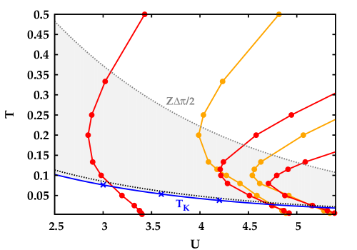
Figure 4: A zoom of the $T$–$U$ diagram of the AIM (left panel Fig. 3) at half-filling is shown. The blue-solid line marks the Kondo temperature ($T_{K}$), estimated from the rescaling of our numerical data for the magnetic susceptibility to the universal function given in Ref. [Krishna, ]. The black-dotted line represents an estimate for $T_{K}$ obtained from an analytic expressionHewson-precise valid in the limit $D\gg U,T$. An additional scale related to the Kondo screening, the half-bandwidth of the $T\rightarrow 0$ Kondo peak ($\frac{\pi}{2}Z\Delta$) Hewson is marked with a gray-dotted line, and is roughly five times larger than $T_{K}$. The light-gray shaded area can be regarded, thus, as the parameter region where the effects of the Kondo screening become visible.

III.2 Classification of the singular eigenvectors

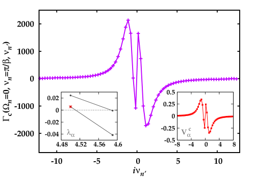
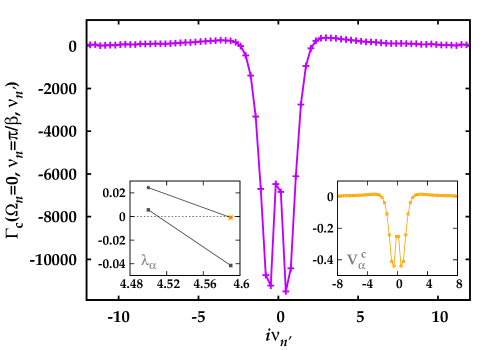
Figure 5: Cuts of the irreducible vertex function in the charge channel, $\Gamma_{c}^{\nu_{n}\nu_{n^{\prime}}(\Omega_{n}=0)}$, for the first Matsubara frequency, $\nu_{1}=\pi/\beta$ at $T=0.05$ and two $U$ values are shown. In the left insets the lowest two eigenvalues of $(\chi_{c}/\chi_{ph,0})^{\nu_{n}\nu_{n^{\prime}}(\Omega_{n}=0)}$ are reported vs. $U$, in the right insets the eigenvector $V_{\alpha}^{c}(i\nu_{n})$ corresponding to the lowest eigenvalue $\lambda_{\alpha}$ is shown as a function of $i\nu_{n}$. Left panel: At $U=4.5$ the lowest eigenvalue is corresponding to the second red divergence line (red dot), hence $V_{\alpha}^{c}(i\nu_{n})$ is antisymmetric. Right panel: For $U=4.59$ the eigenvalue of the first orange line is the smallest (orange dot), $V_{\alpha}^{c}(i\nu_{n})$ is symmetric.

In order to make our study of the vertex divergences in the AIM more quantitative, we proceed with the analysis of the singular eigenvectors in the charge channel, associated to a vanishing eigenvalue of $\chi_{c}^{\nu_{n}\nu_{n^{\prime}}}$ (see Eq. (5)). In fact, as mentioned in Sec. II.2, their frequency structure controls the frequency dependence of $\Gamma_{c}$ in the proximity of – and especially at – a vertex divergence. We note, that for the orange divergence lines, where $\Gamma_{c}$ and $\Gamma_{pp,\uparrow\downarrow}$ diverge simultaneously, the frequency structure of the singular eigenvectors $V^{c}_{\alpha}(i\nu_{n})$ and $V^{pp,\uparrow\downarrow}_{\alpha}(i\nu_{n})$ is found to be identical, which is why $V^{pp,\uparrow\downarrow}_{\alpha}(i\nu_{n})$ will not be shown in the following.

Before showing our numerical results, we discuss some general properties, applicable to a particle-hole and time-reversal symmetric case, like our AIM. In particular, the particle-hole symmetry implies that $\chi_{c}^{\nu_{n}\nu_{n^{\prime}}}$, considered as a matrix of the two fermionic Matsubara frequencies, is a centrosymmetric matrix, i.e., it is invariant under a $\nu_{n}\rightarrow-\nu_{n}$, $\nu_{n^{\prime}}\rightarrow-\nu_{n^{\prime}}$ transformationRohringer2012 ; Rohringer_Diss . A centrosymmetric matrix in Matsubara frequency space has the property that its (non-degenerate) eigenvectors are either symmetric or antisymmetricCentrosymm . Indeed, our results show that eigenvectors associated to red divergence lines are antisymmetric under the transformation $\nu_{n}\rightarrow-\nu_{n}$, whereas orange eigenvectors are symmetric, as it can be seen in the right insets of Fig. 5 and in Fig. 6. The symmetry of the singular eigenvectors is – as expected – well reflected in the frequency structure of the irreducible vertex. As an illustrative example, a cut of the irreducible vertex function in the charge channel, $\Gamma_{c}^{\nu_{n}=\pi T,\nu_{n^{\prime}},\Omega_{n}=0}$ for two values of the interaction $U$ at the same temperature ($T=0.05$) is shown in Fig. 5. In fact, in spite of the proximity between the second red and the first orange divergence line for these parameters, it can be clearly seen how the frequency structure of the vertex function is almost perfectly antisymmetric/symmetric in the case where the lowest eigenvalue corresponds to a red/orange divergence line (left/right panel).

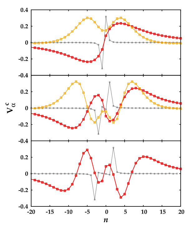
Figure 6: Singular eigenvectors of $(\chi_{c}/\chi_{ph,0})^{\nu_{n}\nu_{n^{\prime}}(\Omega_{n}=0)}$ (numerically equivalent to the ones of $\chi_{c}^{\nu_{n}\nu_{n^{\prime}}(\Omega_{n}=0)}$), corresponding to the five divergence lines (left panel Fig. 3), shown as a function of Matsubara index $n$ for the temperature $T=0.025$. In gray the eigenvectors of the red divergence lines for a higher temperature, $T=0.5$, properly rescaled, are plotted, indicating the broadening of $V^{c}_{\alpha}(i\nu_{n})$ for lower temperatures. Top panel: Eigenvectors of the first red divergence line (red, antisymmetric) and the first orange divergence line (orange, symmetric). Middle (Bottom) panel: Same as top panel, but for the second (third) red and orange (red) divergence line.

After discussing this general feature of the singular eigenvectors, applicable to all particle-hole symmetric models hitherto analyzedSchaefer2016 , we turn to their intriguing evolution with decreasing temperature, and start by going back to Fig. 6. There, eigenvectors corresponding to the five divergence lines (three red, two orange) shown in the left panel of Fig. 3 are compared for the same temperature ($T=0.025$). We further plot properly rescaled eigenvectors corresponding to the red lines at the highest temperature employed in the calculations ($T=0.5$) in gray. The latter show an almost perfect agreement with the atomic limit: Eigenvectors, localized in Matsubara frequency space, which have finite weight almost only at one frequency [$\nu_{n}=(2n+1)\pi T$] equal to the energy scale $\nu^{\ast}$. For example for the first divergence line (top panel) the gray eigenvector displays its by far largest contribution at the first Matsubara frequency ($n=1$).

This specific property of frequency localization characterizing the singular eigenvectors of the red divergence lines (see Sec. II.2) gets lost, however, when reducing the temperature. At $T=0.025$ (red and orange eigenvectors) we note that their frequency decay is even slower than for the singular eigenvectors of the orange lines, which are always associated to ”global” divergences, even in the ALSchaefer2016 . This means, in turn, that also the divergence of $\Gamma_{c}$ is no longer restricted to a finite set of frequencies. Such a ”frequency-broadening” of the red singular eigenvectors at low temperatures was so far only observed in the DMFT solution of the Hubbard modelSchaefer2016 , and seems to be associated with the presence of coherent quasiparticle excitations.

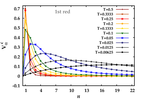
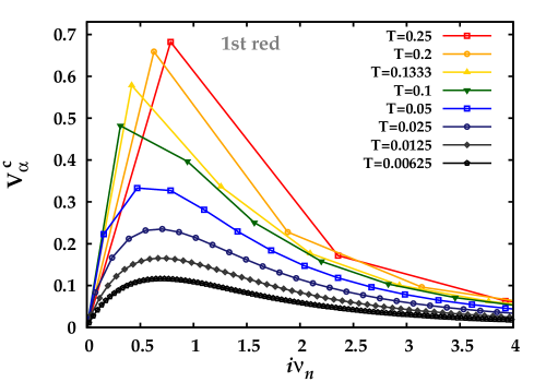
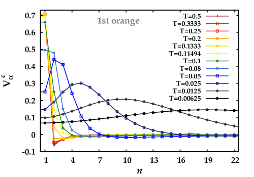
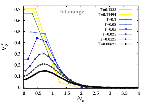
Figure 7: Left top panel: Singular eigenvectors $V^{c}_{\alpha}(i\nu_{n})$ for several temperatures along the first red divergence line, plotted as a function of the Matsubara index $n$. Right top panel: Singular eigenvectors of the left top panel plotted as a function of Matsubara frequency $i\nu_{n}$ instead. Bottom panels: As top panels, but showing the data corresponding to the first orange divergence line.

This general trend is analyzed in detail in Fig. 7: In the left panels the eigenvectors are plotted in terms of the Matsubara index $n$, while in the right panels several $V^{c}_{\alpha}$ for low temperatures are reported as a function of Matsubara frequency $i\nu_{n}$. It can be easily seen, then, that for the eigenvectors corresponding to the first red (upper) and the first orange (lower) divergence line two regimes are distinguishable: ($i$) for $T\gg T_{K}$, the $V^{c}_{\alpha}$ are strongly peaked at a given Matsubara index $n_{\text{max}}$, in perfect agreement with the results of the AL. ($ii$) for $T\lesssim T_{K}$ the maximum contribution of the eigenvector moves to a higher index with decreasing temperature, i.e. to the right (Fig. 7 left panels). Remarkably, one notices instead that, as a function of Matsubara frequency, the maximum contribution of $V^{c}_{\alpha}(i\nu_{n})$ remains localized at a given frequency $i\nu_{n_{\text{max}}}$ in this regime (Fig. 7 right panels).

Finally, it is interesting to analyze in more detail the low-frequency structures of $V^{c}_{\alpha}(i\nu_{n})$, which can be highlighted by comparing the red singular eigenvectors of different lines at the same low temperature, see Fig. 6. In particular, for the eigenvector of the second red divergence line (middle panel of Fig. 6) an additional local maximum and minimum appear at the lowest frequencies, leading to three ”nodes” in their frequency components. In the case of the third red line (bottom panel) $V^{c}_{\alpha}(i\nu_{n})$ has five ”nodes”. Extrapolating the behavior observed for the first three red divergence lines, one expects that the eigenvector of the $n$-th red divergence line will have $2n-1$ ”nodes”. It is also interesting to note, that for the eigenvectors of the first and second red divergence line the respective one or three nodes are also observed in the high-$T$ regime (see the gray eigenvectors). This, however, no longer holds for the eigenvector of the third line.

III.3 Calculations in the low-T regime

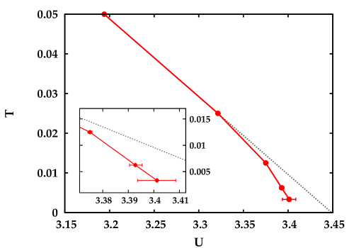
Figure 8: Zoom on the first red divergence line showing the low-$T$ behavior (for $T\ll T_{K}$) which shows, that within the error bars obtained by a Jackknife analysis (see Appendix C) the line bends towards the U axis for $T\rightarrow 0$. Inset: Further zoom on the lowest temperatures, emphasising the growth of the error bar with decreasing temperature.

Before proceeding with the interpretation of our results and their implications, we conclude this section with a detailed analysis of our data in the regime of the lowest temperatures accessible to our algorithm. This is particularly important, because a correct determination of the vertex divergences for $T\rightarrow 0$ is crucial for answering the questions posed in Sec. I.

We start, thus, assessing the numerical accuracy of our results for the first red divergence line in the low-$T$ range ($0.003\overline{3}<T<0.05<T_{K}\sim 0.07$). Our results are shown in Fig. 8, together with the corresponding error bars. The latter were obtained from a Jackknife error analysisJackknife , which is described in detail in the Appendix C. From the error bars in the main plot and the inset of Fig. 8 it can be inferred, that the combined scaling ($\beta^{3}$ of the CT-QMC sampling and $\beta^{2}$ of the Matsubara frequency box of the vertex function for $\Omega_{n}=0$) prohibits us to access temperatures lower than $T=0.003\overline{3}$, therefore not yielding any further informative results about the vertex divergences. However, the numerical precision for $T>0.003\overline{3}$ was sufficient to accurately define the low-$T$ behavior. In fact, we can compare our data with the dotted gray line, showing a linear extrapolation of the divergence line to $T\rightarrow 0$ using the (higher) temperatures $T=0.05$ and $T=0.025$. Even considering the growing error bars, the first divergence line shows a progressive leftwards deviation from the linear extrapolation when reducing the temperature. This is evidently completely inconsistent with an infinite value of $\widetilde{U}$ of the divergence line endpoint for $T\rightarrow 0$.

That the temperatures considered are low enough to allow for a $T\rightarrow 0$ extrapolation is also supported by the behavior of the singular eigenvectors. We discuss here the case for the first red and orange divergence, which is representative for all calculated divergence lines. In fact, for $T\ll T_{K}$ (e.g. for $T\leq 0.025$ for the first divergence) the eigenvectors do not only display a maximum at a $T$-independent value $i\nu_{n_{\text{max}}}$, but as functions of $i\nu_{n}$, they even show a perfect scaling in the whole low-$T$ regime (see Fig. 9). This demonstrates that the low-$T$ frequency structure of the singular eigenvectors, and hence, of the vertex divergences, is completely controlled by an underlying, $T$-independent, function: $\widetilde{V}^{c}_{\alpha}(i\nu)$, such that $V^{c}_{\alpha}(i\nu_{n},T)=f(T)\widetilde{V}^{c}_{\alpha}(i\nu)$. Our numerical data indicates further that $f(T)$ simply represents the conversion factor needed, when taking the $T\rightarrow 0$-limit of the discrete sum of Matsubara frequencies defining the norm of the eigenvector ($\sum_{v_{n}}|V^{c}_{\alpha}(i\nu_{n},T)|^{2}=1$): $f(T)=\sqrt{2\pi T}$. In Fig. 9 the correspondingly rescaled eigenvectors ($=\widetilde{V}^{c}_{\alpha}(i\nu)$) for the first red and orange divergence line are shown. These are extracted from the data for $V^{c}_{\alpha}(i\nu_{n},T)$ by exploiting the low-$T$ scaling relation:

$$\widetilde{V}^{c}_{\alpha}(i\nu)=\frac{{V}^{c}_{\alpha}(i\nu_{n},T)}{f(T)}=\frac{{V}^{c}_{\alpha}(i\nu_{n},T)}{\sqrt{2\pi T}}$$ (7)

In the case of $\widetilde{V}^{c}_{\alpha}(i\nu)$, $i\nu$ represents continuous imaginary frequencies.

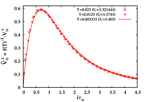
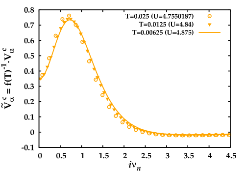
Figure 9: Left panel: Eigenvectors of the first red divergence line for a given temperature multiplied with the inverse of the scaling factor $f(T)$ yielding the eigenvector at $T=0$ governing the frequency structure of the eigenvectors at all temperatures in the $T\ll T_{K}$ regime. Right panel: As left panel, but for the first orange divergence line. Here the minor discrepancies can be ascribed to a stronger $U$ dependence of the singular eigenvectors in comparison to those of the red lines.

IV Discussion and analysis

Our numerical study of the vertex divergences in the AIM presented in the previous sections, and the comparison of the results to the ones of the Hubbard model in DMFT, yield clear-cut answers to several open questions on this subject, which were mentioned at the end of Sec. I.

In particular, the results definitely demonstrate that (i) the MIT does not represent the essential ingredient to induce vertex divergences (as well as the associated non-perturbative manifestations). This is proven by the similarity of the low-$T$ behavior of the vertex divergence lines in the Hubbard model and the AIM, ending in both cases at finite $U$ values in the limit $T\rightarrow 0$, although no MIT occurs in the ground state of the latter. We must conclude, hence, that the occurrence of a MIT can represent a sufficient, but not a necessary, condition to observe vertex divergences. In this respect we recall that in the phase diagrams of the Hubbard/FK models the MIT cannot be reached (from the non-interacting or the high-$T$ perturbative region) without crossing (at least) one divergence line: Only in this somewhat more limited context, the vertex divergences can be regarded as ”precursors” of the MIT, as originally proposedSchaefer2013 .

The picture emerging from our AIM data does not contradict, however, the physical considerations made in Ref. [Gunnarsson2016, ; Gunnarsson2017, ], where one could relate the suppression of the charge susceptibilityGunnarsson2017 , driven by the formation of a local magnetic momentGunnarNote , to the onset of the divergences. The same physical mechanism can also induce, depending on the model, the appearance of a MIT. This scenario would be, thus, coherent with our numerical finding of divergence lines without a MIT.

At the same time, the origin of the rather striking similarity between the low-$T$ curvature of the divergence lines and the MIT in the DMFT phase diagram of the Hubbard model can be further rationalized, as we will discuss below, in terms of the relation to $T_{K}$.

Further, (ii) the observation of an overall qualitatively similar $T$–$U$ diagram (down to very low $T$) rules out the proposed explanation of the line re-entrance shape in terms of the so called ”ring-scenario”Schaefer2016 . This proposed scenario represents a simple generalization of the theoretical framework applicable at high $T$ and large $U$. We recallSchaefer2016 that, in the latter regime, the existence of infinitely many divergence lines could be interpreted as a direct manifestation of an underlying energy scale $\nu^{*}$ in the Matsubara frequency space: A divergence occurs whenever a Matsubara frequency ($\nu_{n}=\frac{\pi}{\beta}(2n+1)$) equals $\nu^{*}$. While it was already made clear in previous studiesSchaefer2016 , that this high-$T$ explanation does not work at low-$T$, a simple generalization was proposed: At low-$T$ two underlying energy scales might control the vertex divergences. This idea would have matched well previous results showing that in the DMFT solution of the Hubbard model (for roughly the same interaction values where the divergences occur) two energy scales $\omega_{FL}$ and $\omega_{CP}$ appear in the low-energy sectorByzuk2007 , where the renormalized quasiparticle excitations of the systems are defined. From a merely theoretical viewpoint, the separation of low-energy scales can be ascribedHeld2013 to the self-consistent renormalization of the electronic bath of the auxiliary AIM of DMFT in the correlated metallic regime. This has also important observable consequences, like the emergence of kinks in the spectral functionsByzuk2007 and the specific heatToschi2009 of the Hubbard model. In the perspective of the vertex divergences, the emergence of two energy scales on the real axis would correspond to a situation (referred to as “ring-scenario”) where the perturbative physics is preserved not only – as usual – at high energy (for $\omega>\omega_{CP}$), but also in the lowest frequency Fermi-Liquid $(FL)$ regime (for $\omega<\omega_{FL}$), for a schematic representation see Fig. 10. The non-perturbative effects, instead, would appear first at intermediate energies, i.e., for $\omega_{FL}<\omega<\omega_{CP}$, and reach the Fermi level, only at the MIT.

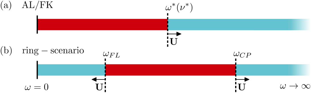
Figure 10: Schematic representation of the energy scale(s) controlling the border(s) of the perturbative/non-perturbative regimes, (a): in the AL/FK case, which is relevant for the large $T$ and $U$ limit of the AIM and the DMFT solution of the Hubbard model, (b): for the ”ring-scenario” which was proposed in Ref. [Schaefer2016, ], for the Hubbard model in the correlated metallic regime (see text). Note that for the AIM with a large bandwidth, as studied here, only one energy scale exists.

The existence of two scales could be indeed reflected in the observed more complex non-local structure of the singular eigenvectors in Matsubara space. Moreover, this interpretation would also have the appealing advantages of providing a one-to-one correspondence of the vertex divergences to physical observables (the kinks), and, at the same time, of avoiding the necessity to deal with a Fermi-Liquid ground state, of intrinsic non-perturbative nature.

Our finding of qualitatively similar divergence lines, also in the low-$T$ area of the $T$–$U$ diagram of the AIM, however, makes a general validity of the proposed “ring-scenario” very unlikely: In our AIM with a fixed and large conduction electron bandwidth, the intrinsic origin of the separation of energy scales (i.e., the self-consistent renormalization of the electronic bath) is missing, see the discussion in Ref. [Held2013, ,Kainz2012, ].

As a consequence, from a theoretical point of view, one will indeed face the challenge of reconciling the observation of well defined Fermi-Liquid properties at low-energies with the evident breakdown of perturbation theory marked by the multiple divergence lines. In other words, it will be necessary to describe and fully understand the emergence of an intrinsically non-perturbative Fermi-Liquid phase.

From a more physical point of view, the similarity of the divergence lines in the Hubbard model and the AIM also excludes a direct connection of the divergences to the kinks in the self-energy, which are presentByzuk2007 ; Toschi2010 and absentKainz2012 ; Held2013 in the two respective models. Note however, that the kinks in the DMFT solution of the Hubbard model are also related to the Kondo temperatureHeld2013 , so there might be an indirect connection as for the bending of the divergence lines around $T_{K}$, see (iv).

(iii) The presence of several distinct intersections of the divergence lines with the $T=0$ axis poses the question as to whether irreducible vertex divergences occur also on the real frequency axis. In fact, this behavior is radically different from the one found in the FK modelSchaefer2016 ; Janis2014 ; Ribic2016 . In the latter case, all divergences lines accumulate at $T=0$ for a non-zero interaction valueSchaefer2016 ; Ribic2016 ($U=D/\sqrt{2}$), which corresponds to the unique vertex divergence on the real frequency axisSchaefer2016 ; Janis2014 . The low-$T$ spread displayed by the divergence lines of the AIM is, thus, fully incompatible with the simpler FK scenario of a single divergence point of the vertex in real-frequency. In this respect, important insight is provided by the analysis of the temperature evolution of the singular eigenvectors $V^{c}_{\alpha}(i\nu_{n})$ for the different lines, especially in the low-$T$ regime where their behavior can be fully described by a rigid scaling (see Sec. III.3 and Fig. 9). In fact, close to the divergence, $\Gamma_{c}$ can be approximated as in Eq. (6). The scaling properties of the eigenvectors, combined with the different (odd/even) symmetries (under $\nu_{n}\rightarrow-\nu_{n}$) of the eigenvectors corresponding to the red/orange divergences, provide a strong indication that real-frequency divergences in the limit of zero frequencies, i.e. $i\Omega_{n}=0,i\nu_{n},i\nu_{n^{\prime}}\rightarrow 0$, will appear at the endpoints of all orange lines. This is due to the fact that for the rescaled eigenvectors of orange divergence lines the value of the lowest frequency component of the singular eigenvector is finite and non-zero in the $T\rightarrow 0$ limit ($\widetilde{V}^{c}_{\alpha}(i\nu=0)\neq 0$, see Sec. III.3 and Fig. 9). On the contrary, the vanishing of $\widetilde{V}^{c}_{\alpha}(i\nu=0)$ for red divergences, which is enforced by the odd symmetry of the eigenvector, suggests the absence of similar real-frequency divergences as for the orange endpoints. This would represent a further, major differentiation between the two kinds of divergences, as only the orange ones would be mirrored by corresponding divergences at the origin of the real-frequency axis at the $T=0$ endpoints. Of course, our analysis can not exclude, that the real frequency vertex functions might display additional divergences at finite non-zero frequencies.

(iv) The precise determination of the Kondo temperature in the $T$–$U$ diagram of the AIM we considered (Fig. 4) provides novel insights into the problem of the vertex divergences in the correlated metallic regime. First, as we briefly mentioned in Sec. III, the relatively featureless and smooth behavior of all divergence lines for $T<T_{K}$ indicates that unexpected bending below the lowest temperature where the QMC calculations of the impurity vertex functions are feasible, is highly improbable and also incompatible with the perfect scaling of the singular eigenvectors discussed in Sec. III.3. This represents an important, physics-based argument supporting all low-$T$ results and considerations discussed before. Second, we must recall that the Kondo screening in the AIM is not taking place as a sharp transition. On the contrary, it is known that the impurity magnetic moment screening starts to become progressively effective at temperature larger than $T_{K}$. In fact, considering the low-energy spectral properties of the impurity site, a natural estimate of the crossover temperature, leads to values more than five times larger than the “standard” $T_{K}$ (see Sec. III.1). This is relevant for the interpretation of our results, as the bending of the divergence lines, and in particular their re-entrance behavior, is taking place in this crossover regime. Consistently, in the same parameter region, the qualitative change in the structure of the eigenvectors for the red lines (and of the corresponding divergence of $\Gamma_{c}$ from localized to non-localized in frequency space) takes place. The emerging scenario for the breakdown of perturbation expansion in the AIM is, thus, the following: Vertex divergences with a relatively simple structure (straight linear behavior of all divergence lines, fully localized eigenvectors, etc.) are associated to the formation of a local moment, and to the related net separation of energy scales, marked by a spectral gap between the Hubbard bands. This agrees with our understanding in the ALSchaefer2013 ; Rohringer_Diss ; Schaefer2016 ; Rohringer_AL .

The progressive Kondo screening occurring by lowering $T$ towards $T_{K}$ is responsible for the gradual, but important deviations from this “simpler” divergent behavior. In particular, it is interesting to note that the screening of the local moment appears, to some extent, to ”counter” the breakdown of the perturbation expansion (low-$T$ re-entrance) of the lines. This effect, however, is only partial, as the divergence lines for $T<T_{K}$ are not bending up to $U=\infty$, but rather display multiple (presumably infinite) endpoints on the $T=0$ axis.

(v) From the numerical results obtained for the AIM and from the considerations made hitherto, it is possible to formulate specific, though somewhat heuristic, predictions for the structure of the divergence lines in the DMFT solution of the Hubbard model. In particular, we will focus on the most interesting regime of the coexistence region surrounding the Mott-Hubbard MIT. In fact, due to the considerable accumulations of vertex divergences close to the MIT, no detailed study of the irreducible vertex functions in this parameter region has been performed so far.

The starting point for our prediction is the connection discussed above (iv), between the Kondo screening, controlled by $T_{K}$, and the bending of the divergence lines. Further, it is also important that for $T<T_{K}$ each of the (infinitely) many lines smoothly continues down to their respective finite endpoint on the $T=0$ axis (iii). In fact, a converged DMFT solution is defined through the self-consistently determined electronic bath of the auxiliary AIM. This means that the AIM of a given DMFT solution would be characterized by a $T_{K}$ depending not only on $U$ but also on $T$, $n$, etc. Such an “effective” $T_{K}^{\text{DMFT}}(U,T)$ becomes zero at the Mott-Hubbard MIT at $T=0,U\rightarrow U_{c2}$. This suggests that, the divergence lines appearing in the $T<T_{K}$ part of the whole $T$-$U$ parameter space of the AIM will be squeezed in the region $U<U_{c2}$ of the DMFT solution of the Hubbard model. This will evidently result in an accumulation of divergence lines close to $U_{c2}$. For $T\neq 0$, instead, one will cross, by increasing $U$, a first order MIT where a discontinuity of the physical properties occurs. Such a discontinuity affects, among other observables like the double occupancy or the kinetic energy, also the self-consistently determined electronic bath of the auxiliary AIM. Hence, one must expect that the number of negative eigenvalues of $\chi_{c}$ (and thus, of divergences lines already crossed) will be different on the two sides of the transition, except for $T=0$ and at the critical endpoint where the MIT is continuous. More specifically, we recall that the Mott insulating phase is characterized by an essentially unscreened local moment. As a consequence, on the insulating side of the MIT we will observe only very minor corrections w.r.t. the divergence lines computed in the AL (straight lines with frequency localized red divergences, etc.). On the metallic side of the MIT, instead, the electronic bath is associated with a finite $T_{K}^{\text{DMFT}}(T,U)$, and, thus, the screening effect, partially mitigating the vertex divergences, will be at work. As a result, for a fixed $T\neq 0$ one would find here a fewer number of negative eigenvalues (and, hence, of divergences lines) than on the insulating side. Eventually, for low-enough $T\sim T_{K}^{\text{DMFT}}(U,T)$, the divergence lines on the metallic side will show the typical bending behavior, and display very frequency delocalized eigenvectors.

V Conclusion and Outlook

In this work we have studied the divergences of the irreducible vertex functions occurring in an Anderson impurity model with a fixed electronic bath, aiming at gaining novel insights about the breakdown of many-body perturbation theory in correlated metallic systems. In fact, the numerical solution of the AIM, computed at high accuracy in CT-QMC, fully captures the physics of low-temperature quasi-particle excitations, as those observed in correlated metals. It avoids, however, the additional complication of a self-consistent adjustment of the electronic bath required by DMFT calculations. Hence, the AIM represents a fundamental test bed to address several open issues posed in the literature, about the different non-perturbative manifestations in quantum many-body theory.

Indeed, our study could clarify a set of relevant questions about the interpretation and the consequences of the divergences of the two-particle irreducible vertex functions. In particular, our results rule out that the Mott-Hubbard transition plays a crucial role as the origin of the multiple divergence lines. This limits the previously proposed interpretationSchaefer2013 of the vertex divergences as “precursors” of the MIT in the sense of a necessary condition for vertex divergences to occur, consistently with the physical interpretation presented in Refs. [Gunnarsson2016, ; Gunnarsson2017, ]. By a thorough analysis of the low-temperature sector, we could ascribe, at the same time, important characteristics of the vertex divergences, such as their structure in Matsubara frequency space and the re-entrance of the divergences line, to the screening processes of the local magnetic moment occurring when approaching $T_{K}$. Moreover, our data for $T\ll T_{K}$ has unveiled a perfect scaling of the singular eigenvectors, allowing us to extrapolate the $T=0$ behavior of the vertex divergences on the real-frequency axis. Finally, exploiting the insights gained from the low-$T$ analysis, we could propose a heuristic prediction about the vertex divergences in the particularly relevant case of the coexistence region in the DMFT phase diagram of the Hubbard model.

Having clarified important properties of the vertex divergences in the correlated metallic phase (partly with an unexpected outcome which corrected previously made assumptions) our work also demonstrates how valuable studies are, where the many-body correlation effects are realized in the most fundamental fashion. This suggests future extensions of this work, by considering systems with embedded clusters of impurities, to investigate the role played by short-range correlations in the breakdown of the quantum many-body perturbation expansion.

Appendix

Appendix A: The atomic limit and the inflection point of $\bm{\mathrm{Im}\,G(i\nu_{n})$}$

As mentioned in Sec. I, in the case of the atomic limit, the inflection point of $\mathrm{Im}\,G(i\nu_{n})$ is foundRohringer_AL at the frequency $\nu_{n}=\nu^{\ast}$, i.e. the energy scale which is also governing the position of the divergence lines and the frequency structure of the localized singular eigenvectors corresponding to red divergence lines. As we briefly discuss in Sec. III.1, this connection is also found for the Anderson impurity model, in the regime of high-$T$ and large interaction. The results are shown explicitly in Fig. 11 of this Appendix, where the rescaled $\mathrm{Im}\,G(i\nu_{n})$ is compared to $\partial^{2}\mathrm{Im}\,G(i\nu_{n})=\frac{\partial^{2}\mathrm{Im}\,G(i\nu_{n})}{\partial\nu_{n}^{2}}$ for the third red divergence line. Note that in the simple method used to compute the second derivative of $\mathrm{Im}\,G(i\nu_{n})$, namely finite differences, there is no data for the first frequency. For $T=0.5$ (see Fig. 11a), it is evident that the inflection point is located at the third Matsubara frequency, which agrees with the atomic limit description. With decreasing temperatures, the inflection point moves from the third frequency towards lower frequencies, which is visible in Fig. 11b, where it is found between the second and third frequency for $T=0.3\bar{3}$. Although the divergence line shows still a rather linear behavior (see main part, Fig. 3), the inflection point completely disappears for $T=0.2$ (see Fig. 11c).

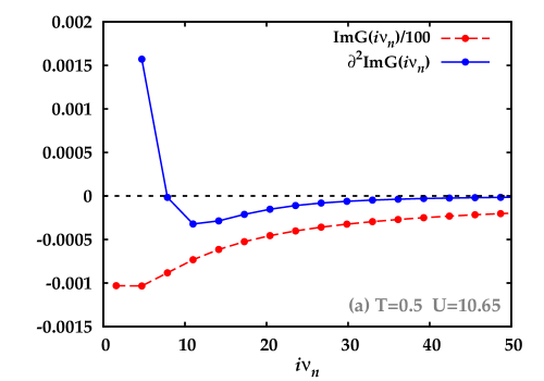
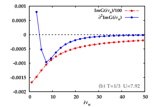
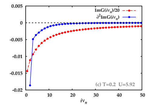
Figure 11: Comparison of $\mathrm{Im}\,G(i\nu_{n})$ (rescaled by a proper factor) and $\partial^{2}\mathrm{Im}\,G(i\nu_{n})=\frac{\partial^{2}\mathrm{Im}\,G(i\nu_{n})}{\partial\nu_{n}^{2}}$ for three different temperatures along the third red divergence line of the AIM.

Appendix B: The numerical extraction of the Kondo temperature $\bm{T_{K}}$

To extract the Kondo temperature $T_{K}$ numerically the static local magnetic susceptibility of the impurity $\chi_{s}(i\Omega_{n}=0)$ has been calculated by integrating $\chi_{s}(\tau)=g^{2}\langle S_{z}(\tau)S_{z}(0)\rangle$, with $g=2$ (computed with w2dynamics) over the interval $[0,\beta]$.

$$\chi_{s}(i\Omega_{n}=0)=\int\limits_{0}^{\beta}\chi_{s}(\tau)$$ (8)

which corresponds to its Fourier transform for $i\Omega_{n}=0$. The data for $\chi_{s}(i\Omega_{n}=0)$ has been computed for several $T$, and then compared to the universal result for $\frac{T\chi_{s}(T)}{(g\mu_{B})^{2}}$, computed for the spin-$\frac{1}{2}$ Kondo Hamiltonian in Ref. [Krishna, ] (cf. also Ref. [Wilson_kondo, ]), where $\mu_{B}$ is the Bohr magneton. Plotted as a function of $log(T/T_{K})$ the Kondo temperature can thus be obtained with high precision by shifting the numerical data for $T\chi_{s}(i\Omega_{n}=0)$ onto the universal result (on a logarithmic $T$-scale). For the case of $U=4.2$ the shifted results are shown in Fig. 12. The data for $T_{K}$ obtained through this procedure are the blue crosses reported in Fig. 4 of the main paper.

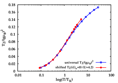
Figure 12: The shifted data for $T\chi_{s}(\omega=0)$ for several temperatures at $U=4.2$, compared to the universal result for $T\chi_{s}(T)$ (see Ref. [Krishna, ]).

Appendix C: The determination of $\bm{\widetilde{U}}$ and the associated error bars

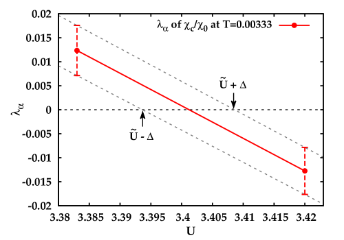
Figure 13: The singular eigenvalue $\lambda_{\alpha}$ of $(\chi_{c}/\chi_{ph,0})^{\nu_{n}\nu_{n^{\prime}}\Omega=0}$ for $T=0.003\bar{3}$ and two different $U$ values ($3.383$, $3.42$) is shown. A linear interpolation is used for the determination of $\widetilde{U}$ (red solid line). The Jackknife error analysis provided error bars for the two results for $\lambda_{\alpha}$ (red dashed), which are, then, used to estimate the error bar of $\widetilde{U}$ (gray dashed lines).

To estimate $\widetilde{U}$ for a given temperature at least two separate calculations of $\chi_{c}^{\nu_{n}\nu_{n^{\prime}}\Omega_{n}=0}$ are necessary. As an example of the procedure, we show the case of the first divergence line for $T=1/300\approx 0.00333$. For this case the smallest eigenvalue of $(\chi_{c}/\chi_{ph,0})^{\nu_{n}\nu_{n^{\prime}}}$ (see Sec. II.3) is plotted as a function of $U$, see Fig. 13. This, in turn, allows us to adopt an interpolation or extrapolation procedure for an estimation of $\widetilde{U}$, depending on whether we find two eigenvalues with different signs or not. In the following a bisection procedure is used until $\widetilde{U}$ is known to the desired accuracy for the given temperature. In the calculations shown throughout this work, we have performed calculations until we reached an interval in $U$ of the order of $\mathcal{O}(10^{-1})$ to $\mathcal{O}(10^{-3})$. For the first line and high-$T$ the coarser interval was used, for the subsequent lines a more refined interval was employed, as well as for the low-$T$ results of all lines. Each calculation was performed on the Vienna Scientific Cluster (VSC3) using about $10.000$ to $15.000$ CPU hours, in the case of the low-$T$ calculations $25.000$ ($\beta=160$) or $50.000$ ($\beta=300$) CPU hours were used.

Finally, to estimate the error bars of the interaction values $\widetilde{U}$ it is necessary to extract, first, the error of the eigenvalues of $(\chi_{c}/\chi_{ph,0})^{\nu_{n}\nu_{n^{\prime}}\Omega_{n}=0}$. To this end a $(n-1)$ Jackknife methodJackknife was used. Specifically, with the same CPU hours used for the calculations discussed above, $25$ bins were produced. From these $25$ different results for $(\chi_{c}/\chi_{ph,0})^{\nu_{n}\nu_{n^{\prime}}\Omega_{n}=0}$ $26$ eigenvalues were produced, according to the ($n-1$) Jackknife methodJackknife , which also provides an expression for the standard deviation. As a last step, the intersection points of the interpolation of the maximum and minimum error of the eigenvalues and zero, were used as an estimate for the error bar of $\widetilde{U}$ for a given $T$. This procedure is also shown explicitly in Fig. 13.

References

- (1) A. Georges, G. Kotliar, W. Krauth, and M. Rozenberg, Rev. Mod. Phys. 68, 13 (1996).
- (2) T. Maier, M. Jarrell, T. Pruschke, and M. H. Hettler, Rev. Mod. Phys. 77, 1027 (2005).
- (3) G. Rohringer, H. Hafermann, A. Toschi, A. A. Katanin, A. E. Antipov, M. I. Katsnelson, A. I. Lichtenstein, A. N. Rubtsov, and K. Held, Rev. Mod. Phys. 90, 025003 (2018).
- (4) A. Toschi, A. A. Katanin, and K. Held, Phys. Rev. B 75, 045118 (2007).
- (5) A. N. Rubtsov, M. I. Katsnelson, and A. I. Lichtenstein, Phys. Rev. B 77, 033101 (2008).
- (6) A. N. Rubtsov, M. I. Katsnelson, and A. I. Lichtenstein, Ann. Phys. (NY) 327, 1320 (2012).
- (7) G. Rohringer, A. Toschi, H. Hafermann, K. Held, V. I. Anisimov, and A. A. Katanin, Phys. Rev. B 88, 115112 (2013).
- (8) C. Taranto, S. Andergassen, J. Bauer, K. Held, A. A. Katanin, W. Metzner, G. Rohringer, and A. Toschi, Phys. Rev. Lett. 112, 196402 (2014); N. Wentzell, C. Taranto, A. Katanin, A. Toschi, and S. Andergassen, Phys. Rev. B 91, 045120 (2015).
- (9) T. Ayral, and O. Parcollet, Phys. Rev. B 92, 115109 (2015).
- (10) M. Kitatani, N. Tsuji, and H. Aoki, Phys. Rev. B 92, 085104 (2015).
- (11) T. Ayral, and O. Parcollet, Phys. Rev. B 94, 075159 (2016).
- (12) T. Schäfer, G. Rohringer, O. Gunnarsson, S. Ciuchi, G. Sangiovanni, and A. Toschi, Phys. Rev. Lett. 110, 246405 (2013).
- (13) E. Kozik, M. Ferrero, and A. Georges, Phys. Rev. Lett. 114, 156402 (2015).
- (14) T. Schäfer, S. Ciuchi, M. Wallerberger, P. Thunström, O. Gunnarsson, G. Sangiovanni, G. Rohringer, and A. Toschi, Phys. Rev. B 94, 235108 (2016).
- (15) V. Janiš and V. Pokorny, Phys. Rev. B 90, 045143 (2014).
- (16) T. Ribic, G. Rohringer, and K. Held, Phys. Rev. B 93, 195105 (2016).
- (17) G. Rohringer, PhD Thesis, Technische Universität Wien (2014).
- (18) J. Vucicevic, N. Wentzell, M. Ferrero, O. Parcollet, Phys. Rev. B, 97, 125141 (2018).
- (19) A. Stan, P. Romaniello, S. Rigamonti, L Reining and J.A. Berger New J. of Physics 17 093045 (2015).
- (20) J. Hubbard, Proc. Roy. Soc. London A 276, 238 (1963); M. C. Gutzwiller, Phys. Rev. Lett. 10, 159 (1963); J. Kanamori, Progr. Theor. Phy. 30, 275 (1963).
- (21) G. Lani, P. Romaniello, and L. Reining, New J. Phys. 14, 013056 (2012).
- (22) J. A. Berger, P. Romaniello, F. Tandetzky, B. S. Mendoza, C. Brouder, and L. Reining, New J. Phys. 16, 113025 (2014).
- (23) O. Gunnarsson, T. Schäfer, J. P. F. LeBlanc, J. Merino, G. Sangiovanni, G. Rohringer, and A. Toschi Phys. Rev. B 93, 245102 (2016).
- (24) R. Rossi and F. Werner, J. Phys. A 48, 485202 (2015).
- (25) H. Keiter, T. Leuders, Europhys. Lett. 49, 801 (2000).
- (26) O. Gunnarsson, G. Rohringer, T. Schäfer, G. Sangiovanni, and A. Toschi, Phys. Rev. Lett. 119, 056402 (2017).
- (27) For a review, see, e.g., N. E. Bickers, Int. J. Mod. Phys. B 5, 253 (1991) and in Theoretical Methods for Strongly Correlated Electrons, edited by D. Senechal, A. Tremblay, and C. Bourbonnais (Springer-Verlag, New York, 2004), chapter 6.
- (28) S. X. Yang, H. Fotso, J. Liu, T. A. Maier, K. Tomko, E. F. D’Azevedo, R. T. Scalettar, T. Pruschke, and M. Jarrell, Phys. Rev. E 80, 046706 (2009).
- (29) Ka-Ming Tam, H. Fotso, S.-X. Yang, Tae-Woo Lee, J. Moreno, J. Ramanujam, and M. Jarrell Phys. Rev. E 87, 013311 (2013).
- (30) Gang Li, A. Kauch, P. Pudleiner, and K. Held, arXiv:1708.07457.
- (31) A. Toschi, G. Rohringer, A. Katanin, and K. Held, Ann. Phys. 523, 698 (2011).
- (32) A. Galler, P. Thunström, P. Gunacker, J. M. Tomczak, and K. Held, Phys. Rev. B 95, 115107 (2017).
- (33) C. Slezak, M. Jarrell, Th. Maier, and J. Deisz, J. Phys.: Condens. Matter 21, 435604 (2009).
- (34) W. Tarantino, P. Romaniello, J. A. Berger, and L. Reining, Phys. Rev. B 96, 045124 (2017).
- (35) For the diagrammatic methods based on the inversion of the Bethe Salpeter equations, such as the ladder version of DAKatanin2009 ; Rohringer2016 ; Galler2017 and the multiscaleSlezak2009 approach, the divergences of the corresponding 2PI DMFT vertex, on which the algorithmic are based, could be completely bypassed by re-expressing the corresponding ladders in terms of the 1PI DMFT vertex functions (see Rohringer_Diss ; Rohringer_REV for details). The problems originated by the multivaluedness of the LWF might be possbily addressedEder2015 ; Rossi2016 ; Tarantino2017 with appropriate restrictionsPotthoff2006 of the mathematical space of the and/or with specific treatments of the convergence criteria. For the moment, it is not at all clear, instead, whether (or to what extent) the effect of the divergences can be circumvented in all the algorithm exploiting parquet solversYang2009 ; Tam2013 ; Li2017 beyond the perturbative regime, such as e.g., in DAValli2015 ; Li2016 , QUADRILEXQUADRILEX or the parquet decomposition procedureGunnarsson2016 .
- (36) A. Katanin, A. Toschi, and K. Held, Phys. Rev. B 80, 075104 (2009).
- (37) G. Rohringer, and A. Toschi, Phys. Rev. B 94, 125144 (2016).
- (38) R. Eder, arXiv:1407.6599.
- (39) R. Rossi, F. Werner, N. Prokof’ev, and B. Svistunov, Phys. Rev. B 93, 161102(R) (2016).
- (40) M. Potthoff, Condens. Matt. Phys. 9, 3(47), 557-567 (2006).
- (41) A. Valli, T. Schäfer, P. Thunström, G. Rohringer, S. Andergassen, G. Sangiovanni, K. Held, and A. Toschi, Phys. Rev. B 91, 115115 (2015).
- (42) Gang Li, N. Wentzell, P. Pudleiner, P. Thunström, and K. Held, Phys. Rev. B 93, 165103 (2016).
- (43) N. F. Mott, Rev. Mod. Phys. 40, 677 (1968); Metal-Insulator Transitions (Taylor & Francis, London, 1990); F. Gebhard, The Mott Metal-Insulator Transition (Springer, Berlin, 1997).
- (44) K. Byczuk, M. Kollar, K. Held, Y.-F. Yang, I. A. Nekrasov, T. Pruschke, and D. Vollhardt, Nat. Phys. 3, 168 (2007).
- (45) K. Held, R. Peters, and A. Toschi Phys. Rev. Lett. 110, 246402 (2013).
- (46) A. Toschi, M. Capone, C. Castellani, and K. Held, Phys. Rev. Lett. 102, 076402 (2009).
- (47) A. Toschi, M. Capone, C. Castellani, and K. Held, J. Phys. Conf. Ser. 200, 012207 (2010).
- (48) L. Schwartz, and E. Siggia, Phys. Rev. B, 5 383 (1972).
- (49) R. Vlaming, and D. Vollhardt, Phys. Rev. B, 45 4637 (1992).
- (50) P. Soven Phys. Rev. 156, 809 (1967); for a review see, e.g. F. Yonezawa, K. Morigaki, Suppl. Prog. Theor. Phys., 53, 1 (1973).
- (51) P. Thunström, O. Gunnarsson, S. Ciuchi, and G. Rohringer, arXiv:1805.00989.
- (52) P. W. Anderson, Phys. Rev. 124, 41 (1961).
- (53) In the DMFT study of Ref. [Byzuk2007, ] the two scales and define respectively the region of applicability of the Fermi Liquid description () and the size of the central peak in the spectral function () in the correlated metallic region before the Mott transition.
- (54) J. Kondo, Progress of Theoretical Physics 32, 37 (1964).
- (55) G. Rohringer, A. Valli, and A. Toschi, Phys. Rev. B, 86 125114 (2012).
- (56) N. Wentzell, Gang Li, A. Tagliavini, C. Taranto, G. Rohringer, K. Held, A. Toschi, and S. Andergassen, arXiv:1610.06520.
- (57) A. Tagliavini, S. Hummel, N. Wentzell, S. Andergassen, A. Toschi, and G. Rohringer, Phys. Rev. B 97, 235140 (2018).
- (58) This is connected to the particle-particle one by a mere frequency shiftSchaefer2016 ; Rohringer_Diss ; Rohringer2012 [].
- (59) P. Werner, and A. J. Millis, Phys. Rev. B 74, 155107 (2006).
- (60) P. Werner, A. Comanac, L. de’ Medici, M. Troyer, and A. J. Millis, Phys. Rev. Lett. 97, 076405 (2006).
- (61) N. Parragh, A. Toschi, K. Held, and G. Sangiovanni, Phys. Rev. B 86, 155158 (2012).
- (62) T. Ribic, P. Gunacker, S. Iskakov, M. Wallerberger, G. Rohringer, A. N. Rubtsov, E. Gull, and, K. Held, arXiv:1710.00648.
- (63) B. Efron, C. Stein, Ann. Statist. 9, 586 (1981).
- (64) N. Blümer, Ph.D Thesis, Universität Augsburg, 2003.
- (65) We have used the implementation described in the Appendix of Ref. [DGA, ] with and .
- (66) In fact, the calculations of Ref. [Gunnarsson2017, ] have indeed shown the existence of several crossings between two unphysical branches of the LWF in the case of the atomic limit. Thus, it is easy to imagine that by changing models or modifying the parameters one of these crossings can touch the physical branch, leading to the situation observed in our – diagram for the AIM.
- (67) See, Eq. (6.109) and ff. at p. 165-166 of Chp. 6.7 in Ref. [Hewson, ].
- (68) H. R. Krishna-murthy, J. W. Wilkins, and K. G. Wilson, Phys. Rev. B 21, 1003 (1980).
- (69) A.C. Hewson, The Kondo Problem to Heavy Fermions, Cambridge University Press (1993).
- (70) I. T. Abu-Jeib, Canadian Applied Mathematics Quarterly 10, 429 (2002).
- (71) As discussed in Ref. [Gunnarsson2016, ], the tendency towards a local moment could be interpreted, to some extent, as the formation of a ”bound state”. Note also that, in the case of cluster calculationsGunnarsson2016 , the formation of an RVB state plays the role of the local moment formation.
- (72) A. Kainz, A. Toschi, R. Peters, and K. Held, Phys. Rev. B 86, 195110 (2012).
- (73) K. G. Wilson, Rev. Mod. Phys. 47, 773 (1975).