Static dilaton space-time parameters from frequency shifts of photons emitted by geodesic particles.

Abstract

The mass parameter of dilaton space-times is obtained as a function of the redshift-blueshift ($z_{red},z_{blue}$) of photons emitted by particles orbiting in circular motion around these objects and their corresponding radii. Particularly, we work with the generalized Chatterjee and Gibbons-Maeda space-times. Both of them become the Schwarzschild black hole in certain limit of one of their parameters. Bounds for the values of these frequency shifts, that may be observed for these metrics, are also determined.

I Introduction

Motivated by an increasing amount of observational evidence that in the center of several galaxies there is a black hole evidence , Herrera-Nucamendi (hereafter refered to as HN) ulises developed recently, a theoretical approach to determine the mass and rotation parameters of a Kerr black hole in terms of the redshift-blueshift $z_{red}$, $z_{blue}$ of the photons emitted by particles orbiting around the black hole and the radii of their trajectories. In HN, an explicit expression for the rotation parameter $a=a(r_{c},z_{red},z_{blue},M)$ was found, where $r_{c}$ is the radius of circular orbits; however, the mass parameter $M$ might only be found by solving an eighth order polynomial. These circular orbits are required to be bounded and stable. In this context, given a set of observational data $\{z_{red},z_{blue},r_{c}\}$, that is, a set of red and blue shifts emitted by particles orbiting a Kerr black hole at different radii, what one would like to know is the mass and rotation parameters in terms of that data set. A detailed analysis of how this can be accomplished was recently performed in us , where the mass of the black hole for SgrA^∗ and its corresponding angular momentum (recently estimated estimates : $M\sim 2.72\times 10^{6}M_{\odot}$ and $a\sim 0.9939M$) were employed. In that work, it was also found the mass parameter of axialsymmetric non-rotating compact objects such as Schwarzschild and Reissner-Nordstrom black holes in terms of the red-blue shift of light and the orbiting radius of emitting particles.

In this analysis, we carry out this sort of study on Einstein-Maxwell-Dilaton (EMD) spacetimes. Dilaton fields coupled to Einstein-Maxwell fields appear naturally in the low energy limit of string theory and as a result of dimensional reduction of the 5-dimensional Kaluza-Klein theory. As a candidate for dark matter, dilaton fields have been employed to explain the large scale structure of the universe LS and at galactic level, to explain the rotation curves RC . A dilatonic compact object has also been studied as a gravitational lens Lens . More recently, the properties and dynamics of black holes within the EMD theory has been considered Dynamics . In this paper, we apply the HN approach to some static exact solution of the EMD theory, namely, the Chatterjee class of solutions MaciasMatos and the Gibbons-Maeda spacetime GM . Both solutions have the Schwarzschild black hole as a special case in certain limit of one of their parameters, which amounts to make the dilaton field vanish. In us , an explicit formula of $M=M(r_{c},z)$ for the Schwarzscild black hole was found, and it turned out that $z$ is bounded as $|z|<1/\sqrt{2}$. Hence, a study of the influence of the dilaton field upon attainment of $M=M(r_{c},z)$ and the bounds of $z$ is carried out in this analysis. We provide a brief summary of the HN theoretical scheme in section II, and in section III we deal with the non-rotating examples above mentioned.

II H-N Theoretical Approach

Starting with a rotating axialsymmetric space-time in spherical coordinates $(x^{\mu})=(t,r,\theta,\phi)$, the geodesic equations for a massive particle stem from the Lagrangian given by

$$\mathcal{L}=\frac{1}{2}\left(g_{tt}\dot{t}^{2}+2g_{t\phi}\dot{t}\dot{\phi}+g_{rr}\dot{r}^{2}+g_{\theta\theta}\dot{\theta}^{2}+g_{\phi\phi}\dot{\phi}^{2}\right)$$ (1)

The photons emitted by this massive particle move along null geodesics whose equations come also from the same Lagrangian. We assume that the space time is endowed with two Killing vectors $\xi=(1,0,0,0)$, $\psi=(0,0,0,1)$, hence the metric and the Lagrangian depend only on the variables $r$ and $\theta$ ; thus, there are two quantities that are conserved along the geodesics of the massive particles

$$p_{t} = \frac{\partial\mathcal{L}}{\partial\dot{t}}=g_{tt}\dot{t}+g_{t\phi}\dot{\phi}=g_{tt}U^{t}+g_{t\phi}U^{\phi}=-E,$$

$$p_{\phi} = \frac{\partial\mathcal{L}}{\partial\dot{\phi}}=g_{t\phi}\dot{t}+g_{\phi\phi}\dot{\phi}=g_{t\phi}U^{t}+g_{\phi\phi}U^{\phi}=L,$$ (2)

where $U^{\mu}=\frac{dx^{\mu}}{d\tau}$ is the 4-velocity and $\tau$ is the proper time. This 4-velocity is normalized to unity rendering

$$-1 = g_{tt}(U^{t})^{2}+g_{rr}(U^{r})^{2}+g_{\theta\theta}(U^{\theta})^{2}+g_{\phi\phi}(U^{\phi})^{2}$$ (3)

$$+g_{t\phi}U^{t}U^{\phi}.$$

Using (2), two of these 4-velocity components can be written in terms of $g_{\mu\nu}$, $E$ and $L$ as

$$U^{t}=\frac{g_{\phi\phi}E+g_{t\phi}L}{g_{t\phi}^{2}-g_{tt}g_{\phi\phi}}\quad,\quad U^{\phi}=-\frac{g_{t\phi}E+g_{tt}L}{g_{t\phi}^{2}-g_{tt}g_{\phi\phi}}.$$ (4)

then (3) yields

$$g_{rr}\left(U^{r}\right)^{2}+V_{eff}=0,$$ (5)

where $V_{eff}$ is an effective potential given by

$$V_{eff}=1+g_{\theta\theta}\left(U^{\theta}\right)^{2}-\frac{E^{2}g_{\phi\phi}+L^{2}g_{tt}+2ELg_{t\phi}}{g_{t\phi}^{2}-g_{tt}g_{\phi\phi}}.$$ (6)

Our aim is to get the parameters of an axialsymmetric space-time in terms of the red and blue shifts $z_{red}$ and $z_{blue}$ of light emitted by massive particles orbiting around a compact object. These photons have 4-momentum $k^{\mu}=(k^{t},k^{r},k^{\theta},k^{\phi})$ and move along null geodesics $k_{\mu}k^{\mu}=0$. Using the same Lagrangian (1) one obtains two conserved quantities: $-E_{\gamma}=g_{tt}k^{t}+g_{t\phi}k^{\phi}$ and $L_{\gamma}=g_{\phi t}k^{t}+g_{\phi\phi}k^{\phi}$. By inverting these two expressions one can write $k^{t}$ and $k^{\phi}$ in terms of $g_{\mu\nu}$, $E_{\gamma}$ and $L_{\gamma}$.

The frequency shift $z$ associated to the emission and detection of photons is defined as

$$1+z=\frac{\omega_{e}}{\omega_{d}}=\frac{-k_{\mu}U^{\mu}|_{e}}{-k_{\nu}U^{\nu}|_{d}}.$$ (7)

where $\omega_{e}$ is the frequency emitted by an observer moving with the massive particle at the emission point $e$ and $\omega_{d}$ the frequency detected by an observer far away from the source of emission, $U^{\mu}_{e}$ and $U^{\mu}_{d}$ are the 4-velocity of the emitter and detector respectively. If the detector is located very far away from the source ($r\to\infty$) then $U^{\mu}_{d}=(1,0,0,0)$ since $U^{r}_{d},U^{\theta}_{d},U^{\phi}_{d}\to 0$, whereas $U^{t}=E=1$. The frequency $\omega_{e}=-k_{\mu}U^{\mu}|_{e}$ is explicitly given by

$\omega_{e}=\left(E_{\gamma}U^{t}-L_{\gamma}U^{\phi}-g_{rr}U^{r}k^{r}-g_{\theta\theta}U^{\theta}k^{\theta}\right)|_{e}$,

with a similar expression for $\omega_{d}$; hence (7) becomes

$$1+z=\frac{\left(E_{\gamma}U^{t}-L_{\gamma}U^{\phi}-g_{rr}U^{r}k^{r}-g_{\theta\theta}U^{\theta}k^{\theta}\right)|_{e}}{\left(E_{\gamma}U^{t}-L_{\gamma}U^{\phi}-g_{rr}U^{r}k^{r}-g_{\theta\theta}U^{\theta}k^{\theta}\right)|_{d}}.$$ (8)

This is a general expression for the red-blue shifts of light emitted by massive particles that are orbiting around a compact object measured by a distant observer. We shall study the particular case of circular ($U^{r}=0$) and equatorial ($U^{\theta}$=0) motion which simplify the expression (8) to

$$1+z=\frac{\left(E_{\gamma}U^{t}-L_{\gamma}U^{\phi}\right)|_{e}}{\left(E_{\gamma}U^{t}-L_{\gamma}U^{\phi}\right)|_{d}}=\frac{U^{t}_{e}-b_{e}U^{\phi}_{e}}{U^{t}_{d}-b_{d}U^{\phi}}$$ (9)

where the apparent impact parameter $b=L_{\gamma}/E_{\gamma}$ of photons was introduced. Since it is defined in terms of quantities that are conserved all the way from the point of emission to the point of detection, one has that $b_{e}=b_{d}$. In addition, the kinematic redshift-blueshift of photons $z_{kin}=z-z_{c}$ was considered; here $z_{c}$ is the redshift corresponding to a photon emitted by a static particle located at $b=0$

$$1+z_{c}=\frac{U^{t}_{e}}{U^{t}_{d}}.$$ (10)

The kinematic redshift $z_{kin}=(1+z)-(1+z_{c})$ can then be written as

$$z_{kin}=\frac{(U^{t}-bU^{\phi}-\frac{1}{E_{\gamma}}g_{rr}U^{r}k^{r}-\frac{1}{E_{\gamma}}g_{\theta\theta}U^{\theta}k^{\theta})|_{e}}{(U^{t}-bU^{\phi}-\frac{1}{E_{\gamma}}g_{rr}U^{r}k^{r}-\frac{1}{E_{\gamma}}g_{\theta\theta}U^{\theta}k^{\theta})|_{d}}-\frac{U^{t}_{e}}{U^{t}_{d}}$$ (11)

The analysis may be performed with either $z_{kin}$ using (11) or with $z$ using (8). We work with $z_{kin}$ in this paper. The general expression (11) acquires a rather simply form for circular orbits ($U^{r}=0$) in the equatorial plane ($U^{\theta}=0$)

$$z_{kin}=\frac{U^{t}U_{d}^{\phi}b_{d}-U^{t}_{d}U^{\phi}_{e}b_{e}}{U^{t}_{d}(U^{t}_{d}-b_{d}U^{\phi}_{d})}.$$ (12)

In (12) we still need to take into account light bending due to gravitational field, that is, to find $b$ as a function of the location of the emitter $r$: $b=b(r)$. The criteria employed in ulises to construct this mapping was choosing the maximum value of $z$ at a fixed distance from the observed center of the source (at a fixed $b$). From $k_{\mu}k^{\mu}=0$ with $k^{r}=k^{\theta}=0$ one arrives at

$$b_{\pm}=\frac{-g_{t\phi}\pm\sqrt{g_{t\phi}^{2}-g_{tt}g_{\phi\phi}}}{g_{tt}},$$ (13)

$b_{\pm}$ can be evaluated at the emitter or detector position. Since in general there are two different values of $b_{\pm}$, there will be two different values of $z$ of photons emitted by a receding ($z_{1}$) or an approaching object ($z_{2}$) with respect to a distant observer. These kinematic shifts of photons emitted either side of the central value $b=0$ read

$$z_{1}=\frac{U^{t}_{e}U^{\phi}_{d}b_{d_{-}}-U^{t}_{d}U^{\phi}_{e}b_{e_{-}}}{U^{t}_{d}(U^{t}_{d}-U^{\phi}_{d}b_{d_{-}})},$$ (14)

$$z_{2}=\frac{U^{t}_{e}U^{\phi}_{d}b_{d_{+}}-U^{t}_{d}U^{\phi}_{e}b_{e_{+}}}{U^{t}_{d}(U^{t}_{d}-U^{\phi}_{d}b_{d_{+}})}.$$ (15)

For the case of static space-times, that is, for $g_{t\phi}=0$, the apparent impact parameter becomes $b_{\pm}=\pm\sqrt{-g_{\phi\phi}/g_{tt}}$ and the effective potential (6) acquires a rather simple form

$$V_{eff}=1+\frac{E^{2}}{g_{tt}}+\frac{L^{2}}{g_{\phi\phi}}.$$ (16)

For circular orbits, $V_{eff}$ and its derivative $\frac{dV_{eff}}{dr}$ vanish. From these two conditions one finds two general expressions for the constants of motion $E^{2}$ and $L^{2}$ valid for any non-rotating axialsymmetric space-time

$$E^{2}=-\frac{g_{tt}^{2}g_{\phi\phi}^{\prime}}{g_{tt}g_{\phi\phi}^{\prime}-g_{tt}^{\prime}g_{\phi\phi}},\quad L^{2}=\frac{g_{\phi\phi}^{2}g_{tt}^{\prime}}{g_{tt}g_{\phi\phi}^{\prime}-g_{tt}^{\prime}g_{\phi\phi}},$$ (17)

where primes denote derivative with respect to $r$. Stability of these circular orbits requires $V_{eff}^{\prime\prime}>0$. If we use (17), a general expression for $V_{eff}^{\prime\prime}$ in terms of $g_{\mu\nu}$ and its derivatives is found

$$V_{eff}^{\prime\prime}=\frac{g_{\phi\phi}^{\prime}g_{tt}^{\prime\prime}-g_{tt}^{\prime}g_{\phi\phi}^{\prime\prime}}{g_{tt}g_{\phi\phi}^{\prime}-g_{tt}^{\prime}g_{\phi\phi}}+\frac{2g_{tt}^{\prime}g_{\phi\phi}^{\prime}}{g_{\phi\phi}g_{tt}},$$ (18)

In the same way, using the explicit form of $E$ and $L$, (17), in (4) expressions for the 4-velocities in terms of solely the metric components are obtained

$$U^{\phi}=\sqrt{\frac{g_{tt}^{\prime}}{g_{tt}g_{\phi\phi}^{\prime}-g_{tt}^{\prime}g_{\phi\phi}}},\quad U^{t}=-\sqrt{\frac{-g_{\phi\phi}^{\prime}}{g_{tt}g_{\phi\phi}^{\prime}-g_{tt}^{\prime}g_{\phi\phi}}}.$$ (19)

and the angular velocity of the particles in these circular paths becomes $\Omega=\sqrt{-g_{tt}^{\prime}/g_{\phi\phi}^{\prime}}$. Since $b_{+}=-b_{-}$, the redshift $z_{1}=z_{red}$ and blueshift $z_{2}=z_{blue}$ are equal but with opposite sign: $z_{1}=-z_{2}$, the explicit expression is

$$z_{1}=\frac{-U^{t}_{e}U^{\phi}_{d}b_{d_{+}}+U^{t}_{d}U^{\phi}_{e}b_{e_{+}}}{U^{t}_{d}(U^{t}_{d}+U^{\phi}_{d}b_{d_{+}})}.$$ (20)

Moreover, if the detector is located far away from the compact object $r_{d}\to\infty$, and as we mentioned before, $U_{d}^{\mu}\to(1,0,0,0)$; hence, (20) becomes

$$z_{1}=U^{\phi}_{e}b_{e_{+}}=\sqrt{\frac{-g_{\phi\phi}g_{tt}^{\prime}}{g_{tt}(g_{tt}g_{\phi\phi}^{\prime}-g_{tt}^{\prime}g_{\phi\phi})}}.$$ (21)

III Dilatonic Objects

Since Dilaton and Einstein-Maxwell fields appear in the low energy limit of string theory and as a result of dimensional reduction of five-dimensional Kaluza-Klein theory, the four-dimensional effective action of these theories can be written in the following form horne

$$S=\int d^{4}x\sqrt{-g}\left[-R+2(\nabla\Phi)^{2}+e^{-2\alpha\Phi}F_{\mu\nu}F^{\mu\nu}\right]$$ (22)

where $g=det(g_{\mu\nu})$, $R$ is the Ricci scalar, $\Phi$ the dilaton field, $F_{\mu\nu}$ the Faraday electromagnetic tensor and $\alpha\geq 0$ the dilaton coupling constant whose value determines the special theories contained in (22). While $\alpha=\sqrt{3}$ leads to the Kaluza-Klein field equations obtained by dimensional reduction from the five-dimensional Einstein vacuum equations, $\alpha=1$ leads to the low energy limit of string theory, and $\alpha=0$ leads to the Einstein-Maxwell theory minimally coupled to the dilaton scalar field. The field equations obtained from the action (22) read

$$\left(e^{-2\alpha\Phi}F^{\mu\nu}\right)_{;\mu}=0,$$ (23)

$$\Phi^{;\mu}_{\mu}+\frac{\alpha}{2}e^{-2\alpha\Phi}F_{\mu\nu}F^{\mu\nu}=0,$$ (24)

$$R_{\mu\nu}=2\Phi_{,\mu}\Phi_{,\nu}+2e^{-2\alpha\Phi}\left(F_{\mu\sigma}F_{\nu}^{\sigma}-\frac{g_{\mu\nu}}{4}F_{\beta\gamma}F^{\beta\gamma}\right)$$ (25)

where a comma means partial differentiation and a semicolon represents covariant derivative with respect to $g_{\mu\nu}$.

III.1 Generalized Chatterjee space-time

The generalized Chatterjee space-time was found some years ago MaciasMatos , and takes the form

$$ds^{2}=\frac{dr^{2}}{(1-\frac{2M}{r})^{\delta}}+(1-\frac{2M}{r})^{1-\delta}r^{2}d\Omega^{2}-(1-\frac{2M}{r})^{\delta}dt^{2}$$ (26)

where as usual $d\Omega^{2}=d\theta^{2}+\sin^{2}{\theta}d\phi^{2}$ and $\delta$ is a free parameter. It possesses a dilaton scalar field yet without electromagnetic fields. The dilaton field reads

$$e^{-2\alpha\Phi}=\frac{\kappa_{0}^{2}}{4}\left(1-\frac{2M}{r}\right)^{-\alpha\sqrt{|1-\delta^{2}|}}$$ (27)

It is apparent that for $\delta=1$ the dilaton field becomes constant and (26) becomes the Schwarzschild black hole with its event horizon at $r=2M$. For $\delta=1/2$, the metric components are real provided that $r>2M$. We will restrict ourselves to the region $r>2M$ henceforth.

The solution (26) includes the following three known cases (see the details in MaciasMatos ):

1. $\delta=1$ corresponds to the Schwarzschild black hole.

2. $\delta=1/2$ and $\alpha=\sqrt{3}$, the solution (26) reduces to the Kaluza-Klein soliton solution which corresponds to the Chatterjee solution.

3. $\delta=2$ and $\alpha$ arbitrary represents a black hole in the dilaton gravity theory framework.

III.1.1 Case $\delta=1$

In us the relationship (21) for a Schwarzschild black hole ($\theta=\pi/2$) turned out to be

$$M=r_{c}\mathcal{F}(z)\quad\text{where}\quad\mathcal{F}_{\pm}(z)=\frac{1+5z^{2}\pm\sqrt{1+10z^{2}+z^{4}}}{12z^{2}}.$$ (28)

being $M$ the mass parameter, $r_{c}$ the radius of a massive particle’s circular orbit that emits light and $z$ its redshift. These circular orbits are stable as long as $V_{eff}^{\prime\prime}>0$. Since

$$V_{eff}^{\prime\prime}=\frac{2M(r_{c}-6M)}{r_{c}^{2}(r_{c}-2M)(r_{c}-3M)},$$ (29)

is positive provided that $r_{c}>6M$; then $\frac{r_{c}}{M}=\mathcal{F}^{-1}>6$ which is fulfilled if and only if $|z|<1/\sqrt{2}$ and solely for the minus sign $\mathcal{F}_{-}(z)$. Therefore, a measurement of the redshift $z$ of light emitted by a particle that follows a circular orbit of radius $r_{c}$ in the equatorial plane around a Schwarzschild black hole will have a mass parameter determined by $M=r_{c}\mathcal{F}_{-}(z)$, and $z$ must be such that $|z|<1/\sqrt{2}$.

The energy, angular momentum, velocities $U^{t}$, $U^{\phi}$ and the angular velocity of the emitter, can be computed from (17), (19) and written as function of the measurable redshift $z$ and radius $r_{c}$ of the circular orbit of the photon source us . Since $|z|<1/\sqrt{2}$, all these five quantities $E^{2},L^{2},U^{t},U^{\phi},\Omega$ are bounded by $z$ given a specific circular orbit of radius $r_{c}$.

III.1.2 Cases $\delta\neq 1$

For the Schwzarschild black hole, the redshift is bounded as $|z|<1/\sqrt{2}$. We will determine now whether $z$ is bounded for $\delta\neq 1$ and the dependance of the mass parameter $M$ in terms of the frequency shift of photons emitted by particles traveling in circular orbits of radius $r_{c}$, that is, $M=M(r_{c},z)$ will be found for any given $\delta\neq 1$. To that end, we start with the relationship (21) which for this metric becomes

$$F(M;r,z)=z^{2}\left[r-M(1+2\delta)\right]\left(1-\frac{2M}{r}\right)^{\delta}\ -\delta M=0.$$ (30)

There is no analytic solution for this equation for arbitrary $\delta$, its roots have to be found numerically. Circular orbits on the equatorial plane exist provided that the following two conditions

$$E^{2} = \left(1-\frac{2M}{r}\right)^{\delta}\frac{r-M(1+\delta)}{r-M(1+2\delta)}>0$$

$$L^{2} = \left(1-\frac{2M}{r}\right)^{-\delta}\frac{Mr\delta(r-2M)}{r-M(1+2\delta)}>0$$ (31)

are simultaneously fulfilled. Since $r>2M$, $L^{2}$ is positive as long as $r-M(1+2\delta)>0$, the fulfillment of this inequality also guarantees that $E^{2}>0$. Stability of these circular orbits requires

$$V^{\prime\prime}(r)=\frac{2M\delta\left[(2+6\delta+4\delta^{2})M^{2}+r^{2}-2Mr(1+3\delta)\right]}{r^{2}(r-2M)^{2}(r-M(1+2\delta))}$$ (32)

be positive. For $\delta<1/\sqrt{5}$, it turns that $V^{\prime\prime}>0$ for all $r>2M$ and $r>M(1+2\delta)$ (which are the conditions to have circular orbits). For $\delta\geq 1/\sqrt{5}$, (32) can be written as

$$V^{\prime\prime}=\frac{2M\delta(r-M\Lambda_{+})(r-M\Lambda_{-})}{r^{2}(r-2M)^{2}(r-M(1+2\delta))},$$ (33)

where $\Lambda_{\pm}=1+3\delta\pm\sqrt{5\delta^{2}-1}$. From this expression, it is apparent that circular orbits will be stable for either $\Lambda_{+}<r/M$ or $r/M<\Lambda_{-}$. To perform the analysis, we proceed in the following manner: for a fixed value of $\delta$, a domain $\mathcal{D}_{r,z}=(r_{min},r_{max})\times(z_{min},z_{max})$ is set and a search for positive roots of (30) is carried out. We numerically find these roots using a hybrid algorithm, a combination of bisection and Newton-Raphson methods NR . At some points of the domain $\mathcal{D}_{r,z}$ there are more than one positive root of (30). We then test whether the conditions (31) and $V^{\prime\prime}>0$ for circular and stable orbits are simultaneously satisfied. Those roots of (30) at a point $q\in\mathcal{D}_{r,z}$ that do not fulfill the conditions for circular and stable orbits are discarded. What we have found is that, not for every single point $q\in\mathcal{D}_{r,z}$ there is a root of $F(M;r,z)=0$ that leads us to a circular stable orbit of radius $r_{c}$ followed by a photon emitter particle; only in a subset $\mathcal{D}\subset\mathcal{D}_{r,z}$ does such a mass parameter exist. Moreover, in all the surveys we have done on domains with different sizes, in every point $q\in\mathcal{D}_{r,z}$ the parameter $M$ attained is unique. We work with geometrized units ($G=c=1$) and we scale $M$ and $r$ by a multiple of the solar mass $pM_{\odot}$.

We show the plots of $M=M(z,r_{c})$ in figure 1 for the three special cases: Kaluza-Klein soliton ($\delta=0$.$5$), Schwarzschild black hole ($\delta=1$) and Dilaton black hole ($\delta=2$). It can be seen that as $\delta$ increases its values, the mass obtained decreases and it is symmetric with respect to the frequency shift $z$ ($z_{red}>0$ and $z_{blue}<0$). Given a set of $N$ pairs $\{r_{c},z\}_{i}$ of observed redshifts (blueshifts) $z$ of emitters traveling around a Chatterjee object along circular orbits of radii $r_{c}$, a Bayesian statistical analysis could be carried out in order to estimate the black hole mass parameter.

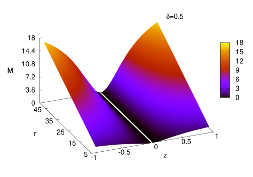
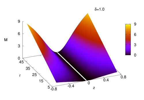
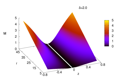
Figure 1: Mass parameters in terms of redshift ($z>0$) or blueshift ($z<0$) of photons emitted by particles in circular orbits of radius $r$ around Chatterjee space-time. The upper graph corresponds to the cases of Kaluza-Klein soliton ($\delta=1/2$), the middle graph corresponds to Schwarzschild black hole ($\delta=1$) and lower graph corresponds to a black hole in the dilaton gravity framework ($\delta=2$). $M$ and $r$ are in geometrized units and scaled by $pM_{\odot}$ where $p$ is an arbitrary proportionality factor.

In regard to the frequency shifts bounds, for $\delta>1/2$, for each $\delta$ there is a $z_{b}$ such that for $|z|<z_{b}$, there exists a unique value of the mass parameter $M(r_{c},z)$, and $z_{b}(\delta)$ does not depend on the radii $r_{c}$ of the circular orbits of photon emitters. $z_{b}=z_{b}(\delta)$ is shown in the upper plot of figure 2, asterisks (in blue) represent the three known cases: Kaluza-Klein solution ($\delta=1/2$), Schwarzschild black hole ($\delta=1$) and dilaton black hole ($\delta=2$). For $\delta$’s in a small vicinity of unity, the bound $z_{b}$ varies little around $1/\sqrt{2}$ which is the Schwarzschild frecuency shift bound. For $\delta\in(1$.$7,3)$, $|z_{b}-1/\sqrt{2}|<0$.$04$. Nonetheless, for $\delta\in(1/\sqrt{5},1/2)$, there is a significant departure from that Schwarzschild bound; furthermore, there are two frequency shifts regions where there is a positive root $M(r_{c},z)$ of (30) corresponding to circular and stable orbits of photon emitters. The lower plot in figure 2 shows these two regions: $|z|>z_{b2}$ and $|z|<z_{b1}$ are physically aceptable. For $0<\delta<1/\sqrt{5}$ the stability condition $V^{\prime\prime}>0$ always holds and there is no bound for $z$.

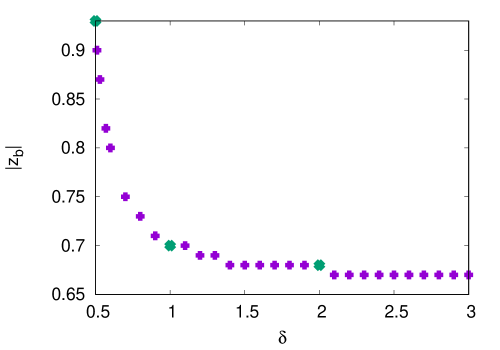
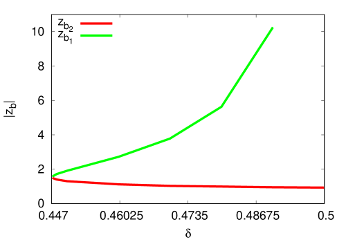
Figure 2: The upper plot shows the value $z_{b}=z_{b}(\delta)$ such that, for $|z|<z_{b}$ there exists a unique value of the mass parameter $M(r,z)$. Asterisks (in blue) represent the three known cases: Kaluza-Klein solution ($\delta=1/2$), Schwarzschild black hole ($\delta=1$) and dilaton black hole ($\delta=2$). In the lower plot, the two regions $|z|>z_{b2}$ and $|z|<z_{b1}$ are physically aceptable.

The upper plot in figuer 3 shows the frequency shift $|z|$ as function of $r/M$ for $\delta=0$.$45$. There is a discontinuity in the frequency shift values physically acceptable corresponding to $|z|>z_{b2}$ (green curve) and $|z|<z_{b1}$ (red curve). The lower plot shows $|z|=|z|(r/M)$ for $\delta=0$.$5$ (red curve) and $\delta=2$ (green curve). In the upper and lower plots, the dashed black curves correspond to the Schwarszchild black hole. For $\delta$’s not close to unity, there is a evident departure from the Schwarzschild curve that might allow us to distinguish (if observational data were available) whether a Schwarzschild or Chaterjee space time is in the center of a galaxy.

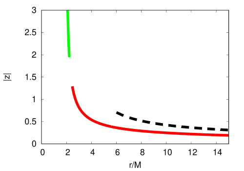
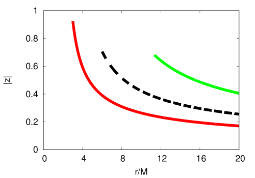
Figure 3: The upper plot ($\delta=0$.$45$) has a gap corresponding to $|z|>z_{b2}$ (green curve) and $|z|<z_{b1}$ (red curve). The lower plot shows $|z|=|z|(r/M)$ for $\delta=0$.$5$ (red curve) and $\delta=2$ (green curve). In both plots, the dashed black curves correspond to the Schwarszchild black hole.

III.2 Gibbons-Maeda space-time

The Gibbons-Maeda metric could represent a charged static black hole with a scalar field GM . This metric reads

$$ds^{2}=-(1-\frac{2M}{r})dt^{2}+(1-\frac{2M}{r})^{-1}dr^{2}+r(r-\frac{Q^{2}}{M})d\Omega^{2}$$ (34)

For $Q=0$ (34) becomes the Schwarzschild black hole. We shall work in the region $r>2M$. Particles will follow circular and equatorial orbits in Gibbons-Maeda space-time provided that

$$L^{2} = \frac{2r(Q^{2}-Mr)^{2}}{2M(2Q^{2}+r^{2})-(6M^{2}+Q^{2})r}>0$$

$$E^{2} = \frac{(r-2M)^{2}(-Q^{2}+2Mr)}{2M(2Q^{2}+r^{2})-(6M^{2}+Q^{2})r}>0.$$ (35)

$L^{2}>0$ holds if and only if

$$P(r,M) = 2M(2Q^{2}+r^{2})-(6M^{2}+Q^{2})r$$ (36)

$$= 2M(r-r_{-})(r-r_{+})>0$$

where

$$r_{\pm}=\frac{6M^{2}+Q^{2}\pm 6\sqrt{(M^{2}-Q^{2}/2)(M^{2}-Q^{2}/18)}}{4M}$$ (37)

In order for $r_{\pm}$ to be real, $2M^{2}>Q^{2}$ must be required. Since for Schwarzschild black hole, circular orbits exist solely for $r>3M$ and $r_{-}\to 0$ and $r_{+}\to 3M$ as $Q\to 0$, we work in the region $r>r_{+}$. It turns out that $r>r_{+}$ and $2M^{2}>Q^{2}$ imply the fullfilment of $E^{2}>0$. Circular orbits are stable as long as the condition

$$V^{\prime\prime}=\frac{-4M^{2}(2Q^{4}-6MrQ^{2}+M(6M-r)r^{2})}{P(r,M)r^{2}(Mr-Q^{2})(r-2M)}>0,$$ (38)

holds and this is so as long as $Mr^{3}-6M^{2}r^{2}+6MQ^{2}r-2Q^{4}>0$. The relation that connects $M,r,Q^{2}$ and $z$ comes from (21) and it reads

$$z^{2}=\frac{2Mr(Mr-Q^{2})}{(r-2M)\left[2M(2Q^{2}+r^{2})-(6M^{2}+Q^{2})r\right]}$$ (39)

In order to find $M=M(r_{c},z;Q^{2})$ one has to solve this cubic equation for $M$. Equation (39) have either three real roots or one real plus two imaginary roots. We keep only the real positive roots $M=M(r_{c},z;Q^{2})$ that fulfill the conditions for circular and stable orbits and it turns out that, from the analytic Cardan’s formula, the only one that satisfies those conditions is

$$M(r_{c},z,Q^{2})=\left[2\sqrt{\frac{-p}{3}}\cos{(\frac{\phi}{3}+\frac{4\pi}{3})}-\frac{a}{3}\right]\quad\mbox{where}$$

$$p = b-\frac{a^{2}}{3},\quad q=c-\frac{ab}{3}+\frac{2a^{3}}{27},\quad\phi=\cos^{-1}\left[\frac{\sqrt{27}q}{2p\sqrt{-p}}\right]$$

$$a = -\left(\frac{2Q^{2}}{3r_{c}}+\frac{5z^{2}+1}{6z^{2}}r_{c}\right),\quad c=-\frac{r_{c}Q^{2}}{12}$$

$$b = \left(Q^{2}\frac{3z^{2}+1}{6z^{2}}+\frac{r_{c}^{2}}{6}\right).$$ (40)

This analysis is performed numerically in the following manner: we set a domain $\mathcal{D}=(Q_{1},Q_{2})\times(r_{1},r_{2})\times(z1,z2)$, for each $q\in\mathcal{D}$ the roots of (39) are found. With these roots at hand, we check whether the following conditions are all satisfied: (i) $r>2M$, (ii) $r>r_{+}$, (iii) $2M^{2}>Q^{2}$ and (iv) $Mr^{3}-rM^{2}r^{2}+6MQ^{2}r-2Q^{4}>0$. The second and third inequalities guarantee that indeed, we have circular and equatorial orbits; the fourth inequality guarantees stability of these orbits. As mentioned, it turns out that the only root satisfying all the conditions has the form given by (40). For given values of $r_{c}$ and $Q^{2}$, we search for the minimum and maximum value of $z$ for which these four conditions simultaneously hold, this process yields bounds of the frequency shifts. For $Q=0$, the result for Schwarzschild ($|z|<z_{b}=1/\sqrt{2}$) is recovered as it should be. Figure 4 shows the surfaces $z_{min}=z_{min}(r_{c},Q^{2})$ and $z_{max}=z_{max}(r_{c},Q^{2})$. Only for frequency shifts $z$ such that $|z|\in(z_{min},z_{max})$, the corresponding values for the mass parameter $M=M(r_{c},z,Q)$ are acceptable. We observe that the larger $Q^{2}$ is, the narrower the gap between $z_{min}$ and $z_{max}$ becomes. For large $Q^{2}$’s and small $r_{c}$’s, $z_{min}$ and $z_{max}$ sharply increase.

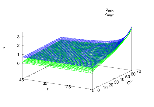
Figure 4: The two redshift surfaces $z_{min}$ and $z_{max}$ as function of the radius $r$ of circular orbits followed by photon emitters around a Gibbson-Maeda spacetime and its charge parameter $Q^{2}$ are shown. Only for redshifts $z\in(z_{min},z_{max})$ the corresponding values $M=M(r,z,Q^{2})$ are acceptable. $M$, $Q$, and $r$ are in geometrized units and scaled by $pM_{\odot}$ where $p$ is an arbitrary factor of proportionality .

Due to the condition (iii) $2M^{2}>Q^{2}$, as the charge $Q^{2}$ increases, the corresponding acceptable value $M(r_{c},z,Q^{2})$ also increases. The upper plot of figure 5, shows $M=M(r_{c},z,Q^{2}=10)$ and $M>\sqrt{5}$ as it should be according condition (iii), the lower plot shows $M=M(r_{c},z,Q^{2}=70)$ and $M>\sqrt{35}$. $M$, $r_{c}$ and $Q$ are in geometrized units and scaled by $pM_{\odot}$ where $p$ is an arbitrary proportionality factor. For $Q=0$, the result of the Schwarzschild black hole shown in the middle plot of figure 1 with $z_{b}=1/\sqrt{2}$ is recovered.

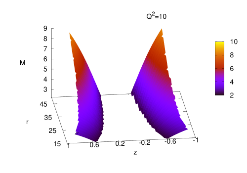
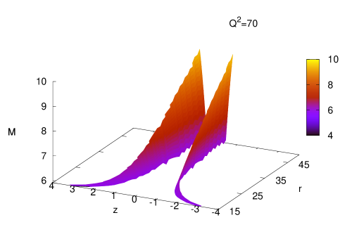
Figure 5: Mass parameters in terms of redshift ($z>0$) and blueshift ($z<0$) of photons emitted by particles in circular orbits of radius $r$ around Gibbons-Maeda space-time. The upper plot shows $M(r,z,Q^{2}=10)$ and the lower plot $M(r,z,Q^{2}=70)$. $M$, $r$ and $Q$ are in geometrized units and scaled by $pM_{\odot}$ where $p$ is an arbitrary proportionality factor.

IV Final remarks

There have been efforts to find astrophysical signatures of scalar fields. In Matos-Brena the following spacetime was considered

$$ds^{2} = -(1-\frac{2M}{r})dt^{2}+e^{2k_{s}}\frac{dr^{2}}{1-2M/r}$$ (41)

$$+r^{2}\left(e^{2k_{s}}d\theta^{2}+\sin{\theta}d\phi^{2}\right)$$

where

$$e^{2k_{s}} = \left(1+\frac{M^{2}\sin^{2}{\theta}}{r^{2}(1-2M/r)}\right)^{-1/b^{2}}$$

$$\Phi = \frac{1}{2b}\ln\left(1-\frac{2M}{r}\right),$$ (42)

with $b$ an integration constant. As $b\to\infty$, the scalar field vanishes and the Schwarzschild black hole is recovered. The metric (41) was employed to model the Sun and the deflection of light rays passing nearby was computed, the authors found that the current observational errors for this effect set the limit $b>0.02$. One of their conclusions was that even if a scalar field of the form (42) were actually present in the solar system, it cannot be presently detected. If we apply HN formalism to the metric (41) considering equatorial and circular orbits, then $M=M(r_{c},z)$ and the bound for $z$ would be exactly the same as the one for the Schwarzschild black hole since the components $g_{rr}$ and $g_{\phi\phi}$ are just the same. As a matter of fact, any solution to the EMD theory that for equatorial and circular orbits leaves $g_{rr}=(1-2M/r)^{-1}$ and $g_{\phi\phi}=r^{2}$ would yield the same results as for that of the Schwarzschild metric.

From our analysis on the Chatterjee spacetime, we observed that, for $\delta$’s not close to unity, the departure of our results from those of the Schwarzschild black hole is noticeable and becomes truely apparent for $\delta\in(1/\sqrt{5},1/2)$ where there are two frequency shifts regions where there is a positive root $M(r_{c},z)$ of (30) corresponding to circular and stable orbits of photon emitters. For the Gibbons-Maeda metric, the bounds of frequency shifts are two surfaces $z_{min}(r_{c},Q^{2})$ and $z_{max}(r_{c},Q^{2})$ whose gap narrows as $Q^{2}$ increases and $r_{c}$ decreases their values, as shown in figure 4. It would be interesting to apply this formalism to rotating dilaton black holes horne and contrast the results with those found in us for the Kerr black hole.

ACKNOWLEDGMENTS

S.V-A acknowledges partial support from PRODEP, under 4025/2016RED project. F.A and R. B. acknowledge partial support by CIC-UMSNH. The authors thank professor Ulises Nucamendi for useful comments and discussions on the results of this work.

References

- (1) M. B. Begelman, Evidence for black holes, Science 300, 1898 (2003). Z. Q. Shen, K. Y. Lo, M.-C. Liang, P. T. P. Ho, and J.-H. Zhao, A size of 1 au for the radio source Sgr at the center of the Milky Way, Nature (London) 438, 62 (2005). A. M. Ghez, S. Salim, N. N. Weinberg, J. R. Lu, T. Do, J. K. Dunn, K. Matthews, M. R. Morris, S. Yelda, E. E. Becklin, T. Kremenek, M. Milosavljevic, and J. Naiman, Measuring distance and propereties of the Milky Way’s central supermassive black hole with stellar orbits, Astrophys. J. 689, 1044 (2008). M. R. Morris, L. Meyer, and A. M. Ghez, Galactic center research: Manifestations of the central black hole, Res. Astron. Astrophys. 12, 995 (2012)
- (2) Alfredo Herrera and Ulises Nucamendi, Kerr black hole parameters in terms of the redshift/blueshift of photons emitted by geodesic particles, Phys. Rev. D 92, 045024 (2015).
- (3) Ricardo Becerril, Susana Valdez-Alvarado, Ulises Nucamendi, Obtaining mass parameters of compact objects from redshifts and blueshifts emitted by geodesic particles around them, Phys. Rev. D 94, 124024 (2016).
- (4) B. Aschenbach, N. Grosso, D. Porquet and P. Predehl, X-ray flares reveal mass and angular momentum of the Galactic Center black hole, A & A 417, 71–794, 8 (2004).
- (5) T. Matos, F.S. Guzman and L. Ureña. Scalar Fields as Dark Matter in the Universe, Class. Quantum Grav. 17, (2000) 1707. Mikel Susperregi, Dark matter and dark energy from an inhomogeneous dilaton, Phys. Rev. D 68, 123509 (2003).
- (6) T. Matos and F.S. Guzman. Scalar fields as dark matter in spiral galaxies, Class. Quantum Grav. 17, L9 (2000).
- (7) T. Matos and R. Becerril, An axially symmetric scalar field as a gravitational lens, Class. Quantum Grav. 18, 2015 (2001).
- (8) Eric W. Hirschmann, Luis Lehner, Steven L. Liebling, and Carlos Palenzuela, Black Hole Dynamics in Einstein-Maxwell-Dilaton Theory. arXiv:1706.09875, (2017).
- (9) T. Matos and A. Macías. Black holes from generalized Chatterjee solutions in dilaton gravity, Modern Physics Letters A 9, 3707 (1994).
- (10) G.W.Gibbons and Kei-ichi Maeda. Black holes and membranes in higher-dimensional theories with dilaton fields, Nuclear Physics B 298, 741 (1988). David Garfinkle, Gary T. Horowitz and Andrew Strominger, Charged black holes in string theory, Phys. Rev. D 43, 3140 (1991).
- (11) William H. Press, Saul A. Teukolsky, William T. Vetterling and Brian P. Flannery, Numerical Recipes. Cambridge University Press.
- (12) T. Matos and Hugo V. Brena, Possible astrophysical signatures of scalar fields, Class. Quantum Grav. 17, 1455 (2000).
- (13) James H. Horne and Gary T. Horowitz, Rotating dilaton black holes. Phys. Rev. D 46, 1340 (1992).