Topology of Privacy:
Lattice Structures and Information Bubbles
for Inference and Obfuscation

Abstract

Information has intrinsic geometric and topological structure, arising from relative relationships beyond absolute values or types. For instance, the fact that two people did or did not share a meal describes a relationship independent of the meal’s ingredients. Multiple such relationships give rise to relations and their lattices. Lattices have topology. That topology informs the ways in which information may be observed, hidden, inferred, and dissembled. Privacy preservation may be understood as finding isotropic topologies, in which relations appear homogeneous. Moreover, the underlying lattice structure of those topologies has a temporal aspect, which reveals how isotropy may contract over time, thereby puncturing privacy.

Dowker’s Theorem establishes a homotopy equivalence between two simplicial complexes derived from a relation. From a privacy perspective, one complex describes individuals with common attributes, the other describes attributes shared by individuals. The homotopy equivalence is an alignment of certain common cores of those complexes, effectively interpreting sets of individuals as sets of attributes, and vice-versa. That common core has a lattice structure. An element in the lattice consists of two components, one being a set of individuals, the other being an equivalent set of attributes. The lattice operations join and meet each amount to set intersection in one component and set union followed by a potentially privacy-puncturing inference in the other component.

One objective of this research has been to understand the topology of the Dowker complexes, from a privacy perspective. First, privacy loss appears as simplicial collapse of free faces. Such collapse is local, but the property of fully preserving both attribute and association privacy requires a global condition: a particular kind of spherical hole. Second, by looking at the link of an identifiable individual in its encompassing Dowker complex, one can characterize that individual’s attribute privacy via another sphere condition. This characterization generalizes to certain groups’ attribute privacy. Third, even when long-term attribute privacy is impossible, homology provides lower bounds on how an individual may defer identification, when that individual has control over how to reveal attributes. Intuitively, the idea is to first reveal information that could otherwise be inferred. This last result highlights privacy as a dynamic process. Privacy loss may be cast as gradient flow. Harmonic flow for privacy preservation may be fertile ground for future research.

1 Introduction

Privacy is the ability of an individual or entity to control how much that individual or entity reveals about itself to others. Fundamental research into privacy seeks to understand the limits of that ability.

A brief history of privacy should include the following:

• The right to privacy as a legal principle, appearing in an 1890 Harvard Law Review article [24]. The article was a reaction to the then modern technology of photography and the dissemination of gossip via print media.

• A demonstration linking supposedly anonymous public information with other more specific public data, thereby revealing sensitive attributes [21]. The demonstration employed zip code, gender, and birth date to link anonymous public insurance summaries with voter registration data. Doing so produced the health record of the governor of Massachusetts. This privacy failure suggested a first form of homogenization, called $k$-anonymity. Roughly, the idea was to structure databases in such a way that a database could respond to any query with an answer consisting of no fewer than $k$ individuals matching the query parameters.

• The discovery that it is impossible to preserve the privacy of an individual for even a single attribute in the face of repeated statistical queries over a population [2], unless  answers to those queries are purposefully perturbed with noise of magnitude on the order of at least $\sqrt{n}$. Here $n$ is the size of the population. The significance of this discovery is to underscore how difficult it is to preserve privacy while retaining information utility.

• Netflix Prize. In 2006, Netflix offered a $1M prize for an algorithm that would predict viewer preferences better than Netflix’s internal algorithm. Netflix made available some of its historical user preferences, in anonymized form, as a basis for the competition. Once again, it turned out that one could link this anonymized data with other publicly available databases, resulting in the potential (and in some cases actual) identification of Netflix viewers, thereby de-anonymizing their viewing history [17]. Whereas in the earlier health example, a few specific observables made linking possible (global coordinates, one might say, namely zip code, gender, birth date), in the Netflix example, the intrinsic geometric structure of the database facilitated linking via a wide variety of observables (local landmarks, one might say, namely movies that were characteristic for each individual). Key was sparsity of information: 8 movie ratings and dates were generally enough to uniquely characterize $99\%$ of viewers in the Netflix Prize dataset, even with errors in the ratings and dates.

• Differential Privacy [5, 4] seeks to avoid the previous privacy failures by focusing on local rather than absolute privacy guarantees. The underlying approach in differential privacy is for a database to answer statistical queries with a particular stochastic blurring. Specifically, the probability that an interrogator of the database will make any particular inference should depend only in a very small way on whether any one individual does or does not have a particular attribute (such as even being in the database). We might call this stochastic homogeneity.

• Randomized Response. Differential privacy is further significant because it makes explicit the dynamic nature of privacy; there may be no enduring privacy guarantees but there are differential guarantees. A particular form is randomized response, a technique used in the social sciences to elicit reliable aggregate answers to sensitive questions, asking the question of many people, but perturbing individual answers stochastically so as not to learn much about any one individual from any single response [23]. A version has been employed by Google to find malware [8].

Privacy has both a combinatorial component and a statistical component. Prior research has largely focused on statistical techniques, both to preserve privacy and to puncture privacy. One of the goals of this research is to understand the combinatorial component of privacy, leading naturally to methods from combinatorial topology.

A desire to understand the geometry and topology of the types of inferences revealed by the Netflix Prize formed the specific motivation for our research initially. Subsequently, we realized that the lattice structure found in that geometry had broader applicability, providing an ability to model the dynamics of privacy more generally.

2 Outline

The remaining sections and appendices present the following material:

Main Narrative:

3:

Toy examples illustrating how a relation may lead to privacy loss in the presence of background information. The section introduces the doubly-labeled poset  associated with a relation, to model such inferences. The elements of the poset are ordered pairs, each a set of individuals and a set of attributes.

This section also states and discusses assumptions that hold throughout the report.

4:

Formal description of the Galois connection associated with a relation. The section first defines, for any relation, two simplicial complexes called Dowker complexes. One complex represents sets of individuals with shared attributes, the other represents sets of attributes shared by individuals. The Galois connection then establishes a homotopy equivalence between the Dowker complexes, thereby generating the relation’s doubly-labeled poset. The homotopy equivalence gives rise to closure operators, with “closure” in the poset modeling inference of unobserved attributes from observed attributes (or unobserved individuals from observed individuals).

This section also defines attribute privacy  and association privacy.

5:

A characterization of privacy in terms of the absence of free faces in the relevant Dowker complex. This section observes as well that the only connected relations able to preserve both attribute and association privacy must look either like linear cycles or like boundary complexes. In particular, the number of individuals and attributes must be the same.

6:

Conditional relations, as models for simplicial links. A conditional relation is much like a conditional probability distribution. It might, for instance, represent the possible arrangement of remaining attributes among individuals, after some attributes have already been observed.

7:

A characterization of individual and group attribute privacy in terms of spherical and boundary complexes for the relation that models the individual’s or group’s link in its Dowker complex.

8:

A brief exploration of holes in relations, focusing on attribute spaces generated by bits.

9:

A small example exploring the possibility of increasing privacy by change-of-coordinate transformations.

10:

A lengthy exploration of how someone can delay identification, by releasing attributes selectively in a particular order. This idea leads to the notion of informative attribute release sequences, how to find such sequences in the Galois lattice, and the use of homology as a lower bound for the number and length of such sequences.

11:

Computation of the homology and maximal informative attribute release sequences present in two relations found on the world wide web. One relation describes Olympic athletes and their medals, the other describes jazz musicians and their bands.

12:

A more general perspective of inference as motion in lattices, not necessarily directly derived from a relation. This perspective suggests connections to randomized response techniques.

13:

An examination of the ability to obfuscate strategies and/or goals in graphs where motions may be nondeterministic or stochastic.

14:

A possible category for representing relations, along with an analysis of morphism properties. The morphisms between relations in this category induce simplicial and therefore continuous maps between the relations’ corresponding Dowker complexes.

This section further shows by example how a morphism of relations, when it is surjective at the set level, generates the full lattice of the codomain’s relation, via closure under lattice operations.  (A general proof appears in Appendix I.)

15:

Some thoughts for the future, including an example that connects stochastic sensing to the Galois lattice.

Appendices:

A:

A summary of the basic notation and definitions used in this report.

B:

A summary of the basic tools used in this report, establishing the homotopy equivalences and closure operators mentioned previously.

C:

Construction of links and deletions, and examination of the privacy properties each inherits from its encompassing relation. This appendix explores the significance of free faces in the Dowker complexes. The appendix further proves that a relation with more attributes than individuals cannot preserve attribute privacy for every individual.

D:

Proof that the problem of finding a minimal set of attributes from which another attribute may be inferred is $N\!P$-complete. This stands in contrast to the observation that the problem of finding some  set of attributes from which another may be inferred (or reporting that no such set exists) is computable in polynomial time.

E:

Detailed proofs of the results claimed in Section 7. Also a detailed proof of the assertion from Section 5 regarding relations that preserve both attribute and association privacy.

F:

Detailed proofs of the connection between maximal chains in a relation’s Galois lattice and informative attribute release sequences. When such sequences are order-independent they correspond to spherical holes, leading to the concept of an isotropic  sequence.

G:

Detailed proof that homology establishes a lower bound for the number and length of maximal chains in a relation’s Galois lattice, and thus for the number and length of informative attribute release sequences that may be used to delay identification.

H:

An application of the previous results with the aim of obfuscating the identification of strategies for attaining goals in graphs with uncertain transitions.

I:

Detailed proofs of the assertions of Section 14 regarding morphisms.

J:

Some additional examples:

1. Dunce Hat: modeled as a relation for which the Dowker attribute complex is contractible but has no free attribute faces, meaning the relation preserves attribute privacy.

2. Disinformation: An example that glues together two copies of the Möbius strip, thereby removing free faces and creating a form of homogeneity that preserves attribute privacy yet retains the utility of identifiability.

3. Insufficient Representation: If there are insufficiently many individuals in a relation generated by bits, attribute inference is possible.

4. A Matching Example: When many individuals are being observed, cardinality constraints allow for inferences beyond those discussed in this report.

List of Primary Symbols

Symbol	Typical Meaning	Page(s)
$X$	discrete space of individuals	1, • ‣ A.4
$Y$	discrete space of attributes	1, • ‣ A.4
$R$	relation on ${X}\mskip-1.8mu\times{Y}$	1, • ‣ A.4
$X_{y}$	individuals with attribute $y$ (usually in the context of relation $R$)	1, • ‣ A.4
$Y_{x}$	attributes of individual $x$ (usually in the context of relation $R$)	1, • ‣ A.4
$Q$	another relation, often representing a link in a simplicial complex	7, 55, 19
$\Sigma,\Gamma$	generic simplicial complexes  (sometimes merely sets)	• ‣ A.1
$\Psi_{R}$	complex; simplices are sets of individuals with a common attribute	1, • ‣ A.4
$\Phi_{R}$	complex; simplices are sets of attributes shared by some individual	1, • ‣ A.4
$\sigma$	usually a simplex representing individuals in $\Psi_{R}$
$\gamma$	usually a simplex representing attributes in $\Phi_{R}$
$\phi_{R}$	homotopy equivalence from sets of individuals to shared attributes	2, • ‣ A.4
$\psi_{R}$	homotopy equivalence from sets of attributes to sharing individuals	2, • ‣ A.4
$P$	partially ordered set (poset)	• ‣ A.2
${\mathfrak{F}}(\Sigma)$	face poset of the simplicial complex $\Sigma$	2, • ‣ A.2
$\Delta(P)$	order complex of the poset $P$	4.2, • ‣ A.2
$P_{R}$	doubly-labeled poset associated with relation $R$	3.3, 3, • ‣ A.4
$L$	(inference) lattice	(29) • ‣ A.3
$P^{+}_{R}$	Galois lattice formed from $P_{R}$	13, • ‣ A.4
$\{(\sigma_{k},\gamma_{k})<\cdots<(\sigma_{0},\gamma_{0})\}$	chain of length $k$ in the lattice $P^{+}_{R}$	21, F, • ‣ A.2
$y_{1},\ldots,y_{k}$	informative attribute release sequence (iars) of length $k$ (for relation $R$)	14
$V$	set of vertices in a simplicial complex or states in a graph
${\partial{(V)}}$	simplicial boundary complex with vertices $V$	5.3, 1
$\mathbb{S}^{\kern 0.56001pt{-1}}$	sphere of dimension $-1$, modeling the empty complex $\{\emptyset\}$	• ‣ A.1
$\mathbb{S}^{1}$	circle	5.3
$\mathbb{S}^{\kern 0.56001pt{n-2}}$	sphere of dimension $n\!-\!2$	5.3, 1
$C_{k}(\Sigma;\mathbb{Z})$	group of simplicial $k$-chains over $\Sigma$, with integer coefficients	• ‣ A.1
$\widetilde{\partial}$	(family of) reduced boundary map(s)  $C_{k}(\Sigma;\mathbb{Z})\rightarrow C_{k-1}(\Sigma;\mathbb{Z})$	2
$\widetilde{H}_{k}(\Sigma;\mathbb{Z})$	reduced $k$-dimensional homology group of $\Sigma$, with integer coefficients	• ‣ A.1
$G$	a graph, generally with nondeterministic and/or stochastic actions	13.1, • ‣ 13.2
$\Delta_{G}$	strategy complex of a graph	45, • ‣ 13.2
${\overline{\Delta}_{G}}$	source complex of a graph	H.1
$\simeq$	homotopy equivalence	• ‣ A.1
$*$	simplicial join	• ‣ A.1
$\vee$	either topological wedge sum or lattice join	• ‣ A.1, A.3
$\wedge$	lattice meet	A.3

3 Privacy: Relations and Partially Ordered Sets

Our investigation of privacy in this report will be in terms of relations. As we will see in this section and the next, relations give rise to simplicial complexes, which give rise to partially ordered sets, which expose an underlying lattice structure. That lattice structure makes explicit how privacy may be preserved or lost through so-called background knowledge. As we will see in Section 10, the lattice structure also makes explicit how identification may be delayed by careful release of information.

3.1 A Toy Example: Health Data and Attribute Privacy

Consider the following relation $H$, describing the results of a hypothetical health study for four patients and three attributes. The patients have been anonymized and are represented simply by the set of numbers $\{1,2,3,4\}$. The three attributes are drawn from the set $\{\hbox{\sc smokes},\hbox{\sc has\_cancer},\hbox{\sc drinks\_soda}\}$.

One can describe a relation equivalently either as a matrix or as a set of ordered pairs:

Relation $H$ as a matrix:

$$\qquad\qquad\qquad\begin{array}[]{c|ccc}H&\hbox{\sc smokes}&\hbox{\sc has\_cancer}&\hbox{\sc drinks\_soda}\\[2.0pt] \hline\cr 1&\bullet&\bullet&\\ 2&&\bullet&\bullet\\ 3&&&\bullet\\ 4&&&\bullet\\ \end{array}$$

Relation $H$ as a set of ordered pairs:

$$\big{\{}(1,\hbox{\sc smokes}),\,(1,\hbox{\sc has\_cancer}),\,(2,\hbox{\sc has\_cancer}),\,(2,\hbox{\sc drinks\_soda}),\,$$

$$(3,\hbox{\sc drinks\_soda}),\,(4,\hbox{\sc drinks\_soda})\big{\}}.$$

Assumptions

Before discussing privacy further, we make some assumptions that hold throughout the report:

Assumption of Relational Completeness:

We assume that any given relation is not missing any observable elements, relative to some external (unspecified) ground truth.

For example, if we observe that someone drinks soda and has cancer in relation $H$, then we would conclude that we are observing individual #2. We would be surprised to see that individual smoke. If for some reason we ever do see the individual smoke, then we would deem our observations to be  inconsistent  with relation $H$. — The meaning of inconsistency depends on context. At top-level, an inconsistency may mean that the relation or observation is errorful. When making conditional observations, an inconsistency may actually supply useful information, as we will see in Lemma 12 on page 12.

Comment: A relation may contain extra elements, as may be useful for disinformation. A relation could even be missing elements that represent valid ordered pairs, so long as those elements are deemed to be unobservable for that relation. For example, one may have a time series of relations in which some attributes only become observable at later times. In such a setting, one may never know whether a particular individual had a particular attribute at an earlier time.

In the example, it could be that individual #1 drinks soda, but that it is impossible to observe this fact. In that case, relation $H$ would still satisfy the assumption of relational completeness, even though $H$ contains no entry indicating that individual #1 drinks soda.

Assumption of Observational Monotonicity:

Even though we assume relations are complete, we do not  assume that observations are complete. Instead, we assume: The observation of a particular attribute for an individual is meaningful; lack of such an observation does not necessarily imply that the individual fails to have the unobserved attribute. The motivation for this assumption is that one may yet discover that the individual has the attribute. For example, suppose we observe someone (whom we know to be part of relation $H$) drinking soda. Even if that is all we observe, we do not  conclude that the individual is cancer free. It could be that we might yet observe the individual to have cancer.

If absence of an attribute is significant and  that absence is observable, then both the attribute and its negation could and perhaps should appear explicitly in the relation as distinct mutually exclusive attributes. For instance, Prime versus Composite might be such a pair of attributes for integers greater than 1.

Assumption of Observational Accuracy:

We assume that observations are accurate. For instance, if we observe an integer to be either Prime or Composite, then we do so correctly.

Comments:

The three assumptions above are desiderata for how the mathematical abstractions of this report fit into the real world.  Some comments are in order:

• In and of itself, a relation defines a particular kind of world, a bipartite graph, and there is no external ground truth.

• In such a world, the completeness, monotonicity, and accuracy assumptions describe a sensor and the meaning of observations made by the sensor.

The purpose of the assumptions in the real world is largely to ensure consistency between different relations and with possible observations.

• The monotonicity assumption is important because information generally aggregates asynchronously. Together with the other assumptions, this assumption means that one may view relations as monotone Boolean functions, and thus may leverage methods from combinatorial topology.

• One may incorporate some errors into the relational and observational models, for instance by blurring a relation. For very large integers, a relation might allow some integers to have both  Prime and Composite as attributes. Although an integer is one or the other, the relation admits to uncertainty by allowing both attributes at once. Indeed, some relations purposefully introduce such blurring to preserve privacy, as with randomized response [23]. In robotics, natural relational blurring arising from noisy but environment-compatible sensors can actually help establish the topology of a region, for instance by dualizing sensors and landmarks [11].

Privacy Implications

Making the health study $H$ of page 3.1 publicly available has some privacy implications, including the following:

• Suppose someone named Bob tells his friend Alice that he was part of the study. Alice knows that Bob smokes everywhere he goes, so she can infer that he is Patient #1 and has cancer.  (This is an example of inference in a relation using background knowledge.)

• Suppose Cindy is Patient #2. She has full attribute privacy as far as relation $H$ is concerned. In particular, as we saw already, Cindy can tell her friends that she was part of the health study while drinking soda and those friends will not be able to conclude that she has cancer.

• Patients #3 and #4 are not only indistinguishable from each other but also from Cindy (patient #2), as far as relation $H$ is concerned. This is a very strong form of anonymity. Even if one of them reveals that s/he drinks soda, s/he will remain indistinguishable from the other two patients who drink soda.

Caveat: In the last case, if Cindy reveals that she has cancer and is seen to be different from the other individuals, then one may be able to remove her from the relation, narrowing the focus and creating a new relation that may allow additional inferences. Similar caveats hold for the other bullets. Deletions are discussed further in Appendix C.

Modifying a Relation to Increase Privacy

We can make a small change in relation $H$ that enhances privacy. If we artificially give patient #3 the attribute smokes, then we obtain the following modified relation $H^{\prime}$:

$$\begin{array}[]{c|ccc}H^{\prime}&\hbox{\sc smokes}&\hbox{\sc has\_cancer}&\hbox{\sc drinks\_soda}\\[2.0pt] \hline\cr 1&\bullet&\bullet&\\ 2&&\bullet&\bullet\\ 3&\bullet&&\bullet\\ 4&&&\bullet\\ \end{array}$$

Now Bob may reveal to Alice that he was part of the health study without Alice being able to infer that he has cancer, even though she knows that everyone knows that he smokes. In fact, more generally, one can no longer infer cancer from smoking, within the relation.

Such an artificial entry in the relation is a form of disinformation. It certainly skews statistics and utility. It also increases privacy.

3.2 A Dual Perspective: Payroll Data and Association Privacy

The previous example examined a relation from the perspective of attribute privacy: we were interested in understanding how observation of some attribute(s) implied other attribute(s), possibly identifying an individual. A dual perspective is association privacy, in which one seeks to understand how some associations between individuals imply others.

The following hypothetical “salary” relation $S$ has the same matrix structure as relation $H$ did earlier, but with different semantics. This relation represents employees $\{\hbox{Bob},\hbox{Mary},\hbox{Frank},\hbox{Julie}\}$ working on secret projects $\{{\tt a},{\tt b},{\tt c}\}$. Now the employee names are visible so that a payroll clerk can disburse salaries correctly, but the actual projects are anonymous.

$$\begin{array}[]{c|ccc}S&{\tt a}&{\tt b}&{\tt c}\\[2.0pt] \hline\cr\hbox{Bob}&\bullet&\bullet&\\ \hbox{Mary}&&\bullet&\bullet\\ \hbox{Frank}&&&\bullet\\ \hbox{Julie}&&&\bullet\\ \end{array}$$

The salary relation $S$ has some implications for association privacy, including the following:

• If someone tells the payroll clerk that Julie is the lead of a very important project with valuable information, then the payroll clerk can infer that Mary and Frank have also been exposed to valuable information.

• In contrast, if someone tells the payroll clerk that Bob is running a very important project, then the payroll clerk does not have enough information to conclude that Mary is also working on an important project.

Regarding disinformation: Observe how adding the artificial entry $(\hbox{Julie},{\tt a})$ prevents the payroll clerk from using the relation to infer that Mary and Frank have valuable information, even if the payroll clerk learns via background information that Julie is the lead of a very important project with such information:

$$\begin{array}[]{c|ccc}S^{\prime}&{\tt a}&{\tt b}&{\tt c}\\[2.0pt] \hline\cr\hbox{Bob}&\bullet&\bullet&\\ \hbox{Mary}&&\bullet&\bullet\\ \hbox{Frank}&&&\bullet\\ \hbox{Julie}&\bullet&&\bullet\\ \end{array}$$

3.3 Privacy Preservation and Loss: A Poset Model

$\begin{array}[]{c|ccc}R&{\tt a}&{\tt b}&{\tt c}\\[2.0pt] \hline\cr 1&\bullet&\bullet&\\ 2&&\bullet&\bullet\\ 3&&&\bullet\\ 4&&&\bullet\\ \end{array}$

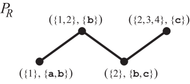
Figure 1: Relation $R$ serves as a model for the two examples of Sections 3.1 and 3.2. The doubly-labeled poset $P_{R}$ describes the inferences facilitated by $R$.

Figure 1 shows a relation $R\mskip 2.0mu$ that serves as a model for both the health example of Section 3.1 and the payroll example of Section 3.2. The relation is identical to those given earlier, but with abstract labels in place of both individuals and attributes. The figure also depicts a partially ordered set (poset) $P_{R}$, designed to model the inferences discussed previously. We refer to that poset as the doubly-labeled poset associated with $R$. We next discuss the semantics of $P_{R}$. Section 4 discusses the construction of $P_{R}$. The underlying concepts are important throughout the report.

Semantics of the poset $P_{R}$:

• Each element in the poset consists of an ordered pair $(\sigma,\gamma)$, with $\emptyset\neq\sigma\subseteq\{1,2,3,4\}$ describing a set of individuals and $\emptyset\neq\gamma\subseteq\{{\tt a},{\tt b},{\tt c}\}$ describing a set of attributes. We say that the poset element is labeled with $\sigma\!$ and $\gamma$. The meaning of such a double-labeling (with respect to the information described by relation $R$) is:

  1. All individuals in $\sigma$ have all attributes in $\gamma$.

  2. If (and only if) an individual has at least all the attributes in $\gamma$, then that individual must be in $\sigma$. For example, we see that individual #2, and only individual #2, has both attributes ${\tt b}$ and ${\tt c}$ in $R$.

  3. If (and only if) an attribute is shared by at least all individuals in $\sigma$, then that attribute must be in $\gamma$. For example, individual #1 has both attributes ${\tt a}$ and ${\tt b}$, so $P_{R}$ cannot contain simply $(\{1\},\{{\tt a}\})$, but must contain $(\{1\},\{{\tt a},{\tt b}\})$.

• The partial order for $P_{R}$ is described by the edges in the figure. There is an edge between two elements $(\sigma_{1},\gamma_{1})$ and $(\sigma_{2},\gamma_{2})$ of $P_{R}$ whenever the corresponding sets are subset comparable. In particular, $(\sigma_{1},\gamma_{1})\leq(\sigma_{2},\gamma_{2})$ in $P_{R}$ precisely when $\sigma_{1}\subseteq\sigma_{2}$ and $\gamma_{1}\supseteq\gamma_{2}$. [Observe that the comparability ($\subseteq$ versus $\supseteq$) is opposite for $\sigma$ versus $\gamma$.]

Using the poset $P_{R}$ for attribute inference:

Suppose $\gamma$ is any  nonempty subset of attributes in $\{{\tt a},{\tt b},{\tt c}\}$. Then one of (i) or (ii) holds:

1. Perhaps no individual modeled by $R\hbox{\hskip 1.0pt}$ has all the attributes $\gamma$. For example, no individual has attributes $\gamma=\{{\tt a},{\tt c}\}$. We would not expect to see $\gamma$ and so $\gamma$ does not appear in the poset $P_{R}$.

2. Alternatively, $\gamma$ is a subset of at least one set of attributes that does appear in the poset. In this case, one may be able to enlarge $\gamma$ nontrivially, resulting in privacy loss.

   For example, imagine we discover that a friend with attribute ${\tt a}$ is modeled by the given relation (e.g., Bob, who smokes, says he is part of the health study $H$).
   Using $\gamma=\{{\tt a}\}$, the poset then allows us to infer that Bob must also have attribute ${\tt b}$ (that is, has_cancer).  Why?  Because $\{{\tt a},{\tt b}\}$ is a minimal set in $P_{R}$ containing $\{{\tt a}\}$.

   We can say yet more: The element labeled with $\{{\tt a},{\tt b}\}$ is also labeled with $\{1\}$. So now we have de-anonymized  individual #1 (identifying him to be Bob).

   Regardless of whether Bob ever actually talks to us, the poset tells us that individual #1 could  suffer privacy loss, and in fact, is uniquely identifiable in the context of relation $R$ without needing to reveal everything about himself.

Similar reasoning is possible for association inference, as we saw earlier.

$\begin{array}[]{c|ccc}R^{\prime}&{\tt a}&{\tt b}&{\tt c}\\[2.0pt] \hline\cr 1&\bullet&\bullet&\\ 2&&\bullet&\bullet\\ 3&\bullet&&\bullet\\ 4&&&\bullet\\ \end{array}$

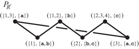
Figure 2: A relation $R^{\prime}$, along with its doubly-labeled poset $P_{R^{\prime}}$. The relation preserves attribute privacy but allows a small amount of association inference: If ones sees individual #4 in some context ${\tt c}$, then one can infer that individuals #2 and #3 are also present in that same context, without needing to observe them directly.

Disinformation Revisited:

Figure 2 shows relation $R^{\prime}$, constructed from $R$ by adding an entry of disinformation, much as we constructed $H^{\prime}$ from $H$ earlier. The figure also shows the corresponding doubly-labeled poset $P_{R^{\prime}}$. Observe that it is no longer possible to infer $\{{\tt a},{\tt b}\}$ from $\{{\tt a}\}$, because $\{{\tt a}\}$ now appears directly in the poset. The added entry $(3,{\tt a})$ in $R^{\prime}$ has increased attribute privacy compared to $R$.

There is, however, still some opportunity for making association inferences. For instance, knowing that individual #4 (Julie, earlier) works on an important secret project still allows the inference that individuals #2 and #3 have valuable information. That is because the minimal set containing $\{4\}$ in the poset is $\{2,3,4\}$. Notice that no such association inference is possible if someone says that individual #3 works on an important secret project, though that would have been possible in the original relation $R$.

Comment:

Artificial entries can potentially also produce inferences of disinformation. For instance, if, in our earlier relation $H$, the entry $(1,\hbox{\sc has\_cancer})$ is artificial, then inferring that Bob has cancer from his smoking, when in fact Bob is healthy, would be disinformation.

4 The Galois Connection for Modeling Privacy

Section 3 showed by example how a relation determines a partially ordered set (poset) useful for modeling privacy. The elements in the poset are ordered pairs — a set of attributes and a set of individuals — that are equivalent from the relation’s perspective. Privacy loss occurs when an observer has data (for example, background knowledge) that is not directly in the poset but is a proper subset of some set of attributes or individuals in the poset. The observer may then infer some additional attributes or individuals. This section develops the connection between relations and posets more precisely, continuing to use the earlier examples for illustration. See also Appendices A and B for notation and additional material.

4.1 Dowker Complexes

Definition 1 (Dowker Complexes).

Let $\hbox{\hskip 1.0pt}{}X\!$ and $\hbox{\hskip 1.0pt}{}Y\!$ be finite discrete spaces and let $R$ be a relation on ${X}\mskip-1.8mu\times{Y}$. This means $R$ is a set of ordered pairs $(x,y)$, with $x\in X$ and $y\in Y$. We frequently view/depict $R$ as a matrix of $0$s and $1$s, or as a matrix of blank and nonblank entries, with $X\!$ indexing rows and $Y\!$ indexing columns.

• We often refer to elements of $X\!$ as  individuals  and to elements of $\,Y\!$ as  attributes.

• For each $x\in X$, let $Y_{x}={\left\{y\in Y\;\left|\;(x,y)\in R\right.\right\}}$. Then $Y_{x}$ consists of all attributes of individual $x$. We may view $Y_{x}$ as a row of $R$.  We say that the row is blank if $Y_{x}=\,\emptyset$.

• For each $y\in Y$, let $X_{y}={\left\{x\in X\;\left|\;(x,y)\in R\right.\right\}}$. Then $X_{y}$ consists of all individuals who have attribute $y$. We may view $X_{y}$ as a column of $R$.  The column is blank if $X_{y}=\,\emptyset$.

• We next define two simplicial complexes $\Phi_{R}$ and $\Psi_{R}$ (with some special cases below):

  $$\Phi_{R} \;=\; {\left\{\gamma\subseteq Y\;\left|\;\hbox{there exists $x\in X$ such that $(x,y)\in R\hbox{\hskip 1.0pt}$ for all $\hbox{\hskip 1.0pt}{}y\in\gamma$}\right.\right\}},$$

  $$\Psi_{R} \;=\; {\left\{\sigma\subseteq X\;\left|\;\hbox{there exists $y\in Y$ such that $(x,y)\in R\hbox{\hskip 1.0pt}$ for all $\hbox{\hskip 1.0pt}{}x\in\sigma$}\right.\right\}}.$$

  Special cases:  If $X\!=\emptyset\,$ and/or $\,Y\!=\emptyset$, then we say  the relation is void. In this case, with some exceptions discussed later (see Section 6, Section 10, and Appendix C), we let $\Phi_{R}$ and $\,\Psi_{R}$ each be an instance of the void complex, containing no simplices. Otherwise, with $X\!$ and $\mskip 1.5mu{}Y\mskip-1.5mu$ both nonempty, each of $\,\Phi_{R}$ and $\Psi_{R}$ contains at least the empty simplex $\,\emptyset$.

  We refer to $\,\Phi_{R}$ and $\Psi_{R}$ as Dowker complexes, after the author of upcoming Theorem 2.
  We say that each complex is the Dowker dual of the other, with respect to relation $R$.

  Interpretation: A nonempty set $\gamma$ of attributes is a simplex in $\Phi_{R}$ precisely when at least one individual has at least all the attributes in $\gamma$. We refer to any such individual as a witness for $\gamma$.

  Similarly, a nonempty set $\sigma$ of individuals is a simplex in $\Psi_{R}$ precisely when there is at least one attribute that is shared by at least all the individuals in $\sigma$. We refer to any such attribute as a witness for $\sigma$.

Figure 3 shows the Dowker complexes for the relation $R$ of Section 3.3.

$\begin{array}[]{c|ccc}R&{\tt a}&{\tt b}&{\tt c}\\[2.0pt] \hline\cr 1&\bullet&\bullet&\\ 2&&\bullet&\bullet\\ 3&&&\bullet\\ 4&&&\bullet\\ \end{array}$

Figure 3: Dowker simplicial complexes $\Phi_{R}$ and $\Psi_{R}$ determined by relation $R$.

Dowker’s Theorem [3, 1] says that the two simplicial complexes $\Phi_{R}$ and $\Psi_{R}$ have the same homotopy type. As we will see, the maps establishing that homotopy equivalence define the doubly-labeled poset $P_{R}$ and describe how privacy may be lost.

Theorem 2 (Dowker Duality [3]).

Suppose $R$ is a relation on ${X}\mskip-1.8mu\times{Y}$. Let $\Phi_{R}$ and $\Psi_{R}$ be as in Definition 1. Then $\Phi_{R}$ and $\Psi_{R}$ are homotopy equivalent.

Every nonvoid simplicial complex $\Sigma\,$ determines a partially ordered set ${\mathfrak{F}}(\Sigma)$ called the face poset of $\Sigma$. The elements of this poset are the nonempty  simplices of $\Sigma$, partially ordered by set inclusion.  (Recall that 'poset' is short for 'partially ordered set'.)

For the finite setting, the homotopy equivalence of Dowker’s Theorem may be seen by explicit formulas for maps between the face posets of the two Dowker complexes. These maps describe what is known as a Galois connection. [This construction also appears as a core tool within the field of Formal Concept Analysis [25, 10].]  Here are the formulas:

$$\phi_{R} : {\mathfrak{F}}(\Psi_{R})\rightarrow{\mathfrak{F}}(\Phi_{R})$$

$$\sigma\mapsto\bigcap_{x\in\sigma}Y_{x}$$

$$\psi_{R} : {\mathfrak{F}}(\Phi_{R})\rightarrow{\mathfrak{F}}(\Psi_{R})$$

$$\gamma\mapsto\bigcap_{y\in\gamma}X_{y}$$

These two maps are inverse homotopy equivalences. One sees this by considering the maps $\phi_{R}\circ\psi_{R}$ and $\psi_{R}\circ\phi_{R}$. These compositions turn out to be what are called closure operators on the face posets ${\mathfrak{F}}(\Phi_{R})$ and ${\mathfrak{F}}(\Psi_{R})$, respectively, implying that each is homotopic to an identity map, thereby establishing the desired homotopy equivalence. See Appendix B for detailed computations; see the next subsection for interpretation.

4.2 Inference from Closure Operators

An order-preserving poset map $f:P\rightarrow P$ is said to be a closure operator whenever $x\leq f(x)$ and $f(f(x))=f(x)$ for all $x\in P$. If $f$ is a closure operator, then it induces a homotopy equivalence between $P$ and the image $f(P)$.  See [1, 22, 19, 18] for more details.

One can think of a closure operator as “pushing elements up” in the poset. From a privacy perspective, “pushing up” amounts to inference. Specifically, $(\phi_{R}\circ\psi_{R})(\gamma)\setminus\gamma$ consists of all additional attributes that may be inferred from observing attributes $\gamma$, while $(\psi_{R}\circ\phi_{R})(\sigma)\setminus\sigma$ consists of all additional individuals that may be inferred from observing individuals $\sigma$.

Comment:

The formulas for $\phi_{R}$ and $\psi_{R}$ in Section 4.1 extend to the empty simplex and to the spaces $X$ and $Y$, suggesting “inferences from nothing”:  Observe that $\psi_{R}(\emptyset)=X$, so $(\phi_{R}\circ\psi_{R})(\emptyset)$ consists of all attributes that every individual in $X$ has. If $(\phi_{R}\circ\psi_{R})(\emptyset)\neq\emptyset$, then the attributes $(\phi_{R}\circ\psi_{R})(\emptyset)$ are inferable “for free” from $R$, that is, without making any observations. Similarly, $(\psi_{R}\circ\phi_{R})(\emptyset)$ consists of all individuals who have every attribute in $Y$.

Any poset $P$ defines a simplicial complex $\Delta(P)$ called the  order complex  of $P$. The simplices of $\Delta(P)$ are given by the finite chains $\{p_{0}<p_{1}<\cdots<p_{n}\}$ in $P$. Suppose we start with a nonvoid simplicial complex $\Sigma$, construct its face poset ${\mathfrak{F}}(\Sigma)$, and then construct the order complex $\Delta({\mathfrak{F}}(\Sigma))$. The result is isomorphic to the first barycentric subdivision of $\Sigma$ [20, 22]. A convenient visualization of the face posets ${\mathfrak{F}}(\Phi_{R})$ and ${\mathfrak{F}}(\Psi_{R})$ therefore is to draw the first barycentric subdivisions of $\Phi_{R}$ and $\Psi_{R}$, respectively, as in Figure 4.

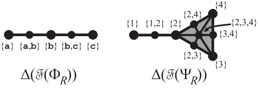
Figure 4: Order complexes of the face posets of the complexes $\Phi_{R}$ and $\Psi_{R}$ shown in Figure 3.

Viewed in the order complexes, functions $\psi_{R}$ and $\phi_{R}$ are easy to visualize. They are fully determined by their actions on vertices of the order complexes, as shown in Table 1. (Bear in mind that each element of ${\mathfrak{F}}(\Phi_{R})$ represents a simplex in $\Phi_{R}$ but is a vertex in $\Delta({\mathfrak{F}}(\Phi_{R}))$. Similarly, each element of ${\mathfrak{F}}(\Psi_{R})$ represents a simplex in $\Psi_{R}$ but is a vertex in $\Delta({\mathfrak{F}}(\Psi_{R}))$.)

$$\begin{array}[]{ccccc}\gamma&&\psi_{R}(\gamma)&&(\phi_{R}\circ\psi_{R})(\gamma)\\[1.5pt] \hline\cr\{{\tt a}\}&&\{1\}&&\{{\tt a},{\tt b}\}\\[1.5pt] \{{\tt b}\}&&\{1,2\}&&\{{\tt b}\}\\[1.5pt] \{{\tt c}\}&&\{2,3,4\}&&\{{\tt c}\}\\[1.5pt] \{{\tt a},{\tt b}\}&&\{1\}&&\{{\tt a},{\tt b}\}\\[1.5pt] \{{\tt b},{\tt c}\}&&\{2\}&&\{{\tt b},{\tt c}\}\\[1.0pt] \end{array}\hskip 43.36243pt\begin{array}[]{ccccc}\sigma&&\phi_{R}(\sigma)&&(\psi_{R}\circ\phi_{R})(\sigma)\\[1.5pt] \hline\cr\{1\}&&\{{\tt a},{\tt b}\}&&\{1\}\\[1.5pt] \{2\}&&\{{\tt b},{\tt c}\}&&\{2\}\\[1.5pt] \{3\}&&\{{\tt c}\}&&\{2,3,4\}\\[1.5pt] \{4\}&&\{{\tt c}\}&&\{2,3,4\}\\[1.5pt] \{1,2\}&&\{{\tt b}\}&&\{1,2\}\\[1.5pt] \{2,3\}&&\{{\tt c}\}&&\{2,3,4\}\\[1.5pt] \{3,4\}&&\{{\tt c}\}&&\{2,3,4\}\\[1.5pt] \{2,4\}&&\{{\tt c}\}&&\{2,3,4\}\\[1.5pt] \{2,3,4\}&&\{{\tt c}\}&&\{2,3,4\}\\[1.0pt] \end{array}$$

Table 1: The maps $\psi_{R}$ and $\phi_{R}$, and their compositions, for relation $R$ of Figure 3.

Using Table 1, one can again see how privacy loss might occur via $R$.

For instance, the map $\phi_{R}\circ\psi_{R}$ gives rise to the closure (i.e., a “pushing up”)

$$\{{\tt a}\}\xmapsto{\hskip 0.2pt\,{\psi_{R}}\hskip 0.2pt}\{1\}\xmapsto{\hskip 0.2pt\,{\phi_{R}}\hskip 0.2pt}\{{\tt a},{\tt b}\},$$

telling us how to infer unobserved attribute b from observed attribute a (in the health study example of Section 3.1, Alice could infer that Bob has_cancer from knowing that he smokes).

Similarly, for the map $\psi_{R}\circ\phi_{R}$,

$$\{4\}\xmapsto{\hskip 0.2pt\,{\phi_{R}}\hskip 0.2pt}\{{\tt c}\}\xmapsto{\hskip 0.2pt\,{\psi_{R}}\hskip 0.2pt}\{2,3,4\},$$

leading to association inference (in the payroll example from Section 3.2, the payroll clerk could infer Bob and Mary’s exposure to valuable information after learning of Julie’s work on an important project).

Figure 5 indicates the homotopy deformations produced by the maps $\phi_{R}\circ\psi_{R}$ and $\psi_{R}\circ\phi_{R}$, while Figure 6 shows the resulting image of each face poset.

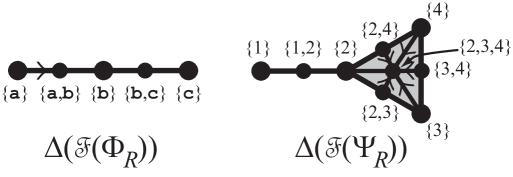
Figure 5: Closure operators $\phi_{R}\circ\psi_{R}$ and $\psi_{R}\circ\phi_{R}$ produce homotopy deformations, indicated by directed edges. In ${\mathfrak{F}}(\Phi_{R})$, $\{{\tt a}\}$ closes up to $\{{\tt a},{\tt b}\}$. In ${\mathfrak{F}}(\Psi_{R})$, most of the subsets of $\{2,3,4\}$ close up to $\{2,3,4\}$. The exception is subset $\{2\}$, which does not move.

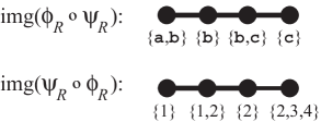
Figure 6: Images of the closure operators of Figure 5.

Observe that these two images are isomorphic. Matching up corresponding elements produces the poset $P_{R}$ of Figure 1.

Summary:

A relation $R$ produces two simplicial complexes, $\Phi_{R}$ and $\Psi_{R}$, one modeling attributes shared by individuals, the other modeling individuals with common attributes. The complexes are related by two maps, $\phi_{R}$ and $\psi_{R}$, that are homotopy inverses. The compositions of these maps describe the attribute and association inferences possible via $R$, leveraging background information someone may have. These inferences are summarized by a poset $P_{R}$ that pairs sets of individuals with sets of attributes. We may describe $P_{R}$ as follows:

Definition 3 (Doubly-Labeled Poset).

Let $R$ be a relation with nonvoid Dowker complexes.

The doubly-labeled poset $P_{R}$ associated with $R$ consists of all ordered pairs of sets $(\sigma,\gamma)$ such that $\emptyset\neq\sigma\in\Psi_{R}$, $\,\emptyset\neq\gamma\in\Phi_{R}$, $\,\sigma=\psi_{R}(\gamma)$, and $\gamma=\phi_{R}(\sigma)$.  

The partial order on $P_{R}$ is defined by: $(\sigma_{1},\gamma_{1})\leq(\sigma_{2},\gamma_{2})$ if and only if $\hbox{\hskip 1.0pt}\sigma_{1}\subseteq\sigma_{2}$

(and/or, equivalently, $\gamma_{1}\supseteq\gamma_{2}$).

See Appendix • ‣ A.4, specifically page • ‣ A.4, for some special cases.

(This definition agrees with the intuition that $P_{R}$ is both the image $(\psi_{R}\circ\phi_{R})({\mathfrak{F}}(\Psi_{R}))$ and the image $(\phi_{R}\circ\psi_{R})({\mathfrak{F}}(\Phi_{R}))$, by Appendix B.)

4.3 Attribute and Association Privacy

Here are formal definitions for the intuition developed via the previous examples:

Definition 4 (Attribute Privacy).

Let $R$ be a relation with nonvoid Dowker complexes.

We say that $R$ preserves attribute privacy precisely when
      $\phi_{R}\circ\psi_{R}$ is the identity operator on the poset  ${\mathfrak{F}}(\Phi_{R})\cup\{\emptyset\}$.

Definition 5 (Association Privacy).

Let $R$ be a relation with nonvoid Dowker complexes.

We say that $R$ preserves association privacy precisely when
      $\psi_{R}\circ\phi_{R}$ is the identity operator on the poset  ${\mathfrak{F}}(\Psi_{R})\cup\{\emptyset\}$.

Comment:

For notational simplicity, we frequently say simply that

$\phi_{R}\circ\psi_{R}$ is the identity on $\Phi_{R}$  and/or that  $\psi_{R}\circ\phi_{R}$ is the identity on $\Psi_{R}$.

4.4 Disinformation Example Re-Revisited

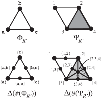
Figure 7: The Dowker complexes, as well as the order complexes of their face posets, for the relation $R^{\prime}$ of Figure 2 on page 2. The closure operator $\phi_{R^{\prime}}\circ\psi_{R^{\prime}}$ is the identity on ${\mathfrak{F}}(\Phi_{R^{\prime}})$. The closure operator $\psi_{R^{\prime}}\circ\phi_{R^{\prime}}$ on ${\mathfrak{F}}(\Psi_{R^{\prime}})$ closes many (but not all) subsets of $\{2,3,4\}$ up to $\{2,3,4\}$, as indicated by the directed arrows. The result is a poset isomorphic to the poset $P_{R^{\prime}}$ of Figure 2, drawn again slightly differently in Figure 8. Also, $(\phi_{R^{\prime}}\circ\psi_{R^{\prime}})(\emptyset)=\emptyset$. Thus relation $R^{\prime}$ preserves attribute privacy but not association privacy.

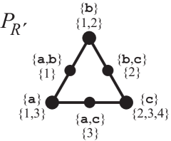
Figure 8: A flattened view of the doubly-labeled poset $P_{R^{\prime}}$ from Figure 2. Combined with Figure 7, this perspective shows how $P_{R^{\prime}}$ arises as the images of ${\mathfrak{F}}(\Phi_{R^{\prime}})$ and ${\mathfrak{F}}(\Psi_{R^{\prime}})$ under the closure operators $\phi_{R^{\prime}}\circ\psi_{R^{\prime}}$ and $\psi_{R^{\prime}}\circ\phi_{R^{\prime}}$, respectively. (The vertices drawn as bigger dots in the current figure were higher up in the poset of Figure 2 than those drawn as smaller dots.)

Recall the relation $R^{\prime}$ of Figure 2 on page 2, which is relation $R$ of Figure 1 but with an added entry of disinformation. Figure 7 displays the resulting Dowker complexes and the actions of the closure operators. Figure 8 flattens out the poset $P_{R^{\prime}}$ of Figure 2, so one sees its triangle structure and how it is the image of the Dowker complexes under the closure operators for $R^{\prime}$.

5 The Face Shape of Privacy

$\begin{array}[]{c|ccc}R&{\tt a}&{\tt b}&{\tt c}\\[2.0pt] \hline\cr 1&\bullet&\bullet&\\ 2&&\bullet&\bullet\\ 3&&&\bullet\\ 4&&&\bullet\\ \end{array}$

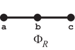
$\begin{array}[]{c|ccc}R^{\prime}&{\tt a}&{\tt b}&{\tt c}\\[2.0pt] \hline\cr 1&\bullet&\bullet&\\ 2&&\bullet&\bullet\\ 3&\bullet&&\bullet\\ 4&&&\bullet\\ \end{array}$

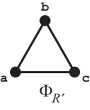
Figure 9: Relations $R$ and $R^{\prime}$ of Section 3, along with their attribute complexes $\Phi_{R}$ and $\Phi_{R^{\prime}}$.

5.1 Free Faces

Figure 9 recapitulates relation $R$ and $R^{\prime}$ from the previous two sections, along with their Dowker attribute complexes, $\Phi_{R}$ and $\Phi_{R^{\prime}}$, respectively. Recall that in $R$ one could make the inference ${\tt a}\Rightarrow{\tt b}$, but no such inference was possible in $R^{\prime}$.

The structure of $\Phi_{R}$ suggests that the inference $\,{\tt a}\Rightarrow{\tt b}\,$ might  be possible in $R$. In contrast, the structure of $\Phi_{R^{\prime}}$ makes clear that such an inference is impossible in $R^{\prime}$. In particular, observe how vertex a has only one incident edge in $\Phi_{R}$ but has two incident edges in $\Phi_{R^{\prime}}$. The fact that there are two edges in $\Phi_{R^{\prime}}$, with those edges being maximal simplices, means, intuitively, that vertex a is being “pulled” in two different inference directions, so one cannot conclude anything additional from attribute a. In contrast, in $\Phi_{R}$, vertex a is being “pulled” only toward b, so it is plausible that attribute a might imply attribute b.

The underlying geometry is that of a free face. A simplex $\gamma$ of a simplicial complex $\Gamma$ is said to be a free face of $\hbox{\hskip 1.0pt}\Gamma\hbox{\hskip 1.0pt}$ if it is a proper subset of exactly one maximal simplex of $\Gamma$. That is true for $\{{\tt a}\}$ in $\Phi_{R}$ but not for $\{{\tt a}\}$ in $\Phi_{R^{\prime}}$.

Of course, vertex $\{{\tt c}\}$ also forms a free face in $\Phi_{R}$, yet one cannot make any inferences upon observing just attribute c. What is going on? The difference is that c is also an attribute of individuals in $R\hbox{\hskip 1.0pt}$ who have only  c as an attribute (specifically, individuals #3 and #4). Even though $\{{\tt c}\}$ is technically a free face of $\Phi_{R}$, it is not really free to move under the closure operator $\phi_{R}\circ\psi_{R}$, whereas $\{{\tt a}\}$ is.

Observe that individuals #2, #3, and #4 all have attribute c, but only individual #2 has additional attributes. This means that individuals #3 and #4 cannot ever be identified uniquely in the context of relation $R$; they have effectively “camouflaged” themselves with individual #2, as far as relation $R\hbox{\hskip 1.0pt}$ is concerned. If one disallows or disregards such camouflage, then the idea of a free face and privacy loss are equivalent. The following definition is useful:

Definition 6 (Unique Identifiability).

Let $R$ be a relation on ${X}\mskip-1.8mu\times{Y}$ and suppose $x\in X$.
We say that $x$ is  uniquely identifiable via relation $R$  when $\,\psi_{R}(Y_{x})=\{x\}$.

Suppose $R\hbox{\hskip 1.0pt}$ is a relation. Appendix C.3 proves that if $\Phi_{R}$ has no free faces, then $R\hbox{\hskip 0.2pt}$ preserves attribute privacy. For the converse, Appendix C.3 further proves that if $R$ preserves attribute privacy ​and if every individual is uniquely identifiable, then $\Phi_{R}$ has no free faces. (Dual statements hold for association privacy.)

5.2 Privacy versus Identifiability

Section 5.1 hinted at the difference between privacy and identifiability. In relation $I$ below (“I” for “individuality” or “identity”), every individual has exactly one attribute and that attribute uniquely identifies the individual. Relation $I$ preserves privacy fully (assuming $n>1$). It is impossible to make any attribute inferences. If Bob reveals that he has attribute $y_{7}$, then Alice cannot infer any additional attributes for Bob. She now knows that Bob is individual $x_{7}$ but cannot infer any additional attributes. He has himself revealed everything about himself that there is to know, as far as relation $I$ is concerned.

$$\begin{array}[]{c|cccccc}I&y_{1}&y_{2}&\cdots&y_{n}\\[2.0pt] \hline\cr x_{1}&\bullet&&&\\ x_{2}&&\bullet&&\\ \vdots&&&\ddots&\\ x_{n}&&&&\bullet\\ \end{array}$$

In contrast, all individuals in relation $C$ (for “conformism” or “confusion”) have exactly the same set of attributes. As a result, there is no privacy: one can predict all the attributes of any individual in the relation without making any observations. On the other hand, no individual is uniquely identifiable (assuming $n>1$).

$$\begin{array}[]{c|cccccc}C&y_{1}&y_{2}&\cdots&y_{n}\\[2.0pt] \hline\cr x_{1}&\bullet&\bullet&\cdots&\bullet\\ x_{2}&\bullet&\bullet&\cdots&\bullet\\ \vdots&\vdots&\vdots&\ddots&\vdots\\ x_{n}&\bullet&\bullet&\cdots&\bullet\\ \end{array}$$

Homogeneity:

Relation $C$ exhibits a form of homogeneity often sought by anonymization or other privacy techniques. As we have suggested before, the utility of relation $C$ is essentially zero, unless one makes the entries stochastic, so that some utility is encoded in the distribution.

The discussion of free faces in Section 5.1 suggests an alternative approach to homogeneity: one may preserve privacy and retain utility by choosing the geometry of the relation appropriately, for instance, so the space $\Phi_{R}$ exhibits sphere-like homogeneity. There will be considerable discussion of the importance of spheres in the rest of the report.

5.3 Spheres and Privacy

The attribute complex $\Phi_{R^{\prime}}$ of Figure 9 is equal to a boundary complex, namely the boundary of the full simplex consisting of the attributes $\{{\tt a},{\tt b},{\tt c}\}$. We will denote boundary complexes by ${\partial{(V)}}$, with $V$ some nonempty set. The simplices of ${\partial{(V)}}$ are all proper subsets of $V$. Boundary complexes are homotopic to spheres, specifically ${\partial{(V)}}\simeq\mathbb{S}^{\kern 0.56001pt{n-2}}$, with $n=\lvert V\rvert$. For $\Phi_{R^{\prime}}$ of Figure 9, we have that $\Phi_{R^{\prime}}={\partial{(\{{\tt a},{\tt b},{\tt c}\})}}\simeq\,\mathbb{S}^{1}$. (In English: The Dowker attribute complex is the boundary of a triangle, so homotopic to a circle.)

More generally, if for some relation $R$ on ${X}\mskip-1.8mu\times{Y}$, $\Phi_{R}={\partial{(Y)}}$, then $\Phi_{R}$ cannot have any free faces and so $R$ preserves attribute privacy.

Privacy and Utility:

An important observation is that boundary complexes exhibit homogeneity but still permit identifiability. If $\Phi_{R}={\partial{(Y)}}$, with $\lvert Y\rvert>1$, and if no individual’s attributes are a subset of another’s attributes, then one can and needs to specify $\lvert Y\rvert-1$ attributes in order to identify an individual. The boundary structure ensures that one cannot infer any attributes by specifying fewer than $\lvert Y\rvert-1$ attributes, yet retains the ability to identify every individual.

Appendix J.1 gives an example of a contractible space that preserves attribute privacy. Observe, however, that the number of attributes needed to identify an individual in that example is considerably less than the total number of attributes in the space. For a boundary complex, it is just one less.

Preserving Attribute and Association Privacy:

A consequence of these observations is that if one wishes to preserve both attribute and association privacy with a connected relation, then one requires both Dowker complexes to look like spheres. More specifically, either both Dowker complexes are linear cycles of the same length or both are boundary complexes of the same dimension. In the latter case, the relation is isomorphic to a relation of the following form, in which the diagonal $\{(x_{i},y_{i})\}$ is blank but all other entries are present:

$$\begin{array}[]{c|cccccc}R&y_{1}&y_{2}&\cdots&\cdots&y_{n-1}&y_{n}\\[2.0pt] \hline\cr x_{1}&&\bullet&\bullet&\cdots&\bullet&\bullet\\ x_{2}&\bullet&&\bullet&\cdots&\bullet&\bullet\\ \vdots&\bullet&\bullet&&\ddots&\vdots&\bullet\\ \vdots&\vdots&\vdots&\ddots&&\bullet&\vdots\\ x_{n-1}&\bullet&\bullet&\cdots&\bullet&&\bullet\\ x_{n}&\bullet&\bullet&\bullet&\cdots&\bullet&\\ \end{array}$$

See Appendix E.3, starting on page E.3, for further details.

5.4 A Spherical Non-Boundary Relation that Preserves Attribute Privacy

$\begin{array}[]{c|ccccc}R&{\tt a}&{\tt b}&{\tt c}&{\tt d}&{\tt e}\\[2.0pt] \hline\cr 1&\bullet&\bullet&&\bullet&\\ 2&\bullet&&\bullet&\bullet&\\ 3&&\bullet&\bullet&\bullet&\\ 4&\bullet&\bullet&&&\bullet\\ 5&\bullet&&\bullet&&\bullet\\ 6&&\bullet&\bullet&&\bullet\\ \end{array}$

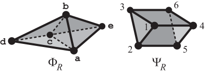
Figure 10: A relation $R$ and its Dowker complexes $\Phi_{R}$ and $\Psi_{R}$, each homotopic to the two-dimensional sphere $\mathbb{S}^{2}$. (One may view $\Phi_{R}$ as two party hats glued together. One may view $\Psi_{R}$ as a cylinder with a triangular cross-section and endcaps. However, the quadrilaterals drawn for the cylinder portion of $\Psi_{R}$ are simply flattened sketches of what are actually solid tetrahedra.)

Consider relation $R$ as in Figure 10. Relation $R$ preserves attribute privacy, since $\Phi_{R}$ has no free faces. The relation does not preserve association privacy. In particular, the quadrilaterals drawn for $\Psi_{R}$ in the figure are actually tetrahedra. This means that the diagonals of the quadrilaterals are free faces. For instance, one would expect to infer individuals #1 and #6 as additional unobserved associates if one observes individuals #3 and #4. Indeed, computing using the closure operator $\psi_{R}\circ\phi_{R}$, we see that:

$$(\psi_{R}\circ\phi_{R})(\{3,4\})\;=\;\psi_{R}(\{{\tt b}\})\;=\;\{1,3,4,6\}.$$

Relation $R$ has another interesting feature. Even though $\Phi_{R}$ is not itself a boundary complex, it is the simplicial join (see page • ‣ A.1) of two boundary complexes:

$$\Phi_{R}\;=\;{\partial{(\{{\tt a},{\tt b},{\tt c}\})}}*{\partial{(\{{\tt d},{\tt e}\})}}.$$

In fact, we can think of $R$ as $R_{1}\cup R_{2}$ and $\Phi_{R}$ as $\Phi_{R_{1}}\mskip-1.5mu*\mskip 1.5mu\Phi_{R_{2}}$, with $R_{1}$ the restriction of $R$ to the attributes $\{{\tt a},{\tt b},{\tt c}\}$ and $R_{2}$ the restriction of $R$ to the attributes $\{{\tt d},{\tt e}\}$. This join structure of $\Phi_{R}$ means that we can view every individual in $R$ as being described by two independent attribute spaces. The attribute space $\{{\tt d},{\tt e}\}$ acts like a standard bit; every individual has exactly one of these two attributes. In contrast, the attribute space $\{{\tt a},{\tt b},{\tt c}\}$ is an “any 2 of 3” type of descriptor. Every individual has exactly two of these three attributes.

Figure 11 shows the relations $R_{1}$ and $R_{2}$ along with their Dowker attribute complexes.

$\begin{array}[]{c|ccc}R_{1}&{\tt a}&{\tt b}&{\tt c}\\[2.0pt] \hline\cr 1&\bullet&\bullet&\\ 2&\bullet&&\bullet\\ 3&&\bullet&\bullet\\ 4&\bullet&\bullet&\\ 5&\bullet&&\bullet\\ 6&&\bullet&\bullet\\ \end{array}$

$\begin{array}[]{c|cc}R_{2}&{\tt d}&{\tt e}\\[2.0pt] \hline\cr 1&\bullet&\\ 2&\bullet&\\ 3&\bullet&\\ 4&&\bullet\\ 5&&\bullet\\ 6&&\bullet\\ \end{array}$

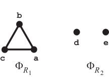
Figure 11: Relation $R$ of Figure 10 decomposes into two disjoint relations $R_{1}$ and $R_{2}$ such that $\Phi_{R}=\Phi_{R_{1}}\mskip-1.5mu*\mskip 1.5mu\Phi_{R_{2}}$, with $\Phi_{R_{1}}$ the boundary complex of a triangle and $\Phi_{R_{2}}$ two isolated points. This means every individual in $R$ has attributes that act like two independent coordinates: an “any 2 of 3” component and a bit.

6 Conditional Relations as Simplicial Links

The decomposition of Figures 10 and 11 is reminiscent of stochastic independence expressed as multiplication of probabilities. Similarly, there is a combinatorial analogue to the notion of a conditional probability distribution. It appears as the link  of a simplex in a simplicial complex.

Given a relation $R$, suppose we have observed attributes $\gamma$ for some unknown individual. The remaining possible combinations of attributes we might yet observe are described by the simplicial complex $\mathop{\rm Lk}(\Phi_{R},\gamma)={\left\{\tau\in\Phi_{R}\;\left|\;\tau\cap\gamma=\emptyset\;\hbox{and}\;\tau\cup\gamma\in\Phi_{R}\right.\right\}}$. Interpretation: $\tau\cap\gamma=\emptyset$ means that $\tau$ consists of as yet unobserved attributes, while $\tau\cup\gamma\in\Phi_{R}$ means that there is some individual who has the attributes $\tau$ in addition to the attributes $\gamma$ that we have already observed.

$\begin{array}[]{c|ccc}Q&{\tt a}&{\tt b}&{\tt c}\\[2.0pt] \hline\cr 1&\bullet&\bullet&\\ 2&\bullet&&\bullet\\ 3&&\bullet&\bullet\\ \end{array}$

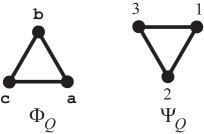
Figure 12: Relation $Q$ describes the conditional relation resulting from $R$ of Figure 10 upon observing attribute d. Note that $\Phi_{Q}=\mathop{\rm Lk}(\Phi_{R},\{{\tt d}\})$.

For instance, after observing attribute d in relation $R$ of Figure 10, we may conclude that we are observing one of the individuals in $\{1,2,3\}$ and that the remaining attributes we might yet observe are any two attributes drawn from $\{{\tt a},{\tt b},{\tt c}\}$. We can express these conclusions as yet another relation, namely the relation $Q$ of Figure 12. Relation $Q$ describes exactly which individuals could give rise to which attributes, consistent with the prior observation of attribute d. Thus $\Phi_{R}$ plays a role much like a probability distribution, while $\Phi_{Q}$ plays the role of a conditional distribution. For another example, suppose we have observed attribute b in $R$. Then the resulting conditional relation $Q^{\prime}$ is as in Figure 13.

$\begin{array}[]{c|cccc}Q^{\prime}&{\tt a}&{\tt c}&{\tt d}&{\tt e}\\[2.0pt] \hline\cr 1&\bullet&&\bullet&\\ 3&&\bullet&\bullet&\\ 4&\bullet&&&\bullet\\ 6&&\bullet&&\bullet\\ \end{array}$

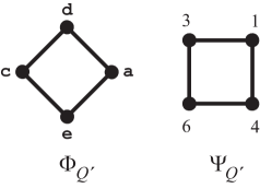
Figure 13: Relation $Q^{\prime}$ describes the conditional relation resulting from $R$ of Figure 10 upon observing attribute b. Here $\Phi_{Q^{\prime}}=\mathop{\rm Lk}(\Phi_{R},\{{\tt b}\})$. Observe that the attribute space for $Q^{\prime}$ now factors into two independent bits: $\{{\tt a},{\tt c}\}$ constitutes one bit, $\{{\tt d},{\tt e}\}$ the other. This factoring is conditional  on having observed b.

The formal constructions of conditional relations appear below.  See also Appendix C.1.

Notation:

A symbol of the form $R|_{W}$ means “restrict $R$ to $W$”. For instance, if $R$ is a relation on ${X}\mskip-1.8mu\times{Y}$, and if $A\subseteq X$ and $B\subseteq Y$, then  $R|_{A\times B}\;=\;R\,\cap(A\times B)$.

Definition 7 (Conditional Attribute Relations).

Let $R$ be a nonvoid relation on ${X}\mskip-1.8mu\times{Y}$ and suppose $\gamma\subseteq Y$.  The following relation $Q$ models $\mathop{\rm Lk}(\Phi_{R},\gamma)$:

$$Q\;=\;R\,|_{\sigma\times\overline{Y}},\quad\hbox{with}\quad\sigma=\psi_{R}(\gamma)\quad\hbox{and}\quad\overline{Y}=\bigcup_{x\in\sigma}Y_{x}\setminus\gamma.\phantom{00000}$$

The Dowker complexes are defined in the standard way, except for this special case:

If $\,\overline{Y}=\emptyset$ and $\sigma\neq\emptyset$, then we let $\Phi_{Q}$ and $\Psi_{Q}$ be instances of the empty complex $\{\emptyset\}$.

Observe:

$\mathop{\rm Lk}(\Phi_{R},\gamma)=\Phi_{Q}$  (a proof appears in Appendix C.1, on page C.1).

Comment:

If $\gamma\not\in\Phi_{R}$, then $\sigma=\emptyset$ and $Q$ is void, and so $\Phi_{Q}$ is an instance of the void complex, consistent with the standard definition of $\mathop{\rm Lk}(\Phi_{R},\gamma)$ being void in this situation.  (See page A.1 in Appendix A.1 for the definitions of void simplicial complex  and empty simplicial complex, and page A.4 in Appendix A.4 for the definition of void relation.)

There is a dual construction for links of individuals $\sigma$ in the Dowker complex modeling associations:

Definition 8 (Conditional Association Relations).

Let $R$ be a nonvoid relation on ${X}\mskip-1.8mu\times{Y}$ and suppose $\sigma\subseteq X$.  The following relation $Q$ models $\mathop{\rm Lk}(\Psi_{R},\sigma)$:

$$Q\;=\;R\,|_{\overline{X}\times\gamma},\quad\hbox{with}\quad\gamma=\phi_{R}(\sigma)\quad\hbox{and}\quad\overline{X}=\bigcup_{y\in\gamma}X_{y}\setminus\sigma.\phantom{00000}$$

The Dowker complexes are defined in the standard way, except for this special case:

If $\,\overline{X}=\emptyset$ and $\gamma\neq\emptyset$, then we let $\Psi_{Q}$ and $\Phi_{Q}$ be instances of the empty complex $\{\emptyset\}$.

Observe:

$\mathop{\rm Lk}(\Psi_{R},\sigma)=\Psi_{Q}$.

As we will see in Section 7, the complex $\mathop{\rm Lk}(\Psi_{R},\{x\})$ is useful for characterizing individual $x$’s attribute privacy. If that seems surprising, observe that $\mathop{\rm Lk}(\Psi_{R},\{x\})$ describes other individuals in $R$ who share attributes with $x$, with simplices modeling the extent of commonalities. These commonalities, or lack thereof, determine whether in $\Phi_{Q}$, and thus back in $\Phi_{R}$, there are attributes of $x$ that are “free to move” under the closure operators.

7 Privacy Characterization via Boundary Complexes

$\begin{array}[]{c|ccccc}Q&{\tt b}&{\tt c}&{\tt d}\\[2.0pt] \hline\cr 1&\bullet&&\bullet\\ 2&&\bullet&\bullet\\ 4&\bullet&&\\ 5&&\bullet&\\ 6&\bullet&\bullet&\\ \end{array}$

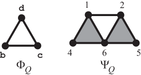
Figure 14: With $R$ as in Figure 10, relation $Q$ describes the conditional relation corresponding to $\mathop{\rm Lk}(\Psi_{R},\{3\})$. Also shown are the Dowker complexes of $Q$. By design, $\Psi_{Q}=\mathop{\rm Lk}(\Psi_{R},\{3\})$. Observe that $\Phi_{Q}$ is the boundary complex ${\partial{(\{{\tt b},{\tt c},{\tt d}\})}}$, with $\{{\tt b},{\tt c},{\tt d}\}$ being all of individual #3’s attributes in relation $R$. That boundary condition characterizes attribute privacy for an identifiable individual.  Here, it means that individual #3 has full attribute privacy.

We observed earlier that relation $R$ of Figure 10 preserves attribute privacy. We came to that conclusion after observing that $\Phi_{R}$ has no free faces. In fact, one can focus on the privacy of any identifiable individual rather than look at the whole relation. Let us pick one such individual, say #3, and look at the conditional relation $Q$ that models the link $\mathop{\rm Lk}(\Psi_{R},\{3\})$, as shown in Figure 14.  (Observe that individual #3 is indeed uniquely identifiable via $R$.)

Individual #3 has attributes $\{{\tt b},{\tt c},{\tt d}\}$ in $R$. The attribute complex $\Phi_{Q}$ for $Q$ is the boundary complex on exactly this set. Interpretation: for any nonempty proper subset of individual #3’s attributes, some  other  individual in $R\hbox{\hskip 1.0pt}$ has at least those attributes but not all of individual #3’s attributes. Consequently, there is a different such individual for each proper subset of $\{{\tt b},{\tt c},{\tt d}\}$ that is missing exactly one of #3’s attributes. That diversity of individuals ensures individual #3’s attribute privacy.

The previous example suggests the following characterization: An identifiable individual has full attribute privacy precisely when the attribute complex of the individual’s link is the boundary complex of the individual’s attributes.

Observe that this characterization is local to the individual; it does not depend on other individuals having privacy.  We now formalize this intuition.  Proofs appear in Appendix E.

First, a definition to make precise the notion of individual privacy:

Definition 9 (Individual Privacy).

Let $R$ be a relation on ${X}\mskip-1.8mu\times{Y}$ and suppose $x\in X$.

We say that $R$ preserves attribute privacy for $x$ whenever $(\phi_{R}\circ\psi_{R})(\gamma)=\gamma$ for all $\gamma\subseteq Y_{x}$.

Informally, we may also say that  individual $x$ has full attribute privacy.

Recall also Definitions 4 and 6, from pages 4 and 6, respectively, formalizing the notions of (attribute) privacy preservation and unique identifiability. And recall the semantics of $P_{R}$, for instance from Definition 3 on page 3.

Here is the characterization of individual attribute privacy formalized:

Theorem 10 (Individual Attribute Privacy).

Let $R$ be a relation on ${X}\mskip-1.8mu\times{Y}$, with $\lvert X\rvert>1$. Suppose $x\in X$ is uniquely identifiable via $R$.  Let $Q$ be the relation modeling $\mathop{\rm Lk}(\Psi_{R},x)$.
Then the following three conditions are equivalent:

1. $R$ preserves attribute privacy for $x$.

2. $\mathop{\rm Lk}(\Psi_{R},x)\;\simeq\;\,\mathbb{S}^{\kern 0.56001pt{k-2}}$, with $k=\lvert Y_{x}\rvert$.

3. $\Phi_{Q}\;=\;\partial(Y_{x})$.

The previous theorem generalizes to sets of individuals for sets that are “stable” under the closure operators, i.e., that appear as the “set of individuals component” in an element of $P_{R}$:

Theorem 11 (Group Attribute Privacy).

Let $R$ be a relation on ${X}\mskip-1.8mu\times{Y}$.
Suppose $(\sigma,\gamma)\in P_{R}$, with $\sigma\neq X$.  Let $Q$ be the relation modeling $\mathop{\rm Lk}(\Psi_{R},\sigma)$.
Then the following three conditions are equivalent:

1. $(\phi_{R}\circ\psi_{R})(\gamma^{\prime})\;=\;\gamma^{\prime}$, for every subset $\gamma^{\prime}$ of $\gamma$.

2. $\mathop{\rm Lk}(\Psi_{R},\sigma)\;\simeq\;\mathbb{S}^{\kern 0.56001pt{k-2}}$, with $k=\lvert\gamma\rvert$.

3. $\Phi_{Q}\;=\;\partial(\gamma)$.

The following lemma relates interpretation and inference in a link to the encompassing relation:

Lemma 12 (Interpreting Local Operators).

Let $R$ be a relation on ${X}\mskip-1.8mu\times{Y}$.

Suppose $(\sigma,\gamma)\in P_{R}$, with $\sigma\neq X$.

Let $Q$ be the relation on $\overline{X}\times\gamma$ that models $\mathop{\rm Lk}(\Psi_{R},\sigma)$ and suppose $\overline{X}\neq\emptyset$.  

Then, for every $\gamma^{\prime}\subseteq\gamma$:

1. If $\,\gamma^{\prime}\not\in\Phi_{Q}$, then $\psi_{R}(\gamma^{\prime})=\sigma$.

2. If $\,\gamma^{\prime}\in\Phi_{Q}$, then $\psi_{R}(\gamma^{\prime})\supsetneq\sigma$.

   Moreover, in this case:

   For $\,\gamma^{\prime}=\emptyset$,  $(\phi_{Q}\circ\psi_{Q})(\emptyset)\supseteq(\phi_{R}\circ\psi_{R})(\emptyset)$.

   If $\,\gamma^{\prime}\neq\emptyset$,  then $(\phi_{Q}\circ\psi_{Q})(\gamma^{\prime})=(\phi_{R}\circ\psi_{R})(\gamma^{\prime})$.

The lemma says that observations of attributes consistent in $Q$ have as interpretation more individuals in $R$ than just the individuals $\sigma$. However, if ever those observations become inconsistent in $Q$, then one has identified $\sigma$ in $R$. Here “inconsistent in $Q$” means that the observed attributes are legitimate attributes for $Q$ but do not constitute a simplex of $\Phi_{Q}$. (Note: Such observed attributes necessarily constitute a simplex of $\Phi_{R}$ since they are a subset of $\gamma\in\Phi_{R}$).

Moreover, attribute inferences are identical in $Q$ and $R$ for nonempty simplices of $\Phi_{Q}$.

8 The Meaning of Holes in Relations

We have seen how spheres characterize privacy. More generally, when working with topological spaces, holes are significant. One wonders what topological holes mean for relations.

• Some holes arise as a consequence of exclusion between attributes, as we saw in the decomposition of Figures 10 and 11.

  Sticking with binary exclusions, suppose a group of individuals are described by $k$ bits. One can model those individuals via a relation containing $2k$ binary attributes (two such attributes per bit, one for each possible bit value). Every individual has exactly $k$ of those $2k$ attributes. If all possible $2^{k}$ combinations of bit values are represented by individuals in the relation, then the two Dowker complexes are both homotopic to $\mathbb{S}^{\kern 0.56001pt{k-1}}$, the sphere of dimension $k-1$. In fact, $\Phi_{R}$ is the simplicial join of $k$ copies of $\mathbb{S}^{\kern 0.56001pt{0}}$, while $\Psi_{R}$ is visualizable as a hollow hypercube in $k$ dimensions, in which solid ($k-1$)-dimensional subcubes represent $(2^{k-1}-1)$-dimensional simplices (flattened, when $k\geq 3$). Figures 15, 16, and 17 depict the cases $k=1$, 2, and 3, respectively.

  In short, $k$ bits means a hole of dimension $k$$-$$1$, if  all possible individuals are actually present in the relation.

  (The lack of an expected hole may mean that the capacity of a relation has not been exhausted, hinting at possible inference. See Appendix J.3.)

  $\begin{array}[]{c|cccc}\hbox{\large$S$}&{\tt a}&\neg{\tt a}\\[2.0pt] \hline\cr 1&\bullet&\\ 2&&\bullet\\ \end{array}$

  

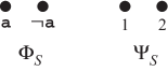
  Figure 15: Relation $S$ describes two individuals in terms of a single attribute and its negation. The topology of the Dowker complexes is $\mathbb{S}^{\kern 0.56001pt{0}}$.

  $\begin{array}[]{c|cccc}\hbox{\large$Q$}&{\tt a}&\neg{\tt a}&{\tt b}&\neg{\tt b}\\[2.0pt] \hline\cr 1&\bullet&&\bullet&\\ 2&\bullet&&&\bullet\\ 3&&\bullet&\bullet&\\ 4&&\bullet&&\bullet\\ \end{array}$

  

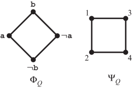
  Figure 16: Relation $Q$ describes four individuals in terms of two attributes and their negations. The topology of the Dowker complexes is $\mathbb{S}^{1}$.

  $\begin{array}[]{c|cccccc}\hbox{\large$R$}&{\tt a}&\neg{\tt a}&{\tt b}&\neg{\tt b}&{\tt c}&\neg{\tt c}\\[2.0pt] \hline\cr 1&\bullet&&\bullet&&\bullet&\\ 2&\bullet&&\bullet&&&\bullet\\ 3&\bullet&&&\bullet&\bullet&\\ 4&\bullet&&&\bullet&&\bullet\\ 5&&\bullet&\bullet&&\bullet&\\ 6&&\bullet&\bullet&&&\bullet\\ 7&&\bullet&&\bullet&\bullet&\\ 8&&\bullet&&\bullet&&\bullet\\ \end{array}$

  

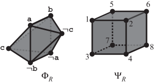
  Figure 17: Relation $R$ describes eight individuals in terms of three attributes and their negations. The topology of the Dowker complexes is $\mathbb{S}^{2}$. The cube faces are actually tetrahedra, flattened to parallelograms in the drawing.

• Suppose $\Sigma$ is a simplicial complex with underlying vertex set $X$. A minimal nonface of $\Sigma\hbox{\hskip 0.2pt}$ is a subset of $X$ that is not itself a simplex but all of whose proper subsets are simplices in $\Sigma$. A minimal nonface may or may not be a topological hole. Regardless, a minimal nonface of size two or greater in a Dowker complex suggests restricting the relation to equal-numbered attributes and individuals for whom there is both attribute and association privacy, within the restricted relation. This observation dovetails with the following results (here we assume that each relation has no blank rows or columns):

  • A relation with more attributes than individuals cannot fully preserve attribute privacy.

  • A relation with more individuals than attributes cannot fully preserve association privacy.

  • A relation that preserves both attribute and association privacy must have the same number of attributes and individuals. Moreover, if the relation is connected, then both Dowker complexes are either linear cycles of the same length or boundary complexes of full simplices of the same dimension, as we indicated previously.

  See Appendices C and E  for further details and proofs.

• Minimal nonfaces can have other context-dependent meanings. For instance, in a certain authorship relation, knowing that each pair  of three individuals has written a paper together appears to be a good predictor that all three  individuals will co-author a paper together [15]. This observation suggests the following: if one sees that such an authorship hole does not  fill over time, then one likely can infer some kind of obstruction, perhaps an incompatibility in the group as a whole, or the death of an author, for instance.

• When designing relations or anonymizing relations, these results suggest transformations that create “bubbly spaces” of some sort, in order to retain identifiability but also reduce unwanted inference. Section 9 and Appendix J.2 discuss examples.

• Whatever topological holes there are in $\Phi_{R}$ and $\Psi_{R}$ must also show up in the poset $P_{R}$, since that poset is formed by homotopy equivalences from $\Phi_{R}$ and $\Psi_{R}$. Interestingly, whereas one thinks of $\Phi_{R}$ and $\Psi_{R}$ simply as spaces, one sees a partial order on $P_{R}$. Something can move, “up” or “down”. The elements of $P_{R}$ are inference-stable, by design. So, what is this possible motion?  It is a dynamic process that describes how information acquisition changes interpretation. For instance, as an individual reveals information about him- or herself, an observer can attempt to identify the individual, by finding interpretations in $P_{R}$ of the information revealed. As the individual reveals additional information, the observer’s interpretation moves downward in $P_{R}$, narrowing the set of individuals.

  Topological holes in the spaces $\Phi_{R}$ and $\Psi_{R}$ (and thus $P_{R}$) constrain how that interpretation moves downward in $P_{R}$. The greater a hole’s dimension, the further a downward path has to move before identifying an individual. One can think of holes in a relation much like boulders in a stream. Eventually, the current of information sweeps past the hole, but it is forced to divert its motion, covering more distance. Moreover, there may be many paths around the hole, much like a leaf in a stream may divert around a boulder in different directions. The individual can force a particular path by choosing to reveal attributes in a particular order.

  Much of the rest of the report explores the implications of this stream analogy. The analogy merges with the realization that privacy is a dynamic process, certain to flow toward identification when attributes are static or persistent, yet subject to channeling (perhaps even turbulence in more fluid settings than those discussed in this report). See, in particular, Section 10 onward.

9 Change-of-Attribute Transformations

Free faces and holes in the Dowker complex $\Phi_{R}$ can sometimes suggest changes in attributes that preserve desired information but reduce inference. Consider the hypothetical “ice-cream cone” relation $C$ of Figure 18 and the corresponding complexes shown in Figure 19. The relation describes four individuals in terms of the two-flavor two-scoop ice-cream cones each individual enjoys at a particular ice-cream parlor.

$\begin{array}[]{l|cccccc}\hbox{\large$\;\;C$}&{\tt gc}&{\tt gs}&{\tt cs}&{\tt cv}&{\tt sv}&{\tt gv}\\[2.0pt] \hline\cr\hbox{Bob}&\bullet&\bullet&\bullet&&&\\ \hbox{Alice}&&&\bullet&\bullet&\bullet&\\ \hbox{David}&&\bullet&&&\bullet&\bullet\\ \hbox{Cindy}&\bullet&&&\bullet&&\bullet\\ \end{array}$

$\begin{array}[]{lcl}&&\\ {\tt g}&=&\hbox{ginger}\\ {\tt c}&=&\hbox{chocolate}\\ {\tt s}&=&\hbox{strawberry}\\ {\tt v}&=&\hbox{vanilla}\\ \end{array}$

Figure 18: Four individuals and their preferences for ice-cream cones containing two scoops, with different flavors (each letter represents a flavor, as indicated). See Figure 19 for the Dowker complexes.

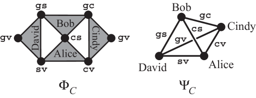
Figure 19: The Dowker complexes for the relation of Figure 18. $\Phi_{C}$ is a complex whose vertices are ice-cream cones (two flavors). (For visualization purposes, the complex is flattened, with the leftmost and rightmost vertices really representing the same ice-cream cone.) Each maximal simplex is a triangle, labeled with the individual who enjoys the three types of cones comprising the triangle. $\Psi_{C}$ is a complex whose vertices are individuals. Each maximal simplex is an edge, representing a two-flavor two-scoop ice-cream cone that each of two individuals enjoys; the edge is labeled with the cone flavors. The homotopy type of each complex is $\mathbb{S}^{1}\vee\mathbb{S}^{1}\vee\mathbb{S}^{1}$.

Relation $C$ is a typical “2-implies-3” relation: Any two different ice-cream cones uniquely identify an individual, thereby implying a third ice-cream cone, as can be seen from either Dowker complex: In $\Phi_{C}$, every edge is a free face of its encompassing triangle. Moreover, the edge is not itself generated by any individual. The closure operator $\phi_{C}\circ\psi_{C}$ must therefore map every edge to a triangle. Dually, in $\Psi_{C}$, any two edges intersecting at a vertex imply the third edge incident on that vertex.

This type of relation models, in the small, inferences such as those reported in [21, 17]. For instance, [21] reported that zip code, gender, and birth date were likely sufficient in 1990 to identify $87\%$ of individuals in the U.S. That is nearly a “3-implies-all” type of relation. Similarly, [17] reported that 8 movie ratings and dates were enough to uniquely identify $99\%$ of viewers in the Netflix Prize dataset. That is essentially an “8-implies-all” type of relation.

Let us focus for a moment on Bob’s neighborhood. That relation, let us call it $B$, and its complexes are depicted in Figure 20. (The relation models $\mathop{\rm\overline{St}}(\Psi_{C},\{\hbox{Bob}\})$; see Appendix • ‣ A.1.)

$\begin{array}[]{l|ccc}\hbox{\large$\;\;B$}&{\tt gc}&{\tt gs}&{\tt cs}\\[2.0pt] \hline\cr\hbox{Bob}&\bullet&\bullet&\bullet\\ \hbox{Alice}&&&\bullet\\ \hbox{David}&&\bullet&\\ \hbox{Cindy}&\bullet&&\\ \end{array}$

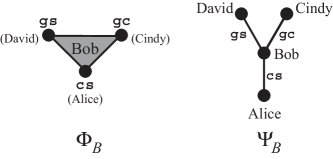
Figure 20: Relation $B$ models Bob’s neighborhood in the ice-cream relation of Figure 18. Each maximal simplex is labeled with its generator. Generators of nonmaximal simplices are indicated in parentheses.

As in $C$, seeing someone eat one ice-cream cone is not enough to identify anyone in $B$ uniquely. Seeing someone (in this case, Bob) eat two different types of ice-cream cones is sufficient to infer the third type of ice-cream cone that individual prefers. How might we prevent this? We observe that the vertices of $\Phi_{B}$ are themselves generated by individuals while the edges are not. Homotopically, therefore, we want to expand the vertices of $\Phi_{B}$ into edges, and contract the edges of $\Phi_{B}$ into vertices. One possible way to accomplish this is the take logical ors of the existing attributes. With $\oplus$ meaning Boolean or, we define:

$$\alpha\;=\;{\tt gc}\;\oplus\;{\tt gs},\qquad\beta\;=\;{\tt gc}\;\oplus\;{\tt cs},\qquad\gamma\;=\;{\tt gs}\;\oplus\;{\tt cs}.$$

Then relation $B$ becomes $B^{\prime}$ as in Figure 21. The result is that the free faces of $\Phi_{B^{\prime}}$ now are generated by other individuals, so even though they are free, the closure operator does not move them. In fact, the closure operator $\phi_{B^{\prime}}\circ\psi_{B^{\prime}}$ is the identity on ${{\mathfrak{F}}(\Phi_{B^{\prime}})\cup\{\emptyset\}}$, meaning that no attribute inference is possible in $B^{\prime}$.

$\begin{array}[]{l|ccc}\hbox{\large$\;B^{\prime}$}&\alpha&\beta&\gamma\\[2.0pt] \hline\cr\hbox{Bob}&\bullet&\bullet&\bullet\\ \hbox{Alice}&&\bullet&\bullet\\ \hbox{David}&\bullet&&\bullet\\ \hbox{Cindy}&\bullet&\bullet&\\ \end{array}$

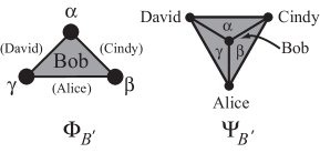
Figure 21: Relation $B^{\prime}$ represents relation $B$ of Figure 20, now with a coordinate transformation for the attributes. Simplices are again labeled by generators.

Now imagine performing similar operations for all four individuals of relation $C$ from Figure 18. One winds up constructing four logical ors:

$${\tt gc}\;\oplus\;{\tt gs}\;\oplus\;{\tt gv},\qquad{\tt gc}\;\oplus\;{\tt cs}\;\oplus\;{\tt cv},\qquad{\tt gs}\;\oplus\;{\tt cs}\;\oplus\;{\tt sv},\qquad{\tt cv}\;\oplus\;{\tt sv}\;\oplus\;{\tt gv}.$$

Two observations:

1. Each or describes three ice-cream cones that form a hole in the complex $\Phi_{C}$ of Fig. 19.

2. Each such hole may be interpreted as a single flavor, namely the flavor in common to the three ice-cream cones appearing in the or. For instance, “ginger” (abbreviated as ${\tt g}$) is the common flavor for the or  ${\tt gc}\oplus{\tt gs}\oplus{\tt gv}$.

In order to describe the resulting relation, it is perhaps easiest to express those four new coordinates themselves via a relation $S$ that describes the scoops present in an ice-cream cone:

$$\begin{array}[]{c|cccc}\hbox{\large$S$}&{\tt g}&{\tt c}&{\tt s}&{\tt v}\\[2.0pt] \hline\cr{\tt gc}&\bullet&\bullet&&\\ {\tt gs}&\bullet&&\bullet&\\ {\tt cs}&&\bullet&\bullet&\\ {\tt cv}&&\bullet&&\bullet\\ {\tt sv}&&&\bullet&\bullet\\ {\tt gv}&\bullet&&&\bullet\\ \end{array}$$

Finally, to perform the coordinate-transformation, one simply multiplies Boolean matrices, with addition being Boolean or and multiplication being Boolean and: $F=CS$. The relation $F$ and its complexes appear in Figure 22.

$\begin{array}[]{l|cccc}\hbox{\large$\;\;F$}&{\tt g}&{\tt c}&{\tt s}&{\tt v}\\[2.0pt] \hline\cr\hbox{Bob}&\bullet&\bullet&\bullet&\\ \hbox{Alice}&&\bullet&\bullet&\bullet\\ \hbox{David}&\bullet&&\bullet&\bullet\\ \hbox{Cindy}&\bullet&\bullet&&\bullet\\ \end{array}$

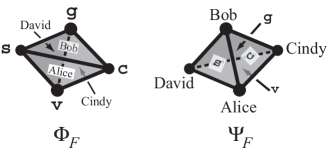
Figure 22: Relation $F$ describes the ice-cream flavors each individual prefers. $\Phi_{F}$ is the boundary complex of a tetrahedron, with flavors as vertices. $\Psi_{F}$ is the Dowker dual of $\Phi_{F}$, with respect to relation $F$. Consequently, $\Psi_{F}$ also is the boundary complex of a tetrahedron, now with the roles of flavors and individuals interchanged.  For both $\Phi_{F}$ and $\Psi_{F}$, each maximal simplex is a triangle, labeled with its generator.

Relation $F$ represents a description of the four individuals’ preferences in terms of flavors not cones. The resulting complexes $\Phi_{F}$ and $\Psi_{F}$ are now boundary complexes of full simplices, each homeomorphic to $\mathbb{S}^{2}$. These complexes have no free faces, so no inference is possible. Observe further that $\Phi_{F}$ is homotopic to what one obtains from $\Phi_{C}$ by filling the $\mathbb{S}^{1}$-holes. Indeed, this idea implicitly motivated our construction, as a way to remove free faces. Similarly, $\Psi_{F}$ is isomorphic to what one obtains from $\Psi_{C}$ by filling its $\mathbb{S}^{1}$-holes.

One should ask how this approach might generalize. The answer is mixed. The idea of removing free faces is central. There are many ways to accomplish that, with relational composition being but one method. One issue with logical ors is that it is very easy to obtain an or that is always True, at which point the resulting attribute is of little use.

Even with more general transformations, there remains the issue of whether the new attributes are grounded in what is actually observable. In the ice-cream example, it was fortunate that cones decomposed naturally into flavors. It is at least plausible that someone might merely observe the flavors a customer prefers, not the combinations of flavors as cones. If, however, only cones can be observed, then one is forced to deal with relation $C$ as given.

10 Leveraging Lattices for Privacy Preservation

This section examines more carefully the lattice structure of a relation’s poset, leading to the idea of informative attribute release sequences. Such a sequence consists of attributes that an individual releases in a particular order, so as to prevent inference of any attributes yet to be released via the sequence. The length of the lattice representing the individual’s link relation then describes the extent to which that individual can defer identification. Homology provides lower bounds on that length.

10.1 Attribute Release Order

Relation $G$ of Figure 23 describes hypothetical co-authorships among five authors in producing travel guides for five European cities. Each collaboration consists of three authors working together on one of the five travel guides.

$\begin{array}[]{cl|ccccc}\lx@intercol\hfil\raisebox{14.45377pt}{\hbox{\LARGE$G$}}\hfil\lx@intercol\vrule\lx@intercol&\rotatebox{90.0}{\hbox{{\sc Athens}}}&\rotatebox{90.0}{\hbox{{\sc Berlin}}}&\rotatebox{90.0}{\hbox{{\sc Caen}}}&\rotatebox{90.0}{\hbox{{\sc Dublin}}}&\rotatebox{90.0}{\hbox{{\sc E{\l}k}}}\\[1.0pt] \hline\cr 1&(\hbox{{\tt Alice}})&\bullet&\bullet&&&\bullet\\ 2&(\hbox{{\tt Ben}})&\bullet&\bullet&\bullet&&\\ 3&(\hbox{{\tt Claire}})&&\bullet&\bullet&\bullet&\\ 4&(\hbox{{\tt David}})&&&\bullet&\bullet&\bullet\\ 5&(\hbox{{\tt Eric}})&\bullet&&&\bullet&\bullet\\ \end{array}$

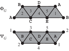
Figure 23: A relation $G$ describing co-authorship of travel guides. The Dowker complexes are dual triangulations of the Möbius strip, with $\mathbb{S}^{1}$ homotopy type. (Notes: Integers indicate authors, letters indicate cities via first letter abbreviations. Some vertices and edges appear twice for ease of viewing. Each maximal simplex is labeled with its generating author or city.)

Suppose in casual conversation a person mentions that he/she worked on producing a travel guide for Berlin. In the context of relation $G$, that information means the author is one of $\{{\tt Alice},{\tt Ben},{\tt Claire}\}$. If the author further mentions working on the travel guide for Dublin, then that identifies the author uniquely as Claire. Equivalently, the listener can infer that the author also helped write the travel guide for Caen. (This form of inference was a source of privacy problems for the Netflix Prize [17].)

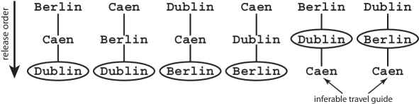
Figure 24: This figure shows the six possible sequential ways in which author #3 (Claire) of Figure 23 can mention the cities for which she co-authored travel guides. The point at which her identity becomes known in any such release sequence is circled. If Claire does not mention Caen, one can infer, via relation $G$ of Figure 23, that she co-authored a travel guide for that city as soon as she mentions the other two cities, Berlin and Dublin, in either order.

Claire was a co-author on three travel guides, for Berlin, Caen, and Dublin. Now consider the different possible sequential ways in which Claire might reveal which books she helped co-author, along with the points at which her identity becomes known (see Figure 24).

Of the six possible ways, four do not uniquely identify Claire until she has revealed all three books that she co-authored. However, two of the possible six release sequences do allow a listener to identify the author and infer an additional book that she co-authored.

This example shows how inference may be a dynamic process. While a consumer of data may wish to identify Claire with as little information as possible, the author herself may wish to delay that identification for as long as possible (perhaps for reasons of public mystery in selling books). In the example, the minimal length of an identifying attribute release sequence is two, while the maximal length is three. If Claire can control how information is released, then she can choose to reveal what might otherwise be inferred, namely that she co-authored a travel guide to Caen, thereby delaying her identification.

Finally, we observe that the order of attributes released may or may not matter. In the travel guide example, Claire should mention Caen before the end of her disclosures (if she wants to delay her identification), but the order of cities mentioned is otherwise irrelevant. The topology of the doubly-labeled poset $P_{G}$ encodes this order (in)dependence, as we will see shortly. Indeed, much of the remainder of this report examines the connection between the topology of a relation’s doubly-labeled poset and the length of attribute release sequences.

10.2 Inferences on a Lattice

The doubly-labeled poset of a relation produces a lattice [25], as follows:

Definition 13 (Galois Lattice).

Let $R$ be a relation on ${X}\mskip-1.8mu\times{Y}$, with both $\hbox{\hskip 1.0pt}{}X\!$ and $\hbox{\hskip 1.0pt}{}Y\!$ nonempty.  Let $P_{R}$ be the associated doubly-labeled poset.

(Recall from Definition 3 on page 3 that an element of $P_{R}$ is an ordered pair $(\sigma,\gamma)$, with
            $\emptyset\neq\sigma=\psi_{R}(\gamma)\in\Psi_{R}$ and  $\emptyset\neq\gamma=\phi_{R}(\sigma)\in\Phi_{R}$.

We previously defined a partial order on $P_{R}$ by $(\sigma_{1},\gamma_{1})\leq(\sigma_{2},\gamma_{2})$ iff $\sigma_{1}\subseteq\sigma_{2}$ (iff $\gamma_{1}\supseteq\gamma_{2}$).)

$P_{R}$ may already contain a unique bottom element of the form $(\sigma,Y)$, with $\sigma$ those individuals in $X\!$ who have all the attributes in $Y$. If not, we adjoin $(\hskip 0.72229pt\emptyset,Y)$ to the bottom of $P_{R}$.

$P_{R}$ may already contain a unique top element of the form $(X,\gamma)$, with $\gamma$ those attributes in $Y\!$ that every individual in $X\!$ has. If not, we adjoin $(X,\emptyset)$ to the top of $P_{R}$.

We refer to the resulting poset as the Galois lattice $P^{+}_{R}$. It has lattice operations $\vee$ and $\wedge$:

$$(\sigma_{1},\gamma_{1})\;\vee\;(\sigma_{2},\gamma_{2}) \;=\; \big{(}(\psi_{R}\circ\phi_{R})(\sigma_{1}\cup\sigma_{2}),\;\;\gamma_{1}\cap\gamma_{2}\big{)},$$

$$(\sigma_{1},\gamma_{1})\;\wedge\;(\sigma_{2},\gamma_{2}) \;=\; \big{(}\sigma_{1}\cap\sigma_{2},\;\;(\phi_{R}\circ\psi_{R})(\gamma_{1}\cup\gamma_{2})\big{)}.$$

We sometimes refer to the bottom element of $P^{+}_{R}$ by $\hat{0}_{R}$ and to the top element by $\hat{1}_{R}$.

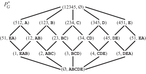
Figure 25: The lattice $P^{+}_{G}$ for the travel guide relation of Figure 23. Each element is an ordered pair of sets $(\sigma,\gamma)$ such that $\sigma=\psi_{G}(\gamma)$ and $\gamma=\phi_{G}(\sigma)$. (We have elided commas and braces in sets, for ease of viewing.) The lattice operations model inferences possible from observations. For instance, $(123,\hbox{\tt B})\wedge(345,\hbox{\tt D})\;=\;(3,\hbox{\tt B}\hbox{\tt C}\hbox{\tt D})$, meaning that observation of attributes B and D permits inference of additional attribute C and identification of author #3. (In Figure 23, attribute C is the travel guide for Caen and author #3 is Claire.) The lattice wraps around, with element $(51,\hbox{\tt E}\hbox{\tt A})$ duplicated for ease of viewing. If one removes the top and bottom elements, the remaining poset $P_{G}$ has $\mathbb{S}^{1}$ homotopy type, just like the Möbius strip.

Figure 25 shows the lattice $P^{+}_{G}$ for the travel guide relation of Figure 23. Observe how the lattice encodes attribute and association inferences (or lack thereof) via its lattice operations.

Special Cases:

It can happen that the lattice consists of a single element. For example, with relation $C$ as on page 5.2, $P^{+}_{C}=P_{C}=\{(X,Y)\}$. In particular, $\hat{0}_{C}=\hat{1}_{C}$.

Definition 13 ignores the situation in which $R$ is void. One possibility is to leave $P_{R}$ undefined and let $P^{+}_{R}=\emptyset$.  See page • ‣ A.4 in Appendix • ‣ A.4 for additional comments.

10.3 Preserving Attribute Privacy for Sets of Individuals

Theorem 10 on page 10 described the conditions under which an individual has full attribute privacy. For such an individual, the order in which that individual (or anyone) releases the individual’s attributes is irrelevant. Any order is fine. Only once all attributes have been released, can an observer uniquely identify the individual. Theorem 11 described a similar result for certain sets of individuals, including sets of individuals with whom a given individual is confusable after only some of his/her attributes have been released.

$\begin{array}[]{cl|ccc}\lx@intercol\hfil\raisebox{14.45377pt}{\hbox{\LARGE$C$}}\hfil\lx@intercol\vrule\lx@intercol&\rotatebox{90.0}{\hbox{{\sc Berlin}}}&\rotatebox{90.0}{\hbox{{\sc Caen}}}&\rotatebox{90.0}{\hbox{{\sc Dublin}}}\\[1.0pt] \hline\cr 1&(\hbox{{\tt Alice}})&\bullet&&\\ 2&(\hbox{{\tt Ben}})&\bullet&\bullet&\\ 4&(\hbox{{\tt David}})&&\bullet&\bullet\\ 5&(\hbox{{\tt Eric}})&&&\bullet\\ \end{array}$

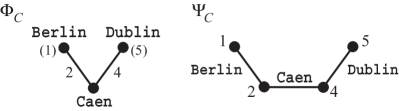
Figure 26: Relation $C$ describes $\mathop{\rm Lk}(\Psi_{G},3)$, the link of Claire in the relation of Figure 23. (Each maximal simplex in any one complex is labeled with its generating attribute or individual from the other complex. Generators of nonmaximal simplices are indicated in parentheses.)

Consider $\mathop{\rm Lk}(\Psi_{G},3)$, modeled by relation $C$ as in Figure 26. This relation describes the authors with whom Claire has collaborated, via their co-authored books. The Dowker complexes are contractible, so by either Theorem 10 or Theorem 11, we know that some attribute inference is possible involving Claire. Lemma 12 on page 12 tells us to look for a proper subset of $\{\hbox{{\sc Berlin}},\hbox{{\sc Caen}},\hbox{{\sc Dublin}}\}$ that is not  a simplex of $\Phi_{C}$. As is apparent from Figure 26, the set $\{\hbox{{\sc Berlin}},\hbox{{\sc Dublin}}\}$ satisfies these conditions, consistent with our earlier observations. Alternatively, looking at $P^{+}_{C}$ in Figure 27, we see that $(12,\hbox{\tt B})\wedge(45,\hbox{\tt D})\;=\;(\emptyset,\hbox{\tt B}\hbox{\tt C}\hbox{\tt D})$, allowing us to draw the same conclusion. Consequently, Claire should be sure to mention her travel guide for Caen early on, not leave it for last, if she wants to delay identification.

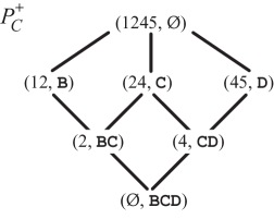
Figure 27: The lattice $P^{+}_{C}$ for the link of Claire, as given in Figure 26. (Here authors appear as integers and city names appear as first letter abbreviations.) Observe that $P^{+}_{C}$ may be viewed as a sublattice of $P^{+}_{G}$, consisting of all elements that include individual #3 there, but with that individual removed here. (See Figure 25 for $P^{+}_{G}$.)

Now let us take this reasoning one step further. Consider an element of $P^{+}_{G}$ corresponding to some state just prior to identification of Claire, for instance $(23,\hbox{\tt B}\hbox{\tt C})$. This element corresponds to both of the first two release sequences of Figure 24: Claire has mentioned her work regarding the travel guides for Berlin and Caen, but has not yet mentioned Dublin. Thus there is still some ambiguity as to her identity (it is either author #2 or author #3). In terms of Theorem 11 on page 11, $\sigma=\{2,3\}$, $\gamma=\{\hbox{{\sc Berlin}},\hbox{{\sc Caen}}\}$, and $k=2$.

$\begin{array}[]{cl|cc}\lx@intercol\hfil\raisebox{14.45377pt}{\hbox{\LARGE$Q$}}\hfil\lx@intercol\vrule\lx@intercol&\rotatebox{90.0}{\hbox{{\sc Berlin}}}&\rotatebox{90.0}{\hbox{{\sc Caen}}}\\[1.0pt] \hline\cr 1&(\hbox{{\tt Alice}})&\bullet&\\ 4&(\hbox{{\tt David}})&&\bullet\\ \end{array}$

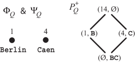
Figure 28: Relation $Q$ describes $\mathop{\rm Lk}(\Psi_{G},\{2,3\})$, the combined link of authors #2 and #3 (Ben and Claire) in the relation of Figure 23. These two authors have together collaborated with each of authors #1 and #4 (Alice and David) but have not both together collaborated with author #5 (Eric). The two Dowker complexes are each instances of $\mathbb{S}^{\kern 0.56001pt{0}}$, so essentially the same. The corresponding lattice $P^{+}_{Q}$ is also very simple.

Figure 28 shows the relation describing $\mathop{\rm Lk}(\Psi_{G},\{2,3\})$. The Dowker complexes have $\mathbb{S}^{\kern 0.56001pt{0}}$ homotopy type, thus satisfying the topological conditions of Theorem 11. Consequently, there is no attribute inference possible in the encompassing relation $G$ based on attributes that appear in the link relation $Q$. That means the order in which Claire releases the two attributes Berlin and Caen is immaterial. This conclusion is consistent with the conclusion one draws upon explicitly enumerating all release sequences, as in Figure 24.

10.4 Informative Attribute Release Sequences

This subsection defines more precisely the idea of controlled information release. These definitions will help us better understand topological holes in a relation’s Dowker complexes. Subsequently, Section 11 will explore these insights with data from the world wide web.

Definition 14 (Attribute Release Sequence).

Let $R$ be a relation on ${X}\mskip-1.8mu\times{Y}$, with both $\hbox{\hskip 1.0pt}{}X\!$ and $Y\!$ nonempty.  An attribute release sequence for $R$ is a nonempty set of attributes from $Y$ released in a particular sequential order:

$$y_{1},y_{2},\ldots,y_{k},\quad\hbox{with $k\geq 1$}.$$

We say that the sequence has length $k$.

We say that an attribute release sequence is informative if

$$y_{i}\not\in(\phi_{R}\circ\psi_{R})(\{y_{1},\ldots,y_{i-1}\}),\quad\hbox{for all $1\leq i\leq k$}.$$

(Note: for $i=1$, the requirement states that $y_{1}\not\in(\phi_{R}\circ\psi_{R})(\emptyset)=\phi_{R}(X)$.)

(We sometimes use the abbreviation 'iars' to mean either 'informative attribute release sequence' or 'informative attribute release sequences'.)

Interpretation:

When $i=1$, the argument to $\phi_{R}\circ\psi_{R}$ is the empty set, so the condition requires that $y_{1}\not\in\phi_{R}(X)$. In other words, $y_{1}$ may not be any attribute that is shared by all individuals in $X$. Any such attribute could be inferred “for free” in the context of relation $R$, and thus would not be informative. Thereafter, the condition requires that any attribute to be released not be inferable from those already released.

We are interested in understanding the extent to which order of release matters:

Definition 15 (Isotropy).

Let $R$ be a relation on ${X}\mskip-1.8mu\times{Y}$, with both $\hbox{\hskip 1.0pt}{}X\!$ and $\hbox{\hskip 1.0pt}{}Y\!$ nonempty.

Suppose $\emptyset\neq\gamma\subseteq Y$.

We say that $\gamma\!$ is isotropic if every possible ordering of all the elements in $\gamma$ forms an informative attribute release sequence for $R$.

We are interested in the minimal and maximal lengths of informative attribute release sequences:

Definition 16 (Identification and Minimal Identification).

Let $R$ be a relation on ${X}\mskip-1.8mu\times{Y}$, with both $\hbox{\hskip 1.0pt}{}X\!$ and $\hbox{\hskip 1.0pt}{}Y\!$ nonempty.

We say that a set of attributes $\gamma\subseteq Y$ identifies a set of individuals $\sigma\subseteq X$ in $R$ when $\psi_{R}(\gamma)=\sigma$.  (We sometimes alternatively say that $\gamma$ localizes to $\sigma$ in $R$.)

We say that $\gamma$ is minimally identifying (for $\sigma$) if both the following conditions hold:

1. $\psi_{R}(\gamma)=\sigma$.

2. $\psi_{R}(\gamma^{\prime})\supsetneq\sigma$ for every $\gamma^{\prime}\subsetneq\gamma$.

Definition 17 (Identification Lengths).

Let $R$ be a relation on ${X}\mskip-1.8mu\times{Y}$, with both $\hbox{\hskip 1.0pt}{}X\!$ and $\hbox{\hskip 1.0pt}{}Y$ nonempty.  Suppose $(\sigma,\gamma)\in P_{R}$.  Define the fast and slow attribute release lengths for $\sigma$ as:

$\mathop{{\rm r}_{\rm fast}}(\sigma)=\min{{\big{\{}\,\lvert\chi\rvert\;\Big{|}\;\hbox{$\chi\subseteq\gamma$ and $\psi_{R}(\chi)=\sigma$}\big{\}}}}$.

$\mathop{{\rm r}_{\rm slow}}(\sigma)=\max{{\big{\{}\,k\;\Big{|}\;\hbox{$y_{1},\ldots,y_{k}$ is an iars for $R$ and $\psi_{R}\big{(}\{y_{1},\ldots,y_{k}\}\big{)}=\sigma$}\big{\}}}}$.

An argument similar to that in Appendix D shows that the following problem is $N\!P$-complete:  Given $R$, $\sigma$, and $k$, is there some minimally identifying $\gamma$ for $\sigma$ with $\lvert\gamma\rvert\leq k$?

10.5 Isotropy, Minimal Identification, and Spheres

There is no requirement in Definition 14 that an informative attribute release sequence be a simplex in $\Phi_{R}$. (Indeed, when working with links of individuals, it can be useful to create informative attribute release sequences that are not simplices in the link, thereby identifying the given individuals in the encompassing relation, as per Lemma 12 on page 12.) However, it is always the case that any inconsistency arises only with the last attribute released:

Lemma 18 (Almost a Simplex).

Let $R$ be a relation on ${X}\mskip-1.8mu\times{Y}$, with both $\hbox{\hskip 1.0pt}{}X\!$ and $\hbox{\hskip 1.0pt}{}Y\!$ nonempty.

Suppose $\{y_{1},\ldots,y_{k}\}$ is an informative attribute release sequence for $R$.

Then $\{y_{1},\ldots,y_{k-1}\}\in\Phi_{R}$.

Proof.

If $\{y_{1},\ldots,y_{k-1}\}\not\in\Phi_{R}$, then $(\phi_{R}\circ\psi_{R})(\{y_{1},\ldots,y_{k-1}\})=\phi_{R}(\emptyset)=Y$. Since $y_{k}\in Y$, this contradicts the requirement of Definition 14. ∎

Consequently, a nonempty set of attributes $\gamma\subseteq Y$, with $\gamma\not\in\Phi_{R}$, is isotropic if and only if it is a minimal nonface of $\Phi_{R}$.  We can view such an isotropic $\gamma$ as minimally identifying for $\emptyset$.

When a nonempty set of attributes $\gamma$ is  a simplex in $\Phi_{R}$, then being isotropic is again equivalent to being minimally identifying, now for some nonempty set of individuals $\sigma$.  Moreover, topologically, we can again characterize this isotropy as a sphere, appearing via a restricted link:

Definition 19 (Restricted Link).

Let $R$ be a relation on ${X}\mskip-1.8mu\times{Y}$, with both $\hbox{\hskip 1.0pt}{}X\!$ and $\hbox{\hskip 1.0pt}{}Y\!$ nonempty.

Suppose $\sigma\in\Psi_{R}$ and $\gamma\subseteq\phi_{R}(\sigma)$.

Define relation $Q(\sigma,\gamma)$ as follows:

$$Q(\sigma,\gamma)\;=\;R\,|_{\overline{X}\times\gamma},\quad\hbox{with}\quad\overline{X}=\bigcup_{y\in\gamma}X_{y}\setminus\sigma.$$

The Dowker complexes are defined in the standard way, except for these special cases:

If $\sigma=X$, we let $\Psi_{Q(\sigma,\gamma)}$ and $\Phi_{Q(\sigma,\gamma)}$ be instances of the void complex $\emptyset$.

If $\sigma\neq X$ but $\overline{X}=\emptyset$, we let $\Psi_{Q(\sigma,\gamma)}$ and $\Phi_{Q(\sigma,\gamma)}$ be instances of the empty complex $\{\emptyset\}$.

We say that $Q(\sigma,\gamma)$ models the link of $\sigma$ restricted to $\gamma$.

$\begin{array}[]{cl|cc}\lx@intercol\hfil\raisebox{14.45377pt}{\hbox{\LARGE$Q^{\prime}$}}\hfil\lx@intercol\vrule\lx@intercol&\rotatebox{90.0}{\hbox{{\sc Berlin}}}&\rotatebox{90.0}{\hbox{{\sc Dublin}}}\\[1.0pt] \hline\cr 1&(\hbox{{\tt Alice}})&\bullet&\\ 2&(\hbox{{\tt Ben}})&\bullet&\\ 4&(\hbox{{\tt David}})&&\bullet\\ 5&(\hbox{{\tt Eric}})&&\bullet\\ \end{array}$

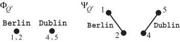
Figure 29: Relation $Q^{\prime}=Q(\sigma,\gamma)$, for the book authorship example of Figure 23, with $\sigma=\{3\}$ and $\gamma=\{\hbox{{\sc Berlin}},\hbox{{\sc Dublin}}\}$. Relation $Q^{\prime}$ describes the link of author #3 (Claire) restricted to the attribute set $\{\hbox{{\sc Berlin}},\hbox{{\sc Dublin}}\}$. See Figure 26 for the whole link relation. (Each maximal simplex in the Dowker complexes is again labeled with its generating individuals or attribute.)

Comments:

Although the previous definition looks similar to that for $\mathop{\rm Lk}(\Psi_{R},\sigma)$ on page 8, there are some differences: (a) Here, we require that $\sigma$ be a simplex in $\Psi_{R}$. (b) Here, we do not  assume $\gamma=\phi_{R}(\sigma)$, merely $\gamma\subseteq\phi_{R}(\sigma)$. (c) When $\sigma=X\in\Psi_{R}$, the current definition creates void complexes, whereas Definition 8 on page 8 creates empty complexes. (d) Finally, when $\sigma\neq{X}$ but $\gamma=\emptyset$, the current definition creates empty complexes rather than void complexes.
Interpretation: When $\sigma\in\Psi_{R}$ and $\sigma\neq{X}$, $\,Q(\sigma,\gamma)$ models those simplices of $\mathop{\rm Lk}(\Psi_{R},\sigma)$ that are witnessed by attributes in $\gamma$, plus the empty simplex.

Theorem 20 (Isotropy = Minimal Identification = Sphere).

Let $R$ be a relation and suppose $\emptyset\neq\gamma\in\Phi_{R}$.  Let $\sigma=\psi_{R}(\gamma)$. Then the following four conditions are equivalent:

1. $\gamma$ is isotropic.

2. $\gamma$ is minimally identifying (for $\sigma$).

3. $\Psi_{Q(\sigma,\gamma)}\;\simeq\;\mathbb{S}^{\kern 0.56001pt{k-2}}$, with $k=\lvert\gamma\rvert$.

4. $\Phi_{Q(\sigma,\gamma)}\;=\;\partial(\gamma)$.

See Appendix F.3 for a proof.

Collaboration Example Revisited:

To illustrate Theorem 20, consider again the example of Figure 23. Recall that together the travel guides for Berlin and Dublin identify Claire. Indeed, $\{\hbox{{\sc Berlin}},\hbox{{\sc Dublin}}\}$ is a minimally identifying set of books for Claire. It is isotropic, as Figure 24 shows. Figure 29 depicts the link of Claire restricted to $\{\hbox{{\sc Berlin}},\hbox{{\sc Dublin}}\}$, modeled by relation $Q^{\prime}$. Observe that $\Phi_{Q^{\prime}}=\partial(\{\hbox{{\sc Berlin}},\hbox{{\sc Dublin}}\})$ and that $\Psi_{Q^{\prime}}\simeq\mathbb{S}^{\kern 0.56001pt{0}}$, as the theorem asserts.

10.6 Poset Lengths and Information Release

We have seen how minimal identification appears topologically via spheres. Spheres are isotropic so perhaps it is not surprising that they encode isotropic attribute release sequences. We cannot therefore expect a spherical characterization for the problem of finding a maximally long informative attribute release sequence. Instead, we find an answer in the combinatorial structure of the doubly-labeled poset $P_{R}$ and its lattice $P^{+}_{R}$. We summarize the key results below. For proofs, see Appendix F.

Lemma 21 (Informative Attributes from Maximal Chains).

Let $R$ be a relation on ${X}\mskip-1.8mu\times{Y}$, with both $\hbox{\hskip 1.0pt}{}X\!$ and $\hbox{\hskip 1.0pt}{}Y\!$ nonempty. Suppose $\{(\sigma_{k},\gamma_{k})<\cdots<(\sigma_{1},\gamma_{1})<(\sigma_{0},\gamma_{0})\}$, with $k\geq 1$, is a maximal chain in $P^{+}_{R}$.

Define $y_{1},\ldots,y_{k}$ by selecting some $y_{i}\in\gamma_{i}\setminus\gamma_{i-1}$, for each $i=1,\ldots,k$.

Then $y_{1},\ldots,y_{k}$ is an informative attribute release sequence for $R$.

Moreover, $(\phi_{R}\circ\psi_{R})(\{y_{1},\ldots,y_{i}\})=\gamma_{i}$, for each $i=0,1,\ldots,k$.

(Notes:  (a) For a maximal chain in $P^{+}_{R}$, $\gamma_{k}=Y$ and $\sigma_{0}=X$.  (b) The hypothesis $k\geq 1$ excludes any relation $R$ for which $\hat{0}_{R}=\hat{1}_{R}$.)

Lemma 21 implies that every nontrivial maximal chain in the doubly-labeled poset associated with a relation gives rise to an informative attribute release sequence that tracks the chain.  A partial converse holds as well:

Lemma 22 (Chains from Informative Attributes).

Let $R$ be a relation on ${X}\mskip-1.8mu\times{Y}$, with both $\hbox{\hskip 1.0pt}{}X$ and $\hbox{\hskip 1.0pt}{}Y\!$ nonempty. Suppose $y_{1},\ldots,y_{k}$ is an informative attribute release sequence for $R$, with $k\geq 1$.

Let $\gamma_{i}=(\phi_{R}\circ\psi_{R})(\{y_{1},\ldots,y_{i}\})$ and $\sigma_{i}=\psi_{R}(\gamma_{i})$, for $i=1,\ldots,k$.

Then $\{(\sigma_{k},\gamma_{k})<\cdots<(\sigma_{1},\gamma_{1})<(X,\gamma_{0})\}$ is a (not necessarily maximal) chain in $P^{+}_{R}$, with $\gamma_{0}=\phi_{R}(X)$.

Consequently, one can obtain all informative attribute release sequences as subsequences of those constructed from maximal chains in $P^{+}_{R}$.

Comment about “length”:

The length $\ell(P)$ of a poset $P$ is defined to be one less than the number of elements comprising a longest chain in the poset [22]. The length of an informative attribute release sequence $y_{1},\ldots,y_{k}$ is $k$. These definitions match much like the dimension of a simplex is one less than the number of its elements.  Consequently, one obtains:

Corollary 23 (Maximal Length).

The maximum length of an informative attribute release sequence for a nonvoid relation $R$ is $\ell(P^{+}_{R})$.  (If $R$ has no iars, then the maximum length is $0$.)

Corollary 24 (Maximal Identification Length).

Suppose $R$ is a relation such that no attribute is shared by all individuals. For any $(\sigma,\gamma)\in P_{R}$, $\mathop{{\rm r}_{\rm slow}}(\sigma)=\ell(P_{Q(\sigma,\gamma)})+2$.

Collaboration Example Re-Revisited:

Returning again to the travel guide example, observe in Figure 25 that $\ell(P^{+}_{G})=4$. This tells us, by Corollary 23, that a longest informative attribute release sequence for relation $G$ contains four attributes. Indeed, we can pick three attributes to identify an individual, and then a fourth to form an inconsistency. How do we know that we can choose three attributes informatively to identify an individual? See, for example, $\mathop{\rm Lk}(\Psi_{R},\hbox{{\tt Claire}})$ in Figure 26, with associated lattice $P^{+}_{C}$ in Figure 27. In this case, $\ell(P_{C})+2=\ell(P^{+}_{C})=3$. Moreover, by the construction of Lemma 21, one can read off four different such informative sequences, namely the first four sequences appearing in Figure 24.

We thus see that $\mathop{{\rm r}_{\rm slow}}(\{\hbox{{\tt Claire}}\})=3$, and as we have seen previously, $\mathop{{\rm r}_{\rm fast}}(\{\hbox{{\tt Claire}}\})=2$. In other words, if Claire has control over how to release information, she can draw out identification for three books, while the fastest anyone can identify her is via two books.

$\begin{array}[]{c|cccc}\hbox{\large$T$}&{\tt a}&{\tt b}&{\tt c}&{\tt d}\\[2.0pt] \hline\cr 1&\bullet&\bullet&\bullet&\\ 2&&\bullet&\bullet&\bullet\\ 3&\bullet&&\bullet&\bullet\\ 4&\bullet&\bullet&&\bullet\\ \end{array}$

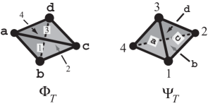
Figure 30: Relation $T$ describes four individuals with four attributes, with Dowker complexes that are boundary complexes of tetrahedra, meaning they have homotopy type $\mathbb{S}^{2}$.

In contrast, consider the tetrahedral relation of Figure 30. The Dowker complexes are boundary complexes, so we know that no attribute or association inference is possible. This is evident from the lattice $P^{+}_{T}$ depicted in Figure 31 as well. It has length 4, just as did the travel guide lattice, but the inference structure is now different. For any $(\sigma,\gamma)\in P_{T}$, with $Q=Q(\sigma,\gamma)$ modeling $\mathop{\rm Lk}(\Psi_{T},\sigma)$ on attributes $\gamma$, we see that $\Phi_{Q}=\partial(\gamma)$ and thus that $\ell(P^{+}_{Q})=\ell(P_{Q})+2=\lvert\gamma\rvert$. This tells us, by Theorem 20 and Corollary 24, that $\mathop{{\rm r}_{\rm fast}}(\sigma)=\mathop{{\rm r}_{\rm slow}}(\sigma)=\lvert\gamma\rvert$, as one would expect in an inference-free world. For a specific instance, Figure 32 depicts $Q=Q(\{3\},\{{\tt a},{\tt c},{\tt d}\})$ along with $Q$’s Dowker complexes and the lattice $P^{+}_{Q}$.

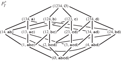
Figure 31: The lattice $P^{+}_{T}$ for the tetrahedral relation of Figure 30. Each element is an ordered pair of sets $(\sigma,\gamma)$ such that $\sigma=\psi_{T}(\gamma)$ and $\gamma=\phi_{T}(\sigma)$. (We have elided commas and braces in sets, for ease of viewing.) This lattice is isomorphic to the Boolean lattice on four atoms, consistent with the fact that $T$ preserves both attribute and association privacy. If one removes the top and bottom elements, the remaining poset $P_{T}$ has $\mathbb{S}^{2}$ homotopy type.

10.7 Hidden Holes

We saw via Theorem 20 that whenever a nonempty set of attributes $\gamma$ minimally identifies some set of individuals $\sigma$, then the link of $\sigma$, restricted to those simplices that are witnessed by attributes in $\gamma$, defines a sphere in both Dowker complexes. It is a topological hole.

All sets of individuals that are identifiable in some way, in other words, that appear in the doubly-labeled poset $P_{R}$ of a relation, must be minimally identifiable in some way. That suggests there must be holes everywhere in a relation’s Dowker complexes, and yet we do not see many holes. What is going on?

The answer is that the restricted link construction $Q(\sigma,\gamma)$ focuses on a particular subrelation, thereby exposing/highlighting a potential hole. The hole could in fact be hidden, that is, filled-in by the encompassing relation. For instance, we saw that relation $Q$ of Figure 32 defines an $\mathbb{S}^{1}$ hole. If $Q$ happened to be a subrelation of relation $R$ as in Figure 33, then $Q$ would not appear as a hole when viewed in $R$, merely a boundary.

Notice that the lattice $P^{+}_{R}$ is isomorphic to the lattice $P^{+}_{Q}$. The difference is that for every lattice element $(\sigma,\gamma)$, the set of individuals $\sigma$ includes $3$ in $P^{+}_{R}$ but not in $P^{+}_{Q}$. Consequently, the bottom element $(3,{\tt a}{\tt c}{\tt d})$ of $P^{+}_{R}$ is actually an element of the poset $P_{R}$, meaning $\Delta(P_{R})$ is a cone, hence contractible. In contrast, the poset $P_{Q}$ does not contain the bottom element $(\emptyset,{\tt a}{\tt c}{\tt d})$ of $P^{+}_{Q}$ and so $\Delta(P_{Q})$ has $\mathbb{S}^{1}$ homotopy type.

Aside:

Why not always focus on a relation’s lattice rather than its doubly-labeled poset? Because the lattice is always contractible. Any informative topology lies in the poset. See [22].

Conclusion:

Even though $R$ is contractible, it offers the same choices for informative attribute release sequences as does $Q$. More generally, the analysis of this subsection suggests that one look for potential holes in subrelations  of a given relation. Looking at links is one way to focus on subrelations. Removing individuals or attributes that represent cone apexes is another, as we just saw. More generally, any simplicial cycle may define a useful hole even though the hole appears to be filled-in. So long as one can remove any coboundary of that cycle, by restricting the relation to a subrelation without destroying the cycle, the cycle is informational. In particular, it offers opportunities for informative attribute release sequences, as the next subsection makes precise.

$\begin{array}[]{c|ccc}\hbox{\large$Q$}&{\tt a}&{\tt c}&{\tt d}\\[2.0pt] \hline\cr 1&\bullet&\bullet&\\ 2&&\bullet&\bullet\\ 4&\bullet&&\bullet\\ \end{array}$

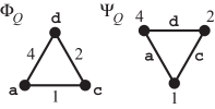
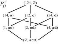
Figure 32: Relation $Q$ models $\mathop{\rm Lk}(\Psi_{T},3)$, with $T$ as in Figure 30.

$\begin{array}[]{c|ccc}\hbox{\large$R$}&{\tt a}&{\tt c}&{\tt d}\\[2.0pt] \hline\cr 1&\bullet&\bullet&\\ 2&&\bullet&\bullet\\ 3&\bullet&\bullet&\bullet\\ 4&\bullet&&\bullet\\ \end{array}$

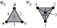
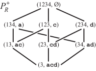
Figure 33: Relation $R$ fills in the hole of relation $Q$ from Figure 32. It is still true that $Q$ models a link, namely $\mathop{\rm Lk}(\Psi_{R},3)$. Relations $R$ and $Q$ have the same lattice structure, but the bottom element of $P^{+}_{R}$ defines the set of individuals $\{3\}$, whereas the bottom element of $P^{+}_{Q}$ defines the empty set. Thus relation $R\hbox{\hskip 1.0pt}$ defines a contractible poset for $P_{R}$, whereas relation $Q$ defines an $\mathbb{S}^{1}$ hole for $P_{Q}$.

10.8 Bubbles are Lower Bounds for Privacy

We have seen minimal identifiability characterized by holes, via Theorem 20. The previous subsections make clear that the topological characterization of $\mathop{{\rm r}_{\rm slow}}$ is not so direct. In this subsection we establish a sufficient condition. We will see that holes provide lower bounds for $\mathop{{\rm r}_{\rm slow}}$. We will focus on a relation and its links, but these results apply more generally to any hidden holes made visible by focusing on subrelations, as suggested in the previous subsection.

The connection between a relation’s poset $P_{R}$ and its lattice $P^{+}_{R}$ suggests the following:

Definition 25 (Almost a Join-Based Lattice).

Let $P$ be a finite poset. We say that $P$ is  almost a join-based lattice if adjoining a new topmost element $\hat{1}$ means $P\cup\{\hat{1}\}$ is a join semi-lattice.

Comments:

(a) We adjoin a new $\hat{1}$ even if $P$ already has a unique top (i.e., maximal) element.  (b) Since $P$ is finite, if $P$ is almost a join-based lattice, then if we adjoin both a new topmost element $\hat{1}$ and a new bottommost element $\hat{0}$, the result will be a lattice. See also [22].

This definition leads to the following result (for a proof, see Appendix G):

Theorem 26 (Many Maximal Chains).

Let $P$ be almost a join-based lattice. Suppose $P$ has reduced integral homology in dimension $k\geq 0$, that is, $\widetilde{H}_{k}(\Delta(P);\mathbb{Z})\neq 0$.

Then there are at least $(k+2)!$ maximal chains in $P$ of length at least $k$.

Interpretation:

The theorem says that a homology hole acts like a spherical hole, from the perspective of producing informative attribute release sequences. Consider again the tetrahedral relation of Figure 30. The Dowker complexes form two-dimensional spherical holes, so $k=2$ and $(k+2)!=24$. The poset $P_{T}$ is the proper part of the lattice shown in Figure 31, that is, all the elements except the topmost and bottommost. There are indeed 24 different chains of length $2$, i.e., containing three elements, in $P_{T}$.

These chains represent the 24 different ways in which one might start at a vertex of one of the Dowker complexes, walk from that vertex to the middle of an incident edge, then walk from the middle of that edge to the centroid of an encompassing triangle. For instance: the walk from the vertex $\{{\tt a}\}$ to the edge $\{{\tt a},{\tt c}\}$ to the triangle $\{{\tt a},{\tt c},{\tt d}\}$ in $\Phi_{T}$. One can think of this walk as sequential acquisition of attribute information about an individual in a particular order. The order may perhaps be determined by chance or perhaps by an individual purposefully releasing information in a particular order. Once (and only once) one has arrived at the centroid of the triangle, one has identified the individual uniquely (in this case, as individual #3).

With that observation, we finally see how the global geometry/topology of the Dowker complexes, as encoded in their doubly-labeled poset, affects inference, beyond the local simplicial collapses of the closure operators. We will presently formalize this insight via two corollaries to Theorem 26.

$\begin{array}[]{c|ccc}\hbox{\large$R$}&{\tt a}&{\tt b}&{\tt c}\\[2.0pt] \hline\cr 1&\bullet&\bullet&\bullet\\ 2&\bullet&\bullet&\bullet\\ 3&\bullet&\bullet&\bullet\\ \end{array}$

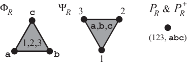
Figure 34: Relation $R$ describes three individuals all of whom have the exact same three attributes. The Dowker complexes are both triangles, but the poset $P_{R}$ is a single point. This single point captures the indistinguishability of the individuals and the attributes. In fact, $P^{+}_{R}=P_{R}$, meaning one can infer everything from nothing (in the context of relation $R$).

We caution that the dimension of a simplex in a Dowker complex is not meaningful in and of itself, since the simplex may collapse under the closure operators. (Consider the example of Figure 34, in which the Dowker complexes are fully filled-in triangles, but the doubly-labeled poset is a single point.) Instead, the length of chains in a relation’s poset is significant. Holes prevent these chains from being short, summarized as follows (proofs appear in Appendix G):

Corollary 27 (Holes Reduce Inference).

Let $R$ be a nonvoid relation. Suppose $P_{R}$ has reduced integral homology in dimension $k\geq 0$. Then there are at least $(k+2)!$ maximal chains in $P_{R}$ of length at least $k$.

Corollary 28 (Holes Defer Recognition).

Let $R$ be a nonvoid relation and let $(\sigma,\gamma)\in P_{R}$.

Define $Q=Q(\sigma,\gamma)$ as per Definition 19 and recall Definition 17, from pages 17–19.

Suppose $P_{Q}$ is well-defined and has reduced integral homology in dimension $k\geq 0$.

Then there are at least $(k+2)!$ distinct informative attribute release sequences $y_{1},\ldots,y_{\ell}$ for $R$, each with $\ell\geq k+2$, such that $\psi_{R}(\{y_{1},\ldots,y_{\ell}\})=\sigma$. Consequently, $\mathop{{\rm r}_{\rm slow}}(\sigma)\geq k+2$.

Comment:

Since $(\sigma,\gamma)\in P_{R}$ and by the assumptions about $P_{Q}$, relation $Q(\sigma,\gamma)$ models the link $\mathop{\rm Lk}(\Psi_{R},\sigma)$.

Terminology:

Here and elsewhere, the term 'distinct' means 'different' or 'distinguishable', as determined by the given context. For instance, the two sequences a, b, c  and  a, c, b  are distinct sequences even though the underlying set is $\{{\tt a},{\tt b},{\tt c}\}$ in both cases.

Collaboration Example Once Again:

The Dowker complexes for the travel guide example of Figure 23 have $\mathbb{S}^{1}$ homotopy type, meaning $P_{G}$ has homology in dimension $k=1$. Corollary 27 therefore says that there are at least 6 maximal informative attribute release sequences in $P_{G}$. Being maximal, each such sequence must identify some author, since each author is uniquely identifiable via relation $G$. In fact, we saw that there were 4 different maximal informative attribute release sequences for identifying any one author. Since there are 5 authors, $P_{G}$ actually contains at least 20 distinct maximal informative attribute release sequences. Indeed, one can readily see, via $P^{+}_{G}$ in Figure 25 on page 25, that $P_{G}$ contains exactly 20 maximal informative attribute release sequences.

Can we find these 20 sequences via our corollaries? Not by looking at individual authors, since, as we saw via Figure 26, the link of any one author is contractible, meaning that Corollary 28 does not help us directly.

There is more to be said, however: The proof of Theorem 26 actually establishes that, for certain representatives of a homology class, the maximal elements in the support of that representative each give rise to $(k+1)!$ many chains. In the collaboration example, by choosing the homology generator appropriately, this implies that for each author there are at least two informative attribute release sequences for identifying the author. That gives us 10 sequences overall for relation $G$. To find 20, we would likely want to examine links of pairs of co-authors. There are 10 such links, 5 of which look similar to the one in Figure 28 on page 28. Each of those is an instance of $\mathbb{S}^{\kern 0.56001pt{0}}$, meaning each has two different iars for identifying the pair of co-authors. That therefore gives us 10 iars for identifying certain pairs of co-authors, and thus 20 iars for identifying individual authors (each author participates in two of the identifiable pairs).

Corollary 28 further allows us to conclude that the maximal length of an informative attribute release sequence for identifying an identifiable pair of co-authors is at least two. Consequently, the maximal length of an informative attribute release sequence that identifies a given individual author must be at least (and thus exactly) three.

11 Experiments

An individual may wish to reveal information about himself/herself while delaying full identification. We saw in Section 10.8 that homology provides a lower bound on the number and length of such informative attribute release sequences. The lower bound need not be tight. In order to explore these results experimentally, we examined two datasets of different character:

Medals:

We obtained this dataset in August 2014 from

http://www.tableausoftware.com/public/community/sample-data-sets.

The dataset contained information about athletes who participated in the Olympics during the years 2000–2012.  The attribute fields that we considered were:

Age, Country, Year, Sport, Gold Medals, Silver Medals, Bronze Medals

(The last three fields counted the number of medals won by an athlete.)

Every athlete therefore had exactly 7 attributes, with each attribute taking on one of a finite discrete set of pairwise exclusive values. We represented these 7 dimensions of multivalent attributes as a collection of 223 binary attributes.

There were 8613 individuals (we regarded the same physical person in different years as distinct athletes), who partitioned into 6955 equivalence classes (for team sports, athletes often were indistinguishable).

The result was a binary relation $M$ with 6955 rows and 223 columns.

Jazz:

We assembled this relation in June 2015 by examining the website

http://www.redhotjazz.com.

The website contained information about jazz musicians and bands, mainly from the early to late-mid 20th century.

We assembled a relation $J$ whose rows were indexed by musicians and whose columns were indexed by bands, with $(m,b)\in J$ meaning that musician $m$ played in band $b$.

The result was a binary relation $J$ with 4896 rows and 990 columns.

Caution:  We were somewhat but not particularly careful in determining whether similar names constituted different spellings of the same musician’s actual name. For some bands, the website listed one or more bandmembers as “unknown”. We ignored those bandmembers. We ignored bands for whom we could not determine any bandmembers. Since our goal was to examine and compare homology and informative attribute release sequences, merely constructing a relation was sufficient for our purposes. However, it is unlikely that the resulting relation satisfied the assumption of relational completeness stated on page 3, relative to data obtainable from other sources.

We encountered the jazz website because it was the source of data for a paper on collaboration networks [12] that explored the dual nature of individuals and attributes. The paper constructed two graphs, one with musicians as vertices and bands as edges, the other with those roles reversed, then analyzed the information each representation highlighted.  We may view those graphs as the 1-skeleta of our Dowker complexes.

11.1 Compare and Contrast

We review some key differences between the two relations $M$ and $J$.

Identifiability:

The original 8613 individuals in the Olympic Medals dataset were not all uniquely identifiable. For some athletes, even knowing an athlete’s full set of 7 attributes left ambiguity as to the athlete’s identity. This was true for 2810 of the athletes. Fortuitously, an athlete’s ambiguity was fully symmetric, meaning that one could in fact partition the set of all athletes into equivalence classes. This symmetry was likely due to the fact that some competitions involved teams, with team members indistinguishable from each other. Each equivalence class then formed a uniquely identifiable “individual” in relation $M$.

For the Jazz relation, 863 of the 4896 musicians were uniquely identifiable, but 4033 were not. Unfortunately, this time the ambiguity was not fully symmetric. One could again partition the 4033 individuals into 1022 equivalence classes based on having identical rows in $J$. However, some rows remained subsets of other rows, giving a directionality to the ambiguity. For this reason, we did not pass to equivalence classes.

Attribute Size:

In the medals relation $M$, every individual had exactly 7 binary attributes, describing one value for each of the 7 possible fields:  Age, Country, Year, Sport, Gold Medals, Silver Medals, Bronze Medals. Consequently, there were also always exactly 7 binary attributes in each relation modeling the link of an athlete in $\Psi_{M}$.

In the Jazz dataset, there was no structural bound to the number of bands in which a musician might have played, so a musician’s attributes could be many. The largest number of bands in which any one musician played was in fact 44. The average was a little over 2 and the median 1. Dually, the largest band had 288 musicians, with an average of 10.4 and a median of 7.

Link Size:

For $M$, the number of other athletes in any given athlete’s link was always close to the entire set of possible athletes. With only 7 attribute fields and few distinct values, any two athletes shared almost certainly some attribute value (for instance, winning zero gold medals).

In contrast, for the 767 musicians in $J$ for whom we computed links (described further in Section 11.4), the number of other musicians in any given musician’s link was relatively small. The average was 55.3, the median 37, with a maximum of 301. With musicians generally playing in few bands, each collaborated artistically on average with only a few score fellow musicians of the 4895 musicians in the database.

11.2 Homology Computations

For each of the link relations discussed below, we computed homology of the Dowker complex $\Phi_{Q}$, with relation $Q$ modeling the link. Since our goal was to find lower bounds for informative attribute release sequences, we modified $\Phi_{Q}$ slightly, as suggested by Section 10.7. Specifically, whenever $\Phi_{Q}$ was a cone with more than one maximal simplex, we removed all its cone apexes.

Comment:  The homology lower bound results of Section 10 and Appendix G do not depend directly on the chain coefficients being integers (of course, the actual homology observed may depend on the type of coefficients). We therefore computed homology with $\mathbb{Z}_{2}$ coefficients, using the Perseus software previously written at the University of Pennsylvania. We downloaded an executable version in 2014 from http://www.sas.upenn.edu/$\sim$vnanda/perseus/.

11.3 Homology and Release Sequences in the Olympic Medals Dataset

Overall Homology:

A collection of $k$ attributes, each taking on one of a finite discrete set of pairwise exclusive values, produces Dowker complexes with homotopy types that are wedge sums of $\mathbb{S}^{\kern 0.56001pt{k-1}}$s, assuming all possible combinations of attributes are represented by individuals.

Consequently, with every individual having exactly 7 attributes, one might expect to see some homology in dimension 6. But of course, not every combination is possible. For instance, no one athlete is going to simultaneously win the gold, silver, and bronze medals in the same event. From this perspective, real-world constraints show up as absence of potential homology. In fact, relation $M$ had the Betti numbers described in Table 2, computed using $\mathbb{Z}_{2}$ coefficients:

$\begin{array}[]{c|ccccc}d&0&1&2&3&4\\[1.0pt] \hline\cr\beta_{d}&1&0&23&757&503\\ \end{array}$

Table 2: Betti numbers for the topology of the Olympic Medals relation $M$.

The table does suggest that there could be quite a few informative attribute release sequences of length at least 5 for identifying athletes ($\beta_{4}\neq 0$ in $P_{M}$ implies length 5 iars).

Link Homology:

We computed the link of each athlete in $M$ (or more precisely, of each equivalence class), and determined homology for the resulting relation, with the modifications mentioned before. Specifically, we removed all cone apexes from an athlete’s Dowker complex $\Phi_{Q}$ (assuming it contained more than one maximal simplex) before computing homology, with $Q$ being the link relation. Of the 6955 links, 3822 contained attribute cone apexes in $\Phi_{Q}$.

Table 3 summarizes the results. One may conclude more strongly now that (at least) 2198 athletes could find (at least) 120 different ways of releasing (at least) 5 of their 7 attributes without identifying themselves uniquely prior to having released all 5 attributes ($\beta_{3}\neq 0$ in $P_{Q}$ minimally implies $5!$ many iars of length 5 for relation $M$, by Corollary 28 on page 28).

$\begin{array}[]{c|ccccc}d&0&1&2&3&4\\[1.0pt] \hline\cr\hbox{\# of athletes}&229&1355&2773&2198&57\\[0.5pt] \underset{\hbox{\footnotesize{\hbox{athletes}}}}{\max}\,{\beta_{d}}&2&4&7&4&2\\ \end{array}$

Table 3: Histogram indexed by dimension $d$, describing athletes whose links $\mathop{\rm Lk}(\Psi_{M},\hbox{athlete})$ had reduced homology in dimension $d$ (after removal of attribute cone apexes from the dual complexes), for the 6955 athletes in the Olympic Medals relation $M$.  (525 of the 6955 links had no reduced homology; they do not appear in the histogram.)  Also shown are the maximum Betti numbers seen in each dimension, with the maximum taken over all possible athletes.

Informative Attribute Release Sequences:

We computed a maximal length informative attribute release sequence for each link relation. One can find such a sequence by searching for a least-cost path from $\hat{1}_{Q}$ to $\hat{0}_{Q}$ in $P^{+}_{Q}$, picking attributes along the way as per the construction of Lemma 21 on page 21, with cost being the number of attributes inferred as one traverses the path. Here $Q$ is again the link relation. Of the 6955 athletes, 6229 actually had a maximal informative attribute release sequence of length 7. Each such athlete could order his/her attributes in such a way that his/her identity would not become fully known until s/he had released all 7 attributes. Of the remaining athletes, 719 had a maximal informative attribute release sequence of length 6, and 7 had a maximal length of 5.

Of course, Corollary 28 on page 28 makes a stronger claim, suggesting possible permutability of some attributes. Consequently, we computed for each link relation all possible isotropic sets of attributes (see again Definition 15 on page 14, now with $Q$ in place of $R$). Table 4 summarizes the results:

$\begin{array}[]{c|ccccc}\lvert\kappa\rvert&2&3&4&5&6\\[2.0pt] \hline\cr\hbox{\# of athletes}&6955&6955&6955&5568&171\\[1.0pt] \underset{\hbox{\footnotesize{\hbox{athletes}}}}{\max}\,{\lvert\{\kappa\}\rvert}&21&35&35&21&5\\ \end{array}$

Table 4: Histogram indexed by size $\lvert\kappa\rvert$, describing athletes whose link relations contained isotropic attribute sets $\kappa$. An athlete could have several distinct (possibly overlapping) such sets for any given size. Also shown therefore are the maximum numbers of such sets, with the maximum taken over all possible athletes. For example: 171 athletes had at least one isotropic set of size $6$, and the maximum number of isotropic sets of size $6$ any one athlete had was 5.

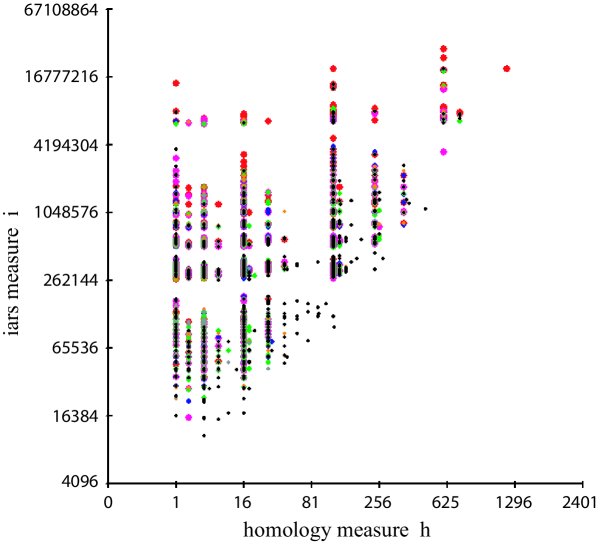
Figure 35: Scatterplot describing each athlete’s link in the medals relation $M$. The scatterplot shows for each link a point $(h,i)$, with $h$ a measure of the link’s homology (after removal of attribute cone apexes) and $i$ a measure of how many significant informative attribute release sequences exist for the link relation. The scatterplot suggests that the homology measure $h$ serves as a loose lower bound for the iars measure $i$.  See also Corollary 28 on page 28.
(The colors and radii indicate the numbers of athletes in the links.  The color ordering and size boundaries are:
            black–₆₈₂₁–silver–₆₈₃₁–orange–₆₈₅₁–green–₆₈₅₉–blue–₆₈₆₅–magenta–₆₈₇₂–red.
In this figure, the boundaries between colors were chosen so that each bucket would hold roughly 1000 links. As one can see, the number of athletes in a link was generally large.)

Scatterplot:

Finally, we computed for each link a pair of numbers $(h,i)$, with $h$ representing a measure of link homology and $i$ representing a measure of informative attribute release sequences for the link relation. The resulting scatterplot appears in Figure 35.

The exact formulas for $h$ and $i$ are not that significant, but we mention them here for completeness. To obtain a measure of homology, we assembled for each link a vector with the Betti numbers computed earlier: $(\beta_{0},\beta_{1},\beta_{2},\beta_{3},\beta_{4})$. We determined maximum values for each component (as given in Table 3). We could then think of any such vector as defining, in reverse order, a varying-radix numeral. We converted that numeral to an integer. For example, a link with Betti vector $(2,3,6,0,0)$ would have $h$ value ${2+3{\cdot}(2+1)+6{\cdot}(4+1){\cdot}(2+1)}={101}$. A link relation that remains contractible after removal of attribute cone apexes would have $h$ value $1$. In order to graph the scatterplot nicely, we scaled the $h$-axis by taking a fourth root.

We computed a link’s $i$ value similarly, now from the following vector of data: $(\ell_{\rm max},c_{2},c_{3},c_{4},c_{5},c_{6})$. Here $\ell_{\rm max}$ is the largest $\ell$ in an informative attribute release sequence $y_{1},\ldots,y_{\ell}$ for the link relation, while $c_{k}$ is the number of different isotropic attribute sets $\kappa$ in the link relation such that $\lvert\kappa\rvert=k$. We scaled the $i$-axis by taking a logarithm.

11.4 Homology and Release Sequences in the Jazz Dataset

Overall Homology:

Given the large number of bands in which some musicians played, and given memory constraints of our machines, we did not compute homology for the whole Jazz relation $J$. Instead, we computed homology for restricted relations consisting of musicians who played in fewer than 20 bands. This covered 4856 of the 4896 musicians in the overall relation. Since we did not see any homology above dimension 2 after considering several of these restricted cases, we used the 4-skeleton (all simplices of dimension 4 or less) of $\Phi_{\!J}$ as proxy for the topology of the whole relation $J$ and computed its homology. Table 5 summarizes the results. Using a graph algorithm, we verified that the whole relation $J$ did indeed have 107 components, as indicated by $\beta_{0}$ for the 4-skeleton $\Phi^{(4)}_{\!J}$. Given the low dimension of homology for the restricted relations, conceivably even $J$ might not tell us much about the length of informative attribute release sequences for the various musicians, suggesting we look at links.

$\begin{array}[]{cc|c|ccccc}b&\Sigma&m&\beta_{0}&\beta_{1}&\beta_{2}&\beta_{3}&\beta_{4}\\[3.0pt] \hline\cr 14&\Phi_{\!J|b}&4819&111&613&20&0&0\\[2.0pt] 15&\Phi_{\!J|b}&4831&111&613&32&0&0\\[2.0pt] 16&\Phi_{\!J|b}&4838&111&605&42&0&0\\[2.0pt] 17&\Phi_{\!J|b}&4848&110&603&58&0&0\\[2.0pt] 18&\Phi_{\!J|b}&4851&110&603&65&0&0\\[2.0pt] 19&\Phi_{\!J|b}&4856&109&596&75&0&0\\[5.0pt] \infty&\Phi^{(4)}_{\!J}&4896&107&550&93&10&-\\[4.0pt] 15&\Phi_{\!J^{\prime}}&767&18&595&32&0&0\\ \end{array}$

Table 5: Betti numbers for subcomplexes $\Sigma$ of $\Phi_{\!J}$, with $J$ being the Jazz relation. The first six rows correspond to restrictions of $J$ to musicians who played in at most $b$ bands. For each row, $m$ indicates the number of musicians in the relation. The penultimate row describes the 4-skeleton of $\Phi_{\!J}$. The last row refers to a relation $J^{\prime}$ described further in the text.

Link Homology:

We computed the link of some of the musicians in $J$, and determined homology for the resulting relations (again after removal of attribute cone apexes, when appropriate). Table 6 summarizes the results. Given the inability to uniquely identify some musicians even knowing all their bands (as described in Section 11.1) and the difficulty of computing homology when musicians played in many bands, we computed links only for a subset of the musicians. We required each musician to be uniquely identifiable, to have played in at most 15 bands, and to have a nontrivial link. There were 767 such musicians. Betti numbers for the relation $J^{\prime}$ representing the restriction of $J$ to these 767 musicians also appear in Table 5. (Note, however, that we computed the complete link $\mathop{\rm Lk}(\Psi_{\!J},\hbox{musician})$ for each of the 767 musicians, not merely $\mathop{\rm Lk}(\Psi_{\!J^{\prime}},\hbox{musician})$.)  We removed attribute cone apexes from the link relation for 106 of these 767 musicians.

$\begin{array}[]{c|cccc}d&0&1&2&3\\[2.0pt] \hline\cr\hbox{\# of musicians}&604&145&20&1\\[1.0pt] \underset{\hbox{\footnotesize{\hbox{musicians}}}}{\max}\,{\beta_{d}}&7&6&3&1\\ \end{array}$

Table 6: Histogram indexed by dimension $d$, describing musicians whose links $\mathop{\rm Lk}(\Psi_{\!J},\hbox{musician})$ had reduced homology in dimension $d$ (after removal of attribute cone apexes from the dual complexes), for the 767 musicians who were uniquely identifiable in $J$, played in at most 15 bands, and had nontrivial link.  (52 of the 767 links had no reduced homology; they do not appear in the histogram.)  Also shown are the maximum Betti numbers seen in each dimension, with the maximum taken over the 767 possible musicians. For $d=0$, this means that 604 of the 767 musicians had collaborations with other musicians that split into pairwise disjoint groups. The maximum number of such components for any one musician was 7.

These results suggest that the relationships to other musicians do indeed not have many high-dimensional holes in them. Recall, by Corollary 28 on page 28, one can assert the existence of at least $(k+2)!$ distinct informative attribute release sequences of length at least $k+2$ for any musician with a $k$-dimensional hole. For almost all musicians this lower bound means 2 sequences of length 2, for some it means 6 sequences of length 3, for a few it means 24 sequences of length 4, and for one musician it means 120 sequences of length 5. These implications are roughly consistent with the data for informative attribute release sequences described next, though, as expected for the theoretical reasons discussed earlier, they constitute lower bounds.

Informative Attribute Release Sequences:

We computed a maximal length informative attribute release sequence for each link relation. Table 7 summarizes the results. We mention in passing: Any attribute release sequence that was informative for a musician’s link relation was also informative for the encompassing relation $J$ (by Lemma 12(ii) on page 12). For a few musicians, the maximal sequence found within the link relation $Q$ could be further extended in the encompassing relation $J$, with a prefix of one attribute, namely an attribute shared by all members of the link, yet remain informative and identifying within $J$. This occurred for the 17 musicians whose maximum sequence length $\ell$ in the musician’s link was 1.

We also computed for each link relation all possible isotropic sets of attributes. Table 8 summarizes those results.

$\begin{array}[]{c|ccccccccccc}\ell&1&2&3&4&5&6&7&8&9&10&11\\[2.0pt] \hline\cr\hbox{\# of musicians}&17&248&218&125&72&35&23&15&11&2&1\\ \end{array}$

Table 7: Histogram of musicians, indexed by length $\ell$ of a longest informative attribute release sequence for the musician’s link relation, for the 767 musicians described in the text.

$\begin{array}[]{c|cccc}\lvert\kappa\rvert&2&3&4&5\\ \hline\cr\hbox{\# of musicians}&750&219&49&3\\[1.0pt] \underset{\hbox{\footnotesize{\hbox{musicians}}}}{\max}\,{\lvert\{\kappa\}\rvert}&105&202&40&2\\ \end{array}$

Table 8: Histogram indexed by size $\lvert\kappa\rvert$, describing musicians whose link relations contained isotropic attribute sets $\kappa$. Also shown are the maximum numbers of such sets, with the maximum taken over the 767 possible musicians described in the text.

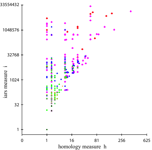
Figure 36: Scatterplot describing the links computed for 767 of the musicians in the Jazz relation $J$. The scatterplot shows for each link a point $(h,i)$, with $h$ a measure of the link’s homology (after removal of attribute cone apexes) and $i$ a measure of the link’s informative attribute release sequences.
(The colors and radii indicate the numbers of musicians in the links. Link sizes were fairly small.  The color ordering and size boundaries are:
            black–₅–silver–₁₀–orange–₂₀–green–₅₀–blue–₁₀₀–magenta–₂₀₀–red.
In this figure, the buckets could hold noticeably varying numbers of links.)

Scatterplot:

We computed for each link a pair of numbers $(h,i)$, with $h$ representing a measure of homology and $i$ representing a measure of the link’s informative attribute release sequences, much as for the medals relation $M$ of Section 11.3. Figure 36 depicts the scatterplot.

12 Inference in Sequence Lattices

We have seen how a relation gives rise to a lattice via the Galois connection, as per Definition 13 on page 13. The lattice structure describes the ways in which privacy may be preserved or lost. Consequently, when thinking about privacy, perhaps one can also start with lattices that do not necessarily arise initially from relations.

This section will look at inferences from sequences of observations. The next section examines strategy obfuscation in planning with uncertainty.

We should mention some equivalences: Lattices are particular kinds of partially ordered sets (posets). Posets and simplicial complexes are topologically identical; one can move back and forth between these representations while preserving homeomorphism type (see [22] and Appendix A). Furthermore, one may describe a finite simplicial complex by a relation in several different ways that preserve homotopy type, including ways in which one of the two resulting Dowker complexes is identical to the original simplicial complex. For instance, maximal simplices can play the role of individuals and vertices can play the role of attributes. In short, one has three different categories of structures with which to think about privacy: relations, simplicial complexes, and lattices. One may start with any one representation and build the other two from that.

12.1 Sequence Lattices for Dynamic Attribute Observations

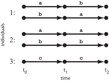
Figure 37: Three types of individuals and the attributes each might reveal in two successive time intervals.

Consider the dynamic process of Figure 37. The process models observations of individuals who reveal attributes over successive time steps. There are three possible individuals (or more generally, types of individuals). The first individual emits attributes “a” and “b” alternatingly at successive times, but one does not know which of those attributes one might see first. The second individual always emits the same attribute, either “a” or “b”, but one does not know a priori which it is. The third individual always emits the same attribute “c”.

$\begin{array}[]{c|ccc}\hbox{\Large$S$}&{\tt a}&{\tt b}&{\tt c}\\[2.0pt] \hline\cr 1&\bullet&\bullet&\\ 2&\bullet&\bullet&\\ 3&&&\bullet\\ \end{array}$

$\begin{array}[]{c|ccccc}\hbox{\Large$T$}&{\tt a}{\tt a}&{\tt b}{\tt b}&{\tt a}{\tt b}&{\tt b}{\tt a}&{\tt c}{\tt c}\\[2.0pt] \hline\cr 1&&&\bullet&\bullet&\\ 2&\bullet&\bullet&&&\\ 3&&&&&\bullet\\ \end{array}$

Figure 38: Relation $S$ describes individuals and single attributes, while $T$ describes individuals and sequences of two attributes.

A relation for these (types of) individuals that models the individuals in terms of single attributes appears as relation $S$ in Figure 38. Individual #3 is distinguishable from the other two individuals, but the relation provides no means for distinguishing those two individuals from each other. The relation is homogeneous with regard to single attributes for individuals #1 and #2. Of course, we can see from the dynamic process of Figure 37, that distinguishing information appears via sequences of two attributes. Relation $T$ of Figure 38 models such sequences. Now all three individuals are uniquely identifiable. Should one wish to model inferences based on both one and two observations, one could use the relation $S\cup T$.

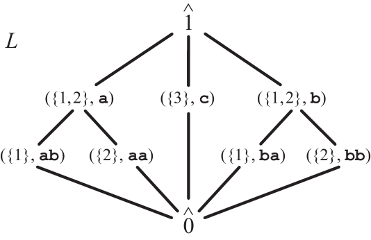
Figure 39: Lattice representing the dynamic process of Figure 37.

That jump from single to double attributes is useful, but where does it come from intrinsically? After all, without additional knowledge, we might simply consider infinitely long sequences, even though those would not add anything in this example. In fact, the dynamic process of Figure 37 gives us the information. It is itself basically a decision tree that amounts to the lattice of Figure 39. In that figure, we have annotated each internal node of the lattice with an ordered pair, consisting of a set of individuals and either a single attribute or a sequence of two attributes. This lattice differs from previous ones in this report in that a set of individuals (or attributes, more generally) is no longer constrained to appear in at most one node of the lattice. By allowing multiple nodes, we enhance our ability to encode state in the lattice. For example, observing attribute “a” carries different meaning depending on whether one has already seen attribute “a” or attribute “b” or no attribute at all. Also: While we could have included $(\{3\},{\tt c}{\tt c})$ in the lattice, we did not need that element.

In the lattice of Figure 39 it is tempting to merge the two identifying nodes for individual #1 into one node and to merge the two identifying nodes for individual #2 into one node. There is apparently no harm in doing so, in that the decision process would still be correct. However, the resulting structure would no longer be a lattice but merely a poset. That may or may not be desirable in a given application. For instance, using homology to estimate lower bounds for how long one can delay identification suggests using almost a join-based lattice, if one wishes to fulfill the hypotheses of Theorem 26 on page 26.

If we did want to merge nodes as just described, while maintaining a lattice, then we would perhaps also merge the two nodes containing the set $\{1,2\}$, giving us the lattice of Figure 40. This lattice is similar to the lattice $P^{+}_{S\cup T}$ that one would construct from the relation $S\cup T$, except that it does not include singleton attributes in the nodes identifying individuals #1 and #2 and it does not include the sequence “cc” in the node identifying individual #3.

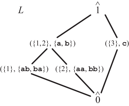
Figure 40: Modified lattice of Figure 39, after merging some nodes.

Regardless, the lattices of Figures 39 and 40 encode the inferences possible for the dynamic process of Figure 37. In particular, if we observe either attribute “a” or attribute “b”, then we know the set of possible individuals is $\{1,2\}$; we have excluded individual #3. Moreover, if we observe any two-attribute sequence, with attributes drawn from $\{{\tt a},{\tt b}\}$, then we can identify the observed individual uniquely as either #1 or #2. Thus the required sequences come directly from the dynamic process, not requiring an explicit intermediate representation as a relation. (One might argue, however, that a relation is implicit in our reasoning.)

12.2 Lattices of Stochastic Observations

The dynamic sequence perspective incorporates repeated randomized response within the lattice framework. Instead of arising via a (non)deterministic process as in Figure 37, the attributes “a” and “b” for two (types of) individuals could flow from a stochastic process. One obtains an infinite lattice determined by increasingly longer sequences of observations. Depending on the confidence intervals one wishes to set, one obtains stochastic decision regions such as those sketched in Figure 41, with a central region of ambiguity, bounded by regions of exclusion, for identifying individuals.

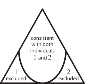
Figure 41: Sketch of an inference lattice for sequences of randomized response queries.

12.3 General Inference Lattices

Lattices are useful tools for inference. Rather than work with completely arbitrary lattices, we give here a definition that makes explicit the existence of two underlying structures over which we wish to perform inferences. However, we no longer assume a pair of underlying discrete spaces $X$ and $Y$ for individuals and attributes, but instead posit posets $P$ and $Q$. The connection to our earlier relational perspective is that $P$ would be the powerset of $X$ and $Q$ the powerset of $Y$. By allowing potentially different posets $P$ and $Q$ for a given lattice $L$, one can in some instances obtain different “views” of that lattice, thereby increasing flexibility in the interpretation process. For instance, $Q$ might consist of all sequences up to a specified length or it might consist of sets of such sequences.

Definition 29 (Inference Lattice).

Let $P$ and $Q$ be finite posets.

An inference lattice $L$ with respect to $P$ and $Q$ is a bounded lattice whose proper part $\overline{L}$ consists of ordered pairs $(p,q)$, with $p\in P$ and $q\in Q$, satisfying the following conditions:

For all $(p_{1},q_{1})$ and $(p_{2},q_{2})$ in $\overline{L}$:

1. $(p_{1},q_{1})\leq_{L}(p_{2},q_{2})$ if and only if $p_{1}\leq_{P}p_{2}$ and $q_{1}\geq_{Q}q_{2}$;

2. $(p_{1},q_{1})\vee_{L}(p_{2},q_{2})$ is either $\hat{1}_{L}$ or a pair $(p,q)\in\overline{L}$ such that $p$ is an upper bound for both $p_{1}$ and $p_{2}$ in $P$ and $q$ is a lower bound for both $q_{1}$ and $q_{2}$ in $Q$;

3. $(p_{1},q_{1})\wedge_{L}(p_{2},q_{2})$ is either $\hat{0}_{L}$ or a pair $(p,q)\in\overline{L}$ such that $p$ is a lower bound for both $p_{1}$ and $p_{2}$ in $P$ and $q$ is an upper bound for both $q_{1}$ and $q_{2}$ in $Q$.

(Note that $\,\,\hat{0}_{L}<_{L}(p,q)<_{L}\hat{1}_{L}\,$ for every $(p,q)\in\overline{L}$, when $\overline{L}\neq\emptyset$.
Also, be aware that $\overline{L}$ need not, and generally will not, contain all possible pairs $(p,q)$ of $\,{P}\mskip-0.8mu\times{Q}$.)

Inference Protocol:

Suppose we have observed some $q\in Q$.  How should we interpret that observation in terms of the lattice $L$?   Here is a possible protocol:

(In terms of our earlier relational model, one may view this protocol as inferring sets of individuals from sets of attributes.)

• Let $\Gamma={\left\{(p^{\prime},q^{\prime})\in\overline{L}\;\left|\;q\;\leq_{Q}\;q^{\prime}\right.\right\}}$.

• If $\Gamma=\emptyset$, then we view $q$ as inconsistent, producing interpretation $\hat{0}_{L}\in L$.

• Otherwise, let $\Gamma_{\rm max}$ consist of all the maximal elements of $\Gamma$ (maximal with respect to the partial order on $L$). We view $q$ as implying this set of elements in $L$. One can project each of those elements onto its $P$ coordinate, if that is useful.

There is a dual protocol for interpreting an observation $p\in P$:

(In terms of our earlier relational model, one may view this protocol as inferring sets of attributes from sets of individuals.)

• Let $\Sigma={\left\{(p^{\prime},q^{\prime})\in\overline{L}\;\left|\;p\;\leq_{P}\;p^{\prime}\right.\right\}}$.

• If $\Sigma=\emptyset$, then we view $p$ as inconsistent, producing interpretation $\hat{1}_{L}\in L$.

• Otherwise, let $\Sigma_{\rm min}$ consist of all the minimal elements of $\Sigma$ (minimal with respect to the partial order on $L$). We view $p$ as implying this set of elements in $L$. Again, one can project each of those elements onto its $Q$ coordinate, if that is useful.

Comments:

(1) In our previous relational setting, the structure of Galois lattices ensured that, for nonempty observations, each of $\Gamma_{\rm max}$ and $\Sigma_{\rm min}$ never contained more than one element. That need not be true for general inference lattices.  (2) One may augment the previous protocols, so as to regard some element(s) of $Q$ much like the empty attribute simplex, giving interpretation $\hat{1}_{L}\in L$. Similarly, some element(s) of $P$ might have interpretation $\hat{0}_{L}\in L$.

Example:

Consider Figure 42. Poset $P$ models subsets drawn from the set of two individuals $\{1,2\}$, while poset $Q$ models sequential observations of “a” and “b”, of lengths one and two, as in our earlier example of Figure 37. (For presentational simplicity, $P$ and $Q$ ignore individual #3 and attribute “c”, instead focusing on individuals $\{1,2\}$ and attributes $\{{\tt a},{\tt b}\}$.) Let lattice $L$ be as in Figure 39.  Assume the interpretation of $\emptyset\in P$ is $\hat{0}_{L}$ in $L$, and that of $\,\hat{0}\in Q$ is $\hat{1}_{L}$.

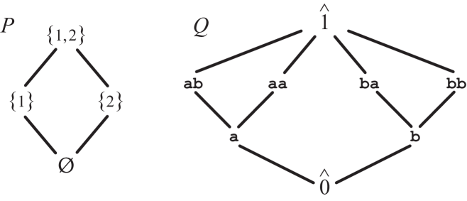
Figure 42: Poset $P$ models some sets of individuals; poset $Q$ models some sequences of attributes.

Observing an attribute:

Suppose we have observed attribute “b”, i.e., $q={\tt b}$. What can we infer from $q$ in $P$ via $L$?  Let us follow the protocol given earlier:

• The subposet of $Q$ consisting of elements $q^{\prime}$ greater than or equal to $q$ is: $$\begin{diagram}$$ .

• Consequently, $\Gamma$ is the following subposet of $L$:     $$\begin{diagram}$$ .

• There is one maximal element in $\Gamma$, so $\Gamma_{\rm max}=\{(\{1,2\},{\tt b})\}$.

Projecting onto the $P$ component tells us how to interpret $q$: The observation “b” must have come from either individual #1 or individual #2, as one would hope. (This conclusion would hold as well if $P$ had modeled individual #3 and if $Q$ had modeled attribute “c”.)

Observing an individual:

Suppose we have observed individual #1, i.e., $p=\{1\}$. What can we infer from $p$ in $Q$ via $L$?  Again, let us follow the inference protocol given earlier:

• The subposet of $P$ consisting of elements $p^{\prime}$ greater than or equal to $p$ is:     $$\begin{diagram}$$ .

• Consequently, $\Sigma$ is the following subposet of $L$:     $$\begin{diagram}$$ .

• The minimal elements of $\Sigma$ give us $\Sigma_{\rm min}=\{(\{1\},{\tt a}{\tt b}),\;(\{1\},{\tt b}{\tt a})\}$.

Projecting onto the $Q$ component tells us how to interpret $p$: The individual observed can or did reveal one of the two-attribute sequences “ab” or “ba”.

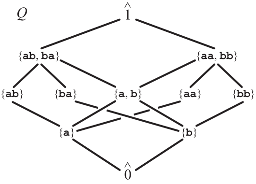
Figure 43: Poset $Q$ modeling sets of attribute sequences, for inferences in the lattice of Figure 40.

Comment:

The poset $Q$ of Figure 42 would not be relevant for inferences in the lattice of Figure 40, since that lattice now models attribute observations involving “a” and/or “b” as sets of sequences rather than merely as sequences. We would instead probably want $Q$ to be something like the poset of Figure 43. So even though $L$ has become simpler than in Figure 39, $Q$ has become more complicated. On the other hand, the new $(L,P,Q)$ triple means that one can infer $(\{1,2\},\{{\tt a},{\tt b}\})$ from the observation “b”. As before, that says the observation “b” must have come from individual #1 or #2, but it also says directly that the individual could alternatively have produced attribute “a”. In summary, by altering the triple $(L,P,Q)$, one changes the possible inferences.

Aside:

The poset $Q$ of Figure 43 is a conveniently chosen finite subposet of a particular infinite poset modeling sets of sequences. In that model, each set is required to be finite and prefix-free, meaning that if two distinct sequences appear in an element of $\overline{Q}$, neither may be a prefix of the other. The partial order on $\overline{Q}$ is defined by: $q_{1}\,\leq_{Q}\,q_{2}$ precisely when every sequence in $q_{1}$ is a prefix of (possibly equal to) some sequence in $q_{2}$.   (Notation: $\overline{Q}$ is the proper part of $Q$, that is, $\overline{Q}=Q\setminus\{\hat{0},\hat{1}\}$, and $\hat{0}<q<\hat{1}$ for every $q\in\overline{Q}$.)

13 Lattices for Strategy Obfuscation

In Section 12, we saw sublattices of powerset lattices, those being prototypical examples of Boolean lattices. A related example is given by strategy complexes [6, 7], which may be viewed as lattices of (stochastic) partial orders formed from potentially nondeterministic or stochastic transitions in a graph. The basic elements in such a lattice are strategies for attaining various goals. Our work on privacy now raises the question of strategy obfuscation: How can someone reveal the actions of a strategy in a fashion that delays identification of the strategy?

13.1 Strategies for Nondeterministic Graphs

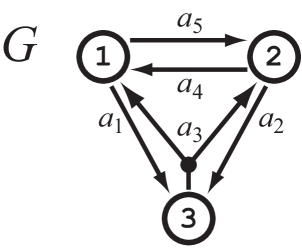
Figure 44: A graph $G$ with three states, four deterministic actions, and one nondeterministic action ($a_{3}$).

For a very simple example, consider the graph of Figure 44. We might think of this graph as modeling some kind of dynamic system, for instance, a person driving between three shopping malls or a robot moving among clutter in a warehouse or an intruder in a server network.

There are three states in the graph, along with five actions. Each action has a source  state and one or more target  states, indicated in the figure by arrows. An action may be executed  when the system is at the source state of the action, causing the system to move from the action’s source state to one of its target states.

Four of the actions, $\{a_{1},a_{2},a_{4},a_{5}\}$, are standard deterministic directed edges, leading for certain from one state to another. The remaining action, $a_{3}$, is nondeterministic. Nondeterminism of $a_{3}$ means that if the system is at state 3 and executes action $a_{3}$, then the precise outcome is uncertain: The system might move either to state 1 or to state 2. Nondeterminism is potentially adversarial: The precise target state attained is unpredictable and could vary nonstochastically on different executions of the action, perhaps determined by an adversary outside the graph. One may generalize this idea to include stochastic actions along with deterministic and nondeterministic actions, thus modeling adversarial combinations of Markov chains [6, 7].

In the nondeterministic setting, a strategy  is a set of actions whose underlying directed edge set contains no directed cycles. The semantics of a strategy are: If the system is at the source state of an action in the strategy, then the system executes that action. If the strategy contains multiple actions with that same source state, then the actual action executed is again determined nondeterministically. For instance, in the example, if actions $a_{1}$ and $a_{5}$ both appear in a strategy, then the strategy is indifferent as to whether the system will transition to state 2 or to state 3 from state 1. One or the other will occur. If a strategy does not contain any action with a given source state, then the system will stop moving if it is ever in that state.

The lattice operations for strategies are set union and set intersection, with one proviso: Suppose $\sigma_{1}$ and $\sigma_{2}$ are two strategies. Each strategy is a set of actions with no directed cycles in its underlying directed edge set. If the union of the two strategies, $\sigma_{1}\cup\mskip 1.0mu\sigma_{2}$, contains a directed cycle in its underlying directed edge set, then the lattice operation becomes $\sigma_{1}\vee\sigma_{2}=\hat{1}$, with $\hat{1}$ the top element of the lattice. That top element represents cyclicity. The bottom element $\hat{0}$ of the lattice is equivalent to the empty strategy $\emptyset$, amounting to no motion.

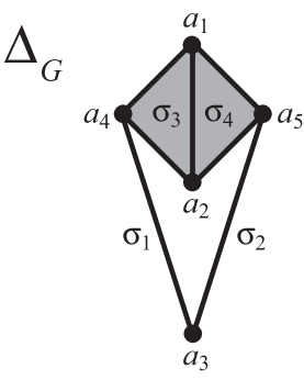
Figure 45: The strategy complex for the graph of Figure 44. Each vertex represents an action, as indicated by the labels. Each maximal simplex also has a label, for the purposes of Figure 46.

Rather than draw a lattice of strategies $L$, it is more convenient to draw an equivalent simplicial complex whose vertices are the (acyclic) actions of the graph. This simplicial complex is denoted by $\Delta_{G}$ and is called the strategy complex  of $G$. The connection is that the proper part of the lattice is the face poset of the simplicial complex, that is $L\setminus\{\hat{0},\hat{1}\}={\mathfrak{F}}(\Delta_{G})$. Figure 45 shows the strategy complex for the graph of Figure 44. The constituent simplices of the strategy complex are strategies, that is, all sets of actions whose underlying directed edge sets are acyclic.

Now that we have a simplicial complex, we can form a relation, whose “individuals” are all maximal strategies of the complex and whose “attributes” are the underlying actions, as shown in Figure 46. The figure also shows each maximal strategy’s goal, that is, the state at which the strategy would stop moving.  (In general, a strategy, even a maximal strategy, may have a multi-state goal set, but in this example the goals of all maximal strategies are singleton states.)  Of course, a system could employ nonmaximal strategies, but for identifiability purposes it is natural to consider maximal strategies.

$\begin{array}[]{c|ccccc}\hbox{\Large$A$}&a_{1}&a_{2}&a_{3}&a_{4}&a_{5}\\[2.0pt] \hline\cr\sigma_{1}&&&\bullet&\bullet&\\ \sigma_{2}&&&\bullet&&\bullet\\ \sigma_{3}&\bullet&\bullet&&\bullet&\\ \sigma_{4}&\bullet&\bullet&&&\bullet\\ \end{array}$

$\begin{array}[]{c}\hbox{Goal}\\[2.0pt] \hline\cr 1\\ 2\\ 3\\ 3\\ \end{array}$

Figure 46: Relation $A$ describes the strategy complex of Figure 45 in terms of its maximal simplices and their constituent actions. The rightmost column shows each maximal strategy’s goal, i.e., that state at which motion ceases.

We make the following observations:

• There is at least one strategy for attaining each state in the graph, meaning it is possible to move from every state to every other state, despite uncertainty in the outcome of one of the actions. Such graphs are called fully controllable in [6, 7], and have properties similar to those of strongly connected directed graphs.

• Each maximal strategy contains  two  informative attribute (i.e., action) release sequences, with each sequence consisting of two actions that together identify the strategy. For instance, for $\sigma_{1}$, one could reveal actions $a_{3}$ and $a_{4}$ in either order, identifying $\sigma_{1}$ only after revealing both actions. For $\sigma_{3}$, one could reveal actions $a_{1}$ and $a_{4}$ in either order, now identifying $\sigma_{3}$ only after revealing both actions.

• Some actions reveal the goal even though they do not identify the maximal strategy. In particular, actions $a_{1}$ and $a_{2}$ each individually reveal the goal to be 3. (The two actions are in fact equivalent in $A$, in that either one implies the other.) For instance, if one knows that $a_{1}$ is in a maximal strategy $\sigma$, then one knows that the strategy cannot also contain $a_{3}$, as adding $a_{3}$ would create a directed cycle in the underlying directed edge set. Action $a_{2}$ must therefore also be in the strategy, since the strategy is maximal. Consequently, the goal is state 3 and $\sigma$ is either $\sigma_{3}$ or $\sigma_{4}$. The difference between these two maximal strategies is a choice between $a_{4}$ and $a_{5}$. That choice does not affect the final goal, but could affect intermediate motions and the time to reach the goal. A rough analogy is knowing that a car on a freeway must continue on the freeway until at least the next exit but has a choice between lanes enroute.

• Each maximal strategy contains at least one  informative action release sequence consisting of two actions that do not reveal the goal until the second action has been released. For instance, for $\sigma_{3}$, one could first release $a_{4}$, leaving open the possibility of either state 1 or state 3 being the goal, then subsequently release either $a_{1}$ or $a_{2}$.

The rest of this section and Appendix H explore these observations more generally.

13.2 Connecting the Topologies of Strategy Complexes and Privacy

Notation:

• $G=(V,{\mathfrak{A}})$ denotes a graph with states $V\!$ and actions ${\mathfrak{A}}$. An action may be deterministic, nondeterministic, or stochastic. (For simplicity, we assume here that $V\!\neq\emptyset$ and ${\mathfrak{A}}\neq\emptyset$.)

• $\Delta_{G}$ denotes the strategy complex of $G$; it includes the empty strategy $\emptyset$.

Lemma 30.

Let $G=(V,{\mathfrak{A}})$ be a graph as above and $\,{\mathfrak{M}}$ the set of maximal simplices of $\Delta_{G}$.

Define relation $A$ on ${\mathfrak{M}}\times{\mathfrak{A}}$ by $A={\left\{(\sigma,a)\;\left|\;a\in\sigma\in{\mathfrak{M}}\right.\right\}}.$ Then $\Phi_{A}=\Delta_{G}$. In other words, the Dowker complex over the set of actions is the same as the graph’s strategy complex.

(The lemma holds more generally for simplicial complexes. The proof is nearly definitional.)

(The “$A$” stands for “Action” and we refer to relation $A$ as $G$’s action relation.)

One of the fundamental results from [6, 7] is that a graph is fully controllable if and only if its strategy complex is homotopic to a sphere of dimension two less than the number of states in the graph:  (Recall that “$\simeq$” denotes a homotopy equivalence.)

Theorem 31.

A graph $G=(V,{\mathfrak{A}})$ is fully controllable if and only if $\Delta_{G}\simeq\mathbb{S}^{\kern 0.56001pt{n-2}}$, with $n=\lvert V\rvert$.

Now recall our fundamental privacy result, Corollary 27 from page 27. That corollary, along with Theorem 31, tells us that if a graph $G=(V,{\mathfrak{A}})$ is fully controllable, then the poset $P_{A}$, formed from relation $A$ of Lemma 30, must contain at least $n!$ maximal chains, each consisting of at least $n-1$ elements, with $n=\lvert V\rvert$ (recall that the number of elements in a chain is one more than its length).

We actually want a stronger result, speaking to individual strategies and we can get that by looking into the details of the proof of Theorem 26. The proof is an induction that recursively considers links, giving us the following (see Appendices G and H):

Theorem 32 (Delaying Strategy Identification).

Let $G=(V,{\mathfrak{A}})$ be a fully controllable graph, with $n=\lvert V\rvert>1$. Let $A$ be the relation constructed as in Lemma 30 and let $P_{A}$ be its associated doubly-labeled poset. Then:

For each $v\in V$, there exists a maximal strategy $\sigma_{v}\in\Delta_{G}$ for attaining singleton goal state $v$ such that $P_{A}$ contains at least $(n-1)!$ distinct maximal chains for identifying $\sigma_{v}$, with each chain consisting of at least $n-1$ elements.

Clarifying Observation: Each maximal chain for identifying $\sigma_{v}$ specifies, via the construction of Lemma 21 on page 21, at least $n-1$ actions and an order for releasing them, such that no action is implied by those previously released. In particular, the sequence of actions does not identify $\sigma_{v}$ until all actions have been released.

Comments: Theorem 32 does not  assert that every  maximal strategy in $\Delta_{G}$ has $(n-1)!$ many “long” identifying chains, merely that, for every possible singleton goal $v$, there is some  strategy for attaining $v$ with $(n-1)!$ many “long” identifying chains. It is not hard to construct examples for which some maximal strategy has fewer than $(n-1)!$ identifying chains (see Section 13.3).  This fact raises further questions ($G$ is assumed fully controllable throughout):

• Given an arbitrary maximal strategy $\sigma_{v}$ for attaining a singleton goal state $v$, can we find at least one  chain in $P_{A}$ that identifies $\sigma_{v}$ but requires release of at least $n-1$ actions before doing so? The answer in general is “no”, but “yes” for certain kinds of graphs.

  One can construct counterexamples, in which the strategy $\sigma_{v}$ is always inferable before $n-1$ of its actions have been revealed, regardless of the order in which one reveals the actions. Appendix H.5 describes one such example, containing a mix of stochastic and nondeterministic actions. Nonetheless, even for such mixed graphs one can describe situations in which the answer is “yes”. This occurs for instance when the graph contains a Hamiltonian cycle consisting of directed edges that arise from deterministic or stochastic actions (see Lemma 98 on page 98, in Appendix H.4). Leveraging that insight, one can prove that, for  pure  nondeterministic or stochastic graphs (defined on page H.6 in Appendix H.6), every maximal strategy (even one with a multi-state goal) has an informative action release sequence of length at least $n$$-$$1$.

    

• Given a singleton goal state $v$, can we find at least one maximal strategy $\tau_{v}$ and at least one chain in $P_{A}$ that eventually identifies $\tau_{v}$, but does not reveal the goal $v$ before releasing at least $n-1$ actions? The answer to this question is “yes”. The proof operates by repeatedly creating quotient graphs. In forming a quotient graph, the proof regards as equivalent a certain set of states that are connected by a cycle of directed edges, with each edge coming from some deterministic or stochastic action. For instance, in the graph of Figure 44, the proof would regard states 1 and 2 as equivalent. The resulting quotient graph would then consist of two states with deterministic actions between them, since action $a_{3}$ becomes a deterministic transition in the quotient graph. Inductively, one therefore sees that an entity can hide its true goal until at least two actions in the original graph $G$ have been revealed.  (See Appendix H.3 for further details.)

      A comment/caution regarding the availability of many chains:

The $(n-1)!$ chains mentioned above may come from all possible permutations of the same underling set of $\mskip 1.5mu{}n-1$ actions. Alternatively, these $(n-1)!$ chains may involve creative sequencing of more than $n-1$ actions. The precise makeup of the chains depends on the underlying homology generators. However, even if the chains are merely reordering the same $n-1$ actions, there is good reason to take advantage of that capability, rather than pick one particular sequence via a deterministic algorithm. The reason is that knowledge of how an algorithm releases actions may leak information to an adversary. Such leakage may be understood as changing the effective relation. For instance, despite thinking one is working with relation $A$, a particular release protocol may simply be focusing on some proper subset of $A$ or some proper subset of the poset $P_{A}$, possibly resulting in very different inference characteristics. A good release strategy may be to choose randomly from among the $(n-1)!$ possible chains. In that way, one is taking good advantage of the spherical homogeneity suggested by homology.

13.3 Example: Multi-State Goals and Multi-Strategy Singleton Goals

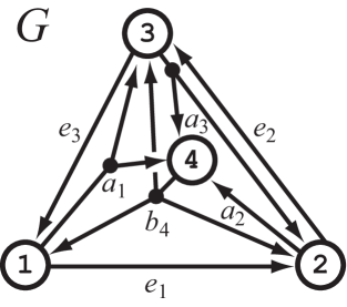
Figure 47: A graph with four states $\{1,2,3,4\}$, four deterministic actions $\{e_{1},e_{2},e_{3},a_{2}\}$, and three nondeterministic actions $\{a_{1},a_{3},b_{4}\}$.

Figure 47 shows a fully controllable nondeterministic graph on four states. The graph contains four deterministic actions and three nondeterministic actions.

Three of the deterministic actions form a directed cycle: $1\xrightarrow{e_{1}}2\xrightarrow{e_{2}}3\xrightarrow{e_{3}}1$. The remaining deterministic action, $a_{2}$, moves from state 2 to state 4.

Actions $a_{1}$, $a_{3}$, and $b_{4}$ are nondeterministic. Action $a_{1}$ moves nondeterministically from state 1 to either state 3 or state 4, while action $a_{3}$ moves nondeterministically from state 3 to either state 2 or state 4. Finally, action $b_{4}$ moves nondeterministically back from state 4 to any of the other three states.

Figure 48 shows relation $A$ for the graph of Figure 47, with $A$ as defined in Lemma 30 on page 30. As indicated in the figure, some maximal strategies have two-state goals. In addition, two of the maximal strategies converge to the same singleton goal, namely state $4$.

$\begin{array}[]{c|ccccccc}A&e_{1}&e_{2}&e_{3}&a_{1}&a_{2}&a_{3}&b_{4}\\[2.0pt] \hline\cr\sigma_{1}&&\bullet&\bullet&&&&\bullet\\[2.0pt] \sigma_{2}&\bullet&&\bullet&&&&\bullet\\[2.0pt] \sigma_{3}&\bullet&\bullet&&&&&\bullet\\[2.0pt] \sigma_{4}&\bullet&&\bullet&&\bullet&\bullet&\\[2.0pt] \sigma_{5}&\bullet&&&\bullet&\bullet&\bullet&\\[2.0pt] \sigma_{14}&&\bullet&\bullet&&\bullet&&\\[2.0pt] \sigma_{34}&\bullet&\bullet&&\bullet&\bullet&&\\[2.0pt] \end{array}$

$\begin{array}[]{c}\hbox{Goal}\\[2.0pt] \hline\cr 1\\[2.0pt] 2\\[2.0pt] 3\\[2.0pt] 4\\[2.0pt] 4\\[2.0pt] \{1,4\}\\[2.0pt] \{3,4\}\\[2.0pt] \end{array}$

Figure 48: Relation $A$ describes the strategy complex for the graph of Figure 47 in terms of its maximal strategies and their constituent actions. The rightmost column further shows each maximal strategy’s goal. Observe that some strategies converge to multi-state goals.

$\begin{array}[]{c|cccc}Q&e_{1}&a_{1}&a_{2}&a_{3}\\[2.0pt] \hline\cr\sigma_{2}&\bullet&&&\\[2.0pt] \sigma_{3}&\bullet&&&\\[2.0pt] \sigma_{4}&\bullet&&\bullet&\bullet\\[2.0pt] \sigma_{14}&&&\bullet&\\[2.0pt] \sigma_{34}&\bullet&\bullet&\bullet&\\[2.0pt] \end{array}$

$\begin{array}[]{c}\hbox{Goal}\\[2.0pt] \hline\cr 2\\[2.0pt] 3\\[2.0pt] 4\\[2.0pt] \{1,4\}\\[2.0pt] \{3,4\}\\[2.0pt] \end{array}$

Figure 49: Relation $Q$ models $\mathop{\rm Lk}(\Psi_{A},\sigma_{5})$, with $A$ as in Figure 48.

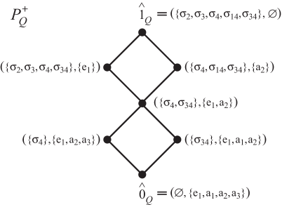
Figure 50: The Galois lattice $P^{+}_{Q}$ has length 4, with $Q$ as in Figure 49.

Strategies $\sigma_{1}$, $\sigma_{2}$, $\sigma_{3}$, and $\sigma_{4}$ each have (at least) six different informative action release sequences of length (at least) 3, as guaranteed to exist in $\Delta_{G}$ by Theorem 32. Strategy $\sigma_{5}$ also has informative action release sequences of length at least 3 (in fact, length 4), but it only has four such sequences, consistent with the comments on page 13.2. We can see this by constructing the Galois lattice $P^{+}_{Q}$, with $Q$ modeling $\mathop{\rm Lk}(\Psi_{A},\sigma_{5})$. Figures 49 and 50 depict $Q$ and $P^{+}_{Q}$, respectively. There are indeed four downward paths of length 4 from $\hat{1}_{Q}$ to $\hat{0}_{Q}$.

In order to delay identification of $\sigma_{5}$ as long as possible, the lattice $P^{+}_{Q}$ further tells us that one should reveal action $a_{2}$ either right away or right after first revealing action $e_{1}$. However, as soon as one has revealed action $a_{2}$, an observer knows that the goal is either state 4 or a two-state set containing state 4. If the observer has adversarial control over the outcome of nondeterministic actions in $G$, then as soon as one has revealed two of $\sigma_{5}$’s actions, the observer-adversary can lie in wait for the system at state 4.

Of course, as indicated on page • ‣ 13.2, one can delay goal recognition for 3 steps if one is free to choose any strategy for that goal. For goal state 4, one should choose strategy $\sigma_{4}$ rather than $\sigma_{5}$, and reveal actions $e_{1}$, $e_{3}$, $a_{2}$, either in that order or in the order $e_{3}$, $e_{1}$, $a_{2}$.

13.4 Randomization

Suppose $G=(V,{\mathfrak{A}})$ is a fully controllable graph with $\lvert V\rvert=\lvert{\mathfrak{A}}\rvert=n>1$. These conditions imply that there is exactly one action at each state and that the maximal simplices of $\Delta_{G}$ consist of all subsets of ${\mathfrak{A}}$ of size $n-1$. Consequently, $\Delta_{G}$ is a boundary complex, specifically $\Delta_{G}={\partial{({\mathfrak{A}})}}$. As we have seen, such complexes preserve attribute privacy, meaning it is impossible to infer any additional actions from actions already revealed. The existence of $(n-1)!$ different informative action release sequences of length $n-1$ for any given maximal strategy here simply means that one may reveal the actions of that strategy in any order.

The technical complications discussed previously arise when there are multiple actions at some or all states of $V$. One may circumvent such complications by creating a single “effective action” at each state, for instance by choosing stochastically among the given actions available at a state when the system is in that state. The precise probabilities are not significant from the perspective of combinatorial strategy obfuscation, so long as the probability of choosing any given original action is greater than 0, and all such probabilities sum to 1. (Of course, the actual probabilities will affect the expected time to attain the goal.)

A related issue concerns execution order versus release order. The privacy results in this report assume that a system can control the order in which it reveals actions. If instead actions are revealed as they are executed, then an observer may be able to infer the underlying strategy more quickly than desired. In order to obfuscate the strategy, the system may need to be willing to ignore early arrival at the goal and instead continue moving. The precise criteria determining whether the system stops or continues could be stochastic, or could reflect a protocol determined by the desired action release sequence.

14 Relations as a Category

We have discussed disinformation, obfuscation, and other manipulation of relations. The goal of such transformations has been to preserve privacy by removing or hiding free faces. We have not yet discussed such transformations formally. For instance, the coordinate transformations of Section 9 raise the question:

How should one think about maps between relations?

14.1 Relationship-Preserving Morphisms

Traditionally, relations are themselves morphisms between sets (with functions a special case). In thinking about privacy, it is useful to define a category in which relations are the objects. We have some choices in defining morphisms for this category. Bearing in mind our Dowker constructions (see again Definition 1 on page 1), we adopt the following standard definition:

Notation:

(1) We frequently will be working with two relations: $R$ is a relation on $X^{R}\times Y^{R}$ and $Q$ is a relation on $X^{Q}\times Y^{Q}$ (the superscripts are just indices to indicate the underlying relation). In order to distinguish rows and columns between the two relations, we will also use notation of the form $X^{R}_{y}$, $Y^{R}_{x}$, $X^{Q}_{y}$, and $Y^{Q}_{x}$.  (2) By a set map  we mean a function between two sets.

Definition 33 (Morphism).

Let $R$ be a relation on $X^{R}\times Y^{R}$ and let $Q$ be a relation on $X^{Q}\times Y^{Q}$.  A morphism of relations  $f:R\rightarrow Q$ is a pair of set maps:

$$f_{X} : X^{R}\rightarrow X^{Q}$$

$$f_{Y} : Y^{R}\rightarrow Y^{Q}$$

such that $\big{(}f_{X}(x),\,f_{Y}(y)\big{)}\in Q$ whenever $(x,y)\in R$.

In other words, a morphism of relations maps individuals to individuals and attributes to attributes in a way that preserves relationships.

The following lemma follows from the definitions (a proof appears in Appendix I.1):

Lemma 34 (Induced Simplicial Maps).

A morphism $f:R\rightarrow Q$ between nonvoid relations induces simplicial maps between the Dowker complexes:

$$f_{X} : \Psi_{R}\rightarrow\Psi_{Q}$$

$$f_{Y} : \Phi_{R}\rightarrow\Phi_{Q}$$

Notational comment:

The symbols $f_{X}$ and $f_{Y}$ are overloaded intentionally. The simplicial map $f_{X}$ is precisely the set map $f_{X}$ applied to the vertices of any simplex:  If $\sigma=\{x_{0},\ldots,x_{k}\}\in\Psi_{R}$, then $f_{X}(\sigma)=\{f_{X}(x_{0}),\ldots,f_{X}(x_{k})\}\in\Psi_{Q}$. Similarly for $f_{Y}$.

Connectivity Implication:  Intuitively, one cannot partition the individuals of a connected relation into two or more pairwise disjoint classes without misclassifying some individuals or ignoring some relationships. A graph connectivity argument provides a possible proof. Lemma 34 provides another, with additional insight.  Let us look at some examples:

Two Bits onto One:

Consider again the relations $S$ and $Q$ of Figures 15 and 16, respectively, on page 15. Relation $S$ models a one-bit relation — an attribute and its negation. Relation $Q$ models a two-bit relation — two attributes and their negations. The Dowker complexes for $S$ have $\mathbb{S}^{\kern 0.56001pt{0}}$ homotopy type, while those for $Q$ have $\mathbb{S}^{1}$ homotopy type. We can think of $S$ as a classification, splitting individuals into those that have some attribute ${\tt a}$ and those that do not.

By Lemma 34, a morphism $f:Q\rightarrow S$ induces simplicial (hence continuous) maps between the corresponding Dowker complexes of $S$ and $Q$. Since $\mathbb{S}^{1}$ is connected but $\mathbb{S}^{\kern 0.56001pt{0}}$ is not, there is no surjective continuous function from $\mathbb{S}^{1}$ to $\mathbb{S}^{\kern 0.56001pt{0}}$. Consequently, no morphism $f:Q\rightarrow S$ can truly be a classification: $f_{Y}$ can map all four attributes $\{{\tt a},\neg{\tt a},{\tt b},\neg{\tt b}\}$ of $Q$ to the single attribute ${\tt a}$ or all four attributes to $\neg{\tt a}$, but $f_{Y}$ cannot map to both ${\tt a}$ and $\neg{\tt a}$.

$\begin{array}[]{c|cccc}\hbox{\large$\;Q^{\prime}$}&{\tt a}&\neg{\tt a}\\[2.0pt] \hline\cr 1&\bullet&\\ 2&\bullet&\\ 3&&\bullet\\ 4&&\bullet\\ \end{array}$

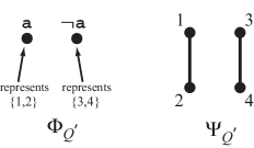
Figure 51: Relation $Q^{\prime}$ obtained from relation $Q$ of Fig. 16 by discarding attributes ${\tt b}$ and $\neg{\tt b}$.

This impossibility may at first seem paradoxical. After all, one can simply cut relation $Q$ down the middle and throw away the columns involving attributes ${\tt b}$ and $\neg{\tt b}$, as shown in Figure 51. After that, a surjective morphism $f^{\prime}:Q^{\prime}\rightarrow S$ is immediate. Indeed, that is possible. However, in so doing, one has discarded some relationships, perhaps purposefully, perhaps accidentally. In particular, the relationship between individuals #1 and #3 of $Q$ via attribute ${\tt b}$ is lost, as is the relationship between individuals #2 and #4 via attribute $\neg{\tt b}$. This reasoning simply underscores the fact that morphisms of relations preserve relationships. Lack of continuity in a function therefore is a sign that one is discarding some relationships. Whether such discard is desirable depends on one’s goals in a particular application.

Three Bits onto Two:

Recall as well Figure 17 on page 17, which depicts a three-bit relation $R$ — three attributes and their negations, capable of distinguishing between eight individuals. The homotopy type of the Dowker complexes is $\mathbb{S}^{2}$. With $Q$ as above, the following question arises naturally when trying to reduce complexity of data yet preserve information:

Does there exist a surjective morphism $f:R\rightarrow Q$ ?

Unlike the previous example, there do exist continuous maps from $\mathbb{S}^{2}$ onto $\mathbb{S}^{1}$, so perhaps one can find a surjective morphism $f:R\rightarrow Q$.  In fact, one can not. Intuitively, the issue is that the two-dimensional relationships of $R$ try to fill the one-dimensional hole of relation $Q$.  Here is a simplex-based argument:

• Suppose surjective $f:R\rightarrow Q$ exists. As will be discussed later (see page 35), this means the component functions $f_{X}:X^{R}\rightarrow X^{Q}$ and $f_{Y}:Y^{R}\rightarrow Y^{Q}$ are surjective as set maps.

• One may therefore assume without loss of generality that $f_{Y}({\tt a})={\tt a}$ and $f_{Y}({\tt b})={\tt b}$.

• The triangles $\{{\tt a},{\tt b},{\tt c}\}$ and $\{{\tt a},{\tt b},\neg{\tt c}\}$ are both simplices in $\Phi_{R}$. The maximal simplices of $\Phi_{Q}$ are edges.

• By Lemma 34, this means that $f_{Y}({\tt c})$ and $f_{Y}(\neg{\tt c})$ are both elements of $\{{\tt a},{\tt b}\}$ in $\Phi_{Q}$.

• Again by surjectivity, we therefore see that $\{f_{Y}(\neg{\tt a}),f_{Y}(\neg{\tt b})\}=\{\neg{\tt a},\neg{\tt b}\}$.

• Another triangle-versus-edge argument then says that $f_{Y}({\tt c})$ and $f_{Y}(\neg{\tt c})$ are both elements of $\{\neg{\tt a},\neg{\tt b}\}$, giving us a contradiction.

Of course, as in constructing $Q^{\prime}$ of Figure 51, if we are willing to tolerate discontinuities, we could discard one attribute and its negation to obtain $Q$ from $R$. As before, discontinuity means losing awareness of some relationship(s). For instance, if we omit attribute ${\tt c}$, we would become unaware in $Q$ of the relationship that exists in $R$ among the set of individuals $\{1,3,5,7\}$.

14.2 Privacy-Establishing Morphisms

$\begin{array}[]{c|ccccc}\hbox{\large$M$}&{\tt a}&{\tt b}&{\tt c}&{\tt d}&{\tt e}\\[2.0pt] \hline\cr 1&\bullet&\bullet&&&\bullet\\ 2&\bullet&\bullet&\bullet&&\\ 3&&\bullet&\bullet&\bullet&\\ 4&&&\bullet&\bullet&\bullet\\ 5&\bullet&&&\bullet&\bullet\\ \end{array}$

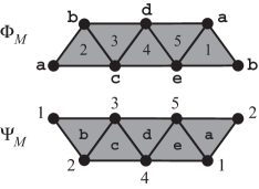
Figure 52: Relation $M$ is isomorphic to relation $G$ of Figure 23 on page 23, now without the author-book semantics. The Dowker complexes are dual triangulations of the Möbius strip, with $\mathbb{S}^{1}$ homotopy type.

Relations involve two spaces. Looking at just $\Phi_{R}$ or just $\Psi_{R}$ may hide some interesting properties. For instance, consider the Möbius strip relation $M$ of Figure 52. We encountered this relation previously, in Section 10.

We might wish to remove some of the inferences discussed in Section 10 by reshaping the underlying relation without discarding any relationships. Doing so leads to the following question:

Does there exist a surjective morphism $f:M\rightarrow T$, with $T$ a relation that preserves both attribute and association privacy ?

If such a morphism $f$ exists, then, as we mentioned in Sections 5 and 8, relation $T$ must have the topology of either a linear cycle or a spherical boundary complex. It turns out that the answer to the question above is “yes”, with $T$ being a relation whose Dowker complexes are boundaries of tetrahedra (see Figure 30 on page 30).

This construction is not immediately obvious from the complexes $\Phi_{M}$ and $\Psi_{M}$. Although those simplicial complexes are 2-dimensional, suggesting that their triangles can be wrapped around a tetrahedron, doing so actually collapses two of the five triangles to edges. Indeed, the component functions for one such surjective morphism $f:M\rightarrow T$ are:

$$f_{X}\;:\;X^{M} \rightarrow X^{T}$$

$$1 \mapsto 4$$

$$2 \mapsto 1$$

$$3 \mapsto 2$$

$$4 \mapsto 3$$

$$5 \mapsto 4$$

$$f_{Y}\;:\;Y^{M} \rightarrow Y^{T}$$

$${\tt a} \mapsto {\tt a}$$

$${\tt b} \mapsto {\tt b}$$

$${\tt c} \mapsto {\tt c}$$

$${\tt d} \mapsto {\tt d}$$

$${\tt e} \mapsto {\tt a}$$

The induced simplicial maps act on the five maximal simplices of $\Psi_{M}$ and $\Phi_{M}$ as follows:

$$f_{X}\;:\;\Psi_{M} \rightarrow \Psi_{T}$$

$$\{1,2,3\} \mapsto \{1,2,4\}$$

$$\{2,3,4\} \mapsto \{1,2,3\}$$

$$\{3,4,5\} \mapsto \{2,3,4\}$$

$$\{1,4,5\} \mapsto \{3,4\}$$

$$\{1,2,5\} \mapsto \{1,4\}$$

$$f_{Y}\;:\;\Phi_{M} \rightarrow \Phi_{T}$$

$$\{{\tt a},{\tt b},{\tt c}\} \mapsto \{{\tt a},{\tt b},{\tt c}\}$$

$$\{{\tt b},{\tt c},{\tt d}\} \mapsto \{{\tt b},{\tt c},{\tt d}\}$$

$$\{{\tt c},{\tt d},{\tt e}\} \mapsto \{{\tt a},{\tt c},{\tt d}\}$$

$$\{{\tt a},{\tt d},{\tt e}\} \mapsto \{{\tt a},{\tt d}\}$$

$$\{{\tt a},{\tt b},{\tt e}\} \mapsto \{{\tt a},{\tt b}\}$$

Even though $f_{X}$ and $f_{Y}$ are surjective as set maps on the vertices of the Dowker complexes, they are not  surjective as simplicial maps on the complexes themselves. Each only covers three of the four triangles comprising the tetrahedron in its codomain. At first glance it may therefore seem that the morphism $f:M\rightarrow T$ resulting from $f_{X}$ and $f_{Y}$ does not achieve the desired privacy preservation. A closer look, however, reveals that $f$ is actually surjective as a map of relations: it maps the elements of $M\!$ onto the elements of $T$. Therefore, it does represent a transformation that achieves privacy preservation.

In order to understand this paradox, imagine again that $M$ represents an authorship database. Think of the maps $f_{X}$ and $f_{Y}$ as quotient maps, in this case equating authors 1 and 5 and books ${\tt a}$ and ${\tt e}$. The equivalencing of authors might constitute a recognition of pseudonyms. The equivalencing of books might represent a generalization from titles to genres. Such changes of resolution, carefully chosen, perhaps based on external structure, can preserve relationships while reducing recognition and inference granularity.

14.3 Summary of Morphism Properties

Definition 33 defines a morphism of relations $f:R\rightarrow Q$ in terms of underlying set functions $f_{X}:X^{R}\rightarrow X^{Q}$ and $f_{Y}:Y^{R}\rightarrow Y^{Q}$. These set functions further induce simplicial maps $f_{X}:\Psi_{R}\rightarrow\Psi_{Q}$ and $f_{Y}:\Phi_{R}\rightarrow\Phi_{Q}$. The previous subsections spoke of surjectivity in varying contexts. Similarly, one could speak of maps as being injective in varying contexts. Finally, one also speaks of morphisms as being epimorphisms and monomorphisms. This subsection summarizes how these properties relate for the various maps.  See Appendix I.1 for proofs.

First, some definitional context and reminders:

• A morphism of relations $f:R\rightarrow Q$ is also a set map between the set of pairs comprising $R$ and the set of pairs comprising $Q$. Specifically, $f(x,y)=(f_{X}(x),f_{Y}(y))$ for all $(x,y)\in R$.

  One may speak of $f$ as being surjective and/or injective, meaning as a set map.

• We say that two morphisms of relations $g,h:R\rightarrow Q$ are equal, written $g=h$, when they are equal as set maps of ordered pairs, meaning $g(x,y)=h(x,y)$ for all $(x,y)\in R$.

  (Note: If $R$ contains blank rows and/or columns, then $g=h$ is possible even though $g_{X}\neq h_{X}$ and/or $g_{Y}\neq h_{Y}$, as set maps. This will not cause us problems; one could pass to equivalence classes in Definition 33.)

• The functions $f_{X}:X^{R}\rightarrow X^{Q}$ and $f_{Y}:Y^{R}\rightarrow Y^{Q}$ are set maps. One may speak of them as being surjective and/or injective.

• One may also ask whether the induced simplicial maps $f_{X}:\Psi_{R}\rightarrow\Psi_{Q}$ and $f_{Y}:\Phi_{R}\rightarrow\Phi_{Q}$ are surjective and/or injective as maps between simplicial complexes viewed as sets.

• Suppose $f:R\rightarrow Q$ is a morphism of relations. Recall from category theory that $f$ is an epimorphism if, for any pair of morphisms $g,h:Q\rightarrow S$,  $g\circ f=h\circ f$ implies $g=h$.

  Recall further that a morphism $f:R\rightarrow Q$ is a monomorphism if, for any pair of morphisms $g,h:S\rightarrow R$, $f\circ g=f\circ h$ implies $g=h$.

Lemma 35 (Morphism Properties).

Assume the notation from above and that all relevant relations are nonvoid. Let $f:R\rightarrow Q$ be a morphism of relations (as per Definition 33). Then:

• $f_{X}$ and $f_{Y}$ are injective set maps $\implies$ $f$ is injective $\iff$ $f$ is a monomorphism.

• $f$ surjective $\implies$ $f$ epimorphism $\iff$ $f_{X}$ and $f_{Y}$ are surjective set maps.

  (Additional conditions for that last $\iff$: The $\Longrightarrow$ direction assumes that $Q$ has no blank rows or columns, while the $\Longleftarrow$ direction assumes that $R$ has no blank rows or columns.)

The two uni-directional implications $\implies$ above are strict.

• If $f_{X}:\Psi_{R}\rightarrow\Psi_{Q}$ is surjective and $Q$ has no blank rows, then $f_{X}:X^{R}\rightarrow X^{Q}$ is surjective.

  Similarly for $f_{Y}$, now assuming that $Q$ has no blank columns.

  The converses need not hold. Indeed, $f$ itself can be surjective but the maps of simplicial complexes need not be (as we saw with the maps of page 14.2).

• If $f_{X}:X^{R}\rightarrow X^{Q}$ is injective, then $f_{X}:\Psi_{R}\rightarrow\Psi_{Q}$ is injective. The converse holds if $R$ has no blank rows.

  Similarly for $f_{Y}$, now assuming that $R$ has no blank columns for the converse.

14.4 G-Morphisms

Since a relation $R$ defines a poset $P_{R}$, rather than merely create morphisms from set maps between individuals and attributes as in Definition 33, we may broaden the definition by considering maps between posets:

Definition 36 (G-Morphism).

Let $R$ and $Q$ be nonvoid relations.
           A  G-morphism  $f:R\rightarrow Q$  is any poset map  $f:P_{R}\rightarrow P_{Q}$.

Comments:

The “G” stands for “Galois”. We might have insisted that a G-morphism $R\rightarrow Q$ be a lattice morphism $P^{+}_{R}\rightarrow P^{+}_{Q}$ rather than merely a poset map $P_{R}\rightarrow P_{Q}$, but that might be too restrictive. Instead, as subsequent lemmas will describe, we view a G-morphism as providing homotopy flexibility. In particular, a morphism between relations as per Definition 33 induces two homotopic G-morphisms. The lattice structure of the codomain is relevant, in that it allows one to fill in elements not directly in the image of any one G-morphism, as will become apparent in Theorem 41.

$$\begin{CD}{\mathfrak{F}}(\Psi_{R})@>{\hskip 21.68121ptf_{X}\hskip 21.68121pt}>{}>\hskip 3.61371pt{\mathfrak{F}}(\Psi_{Q})\\[3.0pt] @V{\phi_{R}}V{}V@A{}A{\psi_{R}}A@V{\phi_{Q}}V{}V@A{}A{\psi_{Q}}A\\ {\mathfrak{F}}(\Phi_{R})@>{\hskip 21.68121ptf_{Y}\hskip 21.68121pt}>{}>\hskip 3.61371pt{\mathfrak{F}}(\Phi_{Q})\\[3.0pt] \end{CD}$$

Figure 53: Diagram showing the poset maps $f_{X}$ and $f_{Y}$ induced by a morphism $f:R\rightarrow Q$, along with the homotopy equivalences between each relation’s face posets. (The diagram need not be commutative, but is almost so; see Lemma 37.)

Recall that a morphism $f:R\rightarrow Q$ as per Definition 33 is built from two set maps $f_{X}$ and $f_{Y}$ and that these set maps induce simplicial maps between the Dowker complexes, as per Lemma 34. We may therefore further regard $f_{X}$ and $f_{Y}$ as order-preserving poset maps between the face posets of the Dowker complexes: $f_{X}:{\mathfrak{F}}(\Psi_{R})\rightarrow{\mathfrak{F}}(\Psi_{Q})$ and $f_{Y}:{\mathfrak{F}}(\Phi_{R})\rightarrow{\mathfrak{F}}(\Phi_{Q})$. Consequently, we have a diagram of maps as in Figure 53. The diagram need not be commutative, but the following containments hold:

Lemma 37 (Witness Containment).

Let $f:R\rightarrow Q$ be a morphism of nonvoid relations. Then:

• $(f_{Y}\circ\phi_{R})(\sigma)\;\subseteq\;(\phi_{Q}\circ f_{X})(\sigma)$,  for every $\sigma\in\Psi_{R}$,

• $(f_{X}\circ\psi_{R})(\gamma)\;\subseteq\;(\psi_{Q}\circ f_{Y})(\gamma)$,  for every $\gamma\in\Phi_{R}$.

(See Appendix I.2 for a proof of the previous lemma and its upcoming corollaries.)

As a corollary, we see that the diagram of Figure 53 describes two pairs of homotopic maps:

Corollary 38 (Homotopic Face Maps).

Let $f:R\rightarrow Q$ be a morphism of nonvoid relations. Then:

• $f_{X}$ and $\,\psi_{Q}\circ f_{Y}\circ\phi_{R}$ are homotopic poset maps $\,{\mathfrak{F}}(\Psi_{R})\rightarrow{\mathfrak{F}}(\Psi_{Q})$,

• $f_{Y}$ and $\,\phi_{Q}\circ f_{X}\circ\psi_{R}$ are homotopic poset maps $\,{\mathfrak{F}}(\Phi_{R})\rightarrow{\mathfrak{F}}(\Phi_{Q})$.

The images of the compositions that appear in Corollary 38 may be regarded as lying in $P_{Q}$. We may further restrict the domain of these maps to be $P_{R}$, giving us the following G-morphisms:

Definition 39 (Induced G-Morphisms).

A morphism of nonvoid relations $f:R\rightarrow Q$ induces two G-morphisms $R\rightarrow Q$, defined by the following poset maps $P_{R}\rightarrow P_{Q}$:

$$f_{X}^{g}\;=\;(\psi_{Q}\circ f_{Y}\circ\phi_{R})|_{P_{R}}\qquad\qquad f_{Y}^{g}\;=\;(\phi_{Q}\circ f_{X}\circ\psi_{R})|_{P_{R}}.$$

(The “$g$” superscript stands for “Galois” while the vertical bar “$|$” means “restricted to”. See also Appendix I.2.)

Corollary 40 (Homotopic G-Morphisms).

Let $f:R\rightarrow Q$ be a morphism of nonvoid relations. The induced G-morphisms given by the poset maps $f_{X}^{g},f_{Y}^{g}:P_{R}\rightarrow P_{Q}$ are homotopic.

The proof of Corollary 40 on page I.2 says that we may view the underlying maps $f_{X}$ and $f_{Y}$ of a morphism $f$ as mapping any inference-closed set (viewed either as a set of individuals or as a set of attributes) from the domain of $f$ to an interval (in the poset sense) of inference-closed sets in the codomain of $f$.

$\begin{array}[]{c|c}\hbox{\large$R$}&{\tt a}\\[2.0pt] \hline\cr 1&\bullet\\ \end{array}$

$\begin{array}[]{c|cc}\hbox{\large$Q$}&{\tt a}&{\tt b}\\[2.0pt] \hline\cr 1&\bullet&\bullet\\ 2&\bullet&\\ \end{array}$

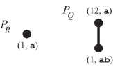
Figure 54: Relation $R$ is a subrelation of $Q$. How should one embed $P_{R}$ into $P_{Q}$? There are two possible embeddings, related by a homotopy.

For a simple example, see Figure 54. One may regard relation $R$ as a subrelation of $Q$, then define $f:R\rightarrow Q$ to be inclusion. For instance, maybe $R$ and $Q$ represent individuals #1 and #2 at two parties ${\tt a}$ and ${\tt b}$, with $R$ representing known parties and party-attendees at some time and $Q$ representing an update of that information at a later time. Observe that:

$$f_{X}^{g}((1,{\tt a}))\! = \!(\psi_{Q}\circ f_{Y}\circ\phi_{R})(\{1\})\;=\;(\psi_{Q}\circ f_{Y})(\{{\tt a}\})\;=\;\psi_{Q}(\{{\tt a}\})\;=\;\{1,2\}\;\;\hbox{``$=$''}\;\;(12,{\tt a}),$$

$$f_{Y}^{g}((1,{\tt a}))\! = \!(\phi_{Q}\circ f_{X}\circ\psi_{R})(\{{\tt a}\})\;=\;(\phi_{Q}\circ f_{X})(\{1\})\;=\;\phi_{Q}(\{1\})\;=\;\{{\tt a},{\tt b}\}\;\;\hbox{``$=$''}\;\;(1,{\tt a}{\tt b}).$$

The last equality in each row indicates how to view the image element on the left of the “$=$” as an element of the poset $P_{Q}$.

Both $f_{X}^{g}$ and $f_{Y}^{g}$ tell us how to update inference-closed sets from $P_{R}$ into inference-closed sets within $P_{Q}$:

• The map $f_{X}^{g}$ updates associations while holding observed attributes fixed. In this example, based on initial information (relation $R$), we know that person #1 attended party ${\tt a}$. Once we update that information (relation $Q$) we can conclude that person #2 also attended a party at which person #1 was present.

• Similarly, the map $f_{Y}^{g}$ updates attributes while holding observed individuals fixed. In this example, updated information allows us to conclude that person #1 attended not only party ${\tt a}$ but also party ${\tt b}$.

In general, for any fixed element of $P_{R}$, the two maps may give different results, but those results are comparable in $P_{Q}$. Here $f$ was inclusion, so we could speak of holding attributes or individuals “fixed”. More generally, “fixed” is replaced by whatever $f$ does.

14.5 Surjectivity Revisited

A paradox: We saw on page 52 a surjective morphism $f$, from the Möbius strip relation of Figure 52 to the tetrahedral relation of Figure 30, whose induced simplicial maps $f_{X}:\Psi_{M}\rightarrow\Psi_{T}$ and $f_{Y}:\Phi_{M}\rightarrow\Phi_{T}$ were not surjective. This raises some questions:

1. Are the induced poset maps $f_{X}^{g},f_{Y}^{g}:P_{M}\rightarrow P_{T}$ surjective?

2. If not, how can one speak of a surjective morphism?

(Note that $P^{+}_{M}$ is isomorphic to $P^{+}_{G}$ as shown in Figure 25 on page 25. A rendering would be identical, except for lowercase letters in place of uppercase ones. The lattice $P^{+}_{T}$ appears in Figure 31 on page 31.)

The answer to Question 1 is that the two poset maps are not  surjective. Observe in Table 9 on page 9, for instance, that the image of $f_{X}^{g}$ does not include $(4,{\tt a}{\tt b}{\tt d})$. Similarly, the image of $f_{Y}^{g}$ does not include $(134,{\tt a})$.

These missing elements are in the image of both maps together, viewed as a pair of homotopic maps, as per Corollary 40. Unfortunately, that explanation is not a full answer to Question 2. For instance, neither map’s image includes the element $(13,{\tt a}{\tt c})$ of $P_{T}$, nor does that element appear in any interval $[f_{Y}^{g}(p),f_{X}^{g}(p)]$ as $p$ varies throughout $P_{M}$.

To answer question 2, the lattice structure of $P_{T}$ is useful. In the example, the image of $f_{X}^{g}$ includes all elements of $P_{T}$ that correspond to maximal simplices of $\Psi_{T}$. Similarly, the image of $f_{Y}^{g}$ includes all elements of $P_{T}$ that correspond to maximal simplices of $\Phi_{T}$. Intuitively, we therefore expect that the lattice operations (which correspond to intersection in either $\Psi_{T}$ or $\Phi_{T}$) will generate all the elements of $P_{T}$. In that sense, the surjectivity of $f$ appears as surjectivity of each of $f_{X}^{g}$ and $f_{Y}^{g}$, once one completes their images under lattice operations.

$\begin{array}[]{ccccc}p&&f_{X}^{g}(p)&&f_{Y}^{g}(p)\\[3.0pt] \hline\cr$(\makebox[21.0pt][l]{{12}}, \makebox[21.0pt][r]{{{\tt a}{\tt b}}})$&&$(\makebox[21.0pt][l]{{14}}, \makebox[21.0pt][r]{{{\tt a}{\tt b}}})$&&$(\makebox[21.0pt][l]{{14}}, \makebox[21.0pt][r]{{{\tt a}{\tt b}}})$\\[2.0pt] $(\makebox[21.0pt][l]{{2}}, \makebox[21.0pt][r]{{{\tt a}{\tt b}{\tt c}}})$&&$(\makebox[21.0pt][l]{{1}}, \makebox[21.0pt][r]{{{\tt a}{\tt b}{\tt c}}})$&&$(\makebox[21.0pt][l]{{1}}, \makebox[21.0pt][r]{{{\tt a}{\tt b}{\tt c}}})$\\[2.0pt] $(\makebox[21.0pt][l]{{123}}, \makebox[21.0pt][r]{{{\tt b}}})$&&$(\makebox[21.0pt][l]{{124}}, \makebox[21.0pt][r]{{{\tt b}}})$&&$(\makebox[21.0pt][l]{{124}}, \makebox[21.0pt][r]{{{\tt b}}})$\\[2.0pt] $(\makebox[21.0pt][l]{{23}}, \makebox[21.0pt][r]{{{\tt b}{\tt c}}})$&&$(\makebox[21.0pt][l]{{12}}, \makebox[21.0pt][r]{{{\tt b}{\tt c}}})$&&$(\makebox[21.0pt][l]{{12}}, \makebox[21.0pt][r]{{{\tt b}{\tt c}}})$\\[2.0pt] $(\makebox[21.0pt][l]{{3}}, \makebox[21.0pt][r]{{{\tt b}{\tt c}{\tt d}}})$&&$(\makebox[21.0pt][l]{{2}}, \makebox[21.0pt][r]{{{\tt b}{\tt c}{\tt d}}})$&&$(\makebox[21.0pt][l]{{2}}, \makebox[21.0pt][r]{{{\tt b}{\tt c}{\tt d}}})$\\[2.0pt] $(\makebox[21.0pt][l]{{234}}, \makebox[21.0pt][r]{{{\tt c}}})$&&$(\makebox[21.0pt][l]{{123}}, \makebox[21.0pt][r]{{{\tt c}}})$&&$(\makebox[21.0pt][l]{{123}}, \makebox[21.0pt][r]{{{\tt c}}})$\\[2.0pt] $(\makebox[21.0pt][l]{{34}}, \makebox[21.0pt][r]{{{\tt c}{\tt d}}})$&&$(\makebox[21.0pt][l]{{23}}, \makebox[21.0pt][r]{{{\tt c}{\tt d}}})$&&$(\makebox[21.0pt][l]{{23}}, \makebox[21.0pt][r]{{{\tt c}{\tt d}}})$\\[2.0pt] $(\makebox[21.0pt][l]{{4}}, \makebox[21.0pt][r]{{{\tt c}{\tt d}{\tt e}}})$&&$(\makebox[21.0pt][l]{{3}}, \makebox[21.0pt][r]{{{\tt a}{\tt c}{\tt d}}})$&&$(\makebox[21.0pt][l]{{3}}, \makebox[21.0pt][r]{{{\tt a}{\tt c}{\tt d}}})$\\[2.0pt] $(\makebox[21.0pt][l]{{345}}, \makebox[21.0pt][r]{{{\tt d}}})$&&$(\makebox[21.0pt][l]{{234}}, \makebox[21.0pt][r]{{{\tt d}}})$&&$(\makebox[21.0pt][l]{{234}}, \makebox[21.0pt][r]{{{\tt d}}})$\\[2.0pt] $(\makebox[21.0pt][l]{{45}}, \makebox[21.0pt][r]{{{\tt d}{\tt e}}})$&&$(\makebox[21.0pt][l]{{34}}, \makebox[21.0pt][r]{{{\tt a}{\tt d}}})$&&$(\makebox[21.0pt][l]{{34}}, \makebox[21.0pt][r]{{{\tt a}{\tt d}}})$\\[2.0pt] $(\makebox[21.0pt][l]{{5}}, \makebox[21.0pt][r]{{{\tt a}{\tt d}{\tt e}}})$&&$(\makebox[21.0pt][l]{{34}}, \makebox[21.0pt][r]{{{\tt a}{\tt d}}})$&&$(\makebox[21.0pt][l]{{4}}, \makebox[21.0pt][r]{{{\tt a}{\tt b}{\tt d}}})$\\[2.0pt] $(\makebox[21.0pt][l]{{145}}, \makebox[21.0pt][r]{{{\tt e}}})$&&$(\makebox[21.0pt][l]{{134}}, \makebox[21.0pt][r]{{{\tt a}}})$&&$(\makebox[21.0pt][l]{{34}}, \makebox[21.0pt][r]{{{\tt a}{\tt d}}})$\\[2.0pt] $(\makebox[21.0pt][l]{{15}}, \makebox[21.0pt][r]{{{\tt a}{\tt e}}})$&&$(\makebox[21.0pt][l]{{134}}, \makebox[21.0pt][r]{{{\tt a}}})$&&$(\makebox[21.0pt][l]{{4}}, \makebox[21.0pt][r]{{{\tt a}{\tt b}{\tt d}}})$\\[2.0pt] $(\makebox[21.0pt][l]{{1}}, \makebox[21.0pt][r]{{{\tt a}{\tt b}{\tt e}}})$&&$(\makebox[21.0pt][l]{{14}}, \makebox[21.0pt][r]{{{\tt a}{\tt b}}})$&&$(\makebox[21.0pt][l]{{4}}, \makebox[21.0pt][r]{{{\tt a}{\tt b}{\tt d}}})$\\[2.0pt] $(\makebox[21.0pt][l]{{125}}, \makebox[21.0pt][r]{{{\tt a}}})$&&$(\makebox[21.0pt][l]{{134}}, \makebox[21.0pt][r]{{{\tt a}}})$&&$(\makebox[21.0pt][l]{{14}}, \makebox[21.0pt][r]{{{\tt a}{\tt b}}})$\\[2.0pt] \end{array}$

Table 9: Each $p$ is of the form $(\sigma,\gamma)\in P_{M}$. The elements $f_{X}^{g}(p)$ and $f_{Y}^{g}(p)$ lie in $P_{T}$. See also Figures 25 and 31, on pages 25 and 31, respectively.  (As in those figures, the table elides commas and braces from set notation.  For Figure 25, recall that $M$ and $G$ are isomorphic relations.)

The following theorem summarizes the intuition of the previous pages:

Theorem 41 (Lattice Surjectivity).

Let $R$ and $Q$ be nonvoid relations with no blank rows or columns. Suppose $f:R\rightarrow Q$ is a surjective morphism (in the sense of Definition 33).  For any $q\in P_{Q}$:

$$q\;=\;\bigwedge_{j}\bigvee_{i}q_{ji},\quad\hbox{with each $q_{ji}$ in the image of $f_{X}^{g}:P_{R}\rightarrow P_{Q}$,}$$

$$q\;=\;\bigvee_{k}\bigwedge_{\ell}q^{\prime}_{k\ell},\quad\hbox{with each $q^{\prime}_{k\ell}$ in the image of $f_{Y}^{g}:P_{R}\rightarrow P_{Q}$.}$$

(Here, $\bigvee$ and $\bigwedge$ are the lattice operations of $P^{+}_{Q}$.)

See Appendix I.3 for a proof.

15 Future Thoughts

Throughout this report, one senses the inevitability of privacy loss, that the topology of relations necessarily converts attribute information into revealing gradient flow. Gradient flow appears both in the collapse of free faces [9] and in the lattice structure of information acquisition: Collapse of free faces infers unobserved attributes from observed attributes. The meet operation of a relation’s Galois lattice propels observed attributes into downward motion, toward minima of identification.  Still, alternatives exist.

15.1 Relaxing Assumptions

Gradient flow is a natural consequence of the assumptions stated in Section 3. Let us discuss briefly how to relax those assumptions, while leaving detailed explorations for the future.

1. We could drop the assumption of relational completeness. We might then observe a set of attributes $\gamma$ inconsistent with the given relation $R$, meaning $\gamma\not\in\Phi_{R}$. One possibility is that some individual in $R$ has attributes $\gamma$, but the relation does not capture this fact. There is another possibility, that $\gamma$ represents the attributes of some individual external to $R$. For instance, recall that in Lemma 12 a set of attributes inconsistent with a link’s relation identifies the linking set of individuals. Deciding between these two scenarios (new attributes for given individuals versus wholly new individuals) requires additional information, not so unlike the decisions faced in mapping unknown environments.

2. We could drop the assumption of observational monotonicity. We do wish to retain the ability to observe attributes asynchronously. However, we might be able to place algebraic structure on some attributes, so that certain newly observed attributes can cancel previously observed ones. Spending a dollar versus earning a dollar for instance. Such an algebraic structure would then permit upward motion in a relation’s Galois lattice. (This is not always possible, e.g., if a relation encodes history by time-indexing.)

3. We could drop the assumption of observational accuracy. Attributes frequently are measured by noisy sensors, whether based on physical instruments or errorful databases. Existing privacy work has frequently assumed noise intrinsically (e.g., identification in [17] was successful despite database errors). This report ignored noise in order to focus on the combinatorial structure of privacy. Presently, we will sketch a possible noise model, in which a sensor reports attributes stochastically. A sensor is a physical device and an interpretation algorithm, producing observed attributes $\gamma(t)$ as functions of time. Thus, as $t$ varies, $\gamma(t)$ may move either up or down in a relation’s Galois lattice, not just down.

   A caution: Moving from a purely combinatorial system to a stochastic system need not turn gradient flow into harmonic flow. Reasonable but noisy sensors create a (stochastic) gradient flow, by the Central Limit Theorem. Rather, a noisy sensor model in the observation of attributes facilitates the connection to other privacy work. For instance, one view of Differential Privacy [5] is that it injects noise into a sensor, with the noise magnitude chosen in part as a function of the time interval allotted for observations, thus preventing gradient flow from reaching a minimum. Moreover, adversarial control over $\gamma(t)$, perhaps by sensor disinformation, may be able to create more general flows.

15.2 Sensing Attributes Stochastically

We briefly explore a model for stochastic sensors within combinatorial relations, via a simple example. Consider relation $R$ of Figure 55. This relation produces Dowker complexes with $\mathbb{S}^{1}$ homotopy type, as indicated in the figure. The relation’s Galois lattice $P^{+}_{R}$ appears in Figure 56.

$\begin{array}[]{c|ccc}R&{\tt a}&{\tt b}&{\tt c}\\[2.0pt] \hline\cr 1&\bullet&\bullet&\\ 2&&\bullet&\bullet\\ 3&\bullet&&\bullet\\ \end{array}$

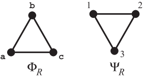
Figure 55: A relation whose Dowker complexes are dual triangulations of the circle. See Figure 56 for the associated Galois lattice.

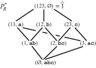
Figure 56: The lattice $P^{+}_{R}$ for relation $R$ of Figure 55. (We have elided commas and braces in sets.) — For later reference: The poset $P_{R}\cup\{\hat{1}\}$ consists of all elements in $P^{+}_{R}$ except for the bottom element, $(\emptyset,{\tt a}{\tt b}{\tt c})$.

Relation $R$’s space of attributes is $Y=\{{\tt a},{\tt b},{\tt c}\}$. Suppose that a sensor reports these attributes by observing the world and performing some computation. The report may be inaccurate. Such inaccuracy could be either adversarial or stochastic. We focus here on the stochastic case, and on one particular model: The sensor computes three probabilities, $p_{\tt a}$, $p_{\tt b}$, and $p_{\tt c}$, with $p_{y}$ being the probability that the sensor’s observation came from actual attribute $y\in Y$. These three probabilities constitute a point ${\bf{p}}=(p_{\tt a},p_{\tt b},p_{\tt c})$ in the full simplex $\{{\tt a},{\tt b},{\tt c}\}$, with the point’s barycentric coordinates being the three probabilities. Subsequently, the sensor reports an attribute by interpreting ${\bf{p}}$, perhaps by maximum probability. In order to reduce false positives, the sensor sets a confidence threshold below which it interprets ${\bf{p}}$ as too ambiguous. This thresholding carves the simplex $\{{\tt a},{\tt b},{\tt c}\}$ into four regions, one for each attribute, plus a zone of indecision. A sketch of this process appears in Figure 57.

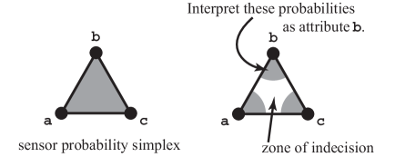
Figure 57: A sensor computes probabilities over a set of attributes $\{{\tt a},{\tt b},{\tt c}\}$. Left panel: A simplex whose vertices are those attributes models the possible distributions, with barycentric coordinates being probabilities. Right panel: An interpretation of probabilities as attributes, along with a zone of indecision, partitions the simplex into four regions.

Individuals in relation $R$ of Figure 55 have two attributes. One could model two observations as a probability distribution over ${Y}\mskip-2.5mu\times{Y}$. However, since the first observation may lead to an indecision, it is convenient to model the second observation as conditional on the first having produced a particular attribute. The second observation may: (i) repeat the just seen attribute, (ii) report an as yet unseen attribute, or (iii) fail to report anything. The net effect for (i) and (iii) is observation of one attribute. Consequently, the space of two observations may be interpreted as the first barycentric subdivision of the boundary of the attribute simplex, i.e., as $\mathop{\rm sd}({\partial{(Y)}})$, with the empty simplex modeling a zone of indecision. This process appears in Figure 58. One obtains a map from a stochastic sensor’s observations to the poset $P_{R}\cup\{\hat{1}\}$, with $\hat{1}$ representing an inability to decipher any attribute.  These calculations suggest that existing stochastic results fit naturally into this report’s combinatorial framework.

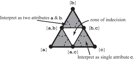
Figure 58: Two stochastic sensor observations may be modeled as a first observation followed by a conditional second observation. The resulting decision space has a representation isomorphic to the first barycentric subdivision of the boundary of the original probability simplex, with the empty simplex representing a zone of indecision. (The two observations may be understood as two points, ${\bf{p}}$ and ${\bf{q}}$, with ${\bf{p}}$ in the encompassing triangle and ${\bf{q}}$ in a shaded subtriangle.)

Appendix A Preliminaries

Assumption: All simplicial complexes, relations, posets, and lattices in this report are finite.

A.1 Simplicial Complexes

We largely follow the notation and definitions in [16] and [1].

• An (abstract) simplicial complex $\Sigma$ with underlying vertex set $X$ is a collection of finite subsets of $X$, such that if $\sigma$ is in $\Sigma$, then so is every subset of $\sigma$. An element of $\Sigma$ is called a simplex. We allow the empty set $\emptyset$ to be a simplex in $\Sigma$, for combinatorial reasons. An element of a simplex is called a vertex. It is also convenient to refer indistinguishably to any singleton simplex as a vertex. Not all elements of $X$ need to be vertices of $\Sigma$.

• The dimension of a simplex $\sigma$ is one less than its cardinality. The empty simplex $\emptyset$ has dimension $-1$.  If a simplex has dimension $k$ we sometimes call it a $k$-simplex.

• If $\Sigma$ is a simplicial complex with underlying vertex set $X$, we let $\mathop{\rm verts}(\Sigma)$ denote the set of elements in $X$ that actually appear as vertices in $\Sigma$. Viewed as a set of 0-simplices, this set is called the zero-skeleton of $\Sigma$.  [The standard notation for the zero-skeleton is $\Sigma^{(0)}$ but that conflicts with some iterative notation in the proof of Theorem 26.]

• The void complex  $\emptyset$ has no simplices in it. We view it as a degenerate space. The empty complex $\{\emptyset\}$ consists solely of the empty simplex. The empty complex represents the empty topological space. It is also the sphere of dimension $-1$, written $\mathbb{S}^{\kern 0.56001pt{-1}}$. (There could be be different instances of the void or empty complex, depending on the underlying vertex set $X$, though frequently one takes $X$ to be empty in these situations.)

• A simplex $\sigma$ of a simplicial complex $\hbox{\hskip 1.0pt}\Sigma\hbox{\hskip 1.0pt}$ is a  free face  of $\hbox{\hskip 1.0pt}\Sigma\hbox{\hskip 1.0pt}$ if it is a proper subset of exactly one maximal simplex $\tau$ of $\hbox{\hskip 1.0pt}\Sigma$.  (The empty simplex $\emptyset$ can sometimes be a free face.)

    

• Suppose $\Sigma$ is a simplicial complex. Then $C_{k}(\Sigma;\mathbb{Z})$ denotes the group of simplicial $k$-chains over $\Sigma$, with integer coefficients. A $k$-chain $c\in C_{k}(\Sigma;\mathbb{Z})$ is a function that assigns to each oriented $k$-simplex $\tau$ of $\hbox{\hskip 1.0pt}\Sigma\hbox{\hskip 1.0pt}$ an integer. When $k>0$, one further requires that $c(-\tau)=-c(\tau)$.  Here $-\tau$ refers to the same combinatorial set as $\tau$ but with opposite orientation. (When $k=0$ or $k=-1$, each $k$-simplex has only one possible orientation.)

  Caution: We later also use the word “chain” in the poset sense; there should be no ambiguity given context.

• Suppose $\Sigma$ is a simplicial complex and $c\in C_{k}(\Sigma;\mathbb{Z})$. Assume all simplices have been assigned an orientation in $\Sigma$. One can write $c=\sum_{i}n_{i}\tau_{i}$ uniquely, for some subcollection $\{\tau_{i}\}$ of the $k$-simplices in $\Sigma$, such that $n_{i}\neq 0$ for each $i$. (Any $k$-simplex $\tau$ of $\Sigma$ may appear at most once in the sum, with its assigned orientation.) This means $c(\tau_{i})=n_{i}$ for each $\tau_{i}$ that appears in the sum and, if $k>0$, $c(-\tau_{i})=-n_{i}$. For all other oriented $k$-simplices $\tau$ of $\Sigma$, $c(\tau)=0$.

  We define the support of $c$ as $\lVert c\rVert=\cup_{i}\tau_{i}$. [This is not standard notation.] The support is the set of all vertices that appear in any of the simplices $\tau$ for which $c(\tau)$ is nonzero.

• We let ${\partial{}}$ and $\widetilde{\partial}$ stand for “boundary”. There are two contexts:

  1. When $V$ is a nonempty finite set, then ${\partial{(V)}}$ means the simplicial complex whose underlying vertex set is $\mskip 1.0mu{}V\mskip-1.0mu$ and whose simplices are all the proper subsets of $V$. We refer to this complex as the boundary complex of the full simplex on vertex set $\,V$. It has the homotopy type of a sphere, specifically $\mathbb{S}^{\kern 0.56001pt{n-2}}$, with $n=\lvert V\rvert$, for all $n\geq 1$.

  2. We also designate the simplicial boundary operator by $\partial{}$ and the reduced boundary operator  by $\phantom{\Big{|}}\widetilde{\partial}$.  These operators are families of maps, describing for each dimension $k$ a group homomorphism $C_{k}(\Sigma;\mathbb{Z})\rightarrow C_{k-1}(\Sigma;\mathbb{Z})$, defined on basis elements by:

     When $\sigma=\{x_{0},\ldots,x_{k}\}$ is an oriented $k$-simplex, with $k\geq 1$, $\widetilde{\partial}_{k}(\sigma)=\partial_{k}(\sigma)=\sum_{i=0}^{k}(-1)^{i}\tau_{i}$, where $\tau_{i}$ is the oriented $(k-1)$-simplex formed from $\sigma$ by removing vertex $x_{i}$ and using the induced orientation of $\sigma$ on $\tau_{i}$.   (See [16, 14] for details.)

     For $k=0$,  $\partial_{0}:C_{0}(\Sigma;\mathbb{Z})\rightarrow 0$, while $\widetilde{\partial}_{0}:C_{0}(\Sigma;\mathbb{Z})\rightarrow C_{-1}(\Sigma;\mathbb{Z})$, with $\widetilde{\partial}_{0}(\{v\})={\mathds{1}}$, for each vertex $\{v\}\in\Sigma$. (Here ${\mathds{1}}$ represents the generator of $C_{-1}(\Sigma;\mathbb{Z})$ when $\Sigma$ is nonvoid. If $\Sigma$ is void, then $\widetilde{\partial}_{0}=0$.)  There is also a map $\widetilde{\partial}_{-1}:C_{-1}(\Sigma;\mathbb{Z})\rightarrow 0$.

     We are mainly interested in the reduced boundary operator $\widetilde{\partial}$.

     We may write $\widetilde{\partial}$ in place of $\widetilde{\partial}_{k}$ when the dimensional context $k$ is clear.

     Elements of the subgroup ${\rm ker}(\widetilde{\partial}_{k})$ are called reduced $k$-cycles.

     Elements of the subgroup ${\rm img}(\widetilde{\partial}_{k+1})$ are called reduced $k$-boundaries.

• Given a simplicial complex $\Sigma$, $\widetilde{H}_{k}(\Sigma;\mathbb{Z})$ is the reduced homology group in dimension $k$ based on simplicial chains over $\Sigma$ with integer coefficients. It is a quotient group, measuring the reduced $k$-cycles that are not reduced $k$-boundaries.

  Formally, $\widetilde{H}_{k}(\Sigma;\mathbb{Z})={\rm ker}(\widetilde{\partial}_{k})/{\rm img}(\widetilde{\partial}_{k+1})$.  (That makes sense since $\widetilde{\partial}_{k}\circ\widetilde{\partial}_{k+1}=0$.)

    

• Given a simplicial complex $\Sigma$ and a set $\sigma$, we define the following three simplicial subcomplexes of $\Sigma$ in the standard way:

  • The link of $\sigma$ in $\Sigma$: $\mathop{\rm Lk}(\Sigma,\sigma)={\left\{\tau\in\Sigma\;\left|\;\tau\cap\sigma=\emptyset\,\;\hbox{and}\;\tau\cup\sigma\in\Sigma\right.\right\}}$.

  • The deletion of $\sigma$ in $\Sigma$: $\mathop{\rm dl}(\Sigma,\sigma)={\left\{\tau\in\Sigma\;\left|\;\tau\cap\sigma=\emptyset\right.\right\}}$.

  • The closed star of $\sigma$ in $\Sigma$: $\mathop{\rm\overline{St}}(\Sigma,\sigma)={\left\{\tau\in\Sigma\;\left|\;\tau\cup\sigma\in\Sigma\right.\right\}}$.

  The definitions make sense even when $\sigma$ is not itself a simplex in $\Sigma$, though in that case both $\mathop{\rm Lk}(\Sigma,\sigma)$ and $\mathop{\rm\overline{St}}(\Sigma,\sigma)$ are instances of the void complex $\emptyset$.

  Observe that $\mathop{\rm dl}(\Sigma,\sigma)\,\cap\;\mathop{\rm\overline{St}}(\Sigma,\sigma)\;=\;\mathop{\rm Lk}(\Sigma,\sigma)$  and  $\mathop{\rm\overline{St}}(\Sigma,\sigma)\;=\;\mathop{\rm Lk}(\Sigma,\sigma)*\hbox{$<$$\sigma$$>$}$.

  Here $*$ means simplicial join (described on page • ‣ A.1) and $<$$\sigma$$>$ is the simplicial complex generated by $\sigma$ (defined to be the collection of all subsets of $\sigma$).

  When $\sigma$ consists of a single element $v$, i.e., $\sigma=\{v\}$, we tend simply to write $\mathop{\rm Lk}(\Sigma,v)$, $\mathop{\rm dl}(\Sigma,v)$, $\mathop{\rm\overline{St}}(\Sigma,v)$.  Aside: For a singleton $v$, it is further true that $\mathop{\rm dl}(\Sigma,v)\cup\mathop{\rm\overline{St}}(\Sigma,v)=\Sigma$.

    

• One may associate a geometric realization to a finite nonvoid abstract simplicial complex $\Sigma$ by embedding $\Sigma$ into a finite-dimensional Euclidean space. One may therefore think of $\Sigma$ as a topological space in a well-defined way [16, 1].

    

• Suppose $\Sigma$ and $\Gamma$ are two simplicial complexes with underlying vertex sets $X$ and $Y$, respectively. A set function $f:X\rightarrow Y$ is said to be a simplicial map if it satisfies the following condition:  If $\sigma\in\Sigma$, then $f(\sigma)\in\Gamma$.

  In that case, one may view $f$ as a map of simplicial complexes, $f:\Sigma\rightarrow\Gamma$.

  A simplicial map may further be viewed as a continuous function between the geometric realizations of $\Sigma$ and $\Gamma$ [16].

• When $X_{1}$ and $X_{2}$ are topological spaces, the notation $X_{1}\simeq X_{2}$ means that $X_{1}$ and $X_{2}$ have the same homotopy type [1, 14]. One may also say that $X_{1}$ and $X_{2}$ are homotopic or homotopy equivalent. A topological space homotopic to a point is said to be contractible.

• When $X_{1}$ and $X_{2}$ are topological spaces, $X_{1}\vee X_{2}$ means a wedge sum of $X_{1}$ and $X_{2}$ [14].

    

• Suppose ${\cal U}$ is a nonempty collection of (not necessarily distinct) topological subspaces of some nonempty ambient topological space. One may define a simplicial complex ${\cal N}({\cal U})$, called the nerve​ of $\,{\cal U}$, whose simplices are the finite subcollections ${\cal W}$ of ${\cal U}$ for which $\bigcap_{\,W\in\,{\cal W}}W$ is not the empty space. If $\bigcap_{\,W\in\,{\cal W}}W$ is contractible for each nonempty simplex ${\cal W}$ of ${\cal N}({\cal U})$, then, under a variety of additional finiteness conditions [1, 14], the nerve has the same homotopy type as the union of all the spaces in ${\cal U}$:  ${\cal N}({\cal U})\,\simeq\;\bigcup_{\,U\in\,{\cal U}}U$.

• Suppose $\Sigma$ and $\Gamma$ are simplicial complexes with disjoint underlying vertex sets. The simplicial join [22] of $\Sigma$ and $\Gamma$ is the simplicial complex

  $$\Sigma*\Gamma\;=\;{\left\{\hskip 0.2pt\sigma\cup\gamma\;\left|\;\sigma\in\Sigma\ \,\hbox{and}\ \gamma\in\Gamma\right.\right\}}.$$

  The underlying vertex set of $\Sigma*\Gamma$ is the union of the underlying vertex sets of $\Sigma$ and $\Gamma$.

A.2 Partially Ordered Sets (Posets)

We largely follow the notation of [22].

• A poset $P$ is a set of elements with a partial order, sometimes written simply as “$\leq$” other times as “$\leq_{P}$”. The symbols “$\geq$”, “$<$”, “$>$” and “$=$” are defined accordingly.

• A chain $c$ in a poset $P$ is a totally ordered subset of $P$, which we often write as $c=\{p_{0}<p_{1}<\cdots<p_{\ell}\}$. The length $\ell(c)$ of chain $c$ is $\ell$, one less than the number of elements in the chain (analogous to simplex dimension). The length of the empty chain is $-1$. The length $\ell(P)$ of a poset $P$ is the maximum length of any chain in $P$.

• The face poset  ${\mathfrak{F}}(\Sigma)$ of a nonvoid simplicial complex $\Sigma$ consists of all nonempty simplices of $\Sigma$, partially ordered by set inclusion.  (If $\Sigma$ is void, we leave ${\mathfrak{F}}(\Sigma)$ undefined.)

• The order complex  $\Delta(P)$ of a poset $P$ is the simplicial complex whose simplices are given by all finite chains $\{p_{0}<p_{1}<\cdots<p_{\ell}\}$ in $P$.  (If $P=\emptyset$, then $\Delta(P)=\{\emptyset\}$.)

• One may speak of the topology of a poset: One says that a poset $P$ has a topological property when its order complex $\Delta(P)$ has that property and the property is an invariant of homeomorphism type. For instance, to say that a poset is contractible means that its order complex is contractible. To say that two posets $P$ and $Q$ are homotopic means that $\Delta(P)$ and $\Delta(Q)$ have the same homotopy type. Etc.

• For nonvoid $\Sigma$, it is a fact that $\Delta({\mathfrak{F}}(\Sigma))$ is homeomorphic to $\Sigma$. Indeed, $\Delta({\mathfrak{F}}(\Sigma))$ may be viewed as the first barycentric subdivision of $\hbox{\hskip 1.0pt}\Sigma$, which we write as $\mathop{\rm sd}(\Sigma)$. See [20, 22].

• A set function $\theta:P\rightarrow Q$ between two posets $P$ and $Q$ is said to be a poset map if it is either order-preserving  or order-reversing.  That means:

  order-preserving: For all $$x,y\in P x\,\leq_{P}\,y \theta(x)\,\leq_{Q}\,\theta(y).$$,   if  , then  

  order-reversing: For all $$x,y\in P x\,\leq_{P}\,y \theta(x)\,\geq_{Q}\,\theta(y).$$,   if  , then  

• A poset map $\theta:P\rightarrow Q$ between two posets $P$ and $Q$ induces a simplicial map between the associated order complexes $\theta:\Delta(P)\rightarrow\Delta(Q)$.

• An order-preserving poset self-map $\theta:P\rightarrow P$ is said to be a closure operator when $x\leq_{P}\theta(x)$, for all $x\in P$, and $\theta\circ\theta=\theta$. A closure operator $\theta$ induces a homotopy equivalence between $P$ and the image $\theta(P)$.  See [1, 22, 19, 18].

A.3 Semi-Lattices and Lattices

We largely follow the development in [22] and [1].   Let $L$ be a partially ordered set:

• Suppose $p,q\in L$. If $p$ and $q$ have a unique least upper bound, then one writes $p\vee q$ to mean that least upper bound. (One may also write $p\,{\vee_{\!L}}\,q$.) If every pair of elements in $L$ has a unique least upper bound in $L$, then one refers to $L$ as a join semi-lattice.

• Suppose $p,q\in L$. If $p$ and $q$ have a unique greatest lower bound, then one writes $p\wedge q$ (or possibly $p\,{\wedge_{L}}\,q$) to mean that greatest lower bound. If every pair of elements in $L$ has a unique greatest lower bound in $L$, then one refers to $L$ as a meet semi-lattice.

• A poset that is both a join semi-lattice and a meet semi-lattice is known as a lattice.

• If $L$ has a unique top (i.e., maximal) element, we may designate that element by $\hat{1}$ or $\hat{1}_{L}$.

• If $L$ has a unique bottom (minimal) element, we may designate that element by $\hat{0}$ or $\hat{0}_{L}$.

• If $L$ is a finite join semi-lattice with a unique bottom element, then $L$ is a lattice. Similarly, if $L$ is a finite meet semi-lattice with a unique top element, then $L$ is a lattice.

• A lattice $L$ is called bounded  if it has a unique top element $\hat{1}$ and a unique bottom element $\hat{0}$.  (These are same element if $L$ is a singleton.)

• When $L$ is a bounded lattice, the proper part of $L$ is the poset $\overline{L}=L\setminus\{\hat{0},\hat{1}\}$.

    

• Suppose $L$ is a bounded lattice and $p\in L$. Then the complements of $p$ are given by the set ${\mathfrak{C}}(p)={\left\{q\in L\;\left|\;\hbox{$q\vee{p}=\hat{1}$ and $q\wedge{p}=\hat{0}$}\right.\right\}}$.

• A bounded lattice $L$ is said to be noncomplemented  if ${\mathfrak{C}}(p)=\emptyset$ for at least one $p\in L$. If $L$ is a noncomplemented bounded lattice with $\overline{L}\neq\emptyset$, then $\overline{L}$ is contractible [1].

• Suppose $L$ is a bounded lattice with $\overline{L}\neq\emptyset$. The elements of $L$ immediately below $\hat{1}$ are called co-atoms. These are the maximal elements of $\overline{L}$. The elements immediately above $\hat{0}$ are called atoms. These are the minimal elements of $\overline{L}$.

A.4 Relations

Let $R$ be a relation on ${X}\mskip-1.8mu\times{Y}$, with $X$ and $Y$ finite discrete spaces.
We use the following notation and conventions (see also page 1):

• $R$ is a set of ordered pairs, namely a subset of the cross product ${X}\mskip-1.8mu\times{Y}$. It is convenient sometimes to view $R$ as a matrix of $0$s and $1$s, perhaps drawn as a matrix of blank and nonblank entries, representing the characteristic function of this set of ordered pairs.

• Even if $X\!\neq\emptyset$ and $Y\!\neq\emptyset$, it is possible that $R=\emptyset$, in which case we say that $R$ is an empty relation.

• If $X\!=\emptyset\,$ and/or $\,Y\!=\emptyset$, then we say that $R\hbox{\hskip 0.2pt}\hbox{\hskip 0.2pt}$ is a void relation.

  On some occasions, we may treat a void relation $R$ much like an empty relation, in the sense that we will let the Dowker complexes defined below (and on page 1) be empty rather than void. That view will sometimes be convenient when $R$ is derived from some encompassing relation as a link or deletion in a simplicial complex.

• We often refer to elements of $\hbox{\hskip 1.0pt}{}X\mskip-1.5mu$ as individuals and elements of $\hbox{\hskip 1.0pt}{}Y\mskip-2.3mu$ as attributes.

• For each $x\in{X}$, $Y_{x}$ is the set of attributes that individual $x$ has (in relation $R$). Viewing $R$ as a matrix, one may think of $Y_{x}$ as the row of $R$ indexed by $x$. We say that the row is blank  when $Y_{x}=\emptyset$.

    

• For each $y\in{Y}$, $X_{y}$ is the set of individuals who have attribute $y$ (in relation $R$). Viewing $R$ as a matrix, one may think of $X_{y}$ as the column of $R$ indexed by $y$. We say that the column is blank  when $X_{y}=\emptyset$.

• $\Phi_{R}$ is the Dowker attribute complex  determined by $R$. It is a simplicial complex with underlying vertex set $Y$.  A nonempty subset $\gamma$ of $Y$ is a simplex in $\Phi_{R}$ precisely when there exists $x\in X$ such that $(x,y)\in R\hbox{\hskip 1.0pt}$ for all $y\in\gamma$.  We refer to $x$ as a witness for $\gamma$.

  When $R\hbox{\hskip 1.0pt}$ is void, we let $\Phi_{R}$ be void as well, except as otherwise indicated in the text.

  When $R\hbox{\hskip 1.0pt}$ is nonvoid, $\Phi_{R}$ contains at least the empty simplex. We then may view $\Phi_{R}$ as generated by the rows of $R$, so $\Phi_{R}=\bigcup_{x\in X}\hbox{$<$$Y_{x}$$>$}$.  Thus, $Y_{x}\in\Phi_{R}$ for each $x\in X$.

    

• $\Psi_{R}$ is the Dowker association complex  determined by $R$. It is a simplicial complex with underlying vertex set $X$.  A nonempty subset $\sigma$ of $X$ is a simplex in $\Psi_{R}$ precisely when there exists $y\in Y$ such that $(x,y)\in R\hbox{\hskip 1.0pt}$ for all $x\in\sigma$.  We refer to $y$ as a witness for $\sigma$.

  When $R\hbox{\hskip 1.0pt}$ is void, we let $\Psi_{R}$ be void as well, except as otherwise indicated in the text.

  When $R\hbox{\hskip 1.0pt}$ is nonvoid, $\Psi_{R}$ contains at least the empty simplex. We then may view $\Psi_{R}$ as generated by the columns of $R$, so $\Psi_{R}=\bigcup_{y\in Y}\hbox{$<$$X_{y}$$>$}$.  Thus, $X_{y}\in\Psi_{R}$ for each $y\in Y$.

    

• There exist homotopy equivalences $\phi_{R}:\Psi_{R}\rightarrow\Phi_{R}$ and $\psi_{R}:\Phi_{R}\rightarrow\Psi_{R}$.

  Viewed as (order-reversing) poset maps $\phi_{R}:{\mathfrak{F}}(\Psi_{R})\rightarrow{\mathfrak{F}}(\Phi_{R})$ and $\psi_{R}:{\mathfrak{F}}(\Phi_{R})\rightarrow{\mathfrak{F}}(\Psi_{R})$, one obtains explicit formulas, sending nonempty simplices to nonempty simplices:

  $$\phi_{R}(\sigma)=\bigcap_{x\in\sigma}Y_{x}\quad\hbox{and}\quad\psi_{R}(\gamma)=\bigcap_{y\in\gamma}X_{y}.$$

  Suppose $X\!\neq\emptyset$ and $Y\!\neq\emptyset$. Then the intersections appearing in the previous formulas comprise the witnesses for the respective simplex arguments. Consequently, one may use the formulas more generally as tests for membership in the Dowker complexes:

  • For any $\sigma\subseteq X$, $\sigma\in\Psi_{R}$ if and only if $\phi_{R}(\sigma)\neq\emptyset.$

  • For any $\gamma\subseteq Y$, $\gamma\in\Phi_{R}$ if and only if $\psi_{R}(\gamma)\neq\emptyset.$

  These tests also make sense for the empty set, that is, when $\sigma=\emptyset$  or $\gamma=\emptyset$. In particular, $\phi_{R}(\emptyset)=Y$ and $\psi_{R}(\emptyset)=X$.

    

• Composing $\phi_{R}$ and $\psi_{R}$ as $\psi_{R}\circ\phi_{R}:{\mathfrak{F}}(\Psi_{R})\rightarrow{\mathfrak{F}}(\Psi_{R})$ and $\phi_{R}\circ\psi_{R}:{\mathfrak{F}}(\Phi_{R})\rightarrow{\mathfrak{F}}(\Phi_{R})$ produces closure operators. See Appendix B for further details.

• $P_{R}$ is the doubly-labeled poset associated with $R$ as per Definition 3 on page 3. Each element in $P_{R}$ is of the form $(\sigma,\gamma)$, with $\sigma\neq\emptyset$ and $\gamma\neq\emptyset$, such that $\sigma=\psi_{R}(\gamma)$ and $\gamma=\phi_{R}(\sigma)$.

  One may view $P_{R}$ either as the image $(\psi_{R}\circ\phi_{R})({\mathfrak{F}}(\Psi_{R}))$ or as the image $(\phi_{R}\circ\psi_{R})({\mathfrak{F}}(\Phi_{R}))$.

  We mention some special cases:

  • If $\Psi_{R}$ and $\Phi_{R}$ are instances of the empty complex $\{\emptyset\}$, then $P_{R}=\emptyset$. This occurs when $R$ is an empty relation, or when $R$ is void but we let $\Psi_{R}=\{\emptyset\}$ and $\Phi_{R}=\{\emptyset\}$.

  • If $\Psi_{R}$ and $\Phi_{R}$ are instances of the void complex $\emptyset$, then $P_{R}$ is undefined.

• $P^{+}_{R}$ is the Galois lattice formed from $P_{R}$ as per Definition 13 on page 13.

  If $R$ is an empty relation, then $P_{R}=\emptyset$ and so $P^{+}_{R}$ consists simply of $\hat{0}_{R}$ and $\hat{1}_{R}$.

  Definition 13 assumes that the underlying spaces $\hbox{\hskip 1.0pt}{}X$ and $Y$ of $R\hbox{\hskip 1.0pt}$ are both nonempty. One could imagine extending the definition, perhaps as follows: (i) When the Dowker complexes are void, leave $P_{R}$ undefined and let $P^{+}_{R}=\emptyset$. (ii) When $R$ is technically void but the Dowker complexes are artificially empty, with one of $\hbox{\hskip 1.0pt}{}X$ or $Y\!$ empty, let $P_{R}=\emptyset$ and $P^{+}_{R}=\{(X,Y)\}$.  Fortunately, we will not need these boundary cases.

  (Different perspectives often suggest conflicting interpretations in null situations [13]. This report chooses to preserve the validity of Dowker’s Theorem, meaning $\Psi_{R}\simeq\Phi_{R}$.)

• We sometimes view $P_{R}$ as “almost a join-based lattice”, as per Definition 25 on page 25. That amounts to adjoining a single new element $\hat{1}$ above $P_{R}$, then inducing a join operation on $P_{R}\cup\{\hat{1}\}$ from the join operation on $P^{+}_{R}$. Thus $P_{R}\cup\{\hat{1}\}$ is a join semi-lattice. If we further adjoin a new bottom element $\hat{0}$, then $P_{R}\cup\{\hat{0},\hat{1}\}$ is a lattice.

• One may speak of the topology of a relation (modulo homotopy equivalence):  One says that a relation $R$ has a topological property when any and all of $\Phi_{R}$, $\Psi_{R}$, and $\Delta(P_{R})$ have that property and the property is an invariant of homotopy type. (This convention makes sense by Dowker’s Theorem on page 2 and the nature of $P_{R}$.) Connectivity is an example of such a property.

Appendix B Basic Tools

This appendix reviews some basic facts about relations, their Dowker complexes, and the Galois connection.  Recall the formulas for $\phi_{R}$ and $\psi_{R}$ from page • ‣ A.4.

Although we do not always say so explicitly, there are dual statements for the lemmas and corollaries in this appendix, for each of the two perspectives offered by Dowker’s Theorem, by inverting the roles of individuals and attributes.

Lemma 42.

Let $R$ be a relation on ${X}\mskip-1.8mu\times{Y}$. Then $\phi_{R}$ is inclusion-reversing.

Proof.

Let $\sigma^{\prime}\subseteq\sigma\subseteq{X}$.  Then:

$$\hskip 101.17755pt\phi_{R}(\sigma^{\prime})\;=\;\bigcap_{x\in\sigma^{\prime}}Y_{x}\;\supseteq\;\bigcap_{x\in\sigma}Y_{x}\;=\;\phi_{R}(\sigma).$$

Just to be careful: if $\sigma^{\prime}=\emptyset$, then $\phi_{R}(\sigma^{\prime})=Y$, which does indeed contain $\phi_{R}(\sigma)$. ∎

Each of $\phi_{R}$ and $\psi_{R}$ is inclusion-reversing, so $\phi_{R}\circ\psi_{R}$ is inclusion-preserving. Lemmas 43 and 45 establish that $\phi_{R}\circ\psi_{R}$ is a closure operator when viewed as a poset map ${\mathfrak{F}}(\Phi_{R})\rightarrow{\mathfrak{F}}(\Phi_{R})$:

Lemma 43.

Let $R$ be a relation on ${X}\mskip-1.8mu\times{Y}$. For all $\gamma\subseteq{Y}$,  $\gamma\subseteq(\phi_{R}\circ\psi_{R})(\gamma)$.

Proof.

$$(\phi_{R}\circ\psi_{R})(\gamma)=\bigcap_{x\in\sigma}Y_{x},\quad\hbox{with}\;\sigma=\bigcap_{y\in\gamma}X_{y}.$$

The assertion is clear if $\gamma=\emptyset$ or $\sigma=\emptyset$. Otherwise, let $y\in\gamma$ and $x\in\sigma$. Then $x\in X_{y}$, so $y\in Y_{x}$. Since $x$ is arbitrary in $\sigma$, we see that $y\in(\phi_{R}\circ\psi_{R})(\gamma)$ and thus $\gamma\subseteq(\phi_{R}\circ\psi_{R})(\gamma)$. ∎

Corollary 44.

Let $R$ be a relation on ${X}\mskip-1.8mu\times{Y}$, with both $\hbox{\hskip 1.0pt}{}X\!$ and $\hbox{\hskip 1.0pt}{}Y\!$ nonempty.

If $\gamma$ is a maximal simplex of $\hbox{\hskip 1.0pt}\Phi_{R}$, then $(\phi_{R}\circ\psi_{R})(\gamma)=\gamma$.

Proof.

When $\gamma\mskip-0.75mu{}\neq\emptyset$, this assertion follows from Lemma 43 and maximality of $\gamma$. Otherwise, apparently $\Phi_{R}=\{\emptyset\}$ and so $(\phi_{R}\circ\psi_{R})(\emptyset)=\phi_{R}(X)=\emptyset$ (since $\phi_{R}$ must map $X$ into $\Phi_{R}$). ∎

Lemma 45.

Let $R$ be a relation on ${X}\mskip-1.8mu\times{Y}$.

For all $\gamma\subseteq{Y}$,  $\big{(}(\phi_{R}\circ\psi_{R})\circ(\phi_{R}\circ\psi_{R})\big{)}(\gamma)=(\phi_{R}\circ\psi_{R})(\gamma)$.

Proof.

Consider:  $\gamma\;\xmapsto{\phantom{0}\psi_{R}\phantom{0}}\;\sigma\;\xmapsto{\phantom{0}\phi_{R}\phantom{0}}\;\gamma^{\prime}\;\xmapsto{\phantom{0}\psi_{R}\phantom{0}}\;\sigma^{\prime}\;\xmapsto{\phantom{0}\phi_{R}\phantom{0}}\;\gamma^{\prime\prime}.$

We need to show that $\gamma^{\prime}=\gamma^{\prime\prime}$.

By Lemma 43 and its dualization, $\gamma\subseteq\gamma^{\prime}\subseteq\gamma^{\prime\prime}$ and $\sigma\subseteq\sigma^{\prime}$.

By Lemma 42, $\phi_{R}$ is inclusion-reversing, so $\sigma\subseteq\sigma^{\prime}$ implies $\gamma^{\prime}\supseteq\gamma^{\prime\prime}$, and thus $\gamma^{\prime}=\gamma^{\prime\prime}$.

Comment: By the dual of Lemma 42, $\psi_{R}$ is inclusion-reversing, so in fact also $\sigma=\sigma^{\prime}$. ∎

Corollary 46.

Let $R$ be a relation on ${X}\mskip-1.8mu\times{Y}$.  For all $\sigma\subseteq{X}$,  $(\phi_{R}\circ\psi_{R})(\phi_{R}(\sigma))=\phi_{R}(\sigma)$.

Proof.

This follows from a dual version of the comment at the end of the proof of Lemma 45. ∎

Corollary 47.

Let $R$ be a relation on ${X}\mskip-1.8mu\times{Y}$.  For all $x\in X$, $(\phi_{R}\circ\psi_{R})(Y_{x})=Y_{x}$.

Proof.

The assertion follows from Corollary 46, with $\sigma=\{x\}$.

(This includes the case $Y_{x}=\emptyset$.) ∎

Lemma 48.

Let $R$ be a relation on ${X}\mskip-1.8mu\times{Y}$ and suppose $\eta\subseteq Y$.
Then the following two conditions are equivalent:

1. $(\phi_{R}\circ\psi_{R})(\chi)=\chi$, for every proper subset $\chi$ of $\eta$.

2. $(\phi_{R}\circ\psi_{R})(\gamma)=\gamma$, for all $\gamma$ of the form $\gamma=\eta\setminus\{y\}$ with $y\in\eta$.

Proof.

Certainly (a) implies (b). Suppose (b) holds, but there is some $\chi\subsetneq\eta$ such that $\chi\subsetneq(\phi_{R}\circ\psi_{R})(\chi)$.  Since (b) holds, $(\phi_{R}\circ\psi_{R})(\chi)\subseteq\eta$.  Let $y\in(\phi_{R}\circ\psi_{R})(\chi)\setminus\chi$ and consider $\gamma=\eta\setminus\{y\}$.

Observe that $\chi\subseteq\gamma$, so $y\in(\phi_{R}\circ\psi_{R})(\chi)\subseteq(\phi_{R}\circ\psi_{R})(\gamma)$. Consequently,

$$\eta\;=\;\gamma\cup\{y\}\;\subseteq\;(\phi_{R}\circ\psi_{R})(\gamma)\;=\;\gamma\;\subsetneq\;\eta,\hskip 28.90755pt\hbox{which is a contradiction.}$$

∎

Definition 49 (Connected).

A relation $R$ on $\,{X}\mskip-1.8mu\times{Y}$ is  connected if $R$ is connected when viewed as an undirected bipartite graph on the vertex sets $X\!$ and $Y$.  (This definition regards $X$ and $\,Y\!$ as disjoint.)

Definition 50 (Tight).

A relation $R$ on $\,{X}\mskip-1.8mu\times{Y}$ is  tight  if it has no blank rows or columns.

Comment:

As mentioned on page • ‣ A.1, one can view an abstract simplicial complex as a topological space, via its geometric realization. In particular, one may ask whether a simplicial complex is path-connected.

Lemma 51 (Connectedness).

Let $R$ be a tight relation on ${X}\mskip-1.8mu\times{Y}$, with both $\hbox{\hskip 0.2pt}{}X\!$ and $\hbox{\hskip 1.0pt}{}Y\!$ nonempty.
Then the following three conditions are equivalent:

1. $R$ is connected.

2. $\Psi_{R}$ is path-connected.

3. $\Phi_{R}$ is path-connected.

Proof.

We will show that (a) and (b) are equivalent. The proof for (a) and (c) is similar, or one can simply invoke Dowker duality.

I. Suppose $R$ is connected. Consider two vertices $x_{0}$ and $x_{f}$ of $\Psi_{R}$. Since $R$ is connected as a bipartite graph, there exists a path $x_{0},y_{1},x_{1},y_{2},\ldots,y_{n},x_{n}=x_{f}$ in this graph. Observe that each $y_{i}$ is a witness for the simplex $\{x_{i-1},x_{i}\}\in\Psi_{R}$. We can assume without loss of generality that $x_{i-1}\neq x_{i}$, for each relevant $i$. So in $\Psi_{R}$ there exist edges $\{x_{0},x_{1}\},\ldots,\{x_{n-1},x_{n}\}$. Since $\Psi_{R}$ is a simplicial complex, we see that it is path-connected.

II. Suppose $\Psi_{R}$ is path-connected. Since $R$ is tight, each $y\in{Y}$ appears as the vertex of an edge $(x,y)$ in the bipartite graph $R$. To show that $R$ is connected, it therefore is enough to show that any two elements $x_{0}$ and $x_{f}$ of $X$ may be connected by a path in the bipartite graph. Since $R$ is tight, $x_{0}$ and $x_{f}$ are each vertices of $\Psi_{R}$. Since $\Psi_{R}$ is path-connected, there exists a path between $x_{0}$ and $x_{f}$ in $\Psi_{R}$. Since $\Psi_{R}$ is a finite simplicial complex, we can deform that path so that it consists of finitely many edges $\{x_{0},x_{1}\},\ldots,\{x_{n-1},x_{n}\}$, with each $x_{i}$ a vertex of $\Psi_{R}$ and $x_{n}=x_{f}$. Each edge $\{x_{i-1},x_{i}\}$ has some witness $y_{i}\in Y$. So $x_{0},y_{1},x_{1},y_{2},\ldots,y_{n},x_{f}$ is a path connecting $x_{0}$ and $x_{f}$ in the bipartite graph $R$. ∎

Lemma 52 (Components).

Let $R$ be a tight relation on $\,{X}\mskip-1.8mu\times{Y}$, with both $\hbox{\hskip 1.0pt}{}X\!$ and $\mskip 1.0mu\hbox{\hskip 1.0pt}{}Y\!$ nonempty. Suppose $R=R_{1}\cup\cdots\cup R_{\ell}$, with the $\{R_{i}\}$ pairwise disjoint and each $R_{i}$ a connected component of $R$ viewed as a bipartite graph on $X\!$ and $Y$. Then $X$, $Y$, $\Psi_{R}$, and $\Phi_{R}$ decompose as follows:

1. $X=X_{1}\cup\cdots\cup\,X_{\ell}$, with the $\{X_{i}\}$ pairwise disjoint and each $X_{i}$ not empty.

2. $Y=Y_{1}\cup\cdots\cup\,Y_{\ell}$, with the $\{Y_{i}\}$ pairwise disjoint and each $Y_{i}$ not empty.

3. $R_{i}$ is the restriction of $R$ to $X_{i}\times Y_{i}$, and is tight, for $i=1,\ldots,\ell$.

4. $\Psi_{R}=\Psi_{R_{\scriptstyle 1}}\cup\cdots\cup\,\Psi_{R_{\scriptstyle\ell}}$, with pairwise disjoint face posets and each $\Psi_{R_{\scriptstyle i}}$ path-connected.

5. $\Phi_{R}=\Phi_{R_{\scriptstyle 1}}\cup\cdots\cup\,\Phi_{R_{\scriptstyle\ell}}$, with pairwise disjoint face posets and each $\Phi_{R_{\scriptstyle i}}$ path-connected.

Proof.

Let $X_{i}={\left\{x\;\left|\;(x,y)\in R_{i}\;\hbox{for some}\;y\in Y\right.\right\}}$ and $Y_{i}={\left\{y\;\left|\;(x,y)\in R_{i}\;\hbox{for some}\;x\in X\right.\right\}}$, for $i=1,\ldots,\ell$. These sets are nonempty since the components of $R$ are necessarily nonempty.

To see that $X_{i}\cap X_{j}=\emptyset$ unless $i=j$, suppose $x\in X_{i}\cap X_{j}$. Then $(x,y)\in R_{i}$ for some $y\in Y$ and $(x,y^{\prime})\in R_{j}$ for some $y^{\prime}\in Y$. Since $R_{i}$ and $R_{j}$ are connected components of $R$, $i=j$. Next observe that each $x$ of $X$ must appear in some $X_{i}$ since $R$ has no blank rows. Point (a) follows.  Point (b) is similar.

For (c), observe that if $(x,y)\in R_{i}\subseteq R$ then $x\in X_{i}$ and $y\in Y_{i}$, so $(x,y)$ is in the restriction of $R$ to $X_{i}\times Y_{i}$. Conversely, if $(x,y)\in R$ with $x\in X_{i}$ and $y\in Y_{i}$, then $(x,y)\in R_{j}$ for some $j$. By the previous reasoning, $i=j$. Tightness follows by definition of $X_{i}$ and $Y_{i}$.

For (d), $\Psi_{R_{\scriptstyle i}}\subseteq\Psi_{R}$ since $R_{i}\subseteq R$, for each $i=1,\ldots,\ell$.  Now let $\emptyset\neq\sigma\in\Psi_{R}$. Then there exists $y\in Y$ such that $(x,y)\in R$ for every $x\in\sigma$. For some $i$, $y\in Y_{i}$. Since $R_{i}$ is a connected component of $R$, $(x,y)\in R_{i}$ for every $x\in\sigma$, so $\sigma\in\Psi_{R_{\scriptstyle i}}$. The collections $\{{\mathfrak{F}}(\Psi_{R_{\scriptstyle i}})\}$ are pairwise disjoint since the underlying vertex sets $\{X_{i}\}$ are pairwise disjoint. Path-connectedness follows from Lemma 51, since each $R_{i}$ is tight and connected.  Point (e) is similar. ∎

Corollary 53 (Component Maps).

Assume the hypotheses and constructions as in Lemma 52 and its proof.  Then:

$$\hskip 72.26999pt\psi_{R_{\scriptstyle i}}(\gamma) = \psi_{R}(\gamma),\quad\hbox{for each $\;\emptyset\neq\gamma\in\Phi_{R_{\scriptstyle i}}$},$$

$$\hskip 72.26999pt\phi_{R_{\scriptstyle i}}(\sigma) = \phi_{R}(\sigma),\quad\hbox{for each $\;\emptyset\neq\sigma\in\Psi_{R_{\scriptstyle i}}$},\quad i=1,\ldots,\ell.$$

Proof.

By direct computation (be aware, the subscripts in $X_{y}$ and $X_{i}$ have different meanings):

$$\psi_{R_{\scriptstyle i}}(\gamma)\;=\;\bigcap_{y\in\gamma}(X_{y}\cap X_{i})\;=\;\bigcap_{y\in\gamma}X_{y}\;=\;\psi_{R}(\gamma).$$

The second equality comes from the fact that each $X_{y}$ can touch only $X_{i}$, since $R_{i}$ is a connected component of $R$.  The argument for the $\phi_{\ldots}$ maps is similar. ∎

Corollary 54 (Component Privacy).

Assume the hypotheses and constructions as in Lemma 52 and its proof. Let $i\in\{1,\ldots,\ell\}$.

If $\psi_{R}\circ\phi_{R}$ is the identity on $\Psi_{R}$ and $Y_{i}\not\in\Phi_{R_{\scriptstyle i}}$, then $\psi_{R_{\scriptstyle i}}\circ\phi_{R_{\scriptstyle i}}$ is the identity on $\Psi_{R_{\scriptstyle i}}$.

If $\phi_{R}\circ\psi_{R}$ is the identity on $\Phi_{R}$ and $X_{i}\not\in\Psi_{R_{\scriptstyle i}}$, then $\phi_{R_{\scriptstyle i}}\circ\psi_{R_{\scriptstyle i}}$ is the identity on $\Phi_{R_{\scriptstyle i}}$.

Proof.

Suppose $\emptyset\neq\sigma\in\Psi_{R_{\scriptstyle i}}$. Then $\emptyset\neq\phi_{R_{\scriptstyle i}}(\sigma)\in\Phi_{R_{\scriptstyle i}}$, so by Corollary 53, $(\psi_{R_{\scriptstyle i}}\circ\phi_{R_{\scriptstyle i}})(\sigma)=(\psi_{R}\circ\phi_{R})(\sigma)=\sigma$. And $(\psi_{R_{\scriptstyle i}}\circ\phi_{R_{\scriptstyle i}})(\emptyset)=\psi_{R_{\scriptstyle i}}(Y_{i})=\emptyset$, since $Y_{i}\not\in\Phi_{R_{\scriptstyle i}}$.

The argument for $\phi_{R_{\scriptstyle i}}\circ\psi_{R_{\scriptstyle i}}$ is similar. ∎

Appendix C Links, Deletions, and Inference

This appendix provides some technical tools for modeling inference, particularly in links, ending with some instances in which inference is unavoidable.

C.1 Links, Deletions, and Induced Maps

Intuition: The link $\mathop{\rm Lk}(\Phi_{R},\gamma)$ of a set of attributes $\gamma$ in the Dowker complex $\Phi_{R}$ can be understood as a description of what may yet be observed or inferred, conditional on having already observed $\gamma$.

Lemma 55.

Let $R$ be a relation on ${X}\mskip-1.8mu\times{Y}$, with both $\hbox{\hskip 1.0pt}{}X\!$ and $\hbox{\hskip 1.0pt}{}Y\!$ nonempty. Suppose $\gamma\in\Phi_{R}$. Define relation $Q$ as a restriction of $R$ by

$$\qquad\qquad\quad Q\;=\;R\,|_{\sigma\times\overline{Y}},\quad\hbox{with}\quad\sigma=\psi_{R}(\gamma)\quad\hbox{and}\quad\overline{Y}=\bigcup_{x\in\sigma}Y_{x}\setminus\gamma.$$

(See the comments below for the case in which $\,\overline{Y}=\emptyset$.)

Then  $\mathop{\rm Lk}(\Phi_{R},\gamma)=\Phi_{Q}$,  as collections of simplices (i.e., ignoring underlying vertex sets).

Comments:

(a) Observe that $\sigma\neq\emptyset$.  (b) If $\,\overline{Y}=\emptyset$, then technically $Q$ is void, but it is convenient to let both $\Phi_{Q}$ and $\Psi_{Q}$ be instances of the empty complex $\{\emptyset\}$, as in Definition 7 on page 7.  (c) In a standard link, one might define $\overline{Y}=Y\setminus\gamma$.      With $\overline{Y}\!$ as above, $Q$ always discards blank columns of $R$, even when $\gamma=\emptyset$.

Proof.

Observe that $\gamma\subseteq Y_{x}$ if and only if $x\in\sigma$.

We discuss the case $\overline{Y}=\emptyset$ separately, for clarity. We need to show that $\mathop{\rm Lk}(\Phi_{R},\gamma)=\{\emptyset\}$. If $\mathop{\rm Lk}(\Phi_{R},\gamma)\neq\{\emptyset\}$, then there exists some ${\overline{y}}\in\mathop{\rm verts}(\mathop{\rm Lk}(\Phi_{R},\gamma))$. By definition of link, ${\overline{y}}\not\in\gamma$ and there exists ${\overline{x}}\in{X}$ such that $({\overline{x}},y)\in{R}$ for all $y\in\gamma\cup\{{\overline{y}}\}$. That means ${\overline{x}}\in\sigma$, so ${\overline{y}}\in\overline{Y}$, a contradiction.

The converse is true as well: If $\mathop{\rm Lk}(\Phi_{R},\gamma)=\{\emptyset\}$, then $\overline{Y}=\emptyset$. For if some $x\in\sigma$ has an attribute $y$ in addition to all those in $\gamma$, then $y$ would be a vertex in the link.

Now suppose $\overline{Y}\neq\emptyset$:

I. If $\xi\in\mathop{\rm Lk}(\Phi_{R},\gamma)$, then $\xi\cap\gamma=\emptyset$ and there exists $x\in X$ such that $(x,y)\in R$ for every $y\in\xi\cup\gamma$. So $\xi\subseteq{Y_{x}}\setminus\gamma$ and $x\in\psi_{R}(\gamma)=\sigma$. Thus $(x,y)\in Q$ for every $y\in\xi$, meaning $\xi\in\Phi_{Q}$.

II. Conversely, if $\xi\in\Phi_{Q}$, then there exists $x\in\sigma$ such that $(x,y)\in Q\subseteq R$ for every $y\in\xi$. By definition of $\sigma$, $(x,y)\in R$ for every $y\in\gamma$. Combining these two assertions, we see that $(x,y)\in R$ for every $y\in\xi\cup\gamma$. And $\xi\cap\gamma=\emptyset$, since $\xi\subseteq\overline{Y}$. So $\xi\in\mathop{\rm Lk}(\Phi_{R},\gamma)$. ∎

Additional Comment:

There is a dual version of this lemma for links of individuals $\sigma$, modeling $\mathop{\rm Lk}(\Psi_{R},\sigma)$ by $\Psi_{Q}$, for an appropriate relation $Q$. We see instances of that construction in Theorems 10 and 11, as well as in Lemma 12, on pages 69–E.2 (previously stated on page 10), including the case in which $\sigma$ consists of a single individual $x$.

Link Witness Formulas.

With notation and construction as in Lemma 55, the following formulas hold, assuming $\overline{Y}\neq\emptyset$:

• Suppose $\xi\subseteq\overline{Y}$ and define $\tau=\xi\cup\gamma$. Then

  $$\psi_{Q}(\xi)\;=\;\bigcap_{y\in\xi}(X_{y}\cap\sigma)\;=\;\Big{(}\bigcap_{y\in\xi}X_{y}\Big{)}\;\bigcap\;\Big{(}\bigcap_{y\in\gamma}X_{y}\Big{)}\;=\;\bigcap_{y\in(\xi\cup\gamma)}X_{y}\;=\;\psi_{R}(\tau).$$

  Notes: We allow $\xi=\emptyset$, since $\psi_{Q}(\emptyset)=\sigma=\psi_{R}(\gamma)$. We do not require $\xi\in\Phi_{Q}$. The equalities hold regardless. Of course, $\xi\in\Phi_{Q}$ if and only if $\psi_{Q}(\xi)\neq\emptyset$.

• Suppose $\emptyset\neq\kappa\subseteq\sigma$. Then

  $$\phi_{Q}(\kappa)\;=\;\bigcap_{x\in\kappa}(Y_{x}\cap\overline{Y})\;=\;\Big{(}\bigcap_{x\in\kappa}Y_{x}\Big{)}\setminus\gamma\;=\;\phi_{R}(\kappa)\setminus\gamma.$$

  And thus also $\phi_{R}(\kappa)=\phi_{Q}(\kappa)\cup\gamma$, since $\gamma\subseteq Y_{x}$ for all $x\in\sigma$.

  Notes: Here we do not  allow $\kappa=\emptyset$, since $\phi_{Q}(\emptyset)=\overline{Y}$ whereas $\phi_{R}(\emptyset)=Y$. It need not be true that $Y=\overline{Y}\cup\gamma$.  Again, $\kappa\in\Psi_{Q}$ if and only if $\phi_{Q}(\kappa)\neq\emptyset$, this valid also for $\kappa=\emptyset$.

Comment: If $\overline{Y}=\emptyset$, the previous formulas still hold, albeit trivially. However, testing for membership in $\Psi_{Q}$ via the question “Is $\phi_{Q}(\kappa)$ nonempty?” no longer makes sense.

Lemma 56.

Let $R$ be a relation on ${X}\mskip-1.8mu\times{Y}$, with both $\hbox{\hskip 1.0pt}{}X\!$ and $\hbox{\hskip 1.0pt}{}Y\!$ nonempty. Suppose $\gamma\subseteq Y$. Then $\mathop{\rm dl}(\Phi_{R},\gamma)=\Phi_{Q^{\prime}}$, with $Q^{\prime}$ formed from $R$ by removing the columns corresponding to $\gamma$, that is, $Q^{\prime}\;=\;R\,|_{X\times(Y\setminus\gamma)}.$  (Here we let $\Psi_{Q^{\prime}}$ and $\Phi_{Q^{\prime}}$ each be an empty complex if $\gamma=Y$.)

Proof.

An individual $x\in X$ is a witness to a set of attributes $\xi\subseteq{Y}\setminus\gamma$ in $R$ if and only if $x$ is a witness to $\xi$ in $Q^{\prime}$.  (If $\gamma=Y$, then $\mathop{\rm dl}(\Phi_{R},\gamma)=\{\emptyset\}=\Phi_{Q^{\prime}}$.) ∎

Deletion Witness Formulas.

With notation and construction as in Lemma 56, the following formulas hold, assuming $\gamma\neq Y$:

• If $\xi\subseteq(Y\setminus\gamma)$, then $\psi_{Q^{\prime}}(\xi)=\bigcap_{y\in\xi}X_{y}=\psi_{R}(\xi)$.

• If $\kappa\subseteq X$, then $\phi_{Q^{\prime}}(\kappa)=\bigcap_{x\in\kappa}(Y_{x}\setminus\gamma)=\phi_{R}(\kappa)\setminus\gamma$.

  Caution: It need not be true that $\phi_{R}(\kappa)=\phi_{Q^{\prime}}(\kappa)\cup\gamma$.

Comments: (1) The first formula holds for $\xi=\emptyset$ and the second formula holds for $\kappa=\emptyset$. (2) The simplex tests hold: For $\xi\subseteq(Y\setminus\gamma)$, $\xi\in\Phi_{Q^{\prime}}$ if and only if $\psi_{Q^{\prime}}(\xi)\neq\emptyset$; and, for $\kappa\subseteq X$, $\kappa\in\Psi_{Q^{\prime}}$ if and only if $\phi_{Q^{\prime}}(\kappa)\neq\emptyset$.  (3) If $\gamma=Y$, the formulas still hold, but testing for membership in $\Psi_{Q^{\prime}}$ via the question “Is $\phi_{Q^{\prime}}(\kappa)$ nonempty?” no longer makes sense.

C.2 Privacy Preservation in Links and Deletions

Recall: A relation $R$ preserves attribute privacy when the closure operator $\phi_{R}\circ\psi_{R}$ is the identity on $\Phi_{R}$ and it preserves association privacy when the closure operator $\psi_{R}\circ\phi_{R}$ is the identity on $\Psi_{R}$  (see page 4).

Lemma 57.

Let $R$ be a relation on ${X}\mskip-1.8mu\times{Y}$, with both $\hbox{\hskip 1.0pt}{}X\!$ and $\hbox{\hskip 1.0pt}{}Y\!$ nonempty.  Suppose $\gamma\in\Phi_{R}$.

If $\hbox{\hskip 1.0pt}\phi_{R}\circ\psi_{R}$ is the identity on $\Phi_{R}$, then the corresponding closure operators for the relations modeling $\mskip 2.0mu\mathop{\rm Lk}(\Phi_{R},\gamma)$ and $\mskip 2.5mu\mathop{\rm dl}(\Phi_{R},\gamma)$ are also identities.

(The assertion for $\mskip 2.0mu\mathop{\rm dl}(\Phi_{R},\gamma)$ holds even if $\gamma$ is merely a subset of $Y\!$.)

Technical reminder: The operators are formally defined as self-maps on the face posets of the simplicial complexes mentioned in the lemma, but we can extend each operator to the empty simplex and therefore think of it as a self-map on a simplicial complex viewed as a collection of simplices.  See again pages 2–4.3 and page • ‣ A.4.

Proof.

Define $Q$ as in Lemma 55. That lemma tells us $\Phi_{Q}=\mathop{\rm Lk}(\Phi_{R},\gamma)$.

Given $\xi\in\Phi_{Q}$, let $\tau=\xi\cup\gamma$ and calculate:

$$(\phi_{Q}\circ\psi_{Q})(\xi)\;=\;\phi_{Q}(\psi_{R}(\tau))\;=\;\phi_{R}(\psi_{R}(\tau))\setminus\gamma\;=\;\tau\setminus\gamma\;=\;\xi.$$

Define $Q^{\prime}$ as in Lemma 56. That lemma tells us $\Phi_{Q^{\prime}}=\mathop{\rm dl}(\Phi_{R},\gamma)$.

Given $\xi\in\Phi_{Q^{\prime}}$, calculate:

$$(\phi_{Q^{\prime}}\circ\psi_{Q^{\prime}})(\xi)\;=\;\phi_{Q^{\prime}}(\psi_{R}(\xi))\;=\;\phi_{R}(\psi_{R}(\xi))\setminus\gamma\;=\;\xi\setminus\gamma\;=\;\xi.$$

∎

Here is a variation, in which one again computes a link of attributes, but then considers the closure operator on the dual association complex, modeling individuals consistent with the attributes:

Lemma 58.

Let $R$ be a tight relation on ${X}\mskip-1.8mu\times{Y}$, with both $\hbox{\hskip 1.0pt}{}X\!$ and $\hbox{\hskip 1.0pt}{}Y\!$ nonempty.  Let $\gamma\in\Phi_{R}$.

Define $Q$, $\sigma$, and $\,\overline{Y}\!$ as in the construction of Lemma 55.  Assume $\lvert\sigma\rvert>1$ and $\,\overline{Y}\mskip-1.0mu\neq\emptyset$.

If $\psi_{R}\circ\phi_{R}$ is the identity on $\Psi_{R}$, then $\psi_{Q}\circ\phi_{Q}$ is the identity on $\Psi_{Q}$.

Proof.

Suppose $\emptyset\neq\kappa\in\Psi_{Q}$. Observe that $\gamma\subseteq\phi_{R}(\kappa)$ and calculate:

$$(\psi_{Q}\circ\phi_{Q})(\kappa)\;=\;\psi_{Q}(\phi_{R}(\kappa)\setminus\gamma)\;=\;\psi_{R}(\phi_{R}(\kappa))\;=\;\kappa.$$

Additionally,

$$(\psi_{Q}\circ\phi_{Q})(\emptyset)\;=\;\psi_{Q}(\overline{Y})\;=\;\psi_{R}(\overline{Y}\cup\gamma)\;=\;\psi_{R}\Big{(}\bigcup_{x\in\sigma}Y_{x}\Big{)}\;=\;$$

$$\;=\;\bigcap_{x\in\sigma}\psi_{R}(Y_{x})\;=\;\bigcap_{x\in\sigma}(\psi_{R}\circ\phi_{R})(\{x\})\;=\;\bigcap_{x\in\sigma}\{x\}\;=\;\emptyset.$$

The last equality holds since $\lvert\sigma\rvert>1$.  The equality before that holds since $\psi_{R}\circ\phi_{R}$ is the identity on $\Psi_{R}$ and since $R\hbox{\hskip 1.0pt}$ has no blank rows.

So we see that $(\psi_{Q}\circ\phi_{Q})(\kappa)=\kappa$ for all $\kappa\in\Psi_{Q}$. ∎

Comment: Assume the setting of the previous two lemmas, but suppose $\overline{Y}\!=\emptyset$. We would then take $\Phi_{Q}$ and $\Psi_{Q}$ to be instances of the empty simplicial complex $\{\emptyset\}$. It is sensible to say that $\phi_{Q}\circ\psi_{Q}$ is the identity on $\Phi_{Q}$, since $\phi_{Q}(\psi_{Q}(\emptyset))=\phi_{Q}(\sigma)=\emptyset$. It could be confusing to say that $\psi_{Q}\circ\phi_{Q}$ is the identity on $\Psi_{Q}$, since $\psi_{Q}(\phi_{Q}(\emptyset))=\psi_{Q}(\overline{Y})=\psi_{Q}(\emptyset)=\sigma$. On the other hand, one could argue that one may nonetheless say that there is no association inference in $Q$, since there are no attributes that could witness associations.

Corollary 59.

Let $R$ be a tight relation on ${X}\mskip-1.8mu\times{Y}$, with both $\hbox{\hskip 1.0pt}{}X\!$ and $\hbox{\hskip 1.0pt}{}Y\!$ nonempty.  Let $\gamma\in\Phi_{R}$.

Define $Q$ and $\,\overline{Y}\!$ as in the construction of Lemma 55.  Assume $\,\overline{Y}\mskip-2.0mu\neq\emptyset$.

If $R$ preserves both attribute and association privacy, then so does $Q$.

Proof.

Relation $Q$ preserves attribute privacy by Lemma 57. Let $\sigma=\psi_{R}(\gamma)$. If we can show that $\lvert\sigma\rvert>1$, then $Q$ preserves association privacy by Lemma 58.

Observe that $\lvert\sigma\rvert>0$, since $\gamma\in\Phi_{R}$. If $\psi_{R}(\gamma)$ consists of a single individual $x\in X$, then

$$\gamma\;=\;(\phi_{R}\circ\psi_{R})(\gamma)\;=\;\phi_{R}(\sigma)\;=\;Y_{x}\;=\;\overline{Y}\cup\gamma.$$

That is impossible for nonempty $\overline{Y}$, since $\overline{Y}\cap\gamma=\emptyset$. ∎

The following lemma formalizes the intuition that a set of attributes $\gamma$ implies another attribute $y$ precisely when the columns corresponding to $\gamma$ have nonempty intersection and that intersection is a subset of the column corresponding to $y$.

Lemma 60.

Let $R$ be a relation on ${X}\mskip-1.8mu\times{Y}$, with both $\hbox{\hskip 1.0pt}{}X\!$ and $\hbox{\hskip 1.0pt}{}Y\!$ nonempty.

$R$ preserves attribute privacy if and only if the following condition is true:

For all $\gamma\in\Phi_{R}$ and all $y\in Y$, if $\psi_{R}(\gamma)\subseteq\psi_{R}(\{y\})$ then $y\in\gamma$.

Proof.

I. Suppose there exist $\gamma\in\Phi_{R}$ and $y\in Y$ such that $\psi_{R}(\gamma)\subseteq\psi_{R}(\{y\})$ but $y\not\in\gamma$. Since $\phi_{R}\circ\psi_{R}$ is a closure operator, $y\in(\phi_{R}\circ\psi_{R})(\{y\})$ and $\gamma\subseteq(\phi_{R}\circ\psi_{R})(\gamma)$. Now observe that $(\phi_{R}\circ\psi_{R})(\{y\})\subseteq(\phi_{R}\circ\psi_{R})(\gamma)$ by supposition and because $\phi_{R}$ is inclusion-reversing. Consequently, $(\phi_{R}\circ\psi_{R})(\gamma)$ must be a proper superset of $\gamma$, telling us there is attribute inference.

II. If there is attribute inference, then for some $\gamma\in\Phi_{R}$, $\gamma\subsetneq(\phi_{R}\circ\psi_{R})(\gamma)$. Pick some $y\in(\phi_{R}\circ\psi_{R})(\gamma)\setminus\gamma$. Then $y\not\in\gamma$ but

$$\psi_{R}(\gamma)\;=\;\psi_{R}\big{(}(\phi_{R}\circ\psi_{R})(\gamma)\big{)}\;\subseteq\;\psi_{R}\big{(}\,(\phi_{R}\circ\psi_{R})(\gamma)\,\setminus\,\gamma\,\big{)}\;\subseteq\;\psi_{R}(\{y\}).$$

(The equality holds by associativity of $\circ$ and the dual version of Corollary 46 on page 46. The two subset relations hold by inclusion-reversal of $\psi_{R}$.)

(Technical comment: In both parts above, $\gamma=\emptyset$ is permissible.) ∎

C.3 Unique Identifiability, Free Faces, and Privacy Preservation

Recall the following definition:

Definition 6 (Unique Identifiability).

Let $R$ be a relation on ${X}\mskip-1.8mu\times{Y}$ and suppose $x\in X$.
We say that $x$ is  uniquely identifiable via relation $R$  when $\,\psi_{R}(Y_{x})=\{x\}$.

Comment:

It is entirely possible that one or more proper subsets $\gamma$ of $Y_{x}$ already identifies  $x$, meaning $\psi_{R}(\gamma)=\{x\}$. Certainly $x$ is uniquely identifiable in that case. Moreover, the attributes $Y_{x}\setminus\gamma$ can be inferred from $\gamma$.

Lemma 61.

Let $R$ be a relation on ${X}\mskip-1.8mu\times{Y}$ that preserves attribute privacy. Let $x\in X$. Then no proper subset of $Y_{x}$ identifies $x$.

Proof.

Suppose, for some $\gamma\subsetneq Y_{x}$, $\psi_{R}(\gamma)=\{x\}$.  We obtain a contradiction as follows:

$$\gamma\;\subsetneq\;Y_{x}\;=\;\phi_{R}(\{x\})\;=\;(\phi_{R}\circ\psi_{R})(\gamma)\;=\;\gamma.$$

∎

We turn now to proving the assertions of Section 5 regarding free faces.

Lemma 62.

Let $R$ be a relation on ${X}\mskip-1.8mu\times{Y}$, with both $\hbox{\hskip 1.0pt}{}X\!$ and $\hbox{\hskip 1.0pt}{}Y\!$ nonempty. If $\hbox{\hskip 1.0pt}\Phi_{R}\mskip-1.0mu$ contains no free faces, then $R$ preserves attribute privacy.

Proof.

We will show that $\phi_{R}\circ\psi_{R}$ is the identity on $\Phi_{R}$.

To build intuition, we treat the empty simplex separately. As usual, $(\phi_{R}\circ\psi_{R})(\emptyset)=\phi_{R}(X)$. Therefore, we will show that $\phi_{R}(X)=\emptyset$. Observe that every maximal simplex of $\Phi_{R}$ contains $\phi_{R}(X)$, since any witness for such a simplex must have all the attributes in $\phi_{R}(X)$. Pick some maximal simplex $\eta$ of $\Phi_{R}$ and consider $\gamma=\eta\setminus\phi_{R}(X)$. Let $\eta^{\prime}$ be any maximal simplex of $\Phi_{R}$ containing $\gamma$. Then

$$\eta\;=\;\gamma\cup\phi_{R}(X)\;\subseteq\;\eta^{\prime}\cup\phi_{R}(X)\;=\;\eta^{\prime}.$$

So $\eta=\eta^{\prime}$ by maximality. Since $\Phi_{R}$ has no free faces, $\gamma$ cannot be a proper subset of $\eta$, meaning $\phi_{R}(X)=\emptyset$, as desired.

Now consider $\emptyset\neq\gamma\in\Phi_{R}$. Suppose $\gamma$ is a proper subset of $(\phi_{R}\circ\psi_{R})(\gamma)$. By Corollary 44 and Lemma 48 on pages 44 and 48, respectively, we can assume without loss of generality that $\gamma=\eta\setminus\{y\}$ for some maximal $\eta$ of $\Phi_{R}$ and some $y\in\eta$. Observe that

$$\eta\setminus\{y\}=\gamma\subsetneq(\phi_{R}\circ\psi_{R})(\gamma)\subseteq(\phi_{R}\circ\psi_{R})(\eta)=\eta,$$

so $\eta=(\phi_{R}\circ\psi_{R})(\gamma)$.  Now let $\eta^{\prime}$ be any maximal simplex of $\Phi_{R}$ containing $\gamma$. Then

$$\eta\;=\;(\phi_{R}\circ\psi_{R})(\gamma)\;\subseteq\;(\phi_{R}\circ\psi_{R})(\eta^{\prime})\;=\;\eta^{\prime}.$$

(Note: The last equality in each of the lines of comparisons above follows from Corollary 44 by maximality.)

So $\eta=\eta^{\prime}$ by maximality. That says $\gamma$ is a free face of $\Phi_{R}$, a contradiction. ∎

The converse of Lemma 62 need not hold if there exists an individual who can hide, with attributes that form a strict subset of some other individual’s attributes. However:

Lemma 63.

Let $R$ be a relation on ${X}\mskip-1.8mu\times{Y}$, with both $\hbox{\hskip 1.0pt}{}X\!$ and $\hbox{\hskip 1.0pt}{}Y\!$ nonempty. If $R$ preserves attribute privacy and if every $x\in X$ is uniquely identifiable via $R$, then $\Phi_{R}$ contains no free faces.

Proof.

Suppose that $\gamma$ is a free face of $\Phi_{R}$. We can assume without loss of generality that $\gamma=\eta\setminus\{y\}$ for some maximal $\eta\in\Phi_{R}$ and $y\in\eta$. Since a Dowker attribute complex is generated by the rows of the underlying relation, it must be that $\eta=Y_{x}$ for at least one $x\in X$. By Lemma 61, there is at least one $x^{\prime}$ besides $x$ in $\psi_{R}(\gamma)$. Then

$$\gamma\;=\;(\phi_{R}\circ\psi_{R})(\gamma)\;\subseteq\;\phi_{R}(\{x,x^{\prime}\})\;=\;Y_{x}\cap Y_{x^{\prime}}.$$

Since we have assumed that $\gamma$ is free and $Y_{x}$ is maximal, we see that $Y_{x^{\prime}}$ must be a subset of $Y_{x}$. That means $x^{\prime}$ is not uniquely identifiable, a contradiction.

(Technical comment: $\gamma=\emptyset$ is permissible throughout this argument.) ∎

The following lemma will help us later in Appendix E, to establish the assertions of Sections 5 and 8 regarding relations that preserve both attribute and association privacy:

Lemma 64.

Let $R$ be a relation on ${X}\mskip-1.8mu\times{Y}$ such that $\lvert X\rvert=\lvert Y\rvert>1$. If $R$ has no blank columns and preserves attribute privacy, then every $x\in X$ is uniquely identifiable via $R$.

Proof.

The proof is by induction on $n=\lvert X\rvert=\lvert Y\rvert$.

I. The base case $n=2$ implies that $R$ is isomorphic to

$$\begin{array}[]{c|cc}R&y_{1}&y_{2}\\[2.0pt] \hline\cr x_{1}&\bullet&\\ x_{2}&&\bullet\\ \end{array}$$

(Any other type of $2\times 2$ relation without blank columns would allow for attribute inference.)

Each $x_{i}$ is uniquely identifiable in $R$ above.

II. For the induction step, assume that, for some $n>2$, the lemma holds for all relations with $X$ and $Y$ spaces of size strictly less than $n$ (and bigger than 1). We need to establish the lemma for all relations with $X$ and $Y$ spaces of size $n$.

  

Subclaim: $R$ has no blank rows.

To see this, suppose that $Y_{{\tilde{x}}}=\emptyset$ for some ${\tilde{x}}\in X$. Let $Q$ be the restriction of $R$ to ${X^{\prime}}\mskip-0.7mu\times{Y}$, with ${X^{\prime}}=X\setminus\{{\tilde{x}}\}$. There is no significant difference between $R$ and $Q$; in particular, $Q$ also preserves attribute privacy.

(Perhaps the empty simplex is slightly tricky: $(\phi_{Q}\circ\psi_{Q})(\emptyset)=\bigcap_{x\in{X^{\prime}}}Y_{x}$. If this intersection is nonempty, it contains some $y_{1}\in Y$. Pick $y_{2}\in Y$ with $y_{2}\neq y_{1}$; this is possible since $\lvert Y\rvert>2$. Note that $\emptyset\neq X_{y_{2}}\subseteq X^{\prime}$, so $y_{1}\in\bigcap_{x\in{X^{\prime}}}Y_{x}\subseteq\bigcap_{x\in X_{\scriptstyle y_{2}}}Y_{x}=(\phi_{R}\circ\psi_{R})(\{y_{2}\})=\{y_{2}\}$, a contradiction. So $(\phi_{Q}\circ\psi_{Q})(\emptyset)=\emptyset$.)

Now let $Q^{\prime}$ be the further restriction of $R$ to ${X^{\prime}}\mskip-0.8mu\times{Y^{\prime}}$, where ${Y^{\prime}}=Y\setminus\{{\tilde{y}}\}$, with ${\tilde{y}}$ any  attribute in $Y$. By Lemma 57 on page 57, $Q^{\prime}$ preserves attribute privacy. The underlying spaces ${X^{\prime}}$ and ${Y^{\prime}}$ of $Q^{\prime}$ each have size $n-1$ and $Q^{\prime}$ has no blank columns. The induction hypothesis therefore tells us that every individual in ${X^{\prime}}$ is uniquely identifiable via $Q^{\prime}$. Bearing in mind that ${\tilde{x}}$ does not appear in any $X_{y}$, one sees that for each $x\in{X^{\prime}}$, there is some $\gamma\subseteq{Y^{\prime}}$ such that $\bigcap_{y\in\gamma}X_{y}=\{x\}$. That intersection is a column vector all of whose entries are $0\phantom{\big{|}}$(blank) except for the entry indexed by $x$. Since $R$ preserves attribute privacy and $x$ is arbitrary in ${X^{\prime}}$, Lemma 60 implies that in fact $X_{{\tilde{y}}}=\emptyset$, contradicting the assumption that $R$ has no blank columns.

Next, pick ${\overline{x}}\in X$. We will show that ${\overline{x}}$ is uniquely identifiable via $R$. Without loss of generality, write $R$ as in Figure 59 (the figure indicates blank entries by “$0$”s):

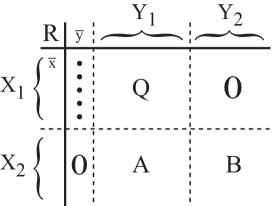
Figure 59: Relation $R$ decomposed into blocks for the proof of Lemma 64, as described below.

Specifically, pick some ${\overline{y}}\in Y$ such that $({\overline{x}},{\overline{y}})\in R$. This is possible since $R$ has no blank rows. Then decompose $X=X_{1}\cup X_{2}$, with $X_{1}=X_{\overline{y}}$ and $X_{2}=X\setminus{X_{1}}$. Since $R$ preserves attribute privacy, $X_{2}\neq\emptyset$.

Let $Q$ model $\mathop{\rm Lk}(\Phi_{R},{\overline{y}})$. So $Q$ is $R$ restricted to $X_{1}\times Y_{1}$, with $Y_{1}=\bigcup_{x\in{X_{1}}}Y_{x}\setminus\{{\overline{y}}\}$. If $Y_{1}\neq\emptyset$, then $Q$ preserves attribute privacy, by Lemma 57, and $Q$ has no blank columns.

Now write $Y$ as the disjoint union $Y=\{{\overline{y}}\}\cup Y_{1}\cup Y_{2}$, with $Y_{2}=Y\setminus(Y_{1}\cup\{{\overline{y}}\})$.

  

Observe that no individual in $X_{2}$ has attribute ${\overline{y}}$. Observe further that every individual in $X_{1}$ has attribute ${\overline{y}}$ but has no attributes in $Y_{2}$, by construction.

Let $A$ be the restriction of $R$ to $X_{2}\times Y_{1}$ and let $B$ be the restriction of $R$ to $X_{2}\times Y_{2}$.

If $Y_{2}\neq\emptyset$, then $B$ has no blank columns and $\Phi_{B}=\mathop{\rm dl}(\Phi_{R},Y_{1}\cup\{{\overline{y}}\})$. If $\lvert Y_{2}\rvert\geq 2$, then the blank rows indexed by $X_{1}$ that remain after deleting from $R$ the columns indexed by $Y_{1}\cup\{{\overline{y}}\}$ are irrelevant and so $B$ preserves attribute privacy (by Lemma 57 and by an argument similar to that appearing in the proof of the Subclaim on page C.3).

Let us look at some cases:

• $\lvert Y_{2}\rvert\geq\lvert X_{2}\rvert=1$:  Then any attribute of $Y_{2}$ identifies the one individual in $X_{2}$. Since $R$ preserves attribute privacy, this implies both that $\lvert Y_{2}\rvert=1$ and that relation $A$ is blank. Consequently, every attribute in $Y_{1}$ implies ${\overline{y}}$ in $R$. Since $R$ preserves attribute privacy, we conclude that $Y_{1}=\emptyset$. That means we are actually in the base case, with $n=2$.

• $\lvert Y_{2}\rvert>\lvert X_{2}\rvert\geq 2$:  By removing some columns of $B$, we obtain a square relation to which we can apply the induction hypothesis. That means every $x\in{X_{2}}$ is uniquely identifiable by the remaining columns. Since $B$ preserves attribute privacy that means the columns removed must have been blank, a contradiction.

• $\lvert Y_{2}\rvert=\lvert X_{2}\rvert\geq 2$:  We can apply the induction hypothesis directly to $B$. That again tells us that every $x\in{X_{2}}$ is uniquely identifiable by $Y_{2}\,$-indexed columns, both in $B$ and in $R$. We conclude that relation $A$ must be blank and so $Y_{1}=\emptyset$, arguing as above. Thus $\lvert X_{2}\rvert=\lvert Y_{2}\rvert=n-1$, implying $\lvert X_{1}\rvert=1$. So ${\overline{y}}$ uniquely identifies ${\overline{x}}$, as desired.

• $\lvert Y_{2}\rvert<\lvert X_{2}\rvert$:  This means $\lvert Y_{1}\rvert\geq\lvert X_{1}\rvert$. Additionally, $\lvert X_{1}\rvert\geq 2$, as otherwise ${\overline{y}}$ implies all the attributes $Y_{1}$. If actually $\lvert Y_{1}\rvert>\lvert X_{1}\rvert$, then we could argue as above to see that some columns of $Q$ are blank, contrary to the construction of $Q$. So we have that $n>\lvert Y_{1}\rvert=\lvert X_{1}\rvert\geq 2$ and the induction hypothesis applies. Consequently, ${\overline{x}}$ is uniquely identifiable via $Q$, say as $\{{\overline{x}}\}=\psi_{Q}(\gamma)$, for some $\gamma\subseteq Y_{1}$. If we adjoin ${\overline{y}}$, we get that $\psi_{R}(\gamma\cup\{{\overline{y}}\})=\psi_{Q}(\gamma)=\{{\overline{x}}\}$, as desired.

∎

Theorem 65 (Too Many Attributes).

Let $R$ be a relation on $\mskip 1.0mu{X}\mskip-1.8mu\times{Y}\mskip-2.0mu$ with no blank columns.

Suppose $\lvert Y\rvert>\lvert X\rvert\geq 1$.  Then $R$ does not preserve attribute privacy.

Proof.

The proof is a corollary to Lemma 64:

If $\lvert Y\rvert>\lvert X\rvert=1$, then all attributes in $\mskip 1.0mu{}Y\mskip-1.6mu$ are inferable from nothing (in the context of $R$).

Otherwise, suppose $R$ preserves attribute privacy. We have $\lvert Y\rvert>\lvert X\rvert>1$, so we can delete some columns of $R$ and apply Lemmas 57 and 64 to a resulting square relation. Every individual in $X$ is therefore uniquely identifiable via the columns retained. Consequently, either there is attribute inference in $R$ or the discarded columns were blank, a contradiction. ∎

Comment: One implication of this result and those in Appendix E is the old detective show mantra “eliminate suspects”: Reduce the number of relevant individuals sufficiently, and some attribute inference is assured. This amounts to moving from relation $R$ to a subrelation $Q$ representing $\mathop{\rm dl}(\Psi_{R},\sigma)$, with $\sigma$ a set  of “eliminated suspects”.

An additional conclusion: The proof of Lemma 64 suggests that perhaps $R$ also preserves association privacy. Indeed, we will see that to be true in Appendix E.4.

Appendix D Inference Hardness

Recall the following definition:

Definition 9 (Individual Privacy).

Let $R$ be a relation on ${X}\mskip-1.8mu\times{Y}$ and suppose $x\in X$.

We say that $R$ preserves attribute privacy for $x$ whenever $(\phi_{R}\circ\psi_{R})(\gamma)=\gamma$ for all $\gamma\subseteq Y_{x}$.

We have seen the following basic result within the proofs of other lemmas:

Lemma 66.

Let $R$ be a relation on ${X}\mskip-1.8mu\times{Y}$, with both $\hbox{\hskip 0.2pt}{}X\!$ and $\hbox{\hskip 1.0pt}{}Y\!$ nonempty. Let $x\in X$. Then:

$R$ preserves attribute privacy for $x$

if and only if

$(\phi_{R}\circ\psi_{R})(\gamma)=\gamma$, for all $\gamma$ of the form $\gamma=Y_{x}\setminus\{y\}$, with $y\in Y_{x}$.

Proof.

I. If $R$ preserves attribute privacy for $x$, then the condition is satisfied by definition.

II. Suppose $R$ does not preserve attribute privacy for $x$. Then for some $\gamma\subseteq Y_{x}$, $\gamma\subsetneq(\phi_{R}\circ\psi_{R})(\gamma)$. We know $(\phi_{R}\circ\psi_{R})(Y_{x})=Y_{x}$ by Corollary 47 on page 47, so by Lemma 48 on page 48 we can assume that $\gamma=Y_{x}\setminus\{y\}$, for some $y\in Y_{x}$. ∎

Lemma 66 tells us that it is fairly easy to check whether an individual’s attribute privacy is preserved. One merely needs to check whether any one attribute is implied by all the remaining attributes. That may be done quickly since the maps $\phi_{R}$ and $\psi_{R}$ amount to set intersections. Harder is finding a smallest set of attributes that implies another of the individual’s attributes.

Influenced by Lemma 60 on page 60, we formulate the following problem:

Definition 67 (Minimal Inference).

MinInf is the following decision problem:

Given relation $R$ on ${X}\mskip-1.8mu\times{Y}$, $x\in X$, $y\in Y$, and $k\geq 0$, is there a simplex $\gamma\in\Phi_{R}$, with $\gamma\,\subseteq Y_{x}\setminus\{y\}$, such that $\lvert\gamma\rvert\leq k$ and $\psi_{R}(\gamma)\subseteq\psi_{R}(\{y\})$?

Lemma 68.

MinInf is $N\!P$-complete

Proof.

(A) Observe that the problem lies in $N\!P$: Given some $\gamma$, one can verify the stated conditions in polynomial time. The verifications amount to set intersection, cardinality, and subset computations, drawn from the columns and one row of $R$.

(B) We will establish $N\!P$-hardness by a reduction from Set Cover. Recall: Given a collection of sets $\{S_{1},\ldots,S_{m}\}$, Set Cover asks whether there is some subcollection of size at most $k$ such that the union of the subcollection is the overall union (often called the universe).

Given an instance of the Set Cover problem, we define the following relation:

• $X\;=\;\{x_{0}\}\;\cup\;\bigcup_{i=1}^{m}S_{i}$, with $x_{0}$ a new element distinct from any elements in the sets $S_{i}$.

• $Y\;=\;\{0,1,\ldots,m\}$.

• $R\;\;=\big{(}\{x_{0}\}\times Y\big{)}\;\cup\;\bigcup_{i=1}^{m}{\big{\{}(x,i)\in{X}\mskip-1.8mu\times{Y}\;\left|\;x\in X\setminus{S_{i}}\right.\big{\}}}.$

In words: The $0^{\hbox{\footnotesize th}}$ column of $R$ is the singleton set $\{x_{0}\}$ and the $i^{\hbox{\footnotesize th}}$ column of $R$, for $i=1,\ldots,m$, is $X\setminus{S_{i}}$, i.e., the complement of $S_{i}$ in the original set cover universe, but now with $x_{0}$ added. The row for $x_{0}$ has entries for all possible attributes. All other rows have no entry in column 0.

Reduction: Given an instance of Set Cover, we transform it into an instance of MinInf using the relation $R$ given above and by letting $x=x_{0}$ and $y=0$. The parameter $k$ is the same for both problems. Observe that $Y_{x}\setminus\{y\}=\{1,\ldots,m\}$.

Observe further that $\lvert X\rvert=\lvert\bigcup_{i=1}^{m}S_{i}\rvert+1=n+1$ and $\lvert Y\rvert=m+1$, with $n$ the number of elements in the set cover universe and $m$ the number of subsets specified for the set cover problem. The reduction can therefore be computed in polynomial time.

To avoid trivialities, we assume that $n>0$ and $m>0$.

To complete the proof, we will establish the following:

Claim: The answer to Set Cover is “yes” if and only if the answer to MinInf is “yes”.

I. A “yes” answer to Set Cover means that there is some set of indices $\gamma\subseteq\{1,\ldots,m\}$, with $\lvert\gamma\rvert\leq k$, such that $\bigcup_{j\in\gamma}S_{j}=\bigcup_{i=1}^{m}S_{i}$. Therefore, since $0\not\in\gamma$,

$$\psi_{R}(\gamma)=\bigcap_{j\in\gamma}X_{j}=\bigcap_{j\in\gamma}(X\setminus{S_{j}})=X\setminus(\bigcup_{j\in\gamma}S_{j})=X\setminus(\bigcup_{i=1}^{m}S_{i})=\{x_{0}\}=\psi_{R}(\{0\})=\psi_{R}(\{y\}).$$

Consequently, $\emptyset\neq\psi_{R}(\gamma)\subseteq\psi_{R}(\{y\})$ with $\gamma\subseteq{Y_{x}\setminus\{y\}}$ and $\lvert\gamma\rvert\leq k$, meaning that the answer to MinInf is “yes” as well.

II. A “yes” answer to MinInf means there is some $\gamma\subseteq\{1,\ldots,m\}$ such that $\lvert\gamma\rvert\leq k$ and $\emptyset\neq\psi_{R}(\gamma)\subseteq\psi_{R}(\{y\})$.  Observe that $\psi_{R}(\{y\})=\psi_{R}(\{0\})=\{x_{0}\}$ and that

$$\psi_{R}(\gamma)\;=\;\bigcap_{j\in\gamma}X_{j}\;=\;\bigcap_{j\in\gamma}(X\setminus{S_{j}})\;=\;X\setminus(\bigcup_{j\in\gamma}S_{j}).$$

The middle equality holds as before because $0\not\in\gamma$.

So we see that $x_{0}\in X\setminus(\bigcup_{j\in\gamma}S_{j})\subseteq\{x_{0}\}$, telling us

$$\bigcup_{j\in\gamma}S_{j}\;=\;X\setminus\{x_{0}\}\;=\;\bigcup_{i=1}^{m}S_{i}.$$

That means $\gamma$ describes a set of indices sought for by Set Cover, with $\lvert\gamma\rvert\leq k$, so the answer to Set Cover is also “yes”. ∎

Appendix E Privacy Spheres

The aim of this appendix is to characterize privacy and inference in terms of spheres. Spheres exhibit homogeneity, which is good for privacy, while still admitting a coordinate system for identifiability.

We first prove a theorem characterizing individual attribute privacy, then a generalization that holds for arbitrary elements of a relation’s doubly-labeled poset, and finally a characterization of those relations that preserve both attribute and association privacy.

E.1 Individual Attribute Privacy

We first state a lemma as a tool. Recall also Definitions 6 and 9 (see pages C.3 and D).

Lemma 69.

Let $R$ be a relation on ${X}\mskip-1.8mu\times{Y}$, with both $\hbox{\hskip 1.0pt}{}X\!$ and $\hbox{\hskip 1.0pt}{}Y\!$ nonempty.
Let $x\in X$ be uniquely identifiable via $R$.  Then:

$$\Big{(}\bigcap_{y\in Y_{x}}X_{y}\Big{)}\setminus\{x\}\;=\;\emptyset.$$

Moreover, $R$ preserves attribute privacy for $x$ if and only if

$$\Big{(}\bigcap_{y\in\gamma}X_{y}\Big{)}\setminus\{x\}\;\neq\;\emptyset,\quad\hbox{for all $\;\gamma\subsetneq Y_{x}$}.$$

Proof.

The first statement follows from the definition of unique identifiability: $\bigcap_{y\in Y_{x}}X_{y}=\psi_{R}(Y_{x})=\{x\}$.

For the second statement:

I. Assume that $R$ preserves attribute privacy for $x$. Let $\gamma\subsetneq{Y_{x}}$. If $\big{(}\bigcap_{y\in\gamma}X_{y}\big{)}\setminus\{x\}=\emptyset$, then $\psi_{R}(\gamma)=\bigcap_{y\in\gamma}X_{y}=\{x\}$, since $x\in{X_{y}}$ whenever $y\in\gamma\subseteq{Y_{x}}$ (when $\gamma=\emptyset$, the vacuous intersection is all of $X$, containing $x$). That says a proper subset of $Y_{x}$ identifies $x$, contradicting the proof of Lemma 61 on page 61.

II. Assume $\big{(}\bigcap_{y\in\gamma}X_{y}\big{)}\setminus\{x\}\neq\emptyset$ for all proper subsets $\gamma$ of $Y_{x}$. If $R$ fails to preserve attribute privacy for $x$, then by Lemma 66 on page 66 there is some $\gamma$ of the form $Y_{x}\setminus\{y\}$, with $y\in{Y_{x}}$, such that $\gamma\subsetneq(\phi_{R}\circ\psi_{R})(\gamma)=Y_{x}$. Applying $\psi_{R}$ to both sides of that last equality gives $\psi_{R}(\gamma)=\psi_{R}(Y_{x})=\{x\}$, by unique identifiability. That is a contradiction, since $\psi_{R}(\gamma)=\bigcap_{y\in\gamma}X_{y}$. ∎

We now address our characterization of individual privacy, proving a theorem stated previously:

Theorem 10 (Individual Attribute Privacy).

Let $R$ be a relation on ${X}\mskip-1.8mu\times{Y}$, with $\lvert X\rvert>1$. Suppose $x\in X$ is uniquely identifiable via $R$.  Let $Q$ be the relation modeling $\mathop{\rm Lk}(\Psi_{R},x)$.
Then the following three conditions are equivalent:

1. $R$ preserves attribute privacy for $x$.

2. $\mathop{\rm Lk}(\Psi_{R},x)\;\simeq\;\,\mathbb{S}^{\kern 0.56001pt{k-2}}$, with $k=\lvert Y_{x}\rvert$.

3. $\Phi_{Q}\;=\;\partial(Y_{x})$.

Proof.

The hypotheses ensure that $Y_{x}\neq\emptyset$ (and so also $Y\!\neq\emptyset$). They also ensure that $x$ is a vertex of $\Psi_{R}$, so the link is not void. It could be an empty complex $\{\emptyset\}$, of course.

Observe that $Q$ is the restriction of $R$ to $\overline{X}\times Y_{x}$, with $\overline{X}=\bigcup_{y\in Y_{x}}X_{y}\setminus\{x\}$.

If $\overline{X}=\emptyset$, then, reasoning as in the proof of Lemma 55 on page 55, we see that $\mathop{\rm Lk}(\Psi_{R},x)=\{\emptyset\}=\mathbb{S}^{\kern 0.56001pt{-1}}$. Furthermore, $x$ does not share any of its attributes with any other individuals in $X$. By convention, $\Phi_{Q}=\{\emptyset\}$ as well. If $k=\lvert Y_{x}\rvert=1$, meaning $x$ has a single attribute, then $R$ preserves attribute privacy for $x$, since $\lvert X\rvert>1$. Also, $\mathbb{S}^{\kern 0.56001pt{k-2}}=\mathbb{S}^{\kern 0.56001pt{-1}}=\{\emptyset\}=\partial(Y_{x})$. So conditions (a), (b), (c) all hold. If $k=\lvert Y_{x}\rvert\geq 2$, then any one attribute of $Y_{x}$ implies all the others, so condition (a) does not hold. Moreover, conditions (b) and (c) also do not hold. In short, the theorem holds when $\overline{X}=\emptyset$.

We now assume that $\overline{X}\neq\emptyset$. We then know that $\mathop{\rm Lk}(\Psi_{R},x)=\Psi_{Q}\simeq\Phi_{Q}$ by a dual version of Lemma 55 and by Dowker duality. Definitionally, $\partial(Y_{x})\simeq\mathbb{S}^{\kern 0.56001pt{k-2}}$, with $k=\lvert Y_{x}\rvert>0$. We therefore see that (c) implies (b). To see that (b) implies (c), observe that the underlying vertex set of $\Phi_{Q}$ is $Y_{x}$, so $\Phi_{Q}\simeq\mathbb{S}^{\kern 0.56001pt{k-2}}$ means $\Phi_{Q}=\partial(Y_{x})$, since no proper subset of a sphere can be homotopic to that same sphere. To prove the theorem we therefore only need to establish that conditions (a) and (c) are equivalent.

Recall the formulas relating $\phi_{Q}$ and $\phi_{R}$ from page • ‣ C.1 and dualize them here. We see that:

$$\psi_{Q}(\chi)\;=\;\psi_{R}(\chi)\setminus\{x\}\;=\;\Big{(}\bigcap_{y\in\chi}X_{y}\Big{)}\setminus\{x\},\quad\hbox{for all $\emptyset\neq\chi\subseteq{Y_{x}}$}.$$

I. Assume that $R$ preserves attribute privacy for $x$. By Lemma 69 and the formula above we see that $\psi_{Q}(\chi)\neq\emptyset$ for all nonempty proper subsets $\chi$ of $Y_{x}$ and that $\psi_{Q}(Y_{x})=\emptyset$, since $x$ is uniquely identifiable via $R$. Consequently, $\Phi_{Q}$ contains every nonempty proper subset of $Y_{x}$ as a simplex, but does not contain $Y_{x}$. (Also, $\Phi_{Q}$ contains the empty simplex since the complex is not void.) Thus $\Phi_{Q}=\partial(Y_{x})$.

II. Assume that $\Phi_{Q}=\partial(Y_{x})$. Then $\psi_{Q}(\chi)\neq\emptyset$ for every nonempty proper subset $\chi$ of $Y_{x}$. By the formula above, $\big{(}\bigcap_{y\in\chi}X_{y}\big{)}\setminus\{x\}\;\neq\;\emptyset$, for each such $\chi$. Now suppose $\chi=\emptyset\subsetneq{Y_{x}}$. Then:

$$\emptyset\;\neq\;\overline{X}\;=\;\psi_{Q}(\emptyset)\;\subseteq\;X\setminus\{x\}\;=\;\Big{(}\bigcap_{y\in\emptyset}X_{y}\Big{)}\setminus\{x\}.$$

So we see that $\;\big{(}\bigcap_{y\in\chi}X_{y}\big{)}\setminus\{x\}\;\neq\;\emptyset\;$ for every proper subset $\chi$ of $Y_{x}$, implying that $R$ preserves attribute privacy for $x$, by Lemma 69. ∎

Comment: It is impossible to satisfy the following three conditions simultaneously:

(1) $x$ is uniquely identifiable, (2) $\lvert Y_{x}\rvert=1$, (3) $\overline{X}\neq\emptyset$.

E.2 Group Attribute Privacy

We now generalize the previous theorem to arbitrary elements $(\sigma,\gamma)$ of the doubly-labeled poset $P_{R}$ associated with a relation $R$. We stated the generalized theorem previously in the report, as Theorem 11, and replicate that below. One may view this generalized theorem as a characterization of the conditions under which a set $\sigma$ of individuals (i.e., a group of individuals, in the non-mathematical sense) has its attribute privacy preserved, as a whole, not necessarily individually.  Theorem 10 is a special case of Theorem 11, with the “group” a single individual $x$, since $(\{x\},Y_{x})\in P_{R}$ whenever $x$ is uniquely identifiable via $R$ and $Y_{x}\neq\emptyset$.

Theorem 11 (Group Attribute Privacy).

Let $R$ be a relation on ${X}\mskip-1.8mu\times{Y}$.
Suppose $(\sigma,\gamma)\in P_{R}$, with $\sigma\neq X$.  Let $Q$ be the relation modeling $\mathop{\rm Lk}(\Psi_{R},\sigma)$.
Then the following three conditions are equivalent:

1. $(\phi_{R}\circ\psi_{R})(\gamma^{\prime})\;=\;\gamma^{\prime}$, for every subset $\gamma^{\prime}$ of $\gamma$.

2. $\mathop{\rm Lk}(\Psi_{R},\sigma)\;\simeq\;\mathbb{S}^{\kern 0.56001pt{k-2}}$, with $k=\lvert\gamma\rvert$.

3. $\Phi_{Q}\;=\;\partial(\gamma)$.

Proof.

Reminder: Since $(\sigma,\gamma)\in P_{R}$,  $\emptyset\neq\sigma\in\Psi_{R}$, $\,\emptyset\neq\gamma\in\Phi_{R}$, $\,\phi_{R}(\sigma)=\gamma$, and $\psi_{R}(\gamma)=\sigma$.

Thus also $(\phi_{R}\circ\psi_{R})(\gamma)=\gamma$, meaning we can focus on proper subsets of $\gamma$ for part (a).

Recall also that $Q$ is the restriction of $R$ to $\overline{X}\times\gamma$, with $\overline{X}=\bigcup_{y\in\gamma}X_{y}\setminus\sigma$.

If $\overline{X}=\emptyset$, then $\mathop{\rm Lk}(\Psi_{R},\sigma)=\{\emptyset\}=\mathbb{S}^{\kern 0.56001pt{-1}}$. By convention, $\Phi_{Q}=\{\emptyset\}$ as well. If $k=\lvert\gamma\rvert=1$, then $\mathbb{S}^{\kern 0.56001pt{k-2}}=\mathbb{S}^{\kern 0.56001pt{-1}}=\{\emptyset\}=\partial(\gamma)$. The only proper subset of $\gamma$ in this case is $\gamma^{\prime}=\emptyset$, and $(\phi_{R}\circ\psi_{R})(\emptyset)=\phi_{R}(X)=\emptyset$. (Reason: If $y\in\phi_{R}(X)$, then $y\in\gamma$, so $\gamma=\{y\}$, implying $\sigma=X$, which is disallowed.) Thus conditions (a), (b), (c) all hold. If $k=\lvert\gamma\rvert\geq 2$, then conditions (b) and (c) cannot hold. Also, condition (a) does not hold since $(\phi_{R}\circ\psi_{R})(\{y\})=\gamma$ for each $y\in\gamma$, bearing in mind that $\overline{X}=\emptyset$ means $X_{y}=\sigma$ for each $y\in\gamma$. In short, the theorem holds when $\overline{X}=\emptyset$.

We now assume that $\overline{X}\neq\emptyset$. As in the proof of Theorem 10, we see readily that conditions (b) and (c) are equivalent, so we will prove that conditions (a) and (c) are equivalent. And, as in the previous proof, dualizing a formula from page • ‣ C.1 gives this formula:

$$\psi_{Q}(\chi)\;=\;\psi_{R}(\chi)\setminus\sigma,\quad\hbox{for all $\emptyset\neq\chi\subseteq{\gamma}$}.$$

• Assume that $(\phi_{R}\circ\psi_{R})(\gamma^{\prime})\;=\;\gamma^{\prime}$, for every subset $\gamma^{\prime}$ of $\gamma$.
  We will establish that $\Phi_{Q}$ contains all proper subsets of $\gamma$ but not $\gamma$, telling us $\Phi_{Q}=\partial(\gamma)$.

  Since $\Phi_{Q}$ is not void, it contains the empty simplex.

  Pick some $\emptyset\neq\gamma^{\prime}\subsetneq\gamma$.  Since $(\phi_{R}\circ\psi_{R})(\gamma^{\prime})\;=\;\gamma^{\prime}$, $\psi_{R}(\gamma^{\prime})\supsetneq\sigma$.

  The formula above therefore says $\psi_{Q}(\gamma^{\prime})\neq\emptyset$, telling us $\gamma^{\prime}\in\Phi_{Q}$.

  Similarly, $\psi_{Q}(\gamma)\;=\;\psi_{R}(\gamma)\setminus\sigma\;=\;\sigma\setminus\sigma\;=\;\emptyset$, so $\gamma\not\in\Phi_{Q}$.

• Assume that $\Phi_{Q}=\partial(\gamma)$.

  Recall that $k=\lvert\gamma\rvert>0$. We look at two cases based on the value of $k$:

  • In this case, $\gamma=\{y\}$, for some $y\in Y$, so $\sigma=X_{y}$ and $\overline{X}=\emptyset$, which we discussed above.

  • Suppose, for the sake of contradiction, that $\gamma^{\prime}\subsetneq(\phi_{R}\circ\psi_{R})(\gamma^{\prime})$, for some $\gamma^{\prime}\subsetneq\gamma$. By Lemma 48 on page 48, we can assume $\gamma^{\prime}=\gamma\setminus\{y\}$, for some $y\in\gamma$. Consequently, $(\phi_{R}\circ\psi_{R})(\gamma^{\prime})=\gamma$, which implies $\psi_{R}(\gamma^{\prime})=\sigma$. The formula on the previous page then says $\psi_{Q}(\gamma^{\prime})=\emptyset$, whereas $\gamma^{\prime}\in\Phi_{Q}$ means $\psi_{Q}(\gamma^{\prime})\neq\emptyset$, a contradiction.

∎

  

The following lemma, previously stated on page 12, relates privacy preservation in a link to privacy preservation in the encompassing relation.

Lemma 12 (Interpreting Local Operators).

Let $R$ be a relation on ${X}\mskip-1.8mu\times{Y}$.

Suppose $(\sigma,\gamma)\in P_{R}$, with $\sigma\neq X$.

Let $Q$ be the relation on $\overline{X}\times\gamma$ that models $\mathop{\rm Lk}(\Psi_{R},\sigma)$ and suppose $\overline{X}\neq\emptyset$.  

Then, for every $\gamma^{\prime}\subseteq\gamma$:

1. If $\,\gamma^{\prime}\not\in\Phi_{Q}$, then $\psi_{R}(\gamma^{\prime})=\sigma$.

2. If $\,\gamma^{\prime}\in\Phi_{Q}$, then $\psi_{R}(\gamma^{\prime})\supsetneq\sigma$.

   Moreover, in this case:

   For $\,\gamma^{\prime}=\emptyset$,  $(\phi_{Q}\circ\psi_{Q})(\emptyset)\supseteq(\phi_{R}\circ\psi_{R})(\emptyset)$.

   If $\,\gamma^{\prime}\neq\emptyset$,  then $(\phi_{Q}\circ\psi_{Q})(\gamma^{\prime})=(\phi_{R}\circ\psi_{R})(\gamma^{\prime})$.

Proof.

Observe that for every $\gamma^{\prime}\subseteq\gamma$, one has $\gamma^{\prime}\in\Phi_{R}$ and $\psi_{R}(\gamma^{\prime})\supseteq\psi_{R}(\gamma)=\sigma$.

By formulas from page • ‣ C.1 dualized,  $\psi_{Q}(\gamma^{\prime})=\psi_{R}(\gamma^{\prime})\setminus\sigma$  and  $\psi_{R}(\gamma^{\prime})=\psi_{Q}(\gamma^{\prime})\cup\sigma$, when $\emptyset\neq\gamma^{\prime}\subseteq\gamma$.

(i) Suppose $\gamma^{\prime}\not\in\Phi_{Q}$. Then $\gamma^{\prime}\neq\emptyset$, since $\emptyset\in\Phi_{Q}$. Also, $\psi_{Q}(\gamma^{\prime})=\emptyset$, so by the second formula above, $\psi_{R}(\gamma^{\prime})=\sigma$.

(ii) Suppose $\gamma^{\prime}\in\Phi_{Q}$. If $\gamma^{\prime}=\emptyset$, then $\psi_{R}(\emptyset)=X\supsetneq\sigma$, by hypothesis. If $\gamma^{\prime}\neq\emptyset$, then $\psi_{Q}(\gamma^{\prime})\neq\emptyset$, so by the formulas above, $\psi_{R}(\gamma^{\prime})\supsetneq\sigma$.

Turning to the “Moreover”:

If $y\in(\phi_{R}\circ\psi_{R})(\emptyset)$, then $y$ is an attribute for all individuals in $X$, so $y\in\gamma$ and $y\in\phi_{Q}(\overline{X})=(\phi_{Q}\circ\psi_{Q})(\emptyset)$.

Let $\emptyset\neq\gamma^{\prime}\!\in\Phi_{Q}$. By another formula on page • ‣ C.1 dualized, if $\kappa\subseteq\overline{X}$, then $\phi_{Q}(\kappa)=\phi_{R}(\kappa\cup\sigma)$.

Therefore, using the first formula above: $(\phi_{Q}\circ\psi_{Q})(\gamma^{\prime})=\phi_{Q}(\psi_{R}(\gamma^{\prime})\setminus\sigma)=(\phi_{R}\circ\psi_{R})(\gamma^{\prime})$. ∎

Comment:  Also, $(\phi_{Q}\circ\psi_{Q})(\emptyset)=\phi_{Q}(\overline{X})=\phi_{R}\big{(}\bigcup_{y\in\gamma}X_{y}\,\big{)}=\bigcap_{y\in\gamma}(\phi_{R}\circ\psi_{R})(\{y\})$.

E.3 Preserving Attribute and Association Privacy

In this subsection, we are interested in understanding relations that preserve  both  attribute and association privacy. We will discover that this requirement is severely limiting. As we already see from Theorem 65 on page 65, if $R$ is a nonvoid tight relation on ${X}\mskip-1.8mu\times{Y}$ that preserves both attribute and association privacy, then $\lvert X\rvert=\lvert Y\rvert=n$.  What are the possibilities?

• Not relevant; this is a void relation.

• Not possible; such a relation does not preserve privacy; one can infer the single individual or single attribute “for free” (e.g., merely by knowing someone is covered by the relation).

• As we have seen before, such a relation must be isomorphic to the following relation:

  $$\begin{array}[]{c|cc}R&y_{1}&y_{2}\\[2.0pt] \hline\cr x_{1}&\bullet&\\ x_{2}&&\bullet\\ \end{array}$$

  Then both $\Psi_{R}$ and $\Phi_{R}$ are instances of the 0-sphere $\mathbb{S}^{\kern 0.56001pt{0}}$.

• Now there are several possibilities:

  • The relation could be isomorphic to a cyclic staircase relation:

    $$\begin{array}[]{c|cccccc}R&y_{1}&y_{2}&\cdots&\cdots&y_{n-1}&y_{n}\\[2.0pt] \hline\cr x_{1}&\bullet&\bullet&&&&\\ x_{2}&&\bullet&\bullet&&&\\ \vdots&&&\ddots&\ddots&&\\ \vdots&&&&\ddots&\bullet&\\ x_{n-1}&&&&&\bullet&\bullet\\ x_{n}&\bullet&&&&&\bullet\\ \end{array}$$

    Then both $\Psi_{R}$ and $\Phi_{R}$ are homotopic to the 1-sphere $\mathbb{S}^{1}$. Each is simply a linear cycle of edges, with vertices in one complex dualizing to edges in the other.

  • The relation could be isomorphic to a spherical boundary relation, in which every entry is present except that a diagonal is blank. For example, in the following relation all entries are present except those of the form $(x_{i},y_{n-i+1})$, $i=1,\ldots,n$:

    $$\begin{array}[]{c|cccccc}R&y_{1}&y_{2}&\cdots&\cdots&y_{n-1}&y_{n}\\[2.0pt] \hline\cr x_{1}&\bullet&\bullet&\bullet&\cdots&\bullet&\\ x_{2}&\bullet&\bullet&\cdots&\bullet&&\bullet\\ \vdots&\vdots&\vdots&\mkern 1.0mu\raise 1.0pt\vbox{\kern 7.0pt\hbox{.}}\mkern 2.0mu\raise 4.0pt\hbox{.}\mkern 2.0mu\raise 7.0pt\hbox{.}&&\bullet&\vdots\\ \vdots&\bullet&\bullet&&\mkern 1.0mu\raise 1.0pt\vbox{\kern 7.0pt\hbox{.}}\mkern 2.0mu\raise 4.0pt\hbox{.}\mkern 2.0mu\raise 7.0pt\hbox{.}&\vdots&\bullet\\ x_{n-1}&\bullet&&\bullet&\cdots&\bullet&\bullet\\ x_{n}&&\bullet&\bullet&\cdots&\bullet&\bullet\\ \end{array}$$

    Then $\Psi_{R}$ and $\Phi_{R}$ are each boundary complexes, namely $\Psi_{R}=\partial(X)$ and $\Phi_{R}=\partial(Y)$. Thus both are homotopic to the $(n-2)$-sphere $\mathbb{S}^{\kern 0.56001pt{n-2}}$.

  • Finally, $R$ could have multiple components, each of which is isomorphic to one of the following: A singleton, a cyclic staircase relation, or a spherical boundary relation, all as above. (Observe that even though a nonblank $1\times 1$ relation in and of itself preserves no privacy, a relation containing a nonblank $1\times 1$ subrelation can preserve privacy when that subrelation is one of several components.)

  (Comment: the staircase and spherical relations are isomorphic when $n=3$.)

The aim of this subsection is to prove that these are the only possibilities.

Lemma 70.

Let $R$ be a connected tight relation on ${X}\mskip-1.8mu\times{Y}$, with $\lvert X\rvert=\lvert Y\rvert\geq 3$, that preserves both attribute and association privacy.

Let $x\in X$ and define $Q$ to be the relation on $\overline{X}\times Y_{x}$ that models $\mathop{\rm Lk}(\Psi_{R},x)$.

Then $\Psi_{Q}=\partial(\overline{X})$ and  $\Phi_{Q}=\partial(Y_{x})$, with $\lvert\overline{X}\rvert=\lvert Y_{x}\rvert$.

Proof.

Observe that $Y_{x}\neq\emptyset$ since $R$ is tight. Recall that $\overline{X}=\bigcup_{y\in Y_{x}}X_{y}\setminus\{x\}$, which is nonempty since $R$ is connected and $X$ contains not just $x$.

By Lemma 64 on page 64, $x$ is uniquely identifiable via $R$, so Theorem 10 on page 69 says that $\Psi_{Q}\simeq\mathbb{S}^{\kern 0.56001pt{k-2}}$ and $\Phi_{Q}=\partial(Y_{x})$, with $k=\lvert Y_{x}\rvert$. If we can show that $\lvert\overline{X}\rvert=k$, then we can conclude that $\Psi_{Q}=\partial(\overline{X})$.     (We also see that $k\geq 2$, since $\overline{X}\neq\emptyset$.)

The vertices of $\Psi_{Q}$ generate the maximal simplices of $\Phi_{Q}$. In particular, there exist distinct $x_{1},\ldots,x_{k}\in\overline{X}$ such that $\overline{Y}_{\!1},\ldots,\overline{Y}_{\!k}$ are the maximal simplices of $\Phi_{Q}$, with $\overline{Y}_{\!i}=Y_{x_{\scriptstyle i}}\cap Y_{x}$, and $\lvert\overline{Y}_{\!i}\rvert=k-1$, for $i=1,\ldots,k$.

Let ${\tilde{x}}\in\overline{X}$. Then $Y_{\tilde{x}}\cap Y_{x}\subseteq\overline{Y}_{\!i}\subseteq Y_{x_{\scriptstyle i}}$, for some $i\in\{1,\ldots,k\}$.

That says $\emptyset\neq\phi_{R}(\{{\tilde{x}},x\})\subseteq\phi_{R}(\{x_{i}\})$.

Since $R$ preserves association privacy, the dualization of Lemma 60 on page 60 implies ${\tilde{x}}=x_{i}$.  Thus $\lvert\overline{X}\rvert=k$. ∎

Comment: Where did we use the assumption that each of $X$ and $Y$ has at least three elements? In fact, for much of the proof it is enough to assume that $\lvert X\rvert=\lvert Y\rvert\geq 2$. However, there is no connected tight relation that preserves privacy when $\lvert X\rvert=\lvert Y\rvert=2$.

Corollary 71.

Let $R$ be a connected tight relation on ${X}\mskip-1.8mu\times{Y}$, with $\lvert X\rvert=\lvert Y\rvert$, that preserves both attribute and association privacy.

Let $y\in Y$ and suppose $\lvert X_{y}\rvert\geq 4$.

Then $\mathop{\rm Lk}(\Phi_{R},y)$ is not a linear cycle.  (In other words, the relation $Q$ that models $\mathop{\rm Lk}(\Phi_{R},y)$ is not isomorphic to a cyclic staircase relation.)

Proof.

Arguing as in the proof of Lemma 70, now in dual form, we see that $\mathop{\rm Lk}(\Phi_{R},y)\simeq\mathbb{S}^{\kern 0.56001pt{k-2}}$, with $k=\lvert X_{y}\rvert$.  Since $k-2\;\geq\;2$,  $\mathop{\rm Lk}(\Phi_{R},y)$ is not a linear cycle. ∎

Corollary 72.

Let $R$ be a connected tight relation on ${X}\mskip-1.8mu\times{Y}$, with $\lvert X\rvert=\lvert Y\rvert\geq 3$, that preserves both attribute and association privacy.

Suppose $\{x,x^{\prime}\}$, with $x\neq x^{\prime}$, is an edge (1-simplex) in $\Psi_{R}$.

Then $\lvert Y_{x}\rvert=\lvert Y_{x^{\prime}}\rvert$.

Proof.

Let $k=\lvert Y_{x}\rvert$ and $k^{\prime}=\lvert Y_{x^{\prime}}\rvert$.

Observe that $x^{\prime}$ is a vertex of $\mathop{\rm Lk}(\Psi_{R},x)$ and $x$ is a vertex of $\mathop{\rm Lk}(\Psi_{R},x^{\prime})$.

By the proof of Lemma 70, each of $x^{\prime}$ and $x$ generates a maximal simplex in the attribute complex associated with the other’s link. That simplex is ${Y_{x}\cap Y_{x^{\prime}}}$ in both complexes.

So $k-1=\lvert Y_{x}\cap Y_{x^{\prime}}\rvert=k^{\prime}-1$, hence $k=k^{\prime}$. ∎

Corollary 73.

Let $R$ be a connected tight relation on ${X}\mskip-1.8mu\times{Y}$, with $\lvert X\rvert=\lvert Y\rvert\geq 3$, that preserves both attribute and association privacy.

Then all rows and columns have the same number of nonblank entries.

Proof.

By Lemma 51 on page 51 and Corollary 72 above, all rows have the same number, $k_{r}$, of nonblank entries. Dualizing, one sees that all columns have the same number, $k_{c}$ , of nonblank entries. We claim that $k_{c}=k_{r}$. This assertion follows from Lemma 70 and its proof as follows:

Pick some $x\in X$ and let $Q$ be the relation modeling $\mathop{\rm Lk}(\Psi_{R},x)$. By Lemma 70, $\Psi_{Q}$ and $\Phi_{Q}$ are each boundary complexes, with $k_{r}=\lvert Y_{x}\rvert$ vertices. Moreover, each attribute $y\in Y_{x}$ generates a maximal simplex $X_{y}\cap\overline{X}$ in $\Psi_{Q}$, which must have size $k_{r}-1$. The column $X_{y}$ contains one additional individual, namely $x$.  So $k_{c}=\lvert X_{y}\rvert=(k_{r}-1)+1=k_{r}$. ∎

Theorem 74 (Privacy as Sphere).

Let $R$ be a nonvoid connected tight relation on $\hbox{\hskip 1.0pt}{}{X}\mskip-1.8mu\times{Y}\mskip-2.0mu$ that preserves both attribute and association privacy.

Then $\lvert X\rvert=\lvert Y\rvert\geq 3$ and $R$ is isomorphic to either a cyclic staircase relation or a spherical boundary relation (each described on page – ‣ $n\geq{3}$:).

Proof.

As we commented previously, Theorem 65 on page 65 implies that $\lvert X\rvert=\lvert Y\rvert=n$, for some $n\geq 2$. Connectedness further means that $n\geq 3$.

By Corollary 73, all rows and columns in $R$ have the same number of nonblank entries. In other words, $\lvert X_{y}\rvert=\lvert Y_{x}\rvert=k$, for all $x\in X$ and all $y\in Y$, for some fixed $k$. By connectedness, $k\geq 2$.

By Lemma 64 on page 64, each $x\in X$ is uniquely identifiable via $R$. Dualized, each $y\in Y$ is uniquely identifiable via $R$ as well.

If $k=2$, then $\Psi_{R}$ and $\Phi_{R}$ contain vertices and edges but no higher-dimensional simplices. By duality, each vertex therefore has at most two incident edges. By unique identifiability, each vertex has exactly two incident edges. Thus, by connectedness, each complex is a linear cycle. So $R$ is isomorphic to a cyclic staircase relation.

Now assume that $k\geq 3$.

Pick a ${\overline{y}}\in Y$ and consider the decomposition of Figure 60, similar to the one we saw in the proof of Lemma 64.

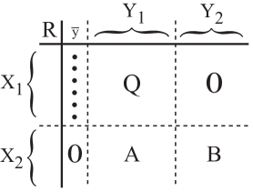
000000

Figure 60: Relation $R$ decomposed into blocks for the proof of Theorem 74.

Let $X_{1}=X_{\overline{y}}$ and write $X=X_{1}\cup X_{2}$ with $X_{2}=X\setminus{X_{1}}$. $X_{1}\neq\emptyset$ since every column of $R$ has $k$ nonblank entries and $X_{2}\neq\emptyset$ since $R$ preserves attribute privacy.

Let $Q$ model $\mathop{\rm Lk}(\Phi_{R},{\overline{y}})$. So $Q$ is $R$ restricted to $X_{1}\times Y_{1}$, with $Y_{1}=\bigcup_{x\in{X_{1}}}Y_{x}\setminus\{{\overline{y}}\}$. $Y_{1}\neq\emptyset$ because every row of $R$ has $k$ nonblank entries. In particular, there are exactly $k-1$ entries in each row of $Q$, so at least two entries in each row.

Now write $Y$ as the disjoint union $Y=\{{\overline{y}}\}\cup Y_{1}\cup Y_{2}$, with $Y_{2}=Y\setminus(Y_{1}\cup\{{\overline{y}}\})$. Observe that every individual in $X_{1}$ has attribute ${\overline{y}}$ but has no attributes in $Y_{2}$, by construction.

By the dual to Lemma 70, we know that $\Psi_{Q}=\partial(X_{1})$ and $\Phi_{Q}=\partial(Y_{1})$, with $k=\lvert X_{1}\rvert=\lvert Y_{1}\rvert$. Therefore, for each each $y\in Y_{1}$, column $X_{y}$ of $R$ has $k-1$ entries that lie in $X_{1}$ and one entry that lies in $X_{2}$. We claim that the $X_{2}$ entry is the same across all columns $X_{y}$ as $y$ varies over $Y_{1}$. For otherwise, at least two such columns would have an intersection (nonempty, since $k-2\geq 1$) contained wholly within $X_{\overline{y}}$, implying that $R$ permits attribute inference after all, by Lemma 60 on page 60. Call that common individual ${\overline{x}}$. Observe that $Y_{\overline{x}}=Y_{1}$ since every row of $R$ has exactly $k$ attributes. Consequently, the block diagram for $R$ becomes as in Figure 61.  (The figures now indicate blank entries either by blanks or by explicit “$0$”s.)

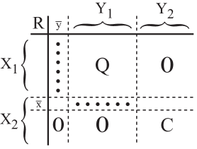
000000

Figure 61: Relation $R$ decomposed further.

Observe that no individual of $X_{1}\cup\{{\overline{x}}\}$ has any attributes in $Y_{2}$ and that no individual of $X_{2}\setminus\{{\overline{x}}\}$ has any attributes in $Y_{1}\cup\{{\overline{y}}\}$, by the row and column cardinality constraints. That means relation $C$, which is the restriction of $R$ to $(X_{2}\setminus\{{\overline{x}}\})\times Y_{2}$, would be disconnected from the rest of $R$, if $C$ were to exist. We conclude that $Y_{2}=\emptyset$ and that $X_{2}=\{{\overline{x}}\}$. Thus, finally, $R$ must decompose as in Figure 62. As we have seen, $Q$ is nearly a full relation, missing only a diagonal. We now see that $R$ is also nearly a full relation, missing only a diagonal. Thus $\Psi_{R}=\partial(X)$ and $\Phi_{R}=\partial(Y)$, meaning $R$ is isomorphic to a spherical boundary relation, as claimed.

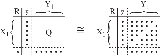
Figure 62: Relation $R$ decomposes diagonally.

∎

Corollary 75.

Let $R$ be a nonvoid tight relation that preserves both attribute and association privacy. Decompose $R$ into its connected components as $R=R_{1}\cup\cdots\cup R_{\ell}$, with each $\hbox{\hskip 1.0pt}{}R_{i}$ a nonvoid tight relation on $X_{i}\times Y_{i}$, as per the proof of Lemma 52 on page 52.  Then, for each $i\in\{1,\ldots,\ell\}$,  $R_{i}$ is isomorphic to a singleton or a cyclic staircase relation or a spherical boundary relation, and $\lvert X_{i}\rvert=\lvert Y_{i}\rvert$.

Comment: When $\ell=2$ and each of $R_{1}$ and $R_{2}$ is a singleton, then the Dowker complexes of $R$ itself, $\Psi_{R}$ and $\Phi_{R}$, are each an instance of $\mathbb{S}^{\kern 0.56001pt{0}}$.

Proof.

Consider $R_{i}$, for some $i\in\{1,\ldots,\ell\}$.

Suppose that $X_{i}\in\Psi_{R_{\scriptstyle i}}$. Then some attribute $y\in Y_{i}$ is shared by all individuals in $X_{i}$. If there were any other attributes in $Y_{i}$, then each of those would individually imply $y$ in $R$. Since $R$ preserves attribute privacy, $\lvert Y_{i}\rvert=1$. Consequently, since $R$ also preserves association privacy, $\lvert X_{i}\rvert=1$, so $R_{i}$ is a singleton.

If $R_{i}$ is not a singleton, then $X_{i}\not\in\Psi_{R_{\scriptstyle i}}$ and similarly $Y_{i}\not\in\Phi_{R_{\scriptstyle i}}$.

Consequently, Lemma 52 and Corollary 54 on page 52 tell us that $R_{i}$ is a nonvoid connected tight relation that preserves both attribute and association privacy. Theorem 74 completes the proof. ∎

Comment:

The development leading to Corollary 75 used the language of relations, privacy, and inference as proof tools, in part to build intuition. One can take an alternate, more directly simplicial and combinatorial approach. For instance, by counting vertices, maximal simplices, and free faces that are just one vertex shy of being maximal simplices, one can obtain an alternate proof of Theorem 65 on page 65.

E.4 Square Relations Preserve Privacy Symmetrically

At the end of Appendix C.3, we observed that one could perhaps strengthen the conclusions of Lemma 64 on page 64. According to the lemma, if a square relation with no blank columns preserves attribute privacy, then each individual is uniquely identifiable via the relation. The proof of the lemma further established that the relation necessarily has no blank rows. In fact, we will now prove that the relation also preserves association privacy.

Summary:

By Theorem 74 and Corollary 75, any nonvoid tight relation preserving both attribute and association privacy must be a square relation whose components are isomorphic to singletons, cyclic staircase relations, or spherical boundary relations. Complementing this statement, by upcoming Theorem 76 and its dual form, any nonvoid tight square relation must either preserve both  attribute and association privacy or fail to preserve both, that is, allow some attribute inference and  some association inference.

We now state the theorem, but will need to develop some tools before proving it.

Theorem 76 (Privacy in Square Relations).

Let $R$ be a relation on ${X}\mskip-1.8mu\times{Y}$ with $\lvert X\rvert=\lvert Y\rvert>1$.

If $R$ has no blank columns and preserves attribute privacy, then these three conditions hold:

1. $R$ has no blank rows.

2. Every $x\in X$ is uniquely identifiable via $R$.

3. $R$ preserves association privacy.

We now develop the tools:

Definition 77 (Individuals with Maximal Attributes).

Let $R$ be a relation on ${X}\mskip-1.8mu\times{Y}$.  The restriction of $R$ to its maximally attributed individuals is the relation $\,{Q_{max}}=R\,|_{\,\overline{X}\times\overline{Y}}$,  with

$${k_{max}} \;=\; \max_{x\in X}\,\lvert Y_{x}\rvert,$$

$$\overline{X} \;=\; {\big{\{}x\in X\;\Big{|}\;\lvert Y_{x}\rvert={k_{max}}\big{\}}},$$

$$\hbox{\em and}\quad\overline{Y} \;=\; \bigcup_{x\in\overline{X}}Y_{x}.$$

Lemma 78 (Privacy Preservation in ${Q_{max}}$).

Let $R$ be a relation on ${X}\mskip-1.8mu\times{Y}$, with $\lvert X\rvert\geq\lvert Y\rvert>1$.

Suppose that $R$ is tight, that $R$ preserves attribute privacy, and that every $x\in X$ is uniquely identifiable via $R$.  Let ${k_{max}}$ and ${Q_{max}}$ be as in Definition 77.

Then ${k_{max}}\geq 1$, ${Q_{max}}$ is tight, ${Q_{max}}$ preserves attribute privacy, and every individual ${\overline{x}}\in\overline{X}$ is uniquely identifiable via ${Q_{max}}$.

Proof.

Since neither $X$ nor $Y$ is empty and since $R$ is tight, ${k_{max}}\geq 1$. Consequently, neither $\overline{X}$ nor $\overline{Y}$ is empty in the definition of ${Q_{max}}$, from which it follows that ${Q_{max}}$ is tight by construction.

Suppose ${k_{max}}=1$. Since $R$ has no blank rows, every individual in $X$ has a single attribute in $Y$. By unique identifiability, distinct individuals have distinct attributes. Consequently, $\lvert X\rvert=\lvert Y\rvert$. So $R$ is isomorphic to a square diagonal relation, and ${Q_{max}}=R$. The lemma’s assertions therefore hold.

Henceforth, assume that ${k_{max}}>1$.  Let ${\overline{x}}\in\overline{X}\subseteq X$.

Observe that ${\overline{x}}$ is uniquely identifiable via ${Q_{max}}$, since ${\overline{x}}$ is uniquely identifiable via $R$, $Y_{{\overline{x}}}\subseteq\overline{Y}$, and $\psi_{{Q_{max}}}(Y_{{\overline{x}}})\;=\;\psi_{R}(Y_{{\overline{x}}})\cap\overline{X}\;=\;\{{\overline{x}}\}\cap\overline{X}\;=\;\{{\overline{x}}\}.\phantom{\Big{|}}$

By assumption, $R$ preserves attribute privacy, every $x\in X$ is uniquely identifiable via $R$, and $\lvert X\rvert>1$. Consequently, Theorem 10 on page 69 says that $\Phi_{Q}={\partial{(Y_{{\overline{x}}})}}$, with $Q$ modeling $\mathop{\rm Lk}(\Psi_{R},{\overline{x}})$. As in the proof of Lemma 70 on page 70, this means there exist distinct vertices $x_{1},\ldots,x_{k_{max}}$ in $\Psi_{Q}$ such that $\overline{Y}_{\!1},\ldots,\overline{Y}_{\!{k_{max}}}$ are the maximal simplices of $\Phi_{Q}$, with $\overline{Y}_{\!i}=Y_{x_{\scriptstyle i}}\cap Y_{\,{\overline{x}}}$, and $\lvert\overline{Y}_{\!i}\rvert={k_{max}}-1$, for $i=1,\ldots,{k_{max}}.$ — (Aside: Here, $\Psi_{Q}$ could contain additional vertices.)

Since each $x_{i}$ is uniquely identifiable via $R$, $Y_{x_{\scriptstyle i}}\not\subseteq Y_{{\overline{x}}}$. Bearing in mind the definition of ${k_{max}}$, this means each $Y_{x_{\scriptstyle i}}$ contains exactly one attribute in $Y\setminus Y_{{\overline{x}}}$. Consequently, $\lvert Y_{x_{\scriptstyle i}}\rvert={k_{max}}$ and each $x_{i}$ is an individual in $\overline{X}$.

We therefore see that each $x_{i}$ is a vertex as well of $\Psi_{Q^{\prime}}$ and that $\Phi_{Q^{\prime}}={\partial{(Y_{{\overline{x}}})}}$, with $Q^{\prime}$ now modeling $\mathop{\rm Lk}(\Psi_{Q_{max}},{\overline{x}})$. We also see that $\overline{X}$ must contain at least ${k_{max}}+1$ individuals, so $\lvert\overline{X}\rvert>1$. Theorem 10 then says that ${Q_{max}}$ preserves attribute privacy for ${\overline{x}}$. Since ${\overline{x}}$ is arbitrary in $\overline{X}$, that means ${Q_{max}}$ preserves attribute privacy generally. ∎

Lemma 79 (Square Uniform Relations).

Let $R$ be a relation on ${X}\mskip-1.8mu\times{Y}$, with $\lvert X\rvert=\lvert Y\rvert>1$.

Suppose that $R$ is tight and that $R$ preserves attribute privacy.

Suppose further that every row has exactly $k$ nonblank entries, with $k\geq 1$.

Then every column has exactly $k$ nonblank entries.

Proof.

By Lemma 64 on page 64, every $x\in X$ is uniquely identifiable via $R$.

We first claim that $\lvert X_{y}\rvert\geq k$ for every $y\in Y$. To see this, let $y\in Y$ be arbitrary. Pick some $x\in X$ such that $(x,y)\in R$. Such an $x$ exists since $R$ has no blank columns. Since $R$ preserves attribute privacy for $x$, we can argue as in the proof of Lemma 78, concluding that at least $k-1$ other individuals in $X$ must share attribute $y$ with $x$. So $\lvert X_{y}\rvert\geq k$.

Counting the total number of nonblank entries in $R$ in two ways, we obtain:

$$n\,k\;=\;\sum_{x\in X}\,\lvert Y_{x}\rvert\;=\;\sum_{y\in Y}\,\lvert X_{y}\rvert\;\geq\;\sum_{y\in Y}\,k\;=\;n\,k,\qquad\hbox{with $n=\lvert X\rvert=\lvert Y\rvert$}.$$

Thus $\lvert X_{y}\rvert=k$ for every $y\in Y$. ∎

Corollary 80.

Assume the hypotheses of Lemma 79 and that $k=1$.

Then $R$ is isomorphic to a square diagonal relation.

Proof.

As we saw in the proof of Lemma 79, every $x\in X$ is uniquely identifiable via $R$. The argument in the proof of Lemma 78, for ${k_{max}}=1$, therefore establishes this corollary. ∎

Corollary 81.

Assume the hypotheses of Lemma 79.

Suppose further that $R$ is connected and that $k=2$.

Then $R$ is isomorphic to a cyclic staircase relation.

Proof.

As we saw in the proof of Lemma 79, every $x\in X$ is uniquely identifiable via $R$.

Observe as well that, in a dual sense, each $y\in Y$ is uniquely identifiable via $R$, since $R$ has no blank columns and preserves attribute privacy:  $\phi_{R}(X_{y})=(\phi_{R}\circ\psi_{R})(\{y\})=\{y\}$.

By Lemma 79, all rows and columns of $R$ have exactly two nonblank entries.

Consequently, the argument in the proof of Theorem 74 on page 74, for $k=2$, establishes this corollary. ∎

Corollary 82.

Assume the hypotheses of Lemma 79.

Suppose further that $R$ is connected and that $k\geq 3$.  Let $n=\lvert X\rvert=\lvert Y\rvert$.

Then $k=n-1$ and $R$ is isomorphic to a spherical boundary relation.

Proof.

As we saw in the proof of Lemma 79, every $x\in X$ is uniquely identifiable via $R$.

Pick some such $x$ and let $Q$ model $\mathop{\rm Lk}(\Psi_{R},x)$. We can again argue as we did in the proof of Lemma 78 (and elsewhere), that there exist distinct individuals (vertices) $x_{1},\ldots,x_{k}$ in $\Psi_{Q}$ such that $\overline{Y}_{\!1},\ldots,\overline{Y}_{\!k}$ are the maximal simplices of $\Phi_{Q}$, with $\overline{Y}_{\!i}=Y_{x_{\scriptstyle i}}\cap Y_{\,x}$, and $\lvert\overline{Y}_{\!i}\rvert=k-1$, for $i=1,\ldots,k$. (This time there are exactly $k$ individuals in $\Psi_{Q}$, since every column of $R$ has exactly $k$ nonblank entries, by Lemma 79.)

Since every row of $R$ has exactly $k$ nonblank entries, each $x_{i}$ has one additional attribute in $Y\setminus Y_{x}$. We claim that this additional attribute is the same $y$ for all $x_{i}$. Given that claim and the general row and column cardinality constraints, $R$ must be isomorphic to the decomposition shown in Figure 63.  (This figure and the next indicate blank entries either by blanks or by explicit “$0$”s.)

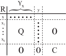
Figure 63: Relation $R$ decomposed as for the proof of Corollary 82.

Since $R$ is connected, $C$ cannot exist and the corollary follows, somewhat as in the proof of Theorem 74 as shown in Figure 62 on page 62.

In order to establish the claim, suppose that $Y_{x}=\{y_{1},\ldots,y_{k}\}$. Suppose further that for each $i=1,\ldots,k$, individual $x_{i}$ has all the attributes of $Y_{x}$ except for $y_{i}$. Now let $y$ be $x_{2}$’s attribute outside $Y_{x}$. We can assume without loss of generality that $x_{1}$ does not have this attribute, and then derive a contradiction, as follows:

Let $X_{\rm imply}=X_{y_{3}}\,\cap\,X_{y}$. The intersection is well-defined since $k\geq 3$. Moreover, $x_{2}\in X_{\rm imply}$, since $x_{2}$ has attributes $y_{3}$ and $y$. However, $x_{1}\not\in X_{\rm imply}$, since $x_{1}$ does not have attribute $y$.

Observe that $X_{y_{1}}=\{x,x_{2},x_{3},\ldots,x_{k}\}$  and  $X_{y_{3}}=\{x,x_{1},x_{2},\ldots,x_{k}\}\setminus\{x_{3}\}$.

Thus $\emptyset\neq X_{\rm imply}=X_{y_{3}}\cap X_{y}\subseteq X_{y_{1}}$.  In other words, attributes $y_{3}$ and $y$ imply attribute $y_{1}$, contradicting the assumption that $R$ preserves attribute privacy. ∎

We turn now to the proof of Theorem 76, which we had stated previously on page 76:

Proof.

Part (i) follows from the Subclaim on page C.3 and part (ii) follows from Lemma 64 on page 64.  We therefore focus on proving part (iii), assuming parts (i) and (ii) hold:

The proof is by induction on $n=\lvert X\rvert=\lvert Y\rvert$.

I. The base case $n=2$ means $R$ is isomorphic to a standard two element diagonal relation as on page 64, which preserves association privacy.

II. For the induction step, assume that, for some $n>2$, part (iii) of the theorem holds for all relations with $X$ and $Y$ spaces of size strictly less than $n$ (and bigger than 1). We need to establish part (iii) for all relations with $X$ and $Y$ spaces of size $n$.

As we observed in the proof of Lemma 78, if ${k_{max}}=1$ in Definition 77, then every individual has exactly one attribute and $R$ is isomorphic to a square diagonal relation, hence preserves association privacy. We therefore assume that ${k_{max}}>1$ for the rest of the proof.

Let ${Q_{max}}$ be as in Definition 77 and consider the decomposition of $R$ as in Figure 64.

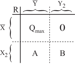
Figure 64: Relation $R$ decomposed into blocks by ${Q_{max}}$.

Here $X_{2}=X\setminus\overline{X}$ and $Y_{2}=Y\setminus\overline{Y}$, with $\overline{X}$ and $\overline{Y}$ as in Definition 77. Then $A$ is the restriction of $R$ to $X_{2}\times\overline{Y}$ and $B$ is the restriction of $R$ to $X_{2}\times Y_{2}$.

Given parts (i) and (ii), Lemma 78 tells us that ${Q_{max}}$ is tight and preserves attribute privacy. By Theorem 65 on page 65, we see that $\lvert\overline{X}\rvert\geq\lvert\overline{Y}\rvert$ and therefore that $\lvert X_{2}\rvert\leq\lvert Y_{2}\rvert$, since $\lvert X\rvert=\lvert Y\rvert$.

Let us look at some cases:

• $\lvert Y_{2}\rvert=\lvert X_{2}\rvert=1$:  Then $B$ is a singleton, so $A=\emptyset$, since $R$ preserves attribute privacy. The induction hypothesis applies to ${Q_{max}}$, telling us that ${Q_{max}}$ preserves association privacy. Since $R$ is the disjoint union of ${Q_{max}}$ and $B$, both nonvoid, we see that $R$ must also preserve association privacy.

• $\lvert Y_{2}\rvert=\lvert X_{2}\rvert>1$:  Arguing as on page C.3, we see that $B$ preserves attribute privacy. Lemmas 64 and 60, on pages 64 and 60, respectively, then imply that $A=\emptyset$. The induction hypothesis applies to each of ${Q_{max}}$ and $B$, since neither is now a singleton (since ${k_{max}}>1$). Again, $R$ is a disjoint union of these two relations, so we see that $R$ preserves association privacy. (One can formalize that argument by using the dual version of Lemma 60 on page 60.)

• $\lvert Y_{2}\rvert>\lvert X_{2}\rvert\geq 1$:  This case cannot occur, since $B$ would preserve attribute privacy but have more attributes than individuals (see again also Theorem 65 on page 65).

• $\lvert X_{2}\rvert=0$:  Then $Y_{2}=\emptyset$ and ${Q_{max}}=R$.

  If $R$ has more than one connected component, then one can apply the induction hypothesis to each component separately. (In order to apply the induction hypothesis, one should first make a small argument that each component is a tight square relation, contains more than one entry, and preserves attribute privacy. This is straightforward.) One concludes that each component preserves association privacy and therefore that $R$ preserves association privacy.

  Otherwise, $R$ is square, tight, connected, and preserves attribute privacy. Furthermore, every row of $R$ has exactly ${k_{max}}$ entries. By assumption, ${k_{max}}>1$ in this part of the proof. So Corollaries 81 and 82 tell us that $R$ is isomorphic to either a cyclic staircase relation or a spherical boundary relation. Thus $R$ preserves association privacy.

∎

Appendix F Poset Chains

Recall Definition 13, on page 13, of the Galois lattice $P^{+}_{R}$ associated with a relation $R$, and Definition 14, on page 14, defining informative attribute release sequences. In this appendix we will explore connections between these two concepts.

F.1 Maximal Chains and Informative Attribute Release Sequences

Let $R$ be a relation on ${X}\mskip-1.8mu\times{Y}$, with both $\hbox{\hskip 1.0pt}{}X$ and $Y\mskip-1.5mu$ nonempty:

Suppose $\{(\sigma_{k},\gamma_{k})<\cdots<(\sigma_{1},\gamma_{1})<(\sigma_{0},\gamma_{0})\}$, with $k\geq 1$, is a maximal chain in $P^{+}_{R}$.

Then,  for $1\leq i\leq k$,  $\sigma_{i}\subsetneq\sigma_{i-1}$ and $\gamma_{i}\supsetneq\gamma_{i-1}$.

Also, $\sigma_{0}=X$ and $\gamma_{k}=Y$, so $\gamma_{0}=\phi_{R}(X)$ and $\sigma_{k}=\psi_{R}(Y)$.

Consequently, $\hbox{\hskip 1.0pt}\gamma_{0}\neq\emptyset\hbox{\hskip 1.0pt}$ if and only if $\mskip 1.0mu{}X\mskip-2.0mu\in\Psi_{R}$, and $\sigma_{k}\neq\emptyset\hbox{\hskip 1.0pt}$ if and only if $\mskip 1.5mu{}Y\mskip-2.0mu\in\Phi_{R}$.

We sometimes speak of a maximal chain at and above $(\sigma,\gamma)$, by which we mean a chain $\{(\sigma,\gamma)<\cdots<(\sigma_{1},\gamma_{1})<(\sigma_{0},\gamma_{0})\}$ in $P^{+}_{R}$ that is maximal among all chains in $P^{+}_{R}$ containing $(\sigma,\gamma)$ as least element. Such a chain is a prefix of a full maximal chain in $P^{+}_{R}$ (“prefix” with respect to our subscript ordering, which starts at the top of a poset and moves downward).

Recall the following lemma, previously stated on page 21 in Section 10.6:

Lemma 21 (Informative Attributes from Maximal Chains).

Let $R$ be a relation on ${X}\mskip-1.8mu\times{Y}$, with both $\hbox{\hskip 1.0pt}{}X\!$ and $\hbox{\hskip 1.0pt}{}Y\!$ nonempty. Suppose $\{(\sigma_{k},\gamma_{k})<\cdots<(\sigma_{1},\gamma_{1})<(\sigma_{0},\gamma_{0})\}$, with $k\geq 1$, is a maximal chain in $P^{+}_{R}$.

Define $y_{1},\ldots,y_{k}$ by selecting some $y_{i}\in\gamma_{i}\setminus\gamma_{i-1}$, for each $i=1,\ldots,k$.

Then $y_{1},\ldots,y_{k}$ is an informative attribute release sequence for $R$.

Moreover, $(\phi_{R}\circ\psi_{R})(\{y_{1},\ldots,y_{i}\})=\gamma_{i}$, for each $i=0,1,\ldots,k$.

Proof.

Establishing the “Moreover” also establishes the “iars” assertion.

The proof is by induction on $i$.

For the base case, $i=0$ and we need to show that $(\phi_{R}\circ\psi_{R})(\emptyset)=\gamma_{0}$.

Calculating, $(\phi_{R}\circ\psi_{R})(\emptyset)=\phi_{R}(X)=\gamma_{0}$, by our earlier comments about maximal chains.

For the induction step, we assume that, for some $1\leq i\leq k$, the assertion holds for indices smaller than $i$ and we need to show the assertion holds for $i$. First, observe:

$$\psi_{R}(\{y_{1},\ldots,y_{i}\})\;=\;\psi_{R}(\{y_{1},\ldots,y_{i-1}\})\;\cap\;X_{y_{\scriptstyle i}}\;=\;\psi_{R}(\gamma_{i-1})\;\cap\;X_{y_{\scriptstyle i}}\;=\;\psi_{R}(\gamma_{i-1}\cup\{y_{i}\}).$$

(The middle equality follows from the induction hypothesis and a dual version of Corollary 46 from page 46, specifically because $(\phi_{R}\circ\psi_{R})(\{y_{1},\ldots,y_{i-1}\})=\gamma_{i-1}$ and $\psi_{R}\circ\phi_{R}\circ\psi_{R}=\psi_{R}$.)

Since $\gamma_{i-1}\subsetneq\gamma_{i-1}\cup\{y_{i}\}\subseteq\gamma_{i}$,

$$\gamma_{i-1}\;=\;(\phi_{R}\circ\psi_{R})(\gamma_{i-1})\;\subsetneq\;(\phi_{R}\circ\psi_{R})(\gamma_{i-1}\cup\{y_{i}\})\;\subseteq\;(\phi_{R}\circ\psi_{R})(\gamma_{i})\;=\;\gamma_{i}.$$

By maximality of the original chain and the nature of elements in $P^{+}_{R}$, we see that $(\phi_{R}\circ\psi_{R})(\gamma_{i-1}\cup\{y_{i}\})=\gamma_{i}$, so $(\phi_{R}\circ\psi_{R})(\{y_{1},\ldots,y_{i}\})=(\phi_{R}\circ\psi_{R})(\gamma_{i-1}\cup\{y_{i}\})=\gamma_{i}$. ∎

Here is a partial converse (also previously stated in Section 10.6):

Lemma 22 (Chains from Informative Attributes).

Let $R$ be a relation on ${X}\mskip-1.8mu\times{Y}$, with both $\hbox{\hskip 1.0pt}{}X$ and $\hbox{\hskip 1.0pt}{}Y\!$ nonempty. Suppose $y_{1},\ldots,y_{k}$ is an informative attribute release sequence for $R$, with $k\geq 1$.

Let $\gamma_{i}=(\phi_{R}\circ\psi_{R})(\{y_{1},\ldots,y_{i}\})$ and $\sigma_{i}=\psi_{R}(\gamma_{i})$, for $i=1,\ldots,k$.

Let $\gamma_{0}=\phi_{R}(X)$.  Then $\{(\sigma_{k},\gamma_{k})<\cdots<(\sigma_{1},\gamma_{1})<(X,\gamma_{0})\}$ is a chain in $P^{+}_{R}$.

Comment: The resulting chain need not be maximal.

Proof.

Observe that each $(\sigma_{i},\gamma_{i})\in P^{+}_{R}$ by construction, so we need to establish the total ordering. Letting $\sigma_{0}=X$, we need to show that $\sigma_{i}\subsetneq\sigma_{i-1}$, for each $i=1,\ldots,k$.

Since $\{y_{1},\ldots,y_{i}\}\supseteq\{y_{1},\ldots,y_{i-1}\}$, we see that $\sigma_{i}\subseteq\sigma_{i-1}$. If $\sigma_{i}=\sigma_{i-1}$, then also $\gamma_{i}=\gamma_{i-1}$, contradicting the fact that $y_{i}\in\gamma_{i}\setminus\gamma_{i-1}$ (which is true by the nature of informative attribute release sequences). ∎

As a corollary to Lemmas 21 and 22, one sees that every informative attribute release sequence (iars) for $R$ is a subsequence of an iars derived from a maximal chain in $P^{+}_{R}$. (Technically, one needs to show that any nonempty subsequence of an iars is itself an iars. And one needs to show that extending any chain obtained via Lemma 22 to a maximal chain retains the original iars as a subsequence of one subsequently obtainable via Lemma 21. All that is straightforward.)

F.2 Chains and Links

We are interested in understanding how chains and informative attribute release sequences behave as one passes to links. (Small caution: whereas we were looking at chains in $P^{+}_{R}$ before, we focus here on $P_{R}$ (and $P_{Q}$).)

Lemma 83 (Chains in Links).

Let $R$ be a relation on ${X}\mskip-1.8mu\times{Y}$, with both $X\!$ and $\hbox{\hskip 1.0pt}{}Y\!$ nonempty, and suppose $(\sigma,\gamma)\in P_{R}$. Let $Q$ be the relation modeling $\mathop{\rm Lk}(\Psi_{R},\sigma)$. Then

$$P_{Q}\;=\;{\left\{(\sigma^{\prime}\setminus\sigma,\,\gamma^{\prime})\;\left|\;(\sigma,\gamma)<(\sigma^{\prime},\gamma^{\prime})\in P_{R}\right.\right\}}.$$

Comments:

• $Q$ is the restriction of $R$ to $\overline{X}\times\gamma$, with $\overline{X}=\bigcup_{y\in\gamma}X_{y}\setminus\sigma$, as per Definition 8 on page 8.

• $P_{Q}$ could be empty. This occurs precisely when $(\sigma,\gamma)$ is a maximal element of $P_{R}$, which occurs precisely when $\mathop{\rm Lk}(\Psi_{R},\sigma)=\{\emptyset\}$, which occurs precisely when $\overline{X}=\emptyset$.

• If $\sigma=X$, then $\mathop{\rm Lk}(\Psi_{R},\sigma)=\{\emptyset\}$ and so $P_{Q}=\emptyset$, given Definition 8 on page 8. (For future reference, observe that $P_{{Q(\sigma,\gamma)}}$ is undefined when $\sigma=X$ and ${Q(\sigma,\gamma)}$ is given by Definition 19 on page 19. See also page • ‣ A.4 for comments about the doubly-labeled poset.)

• $P_{Q}$ never contains the element $\hat{0}_{Q}$ of $P^{+}_{Q}$. Indeed, $\hat{0}_{Q}=(\emptyset,\gamma)$, corresponding to $(\sigma,\gamma)$ in $P_{R}$. That value is consistent with the idea of Lemma 12 on page 12 that one has “localized to $\sigma$ upon observing $\gamma$”. (See also Definition 16 on page 16.)

• $P_{Q}$ could contain the element $\hat{1}_{Q}=(\overline{X},\chi)$ of $P^{+}_{Q}$, for some $\chi\subsetneq\gamma$. That happens precisely when $\overline{X}\neq\emptyset$ and all individuals in $\overline{X}$ share an attribute of $\gamma$, in which case $\chi\neq\emptyset$.

Proof.

The proof relies on dual versions of the formulas appearing in the top half of page • ‣ C.1.

I. Suppose $(\kappa,\eta)\in P_{Q}$. So $\kappa\neq\emptyset$ and $\eta\neq\emptyset$. Also, $\Psi_{Q}=\mathop{\rm Lk}(\Psi_{R},\sigma)$, so $\kappa\cap\sigma=\emptyset$ and $\kappa\cup\sigma\in\Psi_{R}$. Let $\sigma^{\prime}=\kappa\cup\sigma$. So $\sigma\subsetneq\sigma^{\prime}$. We can take $\gamma^{\prime}$ to be $\eta$ since $\eta=\phi_{Q}(\kappa)=\phi_{R}(\sigma^{\prime})$. Note that $\psi_{R}(\gamma^{\prime})=\psi_{Q}(\eta)\cup\sigma=\kappa\cup\sigma=\sigma^{\prime}$. We have shown that $(\sigma^{\prime},\gamma^{\prime})\in P_{R}$ and $(\sigma,\gamma)<(\sigma^{\prime},\gamma^{\prime})$.

II. Suppose $(\sigma^{\prime},\gamma^{\prime})\in P_{R}$ and $(\sigma,\gamma)<(\sigma^{\prime},\gamma^{\prime})$. So $\sigma\subsetneq\sigma^{\prime}$ and $\gamma\supsetneq\gamma^{\prime}$. Let $\kappa=\sigma^{\prime}\setminus\sigma$. Note that $\kappa\neq\emptyset$ and $\gamma^{\prime}\neq\emptyset$. Moreover, $\kappa\in\mathop{\rm Lk}(\Psi_{R},\sigma)$, so $\overline{X}\neq\emptyset$.

Verifying correspondence: $\phi_{Q}(\kappa)=\phi_{R}(\sigma^{\prime})=\gamma^{\prime}$ and $\psi_{Q}(\gamma^{\prime})=\psi_{R}(\gamma^{\prime})\setminus\sigma=\sigma^{\prime}\setminus\sigma=\kappa$.

We have shown that $(\sigma^{\prime}\setminus\sigma,\,\gamma^{\prime})\in P_{Q}$. ∎

Corollary 84 (Order Preservation).

Let $R$ and $Q$ be as in Lemma 83, with $(\sigma,\gamma)\in P_{R}$.

Then $(\sigma,\gamma)<(\sigma_{1},\gamma_{1})<(\sigma_{2},\gamma_{2})$ in $P_{R}$ if and only if  $(\sigma_{1}\setminus\sigma,\,\gamma_{1})<(\sigma_{2}\setminus\sigma,\,\gamma_{2})$ in $P_{Q}$.

Proof.

By Lemma 83 and because:
                      (a) $\sigma\subsetneq\sigma_{1}\subsetneq\sigma_{2}$  implies  $\emptyset\,\neq\,\sigma_{1}\setminus\sigma\,\subsetneq\,\sigma_{2}\setminus\sigma$ ;
                      (b) $\emptyset\neq\kappa_{1}\subsetneq\kappa_{2}$  and  $\kappa_{2}\cap\sigma=\emptyset$   implies  $\sigma\,\subsetneq\,(\kappa_{1}\cup\sigma)\,\subsetneq\,(\kappa_{2}\cup\sigma)$. ∎

Corollary 85 (Maximal Chain Preservation).

Let $R$ and $Q$ be as in Lemma 83, with $(\sigma,\gamma)\in P_{R}$. Then $\{(\sigma,\gamma)<(\sigma_{k},\gamma_{k})<\cdots<(\sigma_{1},\gamma_{1})\}$ is a maximal chain at and above $(\sigma,\gamma)$ in $P_{R}$ if and only if $\{(\sigma_{k}\setminus\sigma,\,\gamma_{k})<\cdots<(\sigma_{1}\setminus\sigma,\,\gamma_{1})\}$ is a maximal chain in $P_{Q}$.

Proof.

By Lemma 83 and Corollary 84, we know that $\{(\sigma,\gamma)<(\sigma_{k},\gamma_{k})<\cdots<(\sigma_{1},\gamma_{1})\}$ is a chain extending upward from $(\sigma,\gamma)$ in $P_{R}$ if and only if $\{(\sigma_{k}\setminus\sigma,\,\gamma_{k})<\cdots<(\sigma_{1}\setminus\sigma,\,\gamma_{1})\}$ is a chain in $P_{Q}$.

Maximality follows for the same reason: Refine or extend a chain in one poset and one can refine or extend the corresponding chain in the other poset as well. ∎

Comment about “length”:

Recall that the length of a chain in a poset is one less than the number of elements in the chain. We also speak of the length of an informative attribute release sequence $y_{1},\ldots,y_{k}$, which is $k$, the actual number of attributes in the sequence.

In the context of Lemmas 21 and 22, there is a happy alignment of definitions: The length $k$ of a longest iars for $R$ is the length $\ell(P^{+}_{R})$.

In thinking about poset lengths, bear in mind that $\ell(P^{+}_{R})$ may be any of $\ell(P_{R})$, $\ell(P_{R})+1$, or $\ell(P_{R})+2$, depending on whether the top and/or bottom elements of $P^{+}_{R}$ already lie in $P_{R}$.

Corollary 86 (Longest Localization Sequences).

Let $R$ be a relation on ${X}\mskip-1.8mu\times{Y}$, with both $X$ and $\hbox{\hskip 1.0pt}{}Y\!$ nonempty, and suppose $(\sigma,\gamma)\in P_{R}$. Let $Q$ be the relation modeling $\mathop{\rm Lk}(\Psi_{R},\sigma)$.

If $X\not\in\Psi_{R}$, then the length of a longest informative attribute release sequence for localizing to $\sigma$ in $R$ is $\ell(P_{Q})+2$.  If $X\in\Psi_{R}$ and $\sigma\neq X$, then that length is $\ell(P_{Q})+1$.

(Note: If $\,\sigma=X\in\Psi_{R}$, then the length is 0; one can localize to $X\!$ in $R$ without observation.)

Comment: If $P_{Q}$ does not contain the top element $\hat{1}_{Q}$ of $P^{+}_{Q}$, then $\ell(P_{Q})+2=\ell(P^{+}_{Q})$, since $P_{Q}$ never contains the bottom element $\hat{0}_{Q}$. This occurs precisely when no attribute is shared by all the individuals in the link.  Also, if $\sigma\subsetneq X\in\Psi_{R}$, then $\ell(P_{Q})+1=\ell(P^{+}_{Q})$.

Proof.

Let us address one special case first, namely when $\mathop{\rm Lk}(\Psi_{R},\sigma)$ is an empty complex. We only care about the situation in which $\sigma$ is not all of $X$, which implies $X\not\in\Psi_{R}$.  Observe that $P_{Q}$ is empty, so $\ell(P_{Q})=-1$ and $\ell(P_{Q})+2=1$. Observe further that any $y\in\gamma$ identifies $\sigma$, as otherwise $\overline{X}$ in the definition of $Q$ would not be empty.  So the Corollary holds in this case.

Suppose $\mathop{\rm Lk}(\Psi_{R},\sigma)$ is not an empty complex and that $X\not\in\Psi_{R}$. Lemmas 21 and 22 imply that a longest informative attribute release sequence for localizing to $\mskip 1.0mu\sigma\mskip-1.0mu$ comes from a longest maximal chain in $P^{+}_{R}$ at and above $(\sigma,\gamma)$. Thus, by Corollary 85, this sequence arises from a maximal chain in $P_{Q}$, augmented by considering also $\hat{0}_{Q}$ and $\hat{1}_{R}$. The length of the chain in $P_{Q}$ is two shorter than that in $P^{+}_{R}$. Why? Because $(\sigma,\gamma)\in P^{+}_{R}$     becomes $\hat{0}_{Q}\in P^{+}_{Q}$, which is not present in $P_{Q}$, and because the top element $\hat{1}_{R}=(X,\emptyset)\in P^{+}_{R}$ disappears altogether ($\hat{1}_{Q}$ may or may not be in $P_{Q}$).   So $\ell(P_{Q})+2$ gives the correct length of the iars for $R$.    

Suppose $\mathop{\rm Lk}(\Psi_{R},\sigma)$ is not an empty complex but that $\sigma\subsetneq X\in\Psi_{R}$. The argument proceeds as before except that now the top element of $P^{+}_{R}$ looks like $\hat{1}_{R}=(X,\gamma_{0})$, with $\gamma_{0}\neq\emptyset$. It appears in $P_{R}$. Consequently, $\hat{1}_{Q}=(X\setminus\sigma,\,\gamma_{0})$ and so $\hat{1}_{Q}$ also appears in $P_{Q}$. So a maximal chain in $P_{Q}$ is now only one shorter than a corresponding maximal chain in $P^{+}_{R}$ at and above $(\sigma,\gamma)$, meaning $\ell(P_{Q})+1$ gives the correct length of a longest iars. ∎

F.3 Isotropy

We turn now to the proof of our isotropy sphere theorem, with the theorem replicated here from earlier in the report. Recall also Definitions 14, 15, 16, and 19 from pages 14–19.

Theorem 20 (Isotropy = Minimal Identification = Sphere).

Let $R$ be a relation and suppose $\emptyset\neq\gamma\in\Phi_{R}$.  Let $\sigma=\psi_{R}(\gamma)$. Then the following four conditions are equivalent:

1. $\gamma$ is isotropic.

2. $\gamma$ is minimally identifying (for $\sigma$).

3. $\Psi_{Q(\sigma,\gamma)}\;\simeq\;\mathbb{S}^{\kern 0.56001pt{k-2}}$, with $k=\lvert\gamma\rvert$.

4. $\Phi_{Q(\sigma,\gamma)}\;=\;\partial(\gamma)$.

Proof.

Observe that $\sigma\in\Psi_{R}$   and $\gamma\subseteq(\phi_{R}\circ\psi_{R})(\gamma)=\phi_{R}(\sigma)$, so constructing ${Q(\sigma,\gamma)}$ is valid. Also, (a)–(d) each imply $\sigma\neq X$. Finally, observe that $\gamma\not\in\Phi_{Q(\sigma,\gamma)}$. For if there were some $x\in\overline{X}$ such that $(x,y)\in{Q(\sigma,\gamma)}\subseteq R$ for every $y\in\gamma$, then $x\in\sigma$, but $\sigma$ is disjoint from $\overline{X}$.

If $\lvert\gamma\rvert=1$, then $\mathbb{S}^{\kern 0.56001pt{k-2}}=\mathbb{S}^{\kern 0.56001pt{-1}}=\{\emptyset\}=\partial(\gamma)$. Write $\gamma=\{y\}$. Then $\gamma$ is isotropic if and only if $y$ constitutes an informative attribute release sequence, if and only if $y\not\in\phi_{R}(X)$. If $y\in\phi_{R}(X)$, then $\sigma=X$, so our conventions say $\Psi_{Q(\sigma,\gamma)}\!=\emptyset\not\simeq\{\emptyset\}$ and $\Phi_{Q(\sigma,\gamma)}=\emptyset\neq\{\emptyset\}$. Moreover, $\psi_{R}(\emptyset)=\sigma$, so $\gamma$ is not minimally identifying. If $y\not\in\phi_{R}(X)$, then $\sigma=X_{y}\subsetneq X$ and $\overline{X}=\emptyset$, so both $\Psi_{Q(\sigma,\gamma)}$ are $\Phi_{Q(\sigma,\gamma)}$ are instances of $\{\emptyset\}$, by our conventions.     Moreover, $X=\psi_{R}(\emptyset)\supsetneq\sigma$.  So we see that (a), (b), (c), (d) are all equivalent when $\lvert\gamma\rvert=1$.     

Henceforth assume that $\lvert\gamma\rvert>1$. It will be convenient to write $\gamma=\{y_{1},\ldots,y_{k}\}$, with $k>1$, and with the attribute indexing chosen arbitrarily.

As we have observed elsewhere, (c) and (d) are equivalent by Dowker duality and the fact that only a boundary complex can produce $\mathbb{S}^{\kern 0.56001pt{k-2}}$ homotopy type when the underlying vertex set has size $k$.

We will first show that (a) implies (d) and (b):

Suppose that $\gamma$ is isotropic.

We wish to show that all proper subsets of $\gamma$ are simplices in $\Phi_{Q(\sigma,\gamma)}$. Without loss of generality, consider $\{y_{1},\ldots,y_{k-1}\}$. If we can show that $\psi_{R}(\{y_{1},\ldots,y_{k-1}\})\setminus\sigma\neq\emptyset$, then that provides an $x\in\overline{X}$ such that $(x,y_{i})\in R$ for $i=1,\ldots,k-1$, thereby establishing that $\{y_{1},\ldots,y_{k-1}\}\in\Phi_{Q(\sigma,\gamma)}$. It also establishes that $\psi_{R}(\{y_{1},\ldots,y_{k-1}\})\supsetneq\sigma$. Since the “missing attribute” $y_{k}$ is arbitrary in $\gamma$, we see that $\Phi_{Q(\sigma,\gamma)}=\partial(\gamma)$ and that $\gamma$ is minimally identifying.

Suppose otherwise: $\psi_{R}(\{y_{1},\ldots,y_{k-1}\})=\sigma=\psi_{R}(\gamma)$, so also $(\phi_{R}\circ\psi_{R})(\{y_{1},\ldots,y_{k-1}\})=(\phi_{R}\circ\psi_{R})(\gamma)\supseteq\gamma$. That says $y_{k}\in(\phi_{R}\circ\psi_{R})(\{y_{1},\ldots,y_{k-1}\})$, violating the assumption that any ordering of $\gamma$ is an informative attribute release sequence.

We will now show that (d) implies (a):

Suppose that $\Phi_{Q(\sigma,\gamma)}=\partial(\gamma)$.

If some ordering of $\gamma$ is not an informative attribute release sequence, then we can rearrange the sequence further to establish that the last attribute is implied by all the others, i.e., that $y_{k}\in(\phi_{R}\circ\psi_{R})(\{y_{1},\ldots,y_{k-1}\})$. Arguing as we did in the proof of Lemma 21 on page F.1, we obtain:

$$\psi_{R}\big{(}\{y_{1},\ldots,y_{k-1}\}\big{)} = (\psi_{R}\circ\phi_{R})\Big{(}\psi_{R}\big{(}\{y_{1},\ldots,y_{k-1}\}\big{)}\Big{)}$$

$$= \psi_{R}\Big{(}(\phi_{R}\circ\psi_{R})\big{(}\{y_{1},\ldots,y_{k-1}\}\big{)}\Big{)}$$

$$= \psi_{R}\Big{(}\{y_{k}\}\cup(\phi_{R}\circ\psi_{R})\big{(}\{y_{1},\ldots,y_{k-1}\}\big{)}\Big{)}$$

$$= X_{y_{\scriptstyle k}}\;\cap\;\psi_{R}\Big{(}(\phi_{R}\circ\psi_{R})\big{(}\{y_{1},\ldots,y_{k-1}\}\big{)}\Big{)}$$

$$= X_{y_{\scriptstyle k}}\;\cap\;\psi_{R}\big{(}\{y_{1},\ldots,y_{k-1}\}\big{)}$$

$$= \psi_{R}\big{(}\{y_{1},\ldots,y_{k}\}\big{)}$$

$$= \psi_{R}(\gamma)$$

$$= \sigma.$$

On the other hand, since $\{y_{1},\ldots,y_{k-1}\}\in\Phi_{Q(\sigma,\gamma)}$, there is a witness $x\in\overline{X}$, meaning $x\in\psi_{R}(\{y_{1},\ldots,y_{k-1}\})$, which contradicts $\overline{X}\cap\sigma=\emptyset$.

Finally, we will show that (b) implies (d):

Suppose that $\gamma$ is minimally identifying.

Observe that $\psi_{R}(\{y_{1},\ldots,y_{k-1}\})\supsetneq\sigma$. As above, this establishes $\{y_{1},\ldots,y_{k-1}\}\in\Phi_{Q(\sigma,\gamma)}$, from which we conclude that $\Phi_{Q(\sigma,\gamma)}=\partial(\gamma)$, since the missing attribute $y_{k}$ was arbitrary. ∎

Appendix G Many Long Chains

This appendix provides a proof of Theorem 26 from page 26.

First, we need some tools:

Recall what it means for a poset to be almost a join-based lattice from Definition 25 on page 25.

Definition 87 (Join Completion).

Suppose $P$ is almost a join-based lattice. Let $S$ be a subset of $P$. The bounded join-completion of $S$ in $P$ is the set $S^{\vee}$ defined by:

$$S^{\vee}={\left\{p\in P\;\left|\;\hbox{$p\leq s$, some $s\in S$, and $p=s_{1}\vee\cdots\vee s_{m}$, with each $s_{i}\in S$, and $m\geq 1$}\right.\right\}}.$$

Here and in the rest of this appendix, “ $\leq$” and “$<$” refer to the partial order on $P$, while “$\,\vee$” denotes the resulting join operation on $P\cup\{\hat{1}\}$.  $S$ and $S^{\vee}$ inherit this partial order.

We also define $S_{\max}$ to consist of all the maximal elements of $S$ relative to the partial order inherited from $P$.

The following facts will be useful. Assume $S\subseteq P$, with $P$ almost a join-based lattice. Then:

1. $S^{\vee}$ is almost a join-based lattice. The join operation for elements $p,q\in S^{\vee}$ is given by:

   $$p\,\vee_{S^{\vee}}\,q\;=\;\left\{\,\begin{aligned} &p\vee q,&&\hbox{if $\;p\vee q\;\leq\;s$, for some $s\in{S}$;}\\[4.0pt] &\hat{1},&&\hbox{otherwise.}\\ \end{aligned}\right.$$

2. $S\subseteq S^{\vee}$ and $S_{\max}=(S^{\vee})_{\max}$.

3. $(S^{\vee})^{\vee}=S^{\vee}$.

4. If $T\subseteq S$, then $T^{\vee}\subseteq S^{\vee}$.

5. If $T\subseteq S^{\vee}$ such that $S_{\max}\setminus{T}\neq\emptyset$, then $T^{\vee}\subsetneq S^{\vee}$.

6. Let $\emptyset\neq T\subseteq S$. Then the poset

   $$S_{T}={\left\{p\in S^{\vee}\;\left|\;p\leq t,\,\,\hbox{for all $t\in T$}\right.\right\}}$$

   is almost a join-based lattice. The join operation for elements $p,q\in S_{T}$ is given by:

   $$p\,\vee_{S_{T}}\,q\;=\;\left\{\,\begin{aligned} &p\vee q,&&\hbox{if $\;p\vee q\;\leq\;t$,\, for \!{\em all}\, $t\in T$;}\\[4.0pt] &\hat{1},&&\hbox{otherwise.}\\ \end{aligned}\right.$$

7. Fact 6 holds as well for the poset $S^{\prime}_{T}={\left\{\,p\in S^{\vee}\;\left|\;p<t,\,\,\hbox{for all $t\in T$}\right.\right\}}$,
   now using “$<$” in place of “$\leq$” throughout.

Lemma 88 (Contractibility of Closed Semi-Intervals).

Suppose $\emptyset\neq T\subseteq S\subseteq P$, with $P$ almost a join-based lattice. Define the poset $S_{T}$ as in Fact 6 on page G.

If $S_{T}\neq\emptyset$, then $S_{T}$ is contractible.

Proof.

Suppose $p$ and $q$ are arbitrary elements of $S_{T}$. Every element of $T$ is an upper bound for both $p$ and $q$. Since $T$ is not empty, this means $p\vee q$ exists in $P$ and $p\vee q\leq t$ for all $t\in T$. Since $t\in S$, we have that $p\vee q\in S^{\vee}$ and thus $p\vee q\in S_{T}$ as well. Consequently, the lattice $S_{T}\cup\{\hat{0},\hat{1}\}$ is noncomplemented, implying that $S_{T}$ is contractible, by a fact on page • ‣ A.3. ∎

Intuitively:  $\Delta(S_{T})$ is a cone with apex $\bigwedge{T}$, the meet in $S^{\vee}$ of all the upper bounds $T$.

Caution:  The lemma need not  hold for $S^{\prime}_{T}$ as defined in Fact 7 on page G.

We now specialize a topological tool to our current setting. We refer to the lemma as “cycle tightening” because we will apply the lemma with $p\in S_{\max}$ and with $z$ a reduced homology generator for $\Delta(P)$. The lemma will allow us to move that generator downward in $P$.

Lemma 89 (Cycle Tightening).

Let $P$ be almost a join-based lattice. Suppose $z$ is a nontrivial reduced $k$-cycle for $\Delta(P)$, i.e., $0\neq z\in C_{k}(\Delta(P);\mathbb{Z})$ and $\widetilde{\partial}{z}=0$, for some $k\geq 0$.

Define $S=\lVert z\rVert\,$ and $\,K={\left\{\tau\in\Delta(P)\;\left|\;\tau\subseteq S^{\vee}\right.\right\}}$.

Let $p\in S$.

If $\widetilde{H}_{k-1}(\mathop{\rm Lk}(K,p);\mathbb{Z})=0$, then there exists $\eta\in C_{k+1}(\mathop{\rm\overline{St}}(K,p);\mathbb{Z})$ such that $p\notin\lVert z+\widetilde{\partial}\eta\rVert$, now viewing $\eta\in C_{k+1}(\Delta(P);\mathbb{Z})$.

Proof.

Let $W=\mathop{\rm\overline{St}}(K,p)$ and $A=\mathop{\rm Lk}(K,p)$. Note that $A$ is not an empty complex (that observation follows from the reduced homology assumption when $k=0$ and the fact that $p$ is part of a simplex containing at least one other element when $k>0$).

The long exact sequence for a pair [16, 14] therefore gives us the following exact sequence:

$$0=\widetilde{H}_{k}(W;\mathbb{Z})\longrightarrow\widetilde{H}_{k}(W,A;\,\mathbb{Z})\longrightarrow\widetilde{H}_{k-1}(A;\mathbb{Z})=0.$$

The left $0$ comes from $W$ being a cone and the right $0$ comes from the lemma’s hypotheses. Consequently, $\widetilde{H}_{k}(W,A;\,\mathbb{Z})=0$.

Suppose $z=\sum_{i}n_{i}\tau_{i}$, for some collection $\{\tau_{i}\}$ of (oriented) $k$-simplices such that $n_{i}\neq 0$ for each $i$. Let $z_{S}$ consist of the part of $z$ that lies within $W$, so:

$$\hskip 144.54ptz_{S}=\sum_{\tau_{\scriptstyle i}\in{W}}n_{i}\tau_{i}\qquad\qquad\hbox{(with each $n_{i}$ and $\tau_{i}$ as in $z$)}.$$

Since $z$ is a reduced $k$-cycle with support in $\mathop{\rm verts}(K)$, $z_{S}$ is a reduced relative $k$-cycle for the pair $(W,A)$.  Since $\widetilde{H}_{k}(W,A;\,\mathbb{Z})=0$, $z_{S}$ must be a reduced relative boundary, so there exists $\kappa\in C_{k+1}(W;\mathbb{Z})$ such that $z_{S}=\widetilde{\partial}\kappa+\gamma$, with $\gamma\in C_{k}(A;\mathbb{Z})$.

Now let $\eta=-\kappa$ and view $\eta\in C_{k+1}(\Delta(P);\mathbb{Z})$.

Observe that $\lVert z_{S}+\widetilde{\partial}\eta\rVert\subseteq\mathop{\rm verts}(A)\subseteq\mathop{\rm verts}(\mathop{\rm dl}(K,p))$. Consequently, $p\not\in\lVert z+\widetilde{\partial}\eta\rVert$. ∎

Lemma 90 (Maximal Element Cardinality).

Let $P$ be almost a join-based lattice. Suppose $P$ has reduced integral homology in dimension $k\geq 0$, that is, $\widetilde{H}_{k}(\Delta(P);\mathbb{Z})\neq 0$.

Let $S=\lVert z\rVert$, with $z\in C_{k}(\Delta(P);\mathbb{Z})$ a reduced homology generator for $\widetilde{H}_{k}(\Delta(P);\mathbb{Z})$.

Then $\lvert S_{\max}\rvert\geq k+2$.

Proof.

Since $S\subseteq S^{\vee}$, we can view $z\in C_{k}(\Delta(S^{\vee});\mathbb{Z})$. If there were to exist $\eta\in C_{k+1}(\Delta(S^{\vee});\mathbb{Z})$ such that $\widetilde{\partial}\eta=z$, then $z$ would also be a reduced boundary in $\Delta(P)$. So, $\widetilde{H}_{k}(\Delta(S^{\vee});\mathbb{Z})\neq 0$ and $z$ is a reduced homology generator for $\Delta(S^{\vee})$.

Recall the notation $S_{T}$ in Fact 6 on page 6.  Observe that

$$\bigcup_{\phantom{000}t\in{{\hbox{\footnotesize$S$}}_{\scriptstyle\max}}}\Delta(S_{\{t\}})\;=\;\Delta(S^{\vee}).$$

To see this, first observe that the empty simplex $\emptyset$ appears in both these sets. Then:

• Suppose $\emptyset\neq\sigma\in\Delta(S_{\{t\}})$ for some $t\in S_{\max}$. Being a chain in $S_{\{t\}}$, we can write $\sigma$ as $\{p_{0}<p_{1}<\cdots<p_{\ell}\}$, for some $\ell\geq 0$, with each $p_{i}\in S^{\vee}$ (and $\,p_{\ell}\leq t\in S_{\max}\subseteq S\subseteq S^{\vee}$).

  Consequently, $\sigma\in\Delta(S^{\vee})$ as well.

• Suppose $\emptyset\neq\sigma\in\Delta(S^{\vee})$. Then $\sigma=\{p_{0}<p_{1}<\cdots<p_{\ell}\}$, for some $\ell\geq 0$, with each $p_{i}\in S^{\vee}$. By definition of $S^{\vee}$ and $S_{\max}$, $p_{\ell}\leq s\leq t$, for some $s\in S$ and $t\in S_{\max}$.

  Consequently, $\sigma\in\Delta(S_{\{t\}})$ as well, for that $t$.

Similarly, one sees that, for any $\emptyset\neq T\subseteq S$,

$$\bigcap_{t\in{T}}\Delta(S_{\{t\}})\;=\;\Delta(S_{T}).$$

The complex on the right is either an empty complex or it is contractible, by Lemma 88.

A variation of the Nerve Lemma now implies that $\Delta(S^{\vee})$ and the nerve of the simplicial complexes $\big{\{}\Delta(S_{\{t\}})\big{\}}_{t\in{\hbox{\footnotesize$S$}}_{\scriptstyle\max}}$ have the same homotopy type (see Theorem 10.6(i) in [1]).

Since $\Delta(S^{\vee})$ has reduced homology in dimension $k$, so does the nerve of $\big{\{}\Delta(S_{\{t\}})\big{\}}_{t\in{\hbox{\footnotesize$S$}}_{\scriptstyle\max}}$.

The nerve of $\big{\{}\Delta(S_{\{t\}})\big{\}}_{t\in{\hbox{\footnotesize$S$}}_{\scriptstyle\max}}$ is isomorphic to a simplicial complex with underlying vertex set $S_{\max}$. In order for a simplicial complex to have reduced homology in dimension $k$, with $k\geq 0$, the complex must have at least $k+2$ vertices. Thus $\lvert S_{\max}\rvert\geq k+2$. ∎

We now turn to the proof of the main theorem, the statement of which is replicated here:

Theorem 26 (Many Maximal Chains).

Let $P$ be almost a join-based lattice. Suppose $P$ has reduced integral homology in dimension $k\geq 0$, that is, $\widetilde{H}_{k}(\Delta(P);\mathbb{Z})\neq 0$.

Then there are at least $(k+2)!$ maximal chains in $P$ of length at least $k$.

Proof.

The proof is by induction on $k$.

I. For the base case, $k=0$, observe that $\Delta(P)$ must have at least two vertices that are incomparable in $P$, as otherwise $\Delta(P)$ would be either empty or contractible. Each vertex sits inside a maximal chain of $P$. The chains are different since the vertices are incomparable.

II. For the induction step, assume that, for some $k\geq 1$, the theorem holds for all relevant $P$ with reduced homology in dimension $k-1$. We need to establish the theorem for all relevant $P$ with reduced homology in dimension $k$.

Let $z=\sum_{i}n_{i}\tau_{i}$ be a reduced homology generator for $\widetilde{H}_{k}(\Delta(P);\mathbb{Z})$, with $n_{i}\neq 0$ for each $i$.

Define $S$ and $K$ by $S=\lVert z\rVert$ and $K={\left\{\tau\in\Delta(P)\;\left|\;\tau\subseteq S^{\vee}\right.\right\}}$. Interpretation:  $S$ is the support of the reduced homology generator $z$ and $K$ is the subcomplex of $\Delta(P)$ formed by restricting to the bounded join-completion of $z$’s support.

We now have an inner induction, which we will describe as an iterative loop:

(Notation: superscript $(j)$ indicates the $j^{\hbox{\footnotesize th}}$ iteration.)

1. Initialize with $z^{(0)}=z$,  $S^{(0)}=S$,  and $K^{(0)}=K$.

2. Suppose $z^{(j)}$,  $S^{(j)}$,  and $K^{(j)}$ have been defined, with $z^{(j)}$ a reduced homology generator for $\widetilde{H}_{k}(\Delta(P);\mathbb{Z})$,   and with $S^{(j)}$ and $K^{(j)}$ similar in meaning to $S$ and $K$, now based on $z^{(j)}$.  In particular, $z^{(j)}$ has support $S^{(j)}$ and all of $K^{(j)}$’s vertices lie in $(S^{(j)})^{\vee}$.

   Pick some $p\in(S^{(j)})_{\max}$ such that $\widetilde{H}_{k-1}(\mathop{\rm Lk}(K^{(j)},p);\mathbb{Z})=0$.

   If no such $p$ exists, then the loop ends.

3. Otherwise, invoke Lemma 89 to find an $\eta\in C_{k+1}(\mathop{\rm\overline{St}}(K^{(j)},p);\mathbb{Z})$ such that $p\notin\lVert z^{(j)}+\widetilde{\partial}\eta\rVert$.

   Let $z^{(j+1)}={z^{(j)}+\widetilde{\partial}\eta}$,  so $z^{(j+1)}$ is again a generator of reduced homology in dimension $k$.   Further, let

   $$\hskip 61.42993ptS^{(j+1)}=\lVert z^{(j+1)}\rVert\hskip 8.67204pt\hbox{and}\hskip 7.22743ptK^{(j+1)}\;=\;{\left\{\tau\in\Delta(P)\;\left|\;\tau\subseteq(S^{(j+1)})^{\vee}\right.\right\}}.$$

Observe that $S^{(j+1)}\;\subseteq\;\lVert z^{(j)}\rVert\cup\lVert\widetilde{\partial}\eta\rVert\;\subseteq\;(S^{(j)})^{\vee}$.

On the other hand, $p\in(S^{(j)})_{\rm max}\setminus{S^{(j+1)}}$. So by Fact 5 on page G, $(S^{(j+1)})^{\vee}\subsetneq(S^{(j)})^{\vee}$.

In other words, the possible vertex set for the simplicial complex shrinks with each iteration, and so the loop must eventually end, $P$ being finite.

Given this iterative algorithm, we can now assume without loss of generality that $\widetilde{H}_{k-1}(\mathop{\rm Lk}(K,p);\mathbb{Z})\neq 0$ for each $p$ that is a maximal element in the support $S$ of the given reduced homology generator $z$.

Observe that $\mathop{\rm Lk}(K,p)={\left\{\tau\in\Delta(P)\;\left|\;\tau\subseteq S^{\vee}\;\hbox{and $s<p$ for every $s\in\tau$}\right.\right\}}$, when $p\in S_{\max}$.

Consequently, $\mathop{\rm Lk}(K,p)=\Delta(Q_{p})$, where $Q_{p}$ is the subposet of $P$ given by

$$Q_{p}\;=\;{\left\{s\in S^{\vee}\;\left|\;s<p\right.\right\}}.$$

By Fact 7 on page G, $Q_{p}$ is itself almost a join-based lattice.

$Q_{p}$ has reduced integral homology in dimension $k-1$, so by the induction hypothesis, there are at least $(k+1)!$ maximal chains in $Q_{p}$ of length at least $k-1$. As the description of $Q_{p}$ makes clear, we can extend each of these chains in $P$ by adding $\,p\,$ as a top element, then further refine and/or extend each chain as needed into a maximal chain in $P$. Distinct chains remain distinct after this augmentation since the process only adds elements of $P$ that lie outside $Q_{p}$.

Consequently, we obtain, for each $p\in S_{\max}$, at least $(k+1)!$ distinct maximal chains in $P$ of length at least $k$, each touching $p$. A maximal chain in $P$ cannot contain more than one element of $S_{\max}$, since such elements are necessarily incomparable. Letting $p$ vary over $S_{\max}$ therefore produces at least $\lvert S_{\max}\rvert\cdot(k+1)!$ distinct maximal chains in $P$ of length at least $k$.

By Lemma 90, $\lvert S_{\max}\rvert\geq k+2$. So $P$ contains at least $(k+2)!$ distinct maximal chains of length at least $k$. ∎

Here are two corollaries, previously stated on page 27 in Section 10.8:

Corollary 27 (Holes Reduce Inference).

Let $R$ be a nonvoid relation. Suppose $P_{R}$ has reduced integral homology in dimension $k\geq 0$. Then there are at least $(k+2)!$ maximal chains in $P_{R}$ of length at least $k$.

Proof.

The assertion follows from Theorem 26, since $P_{R}$ is almost a join-based lattice.

(The join operation is exactly that of $P^{+}_{R}$. In particular, the top element $\hat{1}_{R}$ of $P^{+}_{R}$ is not already in $P_{R}$, since $P_{R}$ has homology, so we may adjoin that as the upper bound $\hat{1}$ for $P_{R}$.) ∎

Recall informative attribute release sequences from Section 10.4 and Appendix F.

Corollary 28 (Holes Defer Recognition).

Let $R$ be a nonvoid relation and let $(\sigma,\gamma)\in P_{R}$.

Define $Q=Q(\sigma,\gamma)$ as per Definition 19 and recall Definition 17, from pages 17–19.

Suppose $P_{Q}$ is well-defined and has reduced integral homology in dimension $k\geq 0$.

Then there are at least $(k+2)!$ distinct informative attribute release sequences $y_{1},\ldots,y_{\ell}$ for $R$, each with $\ell\geq k+2$, such that $\psi_{R}(\{y_{1},\ldots,y_{\ell}\})=\sigma$. Consequently, $\mathop{{\rm r}_{\rm slow}}(\sigma)\geq k+2$.

Proof.

By Corollary 27, $P_{Q}$ contains at least $(k+2)!$ maximal chains of length at least $k$.

The rest of the argument is much like that in the proof of Corollary 86 from page 86:

• Each maximal chain in $P_{Q}$ gives rise to a maximal chain in $P^{+}_{R}$ at or above $(\sigma,\gamma)$.

• Distinctness in $P_{Q}$ carries over to $P^{+}_{R}$.

• In moving from $P_{Q}$ to $P^{+}_{R}$ one adds two elements:

  1. One adds $(\sigma,\gamma)$, corresponding to $\hat{0}_{Q}$ in $P^{+}_{Q}$.

  2. $P_{Q}$ has reduced homology, so no attribute is shared by all individuals, either in $Q$ or in $R$.  One thus also adds the top element $\hat{1}_{R}$ of $P^{+}_{R}$.

Summarizing the length argument: Each distinct maximal chain in $P_{Q}$ of length at least $k$ gives rise to a distinct maximal chain at or above $(\sigma,\gamma)$ in $P^{+}_{R}$ of length at least $k+2$, and therefore a distinct informative attribute release sequence for $R$ of length at least $k+2$. By construction of $Q$ and by Lemma 21 on page F.1, each such iars identifies $\sigma$ in $R$. So by Definition 17, $\mathop{{\rm r}_{\rm slow}}(\sigma)\geq k+2$.

(How do we know that distinct maximal chains produce distinct iars? Because if two iars are the same, the chains must be the same, by the “Moreover” of Lemma 21. It is true that one may be able to obtain different iars from the same maximal chain, but our counting is over maximal chains, so provides a lower bound for the number of distinct iars.) ∎

Comment:

Since $P_{Q}$ is well-defined and has reduced homology in nonnegative dimension, $Q$’s Dowker complexes are neither void nor empty. Thus $\sigma\neq{X}$. Along with the assumption $(\sigma,\gamma)\in P_{R}$, that means relation $Q(\sigma,\gamma)$ models the link $\mathop{\rm Lk}(\Psi_{R},\sigma)$.

Appendix H Obfuscating Strategies

Recall the discussion and terminology of Section 13.

The primary goal of this appendix is to provide a proof of Theorem 32 appearing on page 32. In addition, this appendix provides proof of some of the assertions in the bullets on pages 13.2–• ‣ 13.2.

Once again, we first need to develop some tools:

H.1 Source Complex

Subsection 13.1 introduced the strategy complex $\Delta_{G}$ of a graph $G=(V,{\mathfrak{A}})$. Recall that every action $a\in{\mathfrak{A}}$ has a unique source state in $V$. Given a set of actions ${\mathcal{A}}\subseteq{\mathfrak{A}}$, we define the start region of ${\mathcal{A}}$, denoted by $\mathop{\rm src}({\mathcal{A}})$, as

$$\mathop{\rm src}({\mathcal{A}})\;=\;{\left\{v\in V\;\left|\;\hbox{$v$ is the source state of some action $a\in{\mathcal{A}}$}\right.\right\}}.$$

One obtains another simplicial complex from $G$ via $\mathop{\rm src}$, now on underlying vertex set $V$:

$${\overline{\Delta}_{G}}\;\;={\left\{\mathop{\rm src}(\sigma)\;\left|\;\sigma\in\Delta_{G}\right.\right\}}.$$

We refer to this complex as $G$’s source complex.

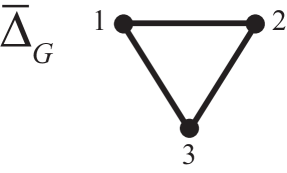
Figure 65: Source complex for the graph of Figure 44 on page 44.

The map $\mathop{\rm src}\!:{\mathfrak{F}}(\Delta_{G})\rightarrow{\mathfrak{F}}({\overline{\Delta}_{G}})$ is a homotopy equivalence, so $\Delta_{G}\simeq{\overline{\Delta}_{G}}$ [6, 7]. Consequently, the source complex of a fully controllable graph $G$ is equal to the boundary complex of the full simplex on the graph’s state space $V$, that is, ${\overline{\Delta}_{G}}={\partial{(V)}}$. For the graph of Figure 44 on page 44, the source complex is the boundary of a triangle, as shown in Figure 65.

$\begin{array}[]{c|ccc}\hbox{\Large$B$}&1&2&3\\[2.0pt] \hline\cr\sigma_{1}&&\bullet&\bullet\\ \sigma_{2}&\bullet&&\bullet\\ \sigma_{3}&\bullet&\bullet&\\ \sigma_{4}&\bullet&\bullet&\\ \end{array}$

$\begin{array}[]{c}\hbox{Goal}\\[2.0pt] \hline\cr 1\\ 2\\ 3\\ 3\\ \end{array}$

Figure 66: Relation $B$ describes the source complex ${\overline{\Delta}_{G}}$ of the graph of Figure 44. Each row describes the start region of a maximal simplex of $\Delta_{G}$, with $\Delta_{G}$ as in Figure 45 on page 45. The rightmost column again shows each maximal strategy’s goal. (See also Figure 46 on page 46.)

In Lemma 30 on page 30 we saw that $\Delta_{G}=\Phi_{A}$ for the action relation $A$ defined there. We now see that ${\overline{\Delta}_{G}}=\Phi_{B}$, with relation $B$ as defined in the next lemma. As example, Figure 66 shows relation $B$ for the graph of Figure 44 from page 44.

Lemma 91.

Let $G=(V,{\mathfrak{A}})$ be a graph as discussed in Section 13.  Let  ${\mathfrak{M}}$ be the set of maximal simplices of $\,\Delta_{G}$.  Define relation $B$ on ${\mathfrak{M}}\times V$ by $B={\left\{(\sigma,v)\;\left|\;v\in\mathop{\rm src}(\sigma)\;\hbox{and}\;\sigma\in{\mathfrak{M}}\right.\right\}}.$

Then $\Phi_{B}={\overline{\Delta}_{G}}$.

(Again, the proof is nearly definitional, so we omit it.)

(The “$B$” stands for “Beginning” — while “$S$” for “source” might be desirable, we have already used $S$ to mean “support” elsewhere.)

How should we interpret the remaining Dowker complexes, $\Psi_{A}$ and $\Psi_{B}$, for relations $A$ and $B$? To answer this question, let us look at the semantics of simplices in these complexes. Suppose $\Delta_{G}$ is not void or empty. A nonempty simplex in $\Psi_{A}$ represents a collection  of maximal simplices of $\Delta_{G}$, namely maximal simplices that have at least one action in common. A nonempty simplex in $\Psi_{B}$ again represents a collection of maximal simplices of $\Delta_{G}$, now with at least one source state in common.  Thus $\Psi_{A}\subseteq\Psi_{B}$.  Moreover, Dowker duality gives:

Lemma 92.

Let $G=(V,{\mathfrak{A}})$ be a graph as discussed in Section 13, with $\mskip 1.0mu{}V\!\neq\emptyset$.

Then the inclusion $\iota:{\mathfrak{F}}(\Psi_{A})\rightarrow{\mathfrak{F}}(\Psi_{B})$ is a homotopy equivalence.

Comment: The assumption $V\!\mskip-1.0mu\neq\emptyset$ means $\Delta_{G}$ and ${\overline{\Delta}_{G}}$ are not void, so relation $B$ is not void. If $\mskip 2.0mu{}V\!\neq\emptyset$ but ${\mathfrak{A}}=\emptyset$, then technically relation $A$ is void, but is is convenient to think of it as an instance of the empty relation instead, with associated empty Dowker complexes.

Proof.

Consider the following diagram:

$$\begin{CD}{\mathfrak{F}}(\Psi_{A})\;\xhookrightarrow{\phantom{01}\iota\phantom{10}}\;{\mathfrak{F}}(\Psi_{B})\phantom{.}\\ @A{\psi_{A}}A{}A@A{\psi_{B}}A{}A\\ {\mathfrak{F}}(\Phi_{A}){\mathfrak{F}}(\Phi_{B})\phantom{.}\\[2.0pt] \hskip 4.0pt\hbox{\Huge\rotatebox{90.0}{$=$}}\hskip 4.0pt\hbox{\Huge\rotatebox{90.0}{$=$}}\phantom{.}\\[-6.0pt] {\mathfrak{F}}(\Delta_{G})\;\xrightarrow{\phantom{0}\mathop{\rm src}\phantom{0}}\;{\mathfrak{F}}({\overline{\Delta}_{G}}).\\ \end{CD}$$

Recall that $\psi_{A}$, $\psi_{B}$, and $\mathop{\rm src}$ are homotopy equivalences.

Let ${\mathfrak{M}}$ denote the maximal simplices of $\Delta_{G}$. Observe the following, for each $\sigma\in{\mathfrak{F}}(\Delta_{G})$:

$(\iota\circ\psi_{A})(\sigma)={\left\{\sigma^{\prime}\in{\mathfrak{M}}\;\left|\;\sigma\subseteq\sigma^{\prime}\right.\right\}}$.

$(\psi_{B}\circ\mathop{\rm src})(\sigma)={\left\{\sigma^{\prime}\in{\mathfrak{M}}\;\left|\;\mathop{\rm src}(\sigma)\subseteq\mathop{\rm src}(\sigma^{\prime})\right.\right\}}$.

If $\sigma\subseteq\sigma^{\prime}$, then $\mathop{\rm src}(\sigma)\subseteq\mathop{\rm src}(\sigma^{\prime})$.

Consequently, $(\iota\circ\psi_{A})(\sigma)\leq(\psi_{B}\circ\mathop{\rm src})(\sigma)$ for every $\sigma\in{\mathfrak{F}}(\Delta_{G})$, where “$\leq$” refers to the partial order on ${\mathfrak{F}}(\Psi_{B})$.

We conclude that the two order-reversing poset maps $\iota\circ\psi_{A}$ and $\psi_{B}\circ\mathop{\rm src}$ are homotopic (see [1], Theorem 10.11) and therefore that $\iota$ is a homotopy equivalence. ∎

Lemma 93.

Let $G=(V,{\mathfrak{A}})$ be a graph as discussed in Section 13, with $\mskip 1.0mu{}V\!\neq\emptyset$.
Then $\,\mathop{\rm src}$ induces a homotopy equivalence of posets $\mskip 2.0muP_{A}\rightarrow P_{B}$ with explicit formula

$$(\tau,\sigma)\mapsto\big{(}(\psi_{B}\circ\mathop{\rm src})(\sigma),(\phi_{B}\circ\psi_{B}\circ\mathop{\rm src})(\sigma)\big{)}.$$

Proof.

Let ${\rm cl}_{A}$ denote the image of the closure operator $\phi_{A}\circ\psi_{A}:{\mathfrak{F}}(\Phi_{A})\rightarrow{\mathfrak{F}}(\Phi_{A})$ and let ${\rm cl}_{B}$ denote the image of the closure operator $\phi_{B}\circ\psi_{B}:{\mathfrak{F}}(\Phi_{B})\rightarrow{\mathfrak{F}}(\Phi_{B})$. We then have the following diagram of homotopy equivalences:

$$P_{A}\xrightarrow{\phantom{01}\pi_{2}\phantom{10}}{\rm cl}_{A}\xhookrightarrow{\phantom{01}\iota\phantom{10}}{\mathfrak{F}}(\Phi_{A})={\mathfrak{F}}(\Delta_{G})\xrightarrow{\phantom{0}\mathop{\rm src}\phantom{0}}{\mathfrak{F}}({\overline{\Delta}_{G}})={\mathfrak{F}}(\Phi_{B})\xrightarrow{\phi_{B}\,\circ\,\psi_{B}}{\rm cl}_{B}\xhookrightarrow{\phantom{01}\iota\phantom{10}}P_{B}.$$

(Here $\pi_{2}$ is projection onto the second coordinate, i.e., $\pi_{2}(\tau,\sigma)=\sigma$, and each of the occurrences of $\iota$ is an inclusion.)

The composition of all these maps is an order-preserving poset map with the specified formula. The overall map is a homotopy equivalence because each of its constituent maps is a homotopy equivalence. ∎

Corollary 94.

If $G$ is fully controllable in Lemma 93, then the formula for the poset map becomes $(\tau,\sigma)\mapsto\big{(}(\psi_{B}\circ\mathop{\rm src})(\sigma),\,\mathop{\rm src}(\sigma)\big{)}.$

Proof.

Since $G$ is fully controllable, $\Phi_{B}={\overline{\Delta}_{G}}={\partial{(V)}}\simeq\mathbb{S}^{\kern 0.56001pt{n-2}}$, with $n=\lvert V\rvert$. So $\Phi_{B}$ has no free faces, implying that $\phi_{B}\circ\psi_{B}$ is the identity, by Lemma 62 on page 62. ∎

Two Observations:  Suppose that $G$ is a fully controllable graph $(V,{\mathfrak{A}})$, with both $V$ and ${\mathfrak{A}}$ nonempty.  (i) No action can appear in all maximal simplices of $\Delta_{G}$, as that would mean $\Delta_{G}$ would be a cone, so not homotopic to a sphere. Consequently, $\hat{1}_{A}=({\mathfrak{M}},\gamma)$ has $\gamma=\emptyset$ (recall that ${\mathfrak{M}}$ is the collection of all maximal simplices of $\Delta_{G}$).  (ii) Even if all actions of ${\mathfrak{A}}$ appear individually as vertices of $\Delta_{G}$, $\hat{0}_{A}=(\tau,{\mathfrak{A}})$ has $\tau=\emptyset$, since $\mathop{\rm src}({\mathfrak{A}})=V$ and $V\notin{\partial{(V)}}$.

These observations mean that $P_{A}$ does not  contain either the top element $\hat{1}_{A}$ or the bottom element $\hat{0}_{A}$ of $P^{+}_{A}$, when $G$ is fully controllable.

H.2 Delaying Strategy Identification

We now turn to the proof of the main theorem, the statement of which is replicated here:

Theorem 32 (Delaying Strategy Identification).

Let $G=(V,{\mathfrak{A}})$ be a fully controllable graph, with $n=\lvert V\rvert>1$. Let $A$ be the relation constructed as in Lemma 30 on page 30 and let $P_{A}$ be its associated doubly-labeled poset. Then:

For each $v\in V$, there exists a maximal strategy $\sigma_{v}\in\Delta_{G}$ for attaining singleton goal state $v$ such that $P_{A}$ contains at least $(n-1)!$ distinct maximal chains for identifying $\sigma_{v}$, with each chain consisting of at least $n-1$ elements.

Proof.

Let $P_{A}^{\rm op}$ be $P_{A}$ but with the opposite partial order. Then $P_{A}^{\rm op}$ is almost a join-based lattice, with join operation for elements of $P_{A}^{\rm op}$ given by

$$(\tau_{1},\sigma_{1})\,\vee\,(\tau_{2},\sigma_{2})\;=\;\left\{\,\begin{aligned} &\big{(}\tau_{1}\cap\tau_{2},\;(\phi_{A}\circ\psi_{A})(\sigma_{1}\cup\sigma_{2})\big{)},&&\hbox{when $\tau_{1}\cap\tau_{2}\neq\emptyset$;}\\[4.0pt] &\hat{1},&&\hbox{otherwise.}\\ \end{aligned}\right.$$

The maximal elements of $P_{A}^{\rm op}$ are of the form $(\{\sigma\},\sigma)$, with $\sigma$ varying over the maximal simplices of $\Delta_{G}$. Each minimal element of $P_{A}^{\rm op}$ is of the form $\big{(}\psi_{A}(\{{\tt a}\}),(\phi_{A}\circ\psi_{A})(\{{\tt a}\})\big{)}$, with action ${\tt a}$ some vertex of $\Delta_{G}$.  (Aside: not every element of that form is necessarily minimal.)

Since $G$ is fully controllable, $\Delta(P_{A}^{\rm op})\simeq\mathbb{S}^{\kern 0.56001pt{n-2}}$. So $\Delta(P_{A}^{\rm op})$ has reduced homology in dimension $k=n-2\geq 0$.  By the proof of Theorem 26, on page G, there exists a reduced homology generator $z$ for $\Delta(P_{A}^{\rm op})$, with support $S=\lVert z\rVert$, such that $P_{A}^{\rm op}$ contains, for each $p\in S_{\max}$, a collection of maximal chains passing through $p$ with the following property: Even if one merely considers the portions of the chains at and below $p$, the collection contains at least $(n-1)!$ distinct such subchains and each subchain has length at least $n-2$. Each full chain, being maximal, must be a path in $P_{A}^{\rm op}$ between some maximal element $(\{\sigma\},\sigma)$ and some minimal element $\big{(}\psi_{A}(\{{\tt a}\}),(\phi_{A}\circ\psi_{A})(\{{\tt a}\})\big{)}$. Working upward from the bottom in $(P_{A}^{+})^{\rm op}$ (which is equivalent to working downward from the top in $P^{+}_{A}$), each such chain therefore gives rise to an informative action release sequence for identifying $\sigma$, consisting of at least $n-1$ actions. Moreover, there are at least $(n-1)!$ different such sequences for that same strategy $\sigma$; we can hold fixed the portion of any chain at and above $p$ in $P_{A}^{\rm op}$, while varying the portion below $p$ in at least $(n-1)!\mskip 0.5mu$ different ways.

Let $p\in S_{\max}$ and suppose $c$ is some maximal chain of $P_{A}^{\rm op}$ that passes through $p$ and touches maximal element $(\{\sigma\},\,\sigma)$. Pick $q\in{S}$, with $q\leq p$ (here, “$\leq$” is the partial order on $P_{A}^{\rm op}$). Write $q=(\tau_{q},\sigma_{q})$ and $p=(\tau_{p},\sigma_{p})$. Even though $q$ may not be part of chain $c$, we can still conclude that $\sigma_{q}\subseteq\sigma_{p}\subseteq\sigma$. If additionally $\mathop{\rm src}(\sigma_{q})=V\setminus\{v\}$, then $\sigma$ at the top of $c$ must be a maximal strategy for attaining singleton goal state $v$. In order to prove the theorem, it is therefore enough to show that, for any $v\in{V}$, some such $q\in{S}$ (and thus $p\in S_{\max}$) exists.

Recall the source relation $B$ from Lemma 91. Let $P_{B}^{\rm op}$ be $P_{B}$ but with the opposite partial order. Referring back to the notation in the proof of Lemma 93, and using the fact that $G$ is fully controllable, one sees that $\Delta(P_{B}^{\rm op})\cong\Delta({\rm cl}_{B})=\Delta({\mathfrak{F}}(\Phi_{B}))=\mathop{\rm sd}({\partial{(V)}})$, with “$\cong$” meaning “isomorphic” and “$\mathop{\rm sd}$” meaning “first barycentric subdivision”. The isomorphism holds by definition of $P_{B}$. The first equality holds because $\phi_{B}\circ\psi_{B}$ is the identity when $G$ is fully controllable, as we saw in the proof of Corollary 94. The second equality amounts to the definition of first barycentric subdivision, bearing in mind that $\Phi_{B}={\overline{\Delta}_{G}}={\partial{(V)}}$.

The homotopy equivalence of Lemma 93 carries over to this setting as $\theta:\Delta(P_{A}^{\rm op})\rightarrow\mathop{\rm sd}({\partial{(V)}})$.  Corollary 94 (or inspection of the diagram in the proof of Lemma 93) provides an explicit formula.  Specifically, for vertices $(\tau,\sigma)$ of $\hbox{\hskip 1.0pt}\Delta(P_{A}^{\rm op})$, one has $\theta(\tau,\sigma)=\mathop{\rm src}(\sigma)$.

Since $\theta$ is a homotopy equivalence, the induced homomorphism $\theta_{*}$ on reduced homology must map the reduced homology generator $z$ to a reduced homology generator for the triangulated $(n\mskip-1.0mu{}-\mskip-1.0mu{}2)$-sphere $\mathop{\rm sd}({\partial{(V)}})$. Consequently, $\lVert\theta_{*}(z)\rVert$ must consist of all vertices in $\mathop{\rm sd}({\partial{(V)}})$, meaning all nonempty proper subsets of $V$. In particular, for each $v\in{V}$, there is some $q=(\tau_{q},\sigma_{q})\in\lVert z\rVert$ such that $\mathop{\rm src}(\sigma_{q})=\theta(q)=V\setminus\{v\}$, as desired. ∎

H.3 Delaying Goal Recognition

The next lemma establishes the “yes” assertion in the bullet that starts near the top of page • ‣ 13.2.

Definition 95 (Complete Strategy).

Let $G=(V,{\mathfrak{A}})$ be a graph as discussed in Section 13. A complete strategy for attaining state $v$ is a strategy $\sigma$ that has at least one action at every state other than $v$.  In other words, $\sigma\in\Delta_{G}$ and $\,\mathop{\rm src}(\sigma)=V\setminus\{v\}$.

Lemma 96 (Delaying Goal Recognition).

Let $G=(V,{\mathfrak{A}})$ be a fully controllable graph.   Let $n=\lvert V\rvert$.  Suppose $n>1$.  Let $s\in V$ be some desired goal state.

There exists a sequence of actions $a_{1},a_{2},\ldots,a_{n-1}$ in ${\mathfrak{A}}$ satisfying the following conditions:

• $\{a_{1},\ldots,a_{n-1}\}$ is a complete strategy for attaining $s$.

• For each $i=1,\ldots,n-1$, let $\tau_{i}=\{a_{1},\ldots,a_{i}\}$ and $W_{i}=\mathop{\rm src}(\tau_{i})$. Then, for each such $i$ and each $v\in V\setminus{W_{i}}$, there exists a complete strategy $\sigma$ for attaining $v$, such that $\tau_{i}\subseteq\sigma\in\Delta_{G}$.

Comments:

(a) Condition (i) implies that no two of the actions $a_{1},\ldots,a_{n-1}$ have the same source state.

(b) Condition (ii) implies that an observer cannot predict the final goal after seeing only a proper prefix of the sequence $a_{1},a_{2},\ldots,a_{n-1}$.

(c) Condition (ii) further implies that the sequence $a_{1},\ldots,a_{n-1}$ forms an informative attribute release sequence for the relation $A$ defined in Lemma 30 on page 30. Again, the reason is that an observer cannot even predict any specific source state for the remaining actions to be released after seeing only a proper prefix of the sequence $a_{1},a_{2},\ldots,a_{n-1}$.

Proof.

For the proof, we assume that ${\mathfrak{A}}$ contains only deterministic and nondeterministic actions, not stochastic ones. The proof generalizes to graphs that include stochastic actions (possibly in addition to deterministic and nondeterministic actions), by an argument in [7]. The essence of that argument is that the source complex of a graph does not change if one replaces stochastic transitions by deterministic ones.

We sketch the rest of the proof, assuming all actions are deterministic or nondeterministic.

Since $G$ is fully controllable, for each state in $V$ there must be a deterministic transition to that state (from some other state). Backchaining such transitions gives rise to a directed cycle of deterministic actions, since the graph is finite. If that cycle is Hamiltonian, then we may choose $a_{1},\ldots,a_{n-1}$ to be any ordering of those $n$ deterministic actions except that we omit the action whose source state is $s$.

Suppose instead that the directed cycle of deterministic actions covers only a proper subset $W$ of the state space $V$. Form a quotient graph with state space $V^{\prime}=\{\diamond\}\cup V\setminus W$, where $\diamond$ represents all of $W$ collapsed to a point. Inductively, the lemma’s assertions hold for the quotient graph. One then needs to show how to combine the actions determined by the quotient graph with the cycle on $W$ in order to satisfy the lemma’s assertions for the original graph $G$. That argument is straightforward if a bit tedious, so we omit it. ∎

H.4 Hamiltonian Flexibility for Strategy Obfuscation

The next lemma establishes the Hamiltonian “yes” in the bullet that starts near the bottom of page 13.2.

Definition 97 (Hamiltonian Action Cycle).

Let $G=(V,{\mathfrak{A}})$ be a graph as in Section 13, possibly with a mix of deterministic, nondeterministic, and stochastic actions. Let $n=\lvert V\rvert$ and assume $n>1$. A sequence of actions $a_{1},\ldots,a_{n}$ in ${\mathfrak{A}}$ is a Hamiltonian cycle of actions  whenever all three of the following conditions hold:

• No two of the actions $a_{1},\ldots,a_{n}$ have the same source state.

• Each action $a_{i}$ is either deterministic or stochastic.

• The source of action $a_{i+1}$ is a target of action $a_{i}$, for all $i=1,\ldots,n-1$, and the source of $a_{1}$ is a target of $a_{n}$.

Observe:

Any proper subset of a Hamiltonian cycle of actions is a simplex in $\Delta_{G}$.

(That observation requires understanding the definition of $\Delta_{G}$ when stochastic actions are involved: stochastic cycles are fine, so long as they are not recurrent. See [7] for details.)

Lemma 98 (Delaying Identification of a Given Strategy).

Let $G=(V,{\mathfrak{A}})$ be a fully controllable graph.  Assume ${\mathfrak{A}}$ contains a Hamiltonian cycle of actions $a_{1},\ldots,a_{n}$, with $n=\lvert V\rvert>1$.

Let $v\in V$ and suppose $\sigma_{v}$ is a maximal and complete strategy in $\Delta_{G}$ for attaining $v$. Then $\sigma_{v}\!$ contains actions $b_{n-1},\ldots,b_{1}$ that constitute a complete strategy for attaining $v$ and that form an informative attribute release sequence for relation $A$.

(Recall: Relation $A$ was defined in Lemma 30 on page 30; it models the maximal simplices of $\Delta_{G}$ in terms of their constituent actions.)

Proof.

Let $v$ and $\sigma_{v}$ be as specified.

We can assume without loss of generality that $V=\{1,\ldots,n\}$, that the source of $a_{i}$ is $i$ for all $i\in V$, and that $v=n$.

Now let $b_{1},\ldots,b_{n-1}$ be any actions in $\sigma_{v}$ chosen so that the source of $b_{i}$ is $i$, for $i=1,\ldots,n-1$.  (If $b_{i}=a_{i}$ for some or all $i$, that is fine.)

Then $\{b_{1},\ldots,b_{n-1}\}$ is itself a complete strategy for attaining $v$.

We claim that the release order $b_{n-1},\ldots,b_{1}$ constitutes an informative attribute release sequence for relation $A$. In fact, we will prove the stronger assertion:

Claim:   Pick some $i\in\{1,\ldots,n\}$.  Then: For each $s\in\{n\}\cup\{1,\ldots,i-1\}$, there exists a complete strategy $\sigma_{s}\in\Delta_{G}$ for attaining $s$, with $\{b_{i},b_{i+1},\ldots,b_{n-1}\}\subseteq\sigma_{s}$. (Notation: $\{b_{i},b_{i+1},\ldots,b_{n-1}\}=\emptyset$ when $i=n$. Similarly for other sets.)

Consequently, an observer cannot predict a specific source state for the remaining actions to be released after seeing a proper prefix of $b_{n-1},\ldots,b_{1}$, so the action sequence is informative.

The claim certainly holds for $s=n$, using the original $\sigma_{v}$. Now consider an $s\in\{1,\ldots,i-1\}$ and let $\sigma_{s}=\{a_{1},\ldots,a_{s-1}\}\cup\{b_{s+1},\ldots,b_{n-1}\}\cup\{a_{n}\}$. By arguments from [7], $\sigma_{s}\in\Delta_{G}$. Finally, observe that $\mathop{\rm src}(\sigma_{s})=V\setminus\{s\}$ and that $\sigma_{s}$ contains $\{b_{i},b_{i+1},\ldots,b_{n-1}\}$. ∎

Caution: As mentioned on page 13.2, just because $b_{n-1},\ldots,b_{1}$ as produced by Lemma 98 is an informative attribute release sequence for $A$, that does not mean one should always release actions in that fashion. If the release protocol were so rigid, an adversary familiar with the protocol would be able to infer much about the goal. In particular, the target set of $a_{n-1}$ includes the goal state, so if that action is deterministic and if always $b_{n-1}=a_{n-1}$, then the adversary would be able to infer at least the goal from the first action released.

H.5 Example: A Rapidly Inferable Strategy

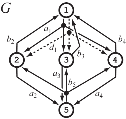
Figure 67: A graph with five states $\{1,2,3,4,5\}$, six deterministic actions $\{a_{2},a_{3},a_{4},b_{2},b_{3},b_{4}\}$, two nondeterministic actions $\{a_{1},b_{5}\}$, and one stochastic action $\{d_{1}\}$.

Figure 67 shows a fully controllable graph on fives states. The graph contains six deterministic actions, two nondeterministic actions, and one stochastic action. (See [6, 7] to learn more about graphs that contain deterministic, nondeterministic, and stochastic actions.) The action relation $A$ for the graph appears in Figure 68.

$\begin{array}[]{c|ccccccccc}A&a_{1}&a_{2}&a_{3}&a_{4}&d_{1}&b_{2}&b_{3}&b_{4}&b_{5}\\[2.0pt] \hline\cr\sigma_{1}&&&&&&\bullet&\bullet&\bullet&\bullet\\[2.0pt] \sigma_{2}&&&&&\bullet&&\bullet&\bullet&\bullet\\[2.0pt] \sigma_{3}&&&&&\bullet&\bullet&&\bullet&\bullet\\[2.0pt] \sigma_{4}&&&&&\bullet&\bullet&\bullet&&\bullet\\[2.0pt] \sigma_{234}&\bullet&&&&\bullet&&&&\bullet\\[2.0pt] \sigma_{5}&\bullet&\bullet&\bullet&\bullet&\bullet&&&&\\[2.0pt] \sigma_{54}&&\bullet&\bullet&\bullet&\bullet&\bullet&\bullet&&\\[2.0pt] \sigma_{53}&&\bullet&\bullet&\bullet&\bullet&\bullet&&\bullet&\\[2.0pt] \sigma_{52}&&\bullet&\bullet&\bullet&\bullet&&\bullet&\bullet&\\[2.0pt] \sigma_{15}&&\bullet&\bullet&\bullet&&\bullet&\bullet&\bullet&\\[2.0pt] \end{array}$

$\begin{array}[]{c}\hbox{Goal}\\[2.0pt] \hline\cr 1\\[2.0pt] 2\\[2.0pt] 3\\[2.0pt] 4\\[2.0pt] \{2,3,4\}\\[2.0pt] 5\\[2.0pt] 5\\[2.0pt] 5\\[2.0pt] 5\\[2.0pt] \{1,5\}\\[2.0pt] \end{array}$

Figure 68: Relation $A$ describes the strategy complex for the graph of Figure 67 in terms of its maximal strategies and their constituent actions. The rightmost column further shows each maximal strategy’s goal.

Strategy $\sigma_{5}$ is a maximal and complete strategy for attaining state $\{5\}$, consisting of actions $\{a_{1},a_{2},a_{3},a_{4},d_{1}\}$. Observe that a longest informative action release sequence for this strategy has length 3. For instance, $d_{1},a_{2},a_{1}$ is such a sequence. Why is there no informative action release sequence longer than 3? Answer: As soon as one releases any one of the three actions $\{a_{2},a_{3},a_{4}\}$, an observer can infer that the strategy cannot contain the action $b_{5}$ and therefore, being maximal, must contain the other two actions in the set $\{a_{2},a_{3},a_{4}\}$ as well.

On page 13.2 we asked whether one can always find an informative action release sequence of length $n-1$ for a maximal complete strategy. (Here $n$ is the number of states in the graph.) We see now that the answer is “no”, not in general. Key to the current counterexample are two characteristics:

1. The graph contains three equivalent actions, namely $\{a_{2},a_{3},a_{4}\}$: The actions have completely identical columns in relation $A$. One could prune the graph to remove redundant such actions while preserving full controllability, but this would not ensure a “yes” answer in general. The reason is that action equivalence is merely one of an infinite family of inferences one can construct with graphs. For instance, we could build a subgraph with an “any-2-actions-imply-4” character and construct a new counterexample.

2. The actions $a_{1}$ and $d_{1}$ both have source state $1$ and target states $\{2,3,4\}$, yet are not equivalent. The difference is that $a_{1}$ is nondeterministic, meaning that potentially an adversary could determine the target state attained any time the action is executed. In contrast, $d_{1}$ is merely stochastic, meaning each target state has some fixed nonzero probability of occurring any time the action is executed, independent over repeated execution instances.

   If we disallowed the stochastic action $d_{1}$, full controllability would necessitate more deterministic actions in the graph, thereby changing both the collection of maximal simplices and consequent inferences. For instance, we might replace $d_{1}$ by three deterministic transitions. Doing so would similarly change the problematic strategy $\sigma_{5}$, providing more actions and increasing the length of an informative action release sequence for identifying $\sigma_{5}$. We then would indeed obtain an informative action release sequence of length 4. Alternatively, if we disallowed the nondeterministic action $a_{1}$, then the problematic strategy $\sigma_{5}$ would simply disappear. We would not even need to add any other actions, as the graph would remain fully controllable. Whether and when such alternatives are realistic is application dependent. We leave for future work exploration of more detailed conditions under which each maximal complete strategy in a graph has an informative action release sequence of length at least $n-1$. Such characterizations might be useful in designing systems that either are or are not obfuscation-friendly. Appendix H.6 initiates this exploration with a discussion of pure graphs.

H.6 Pure Nondeterministic Graphs and Pure Stochastic Graphs

Let $G=(V,{\mathfrak{A}})$ be a graph whose actions may have uncertain outcomes. We say that $G$ is pure nondeterministic if each action in ${\mathfrak{A}}$ is nondeterministic (for the purposes of this definition, we regard a deterministic action as a special instance of a nondeterministic action). We say that $G$ is pure stochastic if each action in ${\mathfrak{A}}$ is stochastic (now viewing a deterministic action as a special instance of a stochastic action). We may simply say that $G$ is pure  if it is either pure nondeterministic or pure stochastic.

One can prove that every maximal strategy in the strategy complex of a fully controllable pure graph contains an informative action release sequence of length at least $n-1$, with $n=\lvert V\rvert$. This result means that one can release at least $n-1$ actions informatively before an observer can identify the strategy.

We will omit proof details, merely sketch the approach. First, one can show that if the Hamiltonian cycle in Lemma 98 is formed from deterministic actions, then every maximal strategy with a multi-state goal actually contains an informative action release sequence (iars) of length $n$. More specifically, suppose $\sigma$ is such a strategy. The iars for $\sigma$ consists of all the Hamiltonian cycle edges that are in $\sigma$, along with one action in $\sigma$ for each cycle edge that is missing from $\sigma$. At least two such cycle edges are missing, since $\sigma$ has at least two goal states. Consequently, the cycle breaks nicely into at least two intervals. For each missing cycle edge $e$, let $I_{e}$ denote the interval of states between $e$’s target and the next missing edge’s source (based on the circular ordering induced by the Hamiltonian cycle). Include the endpoints (these could be identical, which is fine). One knows that every minimal nonface of $\Delta_{G}$ containing $e$ must include some other action whose source lies in $I_{e}$ and whose targets do not  all lie inside $I_{e}$. One can therefore release one such action from $\sigma$ informatively, in place of $e$.

Next, observe that every fully controllable pure nondeterministic graph contains a hierarchical decomposition of nested directed cycles, whose union covers $V$, such that each cycle is deterministic Hamiltonian in the quotient graph formed when one regards each of that cycle’s subcycles as a singleton state. There are some details to verify, but, given a maximal strategy $\sigma$ in the graph’s strategy complex, this hierarchical decomposition and the previous Hamiltonian result yield an informative action release sequence of length at least $n-1$ for $\sigma$.

The approach is different for pure stochastic graphs. A nice property of minimal nonfaces in $\Delta_{G}$, when $G$ is pure stochastic, is that they form irreducible recurrent Markov chains and thus define fully controllable subgraphs of $G$. Moreover, each nonempty proper subset of a minimal nonface defines an isotropic simplex of actions with respect to $G$’s action relation. When $G$ itself is fully controllable, one can patch such subgraphs together expansively. In particular, given a maximal strategy $\sigma$ in $\Delta_{G}$, one can choose as building blocks fully controllable subgraphs that each consist solely of actions in $\sigma$ plus one action not in $\sigma$. One starts by considering an action that moves off a goal state of $\sigma$. That action cannot be in $\sigma$, so gives rise to a minimal nonface all of whose other actions do lie in $\sigma$. One then expands outward repeatedly. Once no additional expansion is possible, one passes to a quotient graph by identifying all states covered thus far. Inductively, one can then repeat the expansion in the quotient graph. Again, there are some details to verify, but ultimately this process covers the graph’s state space and produces an informative action release sequence of length at least $n-1$ for $\sigma$.

H.7 Strategy Obfuscation Summary

We summarize the key points of this appendix with the following theorem:

Theorem 99 (Obfuscation).

Let $G=(V,{\mathfrak{A}})$ be a fully controllable graph, with $n=\lvert V\rvert>1$.

Let $\mskip 2.0mu\sigma\mskip-1.0mu$ be a maximal strategy in $\Delta_{G}$.

1. If $\,G$ is pure, then $\,\sigma$ contains at least  $n-1$ actions  $a_{1},\ldots,a_{n-1}$  that form an informative attribute release sequence (iars) with respect to $G$’s action relation.

   (This means that releasing the actions in the order $a_{1},\ldots,a_{n-1}$ reduces the possible maximal strategies consistent with the actions released each time an action is released, but prevents identification of $\,\sigma$ until at least all $\,n-1$ actions have been released.)

2. This result can fail if  $G$ contains a mix of deterministic, nondeterministic, and stochastic actions.

3. Even if  $G$ contains such a mix, the following is true:

   Let $v\in{V}$. Then there exist maximal strategies $\,\sigma_{v}$ and $\,\tau_{v}$ in $\Delta_{G}$ such that each strategy is a complete strategy for attaining state $v$ and:

   1. $\sigma_{v}$ contains at least $(n-1)!$ distinct iars of length at least $n-1$ each. (These iars may or may not be permutations of the same underlying $n-1$ actions.)

   2. $\tau_{v}$ contains an iars of length at least $n-1$ that narrows the possible goal states consistent with the actions released by at most one state with each action released.

Caution: The release order of the actions in an iars need not correspond to the order in which actions might be executed at runtime.

Appendix I Morphisms and Lattice Generators

The aim of this appendix is to prove the claims of Section 14, ending with Theorem 41. That theorem shows how a surjective morphism of relations can use lattice operations to fully cover its codomain’s poset even when the poset maps induced by the morphism are not themselves surjective.

I.1 Morphisms

Notation reminder: We frequently will be working with two relations: $R$ is a relation on $X^{R}\times Y^{R}$ and $Q$ is a relation on $X^{Q}\times Y^{Q}$. In order to distinguish rows and columns between the two relations, we also use notation of the form $X^{R}_{y}$, $Y^{R}_{x}$, $X^{Q}_{y}$, and $Y^{Q}_{x}$.

Also, recall that a set map  is a function between two sets.

Now recall the definition of morphism from page 33:

Definition 33 (Morphism).

Let $R$ be a relation on $X^{R}\times Y^{R}$ and let $Q$ be a relation on $X^{Q}\times Y^{Q}$.  A morphism of relations  $f:R\rightarrow Q$ is a pair of set maps:

$$f_{X} : X^{R}\rightarrow X^{Q}$$

$$f_{Y} : Y^{R}\rightarrow Y^{Q}$$

such that $\big{(}f_{X}(x),\,f_{Y}(y)\big{)}\in Q$ whenever $(x,y)\in R$.

Throughout this appendix, 'morphism' refers to Definition 33. When the time comes, we will refer to 'G-morphism' explicitly (see again Definitions 36 and 39 on pages 36 and 39).

Morphism Equality:

Before proving properties about morphisms, we should give a notion of morphism equality. Suppose $g,h:R\rightarrow Q$ are two morphisms of relations. We say that $g=h$ if and only if $\big{(}g_{X}(x),\,g_{Y}(y)\big{)}=\big{(}h_{X}(x),\,h_{Y}(y)\big{)}$ for all $(x,y)\in R$. In particular, we do not care what the constituent set maps do on elements that are not relevant to the relations viewed as sets of ordered pairs. (Note: The condition stated is equivalent to requiring $g_{X}(x)=h_{X}(x)$ and $g_{Y}(y)=h_{Y}(y)$ for all $(x,y)\in R$.)

The following lemma shows that the component maps of a morphism between relations may be viewed as simplicial maps:

Lemma 34 (Induced Simplicial Maps).

A morphism $f:R\rightarrow Q$ between nonvoid relations induces simplicial maps between the Dowker complexes:

$$f_{X} : \Psi_{R}\rightarrow\Psi_{Q}$$

$$f_{Y} : \Phi_{R}\rightarrow\Phi_{Q}$$

Proof.

We need to show that $f_{X}(\sigma)\in\Psi_{Q}$ for all $\sigma\in\Psi_{R}$.

If $\sigma=\emptyset$, then $f_{X}(\sigma)=\emptyset\in\Psi_{Q}$, since $Q$ is nonvoid.

If $\sigma=\{x_{1},\ldots,x_{k}\}$, then $f_{X}(\sigma)=\{f_{X}(x_{1}),\ldots,f_{X}(x_{k})\}$.

Since $\emptyset\neq\sigma\in\Psi_{R}$, there exists $y\in Y^{R}$ such that $(x,y)\in R$ for all $x\in\sigma$. Thus $(f_{X}(x),\,f_{Y}(y))\in Q$ for all $x\in\sigma$, by the definition of morphism. So $f_{Y}(y)$ is a witness for $f_{X}(\sigma)$ in $Q$, telling us $f_{X}(\sigma)\in\Psi_{Q}$.

The argument for the map $f_{Y}:\Phi_{R}\rightarrow\Phi_{Q}$ is similar. ∎

Comment:

The nonvoid requirement is an artifact, arising because we sometimes regard void relations as having empty rather than void Dowker complexes, in the context of links (see Definitions 7 and 8 on page 7, Definition 19 on page 19, the comments about void relations on page • ‣ A.4, and the hypotheses of Lemma 55 on page 55). The nonvoid requirement of Lemma 34 avoids having to worry about mapping from an artificially empty complex into a void one.

Lemma 35 (Morphism Properties).

Assume the notation from before and that all relevant relations are nonvoid. Let $f:R\rightarrow Q$ be a morphism of relations. Then:

• $f_{X}$ and $f_{Y}$ are injective set maps $\implies$ $f$ is injective $\iff$ $f$ is a monomorphism.

• $f$ surjective $\implies$ $f$ epimorphism $\iff$ $f_{X}$ and $f_{Y}$ are surjective set maps.

  (Additional conditions for that last $\iff$: The $\Longrightarrow$ direction assumes that $Q$ has no blank rows or columns, while the $\Longleftarrow$ direction assumes that $R$ has no blank rows or columns.)

The two uni-directional implications $\implies$ above are strict.

• If $f_{X}:\Psi_{R}\rightarrow\Psi_{Q}$ is surjective and $Q$ has no blank rows, then $f_{X}:X^{R}\rightarrow X^{Q}$ is surjective.

  Similarly for $f_{Y}$, now assuming that $Q$ has no blank columns.

  The converses need not hold. Indeed, $f$ itself can be surjective but the maps of simplicial complexes need not be (as we saw with the maps of page 14.2 and as one can see with simpler examples as well).

• If $f_{X}:X^{R}\rightarrow X^{Q}$ is injective, then $f_{X}:\Psi_{R}\rightarrow\Psi_{Q}$ is injective. The converse holds if $R$ has no blank rows.

  Similarly for $f_{Y}$, now assuming that $R$ has no blank columns for the converse.

Proof.

We will prove the various implications. Strictness, i.e., failure of converses, where mentioned above, can be seen readily with simple examples.

Part (i):

(a) Let $f_{X}$ and $f_{Y}$ be injective set maps.

Suppose $(f_{X}(x^{\prime}),f_{Y}(y^{\prime}))=(f_{X}(x),f_{Y}(y))$. Then $f_{X}(x^{\prime})=f_{X}(x)$, so $x^{\prime}=x$.

And $f_{Y}(y^{\prime})=f_{Y}(y)$, so $y^{\prime}=y$. So $f$ is injective as a set map of ordered pairs.

(b) Let $f$ be injective as a set map of ordered pairs.

Suppose $g,h:S\rightarrow R$ are morphisms such that $f\circ g=f\circ h$.

Suppose $(x,y)\in S$.  By assumption,  $\big{(}f_{X}(g_{X}(x)),\,f_{Y}(g_{Y}(y))\big{)}\,=\,\big{(}f_{X}(h_{X}(x)),\,f_{Y}(h_{Y}(y))\big{)}$.

Since $f$ is injective,  $(g_{X}(x),\,g_{Y}(y))\,=\;(h_{X}(x),\,h_{Y}(y))$.

So $g=h$, by our notion of equality. Consequently, $f$ is a monomorphism.

(c) Let $f$ be a monomorphism.

Suppose $f(x,y)=f(x^{\prime},y^{\prime})$ but $(x,y)\neq(x^{\prime},y^{\prime})$. Let $S$ be the relation consisting of the single element $\{(I,\alpha)\}$, with $I$ and $\alpha$ new symbols:

$$\hskip 144.54pt\begin{array}[]{c|c}S&\alpha\\[2.0pt] \hline\cr I&\bullet\\ \end{array}$$

Define two morphisms $g,h:S\rightarrow R$ by:

$$\begin{matrix}g_{X}:I\mapsto x,&&&h_{X}:I\mapsto x^{\prime},\cr g_{Y}:\alpha\mapsto y,&&&h_{Y}:\alpha\mapsto y^{\prime}.\cr\end{matrix}$$

Then $g\neq h$, but $f\circ g=f\circ h$, a contradiction. So $f$ is injective.

Part (ii):

(a) Let $f$ be surjective as a set map of ordered pairs.

Suppose $g,h:Q\rightarrow S$ are morphisms such that $g\circ f=h\circ f$.

Suppose $(x^{\prime},y^{\prime})\in Q$.

By surjectivity, there exists $(x,y)\in R$ such that $(f_{X}(x),f_{Y}(y))=(x^{\prime},y^{\prime})$.  So:

$$\hskip 18.06749pt\big{(}g_{X}(x^{\prime}),\,g_{Y}(y^{\prime})\big{)}\,=\,\big{(}g_{X}(f_{X}(x)),\,g_{Y}(f_{Y}(y))\big{)}\,=\,\big{(}h_{X}(f_{X}(x)),\,h_{Y}(f_{Y}(y))\big{)}\,=\,\big{(}h_{X}(x^{\prime}),\,h_{Y}(y^{\prime})\big{)}.$$

Thus $g=h$ and we see that $f$ is an epimorphism.

(b) Assume $Q$ has no blank rows or columns and let $f$ be an epimorphism.

Suppose $f_{Y}$ is not surjective, so there exists $y^{*}\in Y^{Q}\setminus(f_{Y}(Y^{R}))$.

Let $S$ be the relation consisting of two elements $\{(I,\alpha),(I,\beta)\}$, with $I$, $\alpha$, $\beta$ new symbols:

$$\begin{array}[]{c|cc}S&\alpha&\beta\\[2.0pt] \hline\cr I&\bullet&\bullet\\ \end{array}$$

Define two morphisms $g,h:Q\rightarrow S$ by:

$$\begin{array}[]{lclcl}g_{X}(x)=I&\quad\hbox{and}&h_{X}(x)=I,&&\hbox{for every $\;x\;\in\;X^{Q}$};\\[6.0pt] g_{Y}(y)=\alpha&\quad\hbox{and}&h_{Y}(y)=\alpha,&&\hbox{for every $\;y\;\in\;Y^{Q}\setminus\{y^{*}\}$};\\[3.0pt] g_{Y}(y^{*})=\alpha&\quad\hbox{and}&h_{Y}(y^{*})=\beta.&&\\ \end{array}$$

Since $y^{*}\in Y^{Q}$ and $Q$ has no blank columns there is at least one $x^{*}\in X^{Q}$ such that $(x^{*},y^{*})\in Q$. So $g\neq h$.

Observe that $g\circ f=h\circ f$ since $y^{*}$ does not appear in the image of $f_{Y}$, contradicting $f$ being an epimorphism.

The argument showing that $f_{X}$ is surjective is similar.

(c) Assume $R$ has no blank rows or columns and let $f_{X}$ and $f_{Y}$ be surjective.

Suppose $g,h:Q\rightarrow S$ are morphisms such that $g\circ f=h\circ f$.

Suppose $(x,y)\in Q$. We need to show that $g_{X}(x)=h_{X}(x)$ and $g_{Y}(y)=h_{Y}(y)$, as that means $g=h$, given our definition of equality. We will make the argument for the $X$ coordinate; the $Y\mskip-2.0mu$ argument is similar.

Since $f_{X}$ is surjective, there exists ${\overline{x}}\in X^{R}$ such that $f_{X}({\overline{x}})=x$. Since $R$ has no blank rows, there exists ${\overline{y}}\in Y^{R}$ such that $({\overline{x}},{\overline{y}})\in R$.

Since $(g\circ f)({\overline{x}},{\overline{y}})=(h\circ f)({\overline{x}},{\overline{y}})$, one obtains $g_{X}(x)=g_{X}(f_{X}({\overline{x}}))=h_{X}(f_{X}({\overline{x}}))=h_{X}(x)$.

Part (iii):

Suppose $Q$ has no blank rows and suppose $f_{X}:\Psi_{R}\rightarrow\Psi_{Q}$ is surjective as a simplicial map.

Suppose $x\in X^{Q}$. Since $Q$ has no blank rows, $\{x\}$ is a vertex of $\Psi_{Q}$, so there is some simplex $\sigma\in\Psi_{R}$ such that $f_{X}(\sigma)=\{x\}$, with $f_{X}$ viewed as a simplicial map. Necessarily, $\sigma\neq\emptyset$, so pick some ${\overline{x}}\in\sigma$. Then $f_{X}({\overline{x}})=x$, with $f_{X}$ now viewed as a set map. Thus the set map $f_{X}:X^{R}\rightarrow X^{Q}$ is surjective.

The argument for $f_{Y}$ assuming $Q$ has no blank columns is similar.

Part (iv):

(a) Let $f_{X}$ be injective as a set map $X^{R}\rightarrow X^{Q}$.  Consider $f_{X}$ as a simplicial map $\Psi_{R}\rightarrow\Psi_{Q}$.

Suppose $f_{X}(\sigma)=\kappa=f_{X}(\tau)$, with $\sigma,\tau\in\Psi_{R}$ and $\kappa\in\Psi_{Q}$.

If $\kappa=\emptyset$, then necessarily $\sigma=\tau=\emptyset$. Otherwise, $\sigma\neq\emptyset$ and $\tau\neq\emptyset$, so let $x\in\sigma$. Then $f_{X}(x)\in\kappa$. So there exists $x^{\prime}\in\tau$ such that $f_{X}(x^{\prime})=f_{X}(x)$. Since $f_{X}$ is injective as a set map, that says $x^{\prime}=x$. Thus $\sigma\subseteq\tau$. A similar argument shows the reverse inclusion, so $\sigma=\tau$. Thus $f_{X}$ is injective as a simplicial map.

(b) Assume $R$ has no blank rows and let $f_{X}$ be injective as a simplicial map $\Psi_{R}\rightarrow\Psi_{Q}$.

Consider $f_{X}$ as a set map $X^{R}\rightarrow X^{Q}$ and suppose $f_{X}(x)=f_{X}(x^{\prime})$. Since $R$ has no blank rows, both $\{x\}$ and $\{x^{\prime}\}$ are vertices in $\Psi_{R}$. That means $f_{X}(\{x\})=f_{X}(\{x^{\prime}\})$ when we view $f_{X}$ as a simplicial map, so $\{x\}=\{x^{\prime}\}$ by injectivity, i.e., $x=x^{\prime}$. So we see that $f_{X}$ is injective as a set map.

A similar argument holds for the assertions regarding $f_{Y}$. ∎

I.2 G-Morphisms

Recall the material of Section 14.4, starting on page 14.4.

Lemma 37 (Witness Containment).

Let $f:R\rightarrow Q$ be a morphism of nonvoid relations. Then:

• $(f_{Y}\circ\phi_{R})(\sigma)\;\subseteq\;(\phi_{Q}\circ f_{X})(\sigma)$,  for every $\sigma\in\Psi_{R}$,

• $(f_{X}\circ\psi_{R})(\gamma)\;\subseteq\;(\psi_{Q}\circ f_{Y})(\gamma)$,  for every $\gamma\in\Phi_{R}$.

Proof.

Observe that $(f_{Y}\circ\phi_{R})(\emptyset)=f_{Y}(Y^{R})\subseteq Y^{Q}=\phi_{Q}(\emptyset)=(\phi_{Q}\circ f_{X})(\emptyset)$.

Now let $\emptyset\neq\sigma\in\Psi_{R}$. Let $y\in\phi_{R}(\sigma)\neq\emptyset$. Then $(x,y)\in R$ for every $x\in\sigma$. Thus $(f_{X}(x),f_{Y}(y))\in Q$ for every $x\in\sigma$. So $f_{Y}(y)\in\phi_{Q}(f_{X}(\sigma))$. This is true for all $y\in\phi_{R}(\sigma)$, telling us $f_{Y}(\phi_{R}(\sigma))\subseteq\phi_{Q}(f_{X}(\sigma))$.

The argument for assertion (b) is similar. ∎

Corollary 38 (Homotopic Face Maps).

Let $f:R\rightarrow Q$ be a morphism of nonvoid relations. Then:

• $f_{X}$ and $\,\psi_{Q}\circ f_{Y}\circ\phi_{R}$ are homotopic poset maps $\,{\mathfrak{F}}(\Psi_{R})\rightarrow{\mathfrak{F}}(\Psi_{Q})$,

• $f_{Y}$ and $\,\phi_{Q}\circ f_{X}\circ\psi_{R}$ are homotopic poset maps $\,{\mathfrak{F}}(\Phi_{R})\rightarrow{\mathfrak{F}}(\Phi_{Q})$.

Proof.

Let $\sigma\in{\mathfrak{F}}(\Psi_{R})$.

By Lemma 37, $(f_{Y}\circ\phi_{R})(\sigma)\;\subseteq\;(\phi_{Q}\circ f_{X})(\sigma)$.

Therefore $(\psi_{Q}\circ f_{Y}\circ\phi_{R})(\sigma)\;\supseteq\;(\psi_{Q}\circ\phi_{Q}\circ f_{X})(\sigma)$.

So $(\psi_{Q}\circ f_{Y}\circ\phi_{R})$ and $(\psi_{Q}\circ\phi_{Q}\circ f_{X})$ are homotopic maps (see [1], Theorem 10.11).

Since $\psi_{Q}\circ\phi_{Q}$ is homotopic to the identity on ${\mathfrak{F}}(\Psi_{Q})$, part (a) follows.

The proof of (b) is similar. ∎

Corollary 40 (Homotopic G-Morphisms).

Let $f:R\rightarrow Q$ be a morphism of nonvoid relations. The induced G-morphisms, as given by the poset maps $f_{X}^{g},f_{Y}^{g}:P_{R}\rightarrow P_{Q}$ of Definition 39 on page 39, are homotopic.

  

Proof.

See Figure 53 on page 53 for the underlying maps comprising the G-morphisms. The G-morphisms are defined as follows:

For all $(\sigma,\gamma)\in P_{R}$:

$$f_{X}^{g}(\sigma,\gamma)\;=\;(\sigma^{\prime},\gamma^{\prime}),\quad\hbox{with}\quad\sigma^{\prime}\;=\;(\psi_{Q}\circ f_{Y}\circ\phi_{R})(\sigma)\quad\hbox{and}\quad\gamma^{\prime}\;=\;\phi_{Q}(\sigma^{\prime}).$$

$$f_{Y}^{g}(\sigma,\gamma)\;=\;(\sigma^{\prime\prime},\gamma^{\prime\prime}),\quad\hbox{with}\quad\gamma^{\prime\prime}\;=\;(\phi_{Q}\circ f_{X}\circ\psi_{R})(\gamma)\quad\hbox{and}\quad\sigma^{\prime\prime}\;=\;\psi_{Q}(\gamma^{\prime\prime}).$$

These definitions make sense because $f_{X}$ and $f_{Y}$ map nonempty simplices to nonempty simplices and because the images of $\psi_{Q}$ and $\phi_{Q}$ may be viewed as lying in $P_{Q}$, by Corollary 46 on page 46. (Similarly, the images of $\psi_{R}$ and $\phi_{R}$ may be viewed as lying in $P_{R}$ — In fact, as used above, these maps are simply switching between the $\sigma$ and $\gamma$ components (“labels”) of the given element $(\sigma,\gamma)$ in $P_{R}$.) Observe that $f_{X}^{g}$ and $f_{Y}^{g}$ are order-preserving poset maps.

Applying Lemma 37 and since $(\sigma,\gamma)\in P_{R}$:

$$(f_{Y}\circ\phi_{R})(\sigma)\;\subseteq\;(\phi_{Q}\circ f_{X})(\sigma)\;=\;(\phi_{Q}\circ f_{X}\circ\psi_{R})(\gamma)\;=\;\gamma^{\prime\prime}.$$

Consequently:

$$\sigma^{\prime}\;=\;(\psi_{Q}\circ f_{Y}\circ\phi_{R})(\sigma)\;\supseteq\;\psi_{Q}(\gamma^{\prime\prime})\;=\;\sigma^{\prime\prime}.$$

So the maps are homotopic (see [1], Theorem 10.11). ∎

I.3 Lattice Generators

We turn now to the main result.

(Recall that a relation is tight when it has no blank rows or columns.)

Lemma 100 (Generators in Image).

Let $f:R\rightarrow Q$ be a surjective morphism between nonvoid tight relations.

Suppose $q\in P_{Q}$ is of the form $\big{(}X^{Q}_{y},\,(\phi_{Q}\circ\psi_{Q})(\{y\})\big{)}$, for some $y\in Y^{Q}$.

Then there exist $q_{1},\ldots,q_{k}$ in the image of $f_{X}^{g}:P_{R}\rightarrow P_{Q}$, with $k\geq 1$, such that $q=\bigvee_{i=1}^{k}q_{i}$.

(Here, $\bigvee$ is the join operation of $P^{+}_{Q}$.)

Proof.

By Lemma 35(ii), the component functions $f_{X}:X^{R}\rightarrow X^{Q}$ and $f_{Y}:Y^{R}\rightarrow Y^{Q}$ are surjective.  Since $f_{Y}$ is surjective, $f_{Y}^{-1}(\{y\})=\{y_{1},\ldots,y_{k}\}\subseteq Y^{R}$, for some $k\geq 1$.

For each $i=1,\ldots,k$, observe and define the following:

• Since $R$ has no blank columns, $X^{R}_{y_{\scriptstyle i}}\neq\emptyset$, so $\big{(}X^{R}_{y_{\scriptstyle i}},\,(\phi_{R}\circ\psi_{R})(\{y_{i}\})\big{)}\in P_{R}$.

• Define $\sigma_{i}$ as the “$\sigma^{\prime}$-component” of $\,f_{X}^{g}\big{(}X^{R}_{y_{\scriptstyle i}},\,(\phi_{R}\circ\psi_{R})(\{y_{i}\})\big{)}$, meaning:

  $$\sigma_{i}\;=\;(\psi_{Q}\circ f_{Y}\circ\phi_{R})\big{(}X^{R}_{y_{\scriptstyle i}}\big{)}\;=\;\psi_{Q}(\gamma)\;=\;\bigcap_{{\overline{y}}\in\gamma}X^{Q}_{{\overline{y}}},\quad\hbox{with $\gamma=f_{Y}\big{(}(\phi_{R}\circ\psi_{R})(\{y_{i}\})\big{)}$}.$$

• Observe that $y\in\gamma$, since $y=f_{Y}(y_{i})$ and $y_{i}\in(\phi_{R}\circ\psi_{R})(\{y_{i}\})$. Therefore $\sigma_{i}\subseteq X^{Q}_{y}$.

• Define $q_{i}=(\sigma_{i},\gamma_{i})\in P_{Q}$, with $\gamma_{i}=\phi_{Q}(\sigma_{i})$. So $q_{i}$ is in the image of $f_{X}^{g}:P_{R}\rightarrow P_{Q}$.

We need to show that $q=\bigvee_{i=1}^{k}q_{i}$.  Expanding, we see:

$$\bigvee_{i=1}^{k}q_{i}\;\;=\;\;\bigg{(}\big{(}\psi_{Q}\circ\phi_{Q}\big{)}\Big{(}\bigcup_{i=1}^{k}\sigma_{i}\Big{)},\;\;\bigcap_{i=1}^{k}\gamma_{i}\bigg{)}.$$

By the third bullet above, $\bigcup_{i=1}^{k}\sigma_{i}\subseteq X^{Q}_{y}$, so:

$$\bigcup_{i=1}^{k}\sigma_{i}\;\subseteq\;\big{(}\psi_{Q}\circ\phi_{Q}\big{)}\Big{(}\bigcup_{i=1}^{k}\sigma_{i}\Big{)}\;\subseteq\;(\psi_{Q}\circ\phi_{Q})\big{(}X^{Q}_{y})\;=\;X^{Q}_{y}.$$

We will establish $X^{Q}_{y}\subseteq\bigcup_{i=1}^{k}\sigma_{i}$, thereby completing the proof.

Let ${\overline{x}}\in X^{Q}_{y}$.  So $({\overline{x}},y)\in Q$.

By surjectivity of $f$, there exists $({\hat{x}},{\hat{y}})\in R$ such that $f_{X}({\hat{x}})={\overline{x}}$ and $f_{Y}({\hat{y}})=y$.

Now ${\hat{y}}=y_{j}$, for some $j\in\{1,\dots,k\}$, as defined earlier. Thus ${\hat{x}}\in X^{R}_{y_{\scriptstyle j}}$.

Consequently, for every $z\in(\phi_{R}\circ\psi_{R})(\{y_{j}\})$, $({\hat{x}},z)\in R$ and so $(f_{X}({\hat{x}}),f_{Y}(z))\in Q$.

That means $({\overline{x}},{\overline{y}})\in Q$ for every ${\overline{y}}\in f_{Y}\big{(}(\phi_{R}\circ\psi_{R})(\{y_{j}\})\big{)}$.

Therefore, ${\overline{x}}\in\sigma_{j}\subseteq\bigcup_{i=1}^{k}\sigma_{i}$ and we conclude that $X^{Q}_{y}\subseteq\bigcup_{i=1}^{k}\sigma_{i}$.

(Note: $X^{Q}_{y}$ need not lie in a single $\sigma_{j}$, since $j$ depends on ${\overline{x}}$.) ∎

Corollary 101.

Assume the hypotheses of Lemma 100.

Suppose further that for some $y_{i}\in f_{Y}^{-1}(\{y\})$, $(\phi_{R}\circ\psi_{R})(\{y_{i}\})=\{y_{i}\}$.

Then $q$ is itself in the image of $f_{X}^{g}:P_{R}\rightarrow P_{Q}$.

Proof.

In the proof of Lemma 100, we see that now $f_{Y}\big{(}(\phi_{R}\circ\psi_{R})(\{y_{i}\})\big{)}=\{y\}$, so $\sigma_{i}=X^{Q}_{y}$. ∎

Comment:

Corollary 101 helps to explain the example of pages 52 and 14.5, in which a surjective morphism generated the entire poset of its codomain even though the induced maps on the Dowker complexes were not surjective. Namely:

In the Möbius relation $M$ of page 52, singletons are unmoved by the closure operators. In the tetrahedral relation $T$ of page 30, maximal simplices are dual to singletons. Intersections of maximal simplices in the tetrahedral relation generate all of $P_{T}$. These maximal simplices come from dualizing images of singletons of the Möbius relation.  Consequently:

• Even though one merely has $f_{X}(\{1,2,5\})=\{1,4\}$, one further sees that $f_{X}^{g}(\{1,2,5\},\{{\tt a}\})=(\{1,3,4\},\{{\tt a}\})$. The G-morphism $f_{X}^{g}$ therefore supplies the apparently uncovered simplex $\{1,3,4\}$ of $\Psi_{T}$.    Similarly, $f_{Y}^{g}$ supplies $\{{\tt a},{\tt b},{\tt d}\}$ in $\Phi_{T}$.

• Previously, in Table 9 on page 9, we saw that the element $(13,{\tt a}{\tt c})$ of $P_{T}$ did not itself appear in the images of the maps $f_{Y}^{g}$ and $f_{X}^{g}$. However, $(13,{\tt a}{\tt c})$  does  appear as the join or meet of elements in the images:

  $$(13,{\tt a}{\tt c}) \,=\, (134,{\tt a})\,\wedge\,(123,{\tt c}),\quad\hbox{with both arguments to $\wedge$ in the image of $f_{X}^{g}$;}$$

  $$(13,{\tt a}{\tt c}) \,=\, (1,{\tt a}{\tt b}{\tt c})\,\vee\,(3,{\tt a}{\tt c}{\tt d}),\quad\hbox{with both arguments to $\vee$ in the image of $f_{Y}^{g}$.}$$

More generally, the following theorem describes the process:

Theorem 41 (Lattice Surjectivity).

Let $R$ and $Q$ be nonvoid tight relations. Suppose $f:R\rightarrow Q$ is a surjective morphism (in the sense of Definition 33).  For any $q\in P_{Q}$:

$$q\;=\;\bigwedge_{j}\bigvee_{i}q_{ji},\quad\hbox{with each $q_{ji}$ in the image of $f_{X}^{g}:P_{R}\rightarrow P_{Q}$,}$$

$$q\;=\;\bigvee_{k}\bigwedge_{\ell}q^{\prime}_{k\ell},\quad\hbox{with each $q^{\prime}_{k\ell}$ in the image of $f_{Y}^{g}:P_{R}\rightarrow P_{Q}$.}$$

(Here, $\bigvee$ and $\bigwedge$ are the lattice operations of $P^{+}_{Q}$.)

Proof.

Write $q=(\sigma,\gamma)\in P_{Q}$.  Then $\sigma=\psi_{Q}(\gamma)=\bigcap_{y\in\gamma}X^{Q}_{y}$.

So $q\;=\;\bigwedge_{y\in\gamma}q_{y}$, with each $q_{y}\in P_{Q}$ of the form $\big{(}X^{Q}_{y},\,(\phi_{Q}\circ\psi_{Q})(\{y\})\big{)}$.

By Lemma 100, for each $y\in\gamma$, we have that $q_{y}=\bigvee_{\!i}q_{y,i}$ with each $q_{y,i}$ in the image of $f_{X}^{g}:P_{R}\rightarrow P_{Q}$ and with $i$ in some finite index set ${\cal I}(y)$.     Thus:

$$q=\bigwedge_{y\,\in\,\gamma}\;\,\bigvee_{\phantom{1}i\,\in\,{\cal I}(y)}\,q_{y,i}.$$

The other form follows by dualizing the previous arguments. ∎

Appendix J A Few More Examples

J.1 Local Spheres versus Global Contractibility

The reader may wonder whether preservation of attribute privacy always requires a relation to exhibit homology in its Dowker complexes. The answer is that links of individuals must have homology, by Theorems 10 and 11 on page 10, but the overall relation need not.

$\begin{array}[]{c|cccccccc}D&{\tt a}&{\tt b}&{\tt c}&{\tt d}&{\tt e}&{\tt f}&{\tt g}&{\tt h}\\[2.0pt] \hline\cr 1&&&&\bullet&&\bullet&&\bullet\\ 2&&&&\bullet&\bullet&\bullet&&\\ 3&&&&&&\bullet&\bullet&\bullet\\ 4&&&\bullet&&&\bullet&\bullet&\\ 5&\bullet&&&&\bullet&\bullet&&\\ 6&\bullet&&\bullet&&\bullet&&&\\ 7&&&\bullet&\bullet&&&&\bullet\\ 8&&\bullet&&\bullet&\bullet&&&\\ 9&\bullet&\bullet&&&&&\bullet&\\ 10&&\bullet&\bullet&&&&\bullet&\\ 11&\bullet&&&&&&\bullet&\bullet\\ 12&\bullet&\bullet&&&&&&\bullet\\ 13&&\bullet&\bullet&&&&&\bullet\\ 14&\bullet&&\bullet&\bullet&&&&\\ 15&\bullet&\bullet&&\bullet&&&&\\ 16&&\bullet&\bullet&&\bullet&&&\\ 17&\bullet&&\bullet&&&\bullet&&\\ \end{array}$

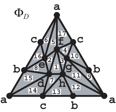
Figure 69: Relation $D$ and its Dowker complex $\Phi_{D}$. The complex is a triangulation of the Dunce Hat, a contractible space (the seemingly bounding edges actually touch, as suggested by the vertex labels). The Dunce Hat has no free faces, indicating that $D$ preserves attribute privacy.  (Vertices of $\Phi_{D}$ are attributes. Triangles are labeled with their generating individuals.)

Consider for example the relation $D$ of Figure 69. There are 17 individuals, each with three attributes. The figure also shows $\Phi_{D}$. We can see that there are no free faces, so the relation preserves attribute privacy by Lemma 62 on page 62. Moreover, each link $\mathop{\rm Lk}(\Psi_{D},x)$ is homotopic to a circle $\mathbb{S}^{1}$. Indeed, viewed from attribute space, that link is exactly the boundary of a triangle for each individual. Figure 70 shows such a link for individual #10. The link relation has a large number of individuals but only three attributes. So Theorem 10 holds and there is homology in the link. There is however no homology in the attribute complex of the relation $D$ itself; the simplicial complex $\Phi_{D}$ is a triangulation of the Dunce Hat, a nontrivially contractible space.

Although $R$ preserves attribute privacy, it does not preserve association privacy. For example: Individuals #1 and #12 share exactly one attribute (namely ${\tt h}$), but do so with four additional individuals (namely #3, #7, #11, and #13). If attributes represent shared dinners, then in some cases one can infer all the guests at a dinner after having seen as few as two guests. (Attribute privacy means that one cannot definitively infer additional dinners attended by a guest simply from having observed that guest at a particular dinner or two.)

$\begin{array}[]{c|ccc}Q&{\tt b}&{\tt c}&{\tt g}\\[2.0pt] \hline\cr 3&&&\bullet\\ 4&&\bullet&\bullet\\ 6&&\bullet&\\ 7&&\bullet&\\ 8&\bullet&&\\ 9&\bullet&&\bullet\\ 11&&&\bullet\\ 12&\bullet&&\\ 13&\bullet&\bullet&\\ 14&&\bullet&\\ 15&\bullet&&\\ 16&\bullet&\bullet&\\ 17&&\bullet&\\ \end{array}$

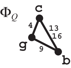
Figure 70: Relation $Q$ represents $\mathop{\rm Lk}(\Psi_{D},10)$ from Figure 69. Also shown is the attribute Dowker complex $\Phi_{Q}$. It is the boundary of a triangle, so homotopic to $\mathbb{S}^{1}=\mathbb{S}^{\kern 0.56001pt{k-2}}$. Since individual #10 has three attributes and $1=3-2$, that means relation $R$ preserves attribute privacy for individual #10. (Vertices of $\Phi_{Q}$ are attributes. Edges are labeled with their generating individuals. Notice that the edge $\{{\tt b},{\tt c}\}$ is generated by two individuals. Whereas most edges in $\Phi_{D}$ are shared by only two triangles, edge $\{{\tt b},{\tt c}\}$ is shared by three triangles; it is one of those edges that are glued to two others in the Dunce Hat representation. — Individuals who generate just vertices are not shown in the drawing of $\Phi_{Q}$ here.)

J.2 Disinformation

Privacy loss is possible when there is a free face in the relevant Dowker complex. One way to preserve privacy is to eliminate such free faces. Earlier in the report, we studied morphisms between relations as a possible way to transform data so as to reduce privacy loss. Ideally, for attribute privacy, the goal of such a transformation is to map onto a relation whose attribute complex has no free faces. We saw that such transformations need not always exist, for topological reasons, unless one is willing to introduce discontinuities, that is, discard knowledge of some relationships in the underlying spaces.

Alternatively, one could imagine embedding a relation within another that does preserve privacy. Of course, at the extreme, one simply embeds the given relation in a huge relation that looks like a perfect sphere. Now there is privacy but the same mechanism that provides privacy reduces utility. Nonetheless, one has not discarded relationships, merely surrounded them with disinformation. We saw an example of that early on, when we added a single attribute to relation $H$ in the example of Section 3.1, in order to remove the inference that someone had cancer. If one has a separate mechanism for discerning fake entries from legitimate entries, then one can see past the disinformation — in the earlier example that would entail having a (presumably safely encrypted) memory of which single entry in the relation is false.

$\begin{array}[]{c|ccccc}\hbox{\large$M$}&{\tt a}&{\tt b}&{\tt c}&{\tt d}&{\tt e}\\[2.0pt] \hline\cr 1&\bullet&\bullet&&&\bullet\\ 2&\bullet&\bullet&\bullet&&\\ 3&&\bullet&\bullet&\bullet&\\ 4&&&\bullet&\bullet&\bullet\\ 5&\bullet&&&\bullet&\bullet\\ \end{array}$

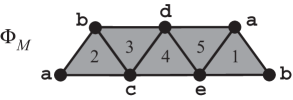
Figure 71: Relation $M$ revisited, along with its attribute complex $\Phi_{M}$.

Figure 71 revisits our earlier Möbius strip relation, showing the relation $M$ and its attribute complex $\Phi_{M}$. Loss of attribute privacy occurs when someone observes two attributes that form a free edge on the boundary of the Möbius strip, such as the edge $\{{\tt b},{\tt d}\}$. Given the relation, the observer can then infer a third attribute and identify the underlying individual, in this case infer attribute ${\tt c}$ and identify individual #3.

In order to preserve attribute privacy, one might consider adding decoy individuals whose so-called attributes include those edges, making the edges nonfree, thus removing that inference mechanism. Relation $MM$ in Figure 72 does so by doubling the number of individuals.

$\begin{array}[]{c|ccccc}\hbox{\large$MM$}&{\tt a}&{\tt b}&{\tt c}&{\tt d}&{\tt e}\\[2.0pt] \hline\cr 1&\bullet&\bullet&&&\bullet\\ 2&\bullet&\bullet&\bullet&&\\ 3&&\bullet&\bullet&\bullet&\\ 4&&&\bullet&\bullet&\bullet\\ 5&\bullet&&&\bullet&\bullet\\ 6&\bullet&\bullet&&\bullet&\\ 7&&\bullet&\bullet&&\bullet\\ 8&\bullet&&\bullet&\bullet&\\ 9&&\bullet&&\bullet&\bullet\\ 10&\bullet&&\bullet&&\bullet\\ \end{array}$

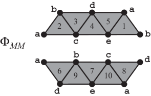
Figure 72: Relation $MM$ adds five decoy individuals. The attribute complex $\Phi_{MM}$ entails gluing two Möbius strips together.

The additional five individuals form their own Möbius strip. The figure therefore describes the overall attribute complex $\Phi_{MM}$ as two Möbius strips, with edges shared between the two strips, as suggested by the vertex labels. The overall attribute complex amounts to gluing the two Möbius strips together, boundary to zigzag spine. The resulting attribute complex is the 2-skeleton of the full complex on the attribute set $\{{\tt a},{\tt b},{\tt c},{\tt d},{\tt e}\}$. It therefore is homotopic to a wedge sum of four 2-spheres: $\mathbb{S}^{2}\vee\mathbb{S}^{2}\vee\mathbb{S}^{2}\vee\mathbb{S}^{2}$.

Each of $\Phi_{MM}$’s edges is now shared by three triangles. There are no free faces.

No attribute inference is possible.  (Association inference is possible.)

Moreover, the complex is sufficiently isotropic that one cannot say a priori  which individuals are real and which are decoys, even if one knows that there might be decoys. Of course, the curator of the relation likely would want some secure mechanism to separate truth from fiction, that is, to peel apart the gluing. Regardless, real individuals may be identified via $MM$ upon seeing all their attributes (and only then).

J.3 Insufficient Representation

In this subsection we show that if there are fewer than $2^{k}$ individuals in a nonvoid relation with $2k$ attributes that model $k$ bits for each individual, then the relation cannot preserve attribute privacy for everyone. The reason is that fewer than $2^{k}$ individuals amounts to removing some generating simplices from the potential attribute complex $\mathbb{S}^{\kern 0.56001pt{0}}*\mskip 2.0mu\mathbb{S}^{\kern 0.56001pt{0}}*\cdots*\mskip 2.0mu\mathbb{S}^{\kern 0.56001pt{0}}$, thereby creating free faces in $\Phi_{R}$. By similar intuition, it may be possible to preserve attribute privacy even if there are fewer than, say, $3^{k}$ individuals in a relation with $3k$ attributes representing $k$ trivalent pieces of information. After all, bits are a special case of tri-values, so one can preserve attribute privacy with certain $2^{k}$ individuals. Thinking simplicially, the potential attribute complex for tri-values is $(\mathbb{S}^{\kern 0.56001pt{0}}\vee\mskip 2.0mu\mathbb{S}^{\kern 0.56001pt{0}})*(\mathbb{S}^{\kern 0.56001pt{0}}\vee\mskip 2.0mu\mathbb{S}^{\kern 0.56001pt{0}})*\cdots*(\mathbb{S}^{\kern 0.56001pt{0}}\vee\mskip 2.0mu\mathbb{S}^{\kern 0.56001pt{0}})$. Removing some generating simplices from that space does not necessarily create free faces, as one can see by simple example.

Definition 102 (Binary Attribute Pair).

By a binary attribute pair we mean two mutually exclusive attributes, written $y$ and ${\overline{y}}$. No individual can have both attributes. Moreover, in what follows we will assume that every individual has exactly one attribute from any such pair.

Lemma 103 (Privacy Requires Many Individuals).

Suppose $Y=\{y_{1},{\overline{y}}_{1},y_{2},{\overline{y}}_{2},\ldots,y_{k},{\overline{y}}_{k}\}$, with $\,\{y_{i},{\overline{y}}_{i}\}$ a binary attribute pair, for $i=1,\ldots,k$, and $k\geq 1$.

Let $R$ be a relation on ${X}\mskip-1.8mu\times{Y}$, with $X\!\neq\emptyset$, such that every individual $x\in X$ has as attributes exactly one of $\{y_{i},{\overline{y}}_{i}\}$, for each $i=1,\ldots,k$.  Let $n$ be the number of distinct rows of $R$.

Then $R$ preserves attribute privacy if and only if $\hbox{\hskip 1.0pt}{}n=2^{k}$.

Proof.

Observe that each row of $R$ has exactly $k$ nonblank entries, so each maximal simplex of $\Phi_{R}$ consists of exactly $k$ vertices. Moreover, no row of $R$ is contained in another row unless the two rows are identical. We may therefore assume, without loss of generality, that all rows of $R$ are distinct and incomparable. Consequently, every $x\in X$ is uniquely identifiable. We can think of each individual $x\in X$ as defining a unique and identifying $k$-bit number, with one bit per binary attribute pair, as determined by that individual’s row, $Y_{x}$. All possible $k$-bit numbers are represented by $X$ if and only if $n=2^{k}$.

I. Suppose that $n=2^{k}$.

Showing that $\Phi_{R}$ contains no free faces would establish that $R$ preserves attribute privacy, by Lemma 62 on page 62. To show that $\Phi_{R}$ contains no free faces, it is enough to show that, for every maximal $\gamma\in\Phi_{R}$ and every $y\in\gamma$, the simplex $\gamma\setminus\{y\}$ is contained in some maximal simplex of $\Phi_{R}$ other than just $\gamma$.

Write $\chi=\gamma\setminus\{y\}$. Since $y$ is part of a binary attribute pair, we can construct a new set $\gamma^{\prime}$ from $\gamma$ by replacing $y$ with its “opposite”. Specifically: $\gamma^{\prime}=\chi\cup\{y_{i}\}$, if $y={\overline{y}}_{i}$; and $\gamma^{\prime}=\chi\cup\{{\overline{y}}_{i}\}$, if $y=y_{i}$. Since $n=2^{k}$, there is an $x\in X$ for which $Y_{x}=\gamma^{\prime}$. So $\gamma^{\prime}\in\Phi_{R}$, telling us $\chi$ is not free.

II. Suppose that that $R$ preserves attribute privacy.

By Lemma 63 on page 63, $\Phi_{R}$ contains no free faces.

Let $\gamma$ be a maximal simplex of $\Phi_{R}$ and $y\in\gamma$. Define $\chi=\gamma\setminus\{y\}$. Construct $\gamma^{\prime}$ as in part I above. Consider the collection $\Gamma={\left\{\eta\in\Phi_{R}\;\left|\;\chi\subsetneq\eta\right.\right\}}$. The only possible set that might be in $\Gamma$ besides $\gamma$ is $\gamma^{\prime}$. Since $\Phi_{R}$ contains no free faces, $\Gamma=\{\gamma,\gamma^{\prime}\}$.

Now vary $y$ across $\gamma$ and then repeat the process for all $\gamma^{\prime}$ thus constructed. The transitive closure of this process generates $2^{k}$ distinct maximal simplices in $\Phi_{R}$, each of which corresponds to a unique $x\in X$. So $n=2^{k}$. ∎

J.4 A Structural Inference Example: Passengers on Ferries

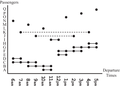
Figure 73: This time series represents 17 different passengers on 12 different ferry crossings. Each dot represents a passenger on a crossing. As a visual aid, solid lines connect multiple crossings by the same passenger at consecutive departure times, while dashed lines connect multiple crossings by the same passenger at non-consecutive departure times.

Imagine a commuter ferry that crosses back and forth between downtown and an island. Passengers pay electronically as they enter the ferry, so there is a record of who is on which crossing. Figure 73 shows a hypothetical time series for 12 crossings during a day in which 17 passengers took the ferry, some of whom crossed several times. Figure 74 shows the corresponding $\Psi_{R}$ complex: vertices are individuals; each triangle represents a particular crossing. (Each ferry crossing had three passengers in this simplified example.)

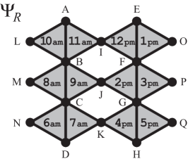
Figure 74: Simplicial complex $\Psi_{R}$ determined by viewing the time series of Figure 73 as a relation $R$. Vertices represent passengers, labeled with letters. Triangles represent ferry crossings, labeled with departure times.

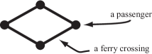
Figure 75: A waitress’s observations of passengers drinking coffee together at various times, represented by a simplicial complex. Vertices represent unknown but distinct passengers. Edges represent unknown but distinct crossing times.

The waitress in the ferry’s coffee shop observes four individuals ordering coffee and conversing during the day, appearing in pairs on four different crossings. She remembers seeing four distinct pairs, but does not remember the crossing times. Who are the individuals?

It is convenient to also represent the waitress’s observations as a simplicial complex. Figure 75 does so. Vertices are now the four unknown individuals; edges are their (unknown) common crossing times. One can interpret who the individuals are by embedding the complex of Figure 75 into the complex of Figure 74, using injective maps in both the passenger and time domains. There are exactly two such embeddings (modulo index permutations), given by the two ways one can wrap a rectangle around the two holes in the complex of Figure 74. (Those are the only two “diamonds” touching four different crossing times.) Thus the individuals are either $\{\hbox{C},\hbox{G},\hbox{J},\hbox{K}\}$ or $\{\hbox{B},\hbox{F},\hbox{I},\hbox{J}\}$, as indicated by Figure 76. Either way, one knows for sure that individual “J” twice had a conversation over coffee that day.

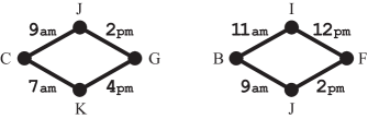
Figure 76: The two possible embeddings of the complex of Fig. 75 into the complex of Fig. 74.

Moreover, each of these embeddings places a time ordering on the embedded edges, from which one can make inferences as to who might have transmitted information to whom. For instance, for the embedding involving individuals $\{\hbox{B},\hbox{F},\hbox{I},\hbox{J}\}$, one sees that individual “J” could have been both the initial source and final recipient of information.

References

- [1] A. Björner. Topological methods. In R. L. Graham, M. Grötschel, and L. Lovász, editors, Handbook of Combinatorics, volume II, pages 1819–1872. Elsevier, Amsterdam, 1995.
- [2] I. Dinur and K. Nissim. Revealing information while preserving privacy. In Proceedings of the 22nd ACM Symposium on Principles of Database Systems, pages 202–210, 2003.
- [3] C. H. Dowker. Homology groups of relations. Annals of Mathematics, 56(1):84–95, 1952.
- [4] C. Dwork. Differential privacy: A survey of results. In Proceedings of the 5th International Conference on Theory and Applications of Models of Computation, pages 1–19, 2008.
- [5] C. Dwork. A firm foundation for private data analysis. Communications of the ACM, 54(1):86–95, 2011.
- [6] M. A. Erdmann. On the topology of discrete strategies. International Journal of Robotics Research, 29(7):855–896, 2010.
- [7] M. A. Erdmann. On the topology of discrete planning with uncertainty. In A. Zomorodian, editor, Advances in Applied and Computational Topology, pages 147–193. AMS, 2012.
- [8] Ú. Erlingsson, V. Pihur, and A. Korolova. RAPPOR: Randomized Aggregatable Privacy-Preserving Ordinal Response. In Proceedings of the 21st ACM Conference on Computer and Communications Security, pages 1054–1067, 2014.
- [9] R. Forman. A user’s guide to discrete Morse theory. Séminaire Lotharingien de Combinatoire, 48:B48c, 2002.
- [10] B. Ganter and R. Wille. Formal Concept Analysis: Mathematical Foundations. Springer-Verlag, Berlin, 1999.
- [11] R. Ghrist, D. Lipsky, J. Derenick, and A. Speranzon. Topological landmark-based navigation and mapping. Preprint, 2012.
- [12] P. M. Gleiser and L. Danon. Community structure in jazz. Advances in Complex Systems, 6(4):565–573, 2003.
- [13] F. Harary and R. Read. Is the null-graph a pointless concept? In Proceedings of the Capital Conference on Graph Theory and Combinatorics, pages 37–44, 1973.
- [14] A. Hatcher. Algebraic Topology. Cambridge University Press, Cambridge, 2002.
- [15] M. Hoang, R. Ramanathan, and A. Singh. Structure and evolution of missed collaborations in large networks. In The Sixth IEEE International Workshop on Network Science for Communication Networks, in conjunction with IEEE Infocom, pages 849–854, 2014.
- [16] J. R. Munkres. Elements of Algebraic Topology. Addison-Wesley, Menlo Park, CA, 1984.
- [17] A. Narayanan and V. Shmatikov. Robust de-anonymization of large sparse datasets. In Proceedings of the IEEE Symposium on Security and Privacy, pages 111–125, 2008.
- [18] D. Quillen. Higher algebraic K-theory: I. In Lecture Notes in Mathematics, volume 341, pages 85–147. Springer-Verlag, Berlin, 1973.
- [19] D. Quillen. Homotopy properties of the poset of nontrivial -subgroups of a group. Advances in Mathematics, 28(2):101–128, 1978.
- [20] J. J. Rotman. An Introduction to Algebraic Topology. Springer-Verlag, Berlin, 1988.
- [21] L. Sweeney. k-anonymity: A model for protecting privacy. International Journal of Uncertainty, Fuzziness and Knowledge-based Systems, 10(5):557–570, 2002.
- [22] M. L. Wachs. Poset Topology: Tools and Applications. IAS/Park City Mathematics Institute, Summer 2004. Also available here: http://arxiv.org/abs/math/0602226.
- [23] S. L. Warner. Randomized Response: A survey technique for eliminating evasive answer bias. Journal of the American Statistical Association, 60(309):63–69, 1965.
- [24] S. D. Warren and L. D. Brandeis. The right to privacy. Harvard Law Review, IV(5):193–220, 1890.
- [25] R. Wille. Concept lattices and conceptual knowledge systems. Computers & Mathematics with Applications, 23(6–9):493–515, 1992.