Study of anyon condensation and topological phase transitions from a topological phase using Projected Entangled Pair States
Abstract
We use Projected Entangled Pair States (PEPS) to study topological quantum phase transitions. The local description of topological order in the PEPS formalism allows us to set up order parameters which measure condensation and deconfinement of anyons, and serve as a substitute for conventional order parameters. We apply these order parameters, together with anyon-anyon correlation functions and some further probes, to characterize topological phases and phase transitions within a family of models based on a symmetry, which contains quantum double, toric code, double semion, and trivial phases. We find a diverse phase diagram which exhibits a variety of different phase transitions of both first and second order which we comprehensively characterize, including direct transitions between the toric code and the double semion phase.
I Introduction
Topological phases are exotic states of matter with a range of remarkable properties wen:book : They display ordering which cannot be identified by any kind of local order parameter and requires global entanglement properties to characterize it; they exibit strange excitations with unconventional statistics, termed anyons; and the physics at their edges displays anomalies which cannot exist in genuinely one-dimensional systems and thus must be backed up by the non-trivial order in the bulk. There has been steadily growing interest in the physics of these systems, both in order to obtain a full understanding of all possible phases of matter, to use their exotic properties in the design of novel materials, and to utilize tham a as a way to reliably store quantum information and quantum computations, exploiting the fact that the absence of local order parameters also makes their ground space insensitive to any kind of noise.
At the same time, the reasons which makes these system suitable for novel applications such as quantum memories also make them hard to understand, for instance when trying to classify and identify topological phases and study the nature of transitions between them. Landau theory, which uses local order parameters quantifying the breaking of symmetries to classify phases and describe transitions between them, cannot be applied here due to the lack of local order parameters. Rather, phases are distinguished by the way in which their entanglement organizes, and by the topological – this is, non-local – nature of their excitations. Formally, one can understand the relation of certain topological phases through a formalism called anyon condensation, which provides a way to derive one topological theory from another one by removing parts of the anyons by the mechanism of condensation and confinement bais2009condensate . While on a formal level, condensation should give rise to an order parameter, in analogy to other Bose-condensed systems such as the BCS state, it is unclear how to formally define such an order parameter in a way which would allow to use it to characterize topological phase transitions in a way analogous to Landau theory.
Tensor Network States, and in particular Projected Entangled Pair States (PEPS) verstraete:mbc-peps ; verstraete2004renormalization ; orus:tn-review , constitute a framework for the local description of correlated quantum systems based on their entanglement structure. It is based on a local tensor which carries both physical and entanglement degrees of freedom, and encodes the way in which these degrees of freedom are intertwined. This makes PEPS both a powerful numerical framework verstraete2004renormalization ; orus:tn-review , and a versatile toolbox for the analytical study on strongly correlated systems; in particular, they are capable of exactly describing a wide range of topological ordered systems verstraete:comp-power-of-peps ; buerschaper:stringnet-peps ; gu:stringnet-peps . In the last years, it has been successively understood where this remarkable expressive power of PEPS originates – this is, how it can be that topological order, a non-trivial global ordering in the systems’ entanglement, can be encoded locally in the PEPS description: The global entanglement ordering is encoded in local entanglement symmetries of the PEPS tensor, this is, symmetries imposing a non-trivial structure on the entanglement degrees of freedom. These symmetries ultimately build up all the topological information locally, such as topological sectors, excitations, their fusion and statistics 2010peps ; buerschaper:twisted-injectivity ; 214mpoinject ; bultinck:mpo-anyons . Recently, this formalism has been applied to study the behavior of topological excitations across phase transitions, and signatures of condensation and confinement had been identified haegeman2015shadows . Subsequently, this has been used to show how to construct order parameters for measuring condensation and deconfinement within PEPS wavefunctions, which in turn have allowed to build a mathematical formalism for understand and relating different topological phases within the PEPS framework through anyon condensation duivenvoorden:anyon-condensation . The core insight has been that the order parameters measuring the behavior of anyons within any topological phase are in correspondence to order parameters which classify the “entanglement phase” of the holographic boundary state which captures the entanglement properties (and in particular the entanglement spectrum) of the system.
In this paper, we apply the framework for anyon condensation within the PEPS formalism to perform an extensive numerical study of topological phases and phase transitions within a rich family of tensor network models. The family is based on PEPS tensors with a symmetry, with the quantum double model as the fixed point, and correspondingly types of anyons. Within this framework, we find a rich phase diagram including two different types of topological phases, the Toric Code model and the Double Semion model, which are both obtained through anyon condensation from the model, as well as trivial phases. The phase diagram we find exhibits transitions between all these phases, including direct transitions between the TC and DS model which cannot be described by anyon condensation.
Based on the understanding of anyon condensation within tensor networks, we introduce order parameters for anyon condensation and deconfinement, as well as ways of extracting correlation functions between pairs of anyons, which allows us to characterize the different topological phases and the transitions between them in terms of order parameters and correlation functions, and to study their behavior and critical scaling in the vicinity of phase transitions. Using these probes, we comprehensively explore the phase diagram of the above family of topological models, and find a rich structure exhibiting both first and second order phase transitions, with transition lying in a number of different universality classes, including a class of transitions with continuously varying critical exponents. In particular, we find that the transition between Double Semion and Toric Code phases can be both first and second order, and can exhibit different critical exponents, depending on the interpolating path chosen.
The paper is organized as follows. In Sec. II, we introduce tensor networks and the concepts relevant to topological order, anyonic excitations, and anyon order parameters. We then introduce the family of topological models based on -invariant tensors which we study in this work: We start in Sec. III by introducing the corresponding fixed point models and discussing their symmetry patterns, and proceed in Sec. IV to describe the ways in which we generate a family of models containing all those fixed points. In Sec. V, we give a detailed account of the different numerical probes we use for studying the different phases and their transitions, and discuss how they can be used to identify the nature of a transition. In Sec. VI, we then apply these tools to map out the phase diagram of the families introduced in Sec. IV and comprehensively study the transitions between them. The results are summarized in Sec. VII.
II Tensor network formalism and quantum doubles
In this section, we introduce PEPS and give an overview of the relevant concepts and notions which appear in the description of topological phases with tensor networks, with a special focus on quantum doubles and phases obtained from there by anyon condensation. We will show how these ideas are connected and later we will use them for our study of topological phases and phase transitions.
II.1 Tensor network descriptions
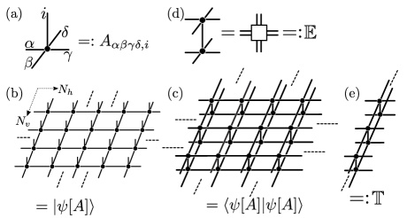
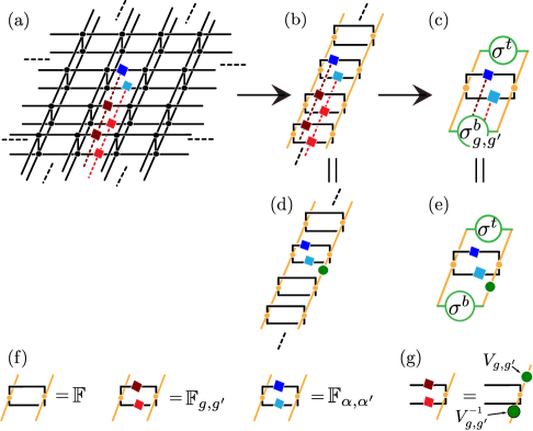
PEPS describe a many body wavefunction in terms of an on-site tensor (Fig. 1a). Here, the Roman letter denotes the physical degree of freedom at a given site, while the Greek letters denote the so-called virtual indices or entanglement degrees of freedom used to build the wavefunction. The many-body wavefunction is then constructed by arranging the tensors in a 2D grid, as shown in Fig. 1b, and contracting the connected virtual indices, i.e., identifying and summing them. This construction applies both to systems with periodic boundaries, to infinite planes, and to semi-infinite cylinders.
Given a description of a many body wavefunction in terms of a local tensor (Fig. 1b), the computation of the expectation value of local observables and the norm of wavefunctions can be reduced to a tensor network contraction problem, see Fig. 1c. We will now systematically discuss the objects which appear in the course of this contraction. The contraction of the physical indices of a single tensor and its conjugate leads to the tensor , Fig. 1d, which we refer to as the on-site transfer operator. It can be interpreted as a map between virtual spaces in the ket and bra layer. By contracting one row or column of , we arrive at the transfer operator , Fig. 1e. It mediates any kind of order and correlations in the system, and it will be an object of fundamental importance for our studies. More details on transfer operators will be discussed in Sec. II.5.
II.2 Virtual symmetries and QD
Symmetries of the virtual indices, or briefly virtual symmetries, play a crucial role in the characterization of the topological order carried by a PEPS wavefunction 2010peps ; buerschaper:twisted-injectivity ; 214mpoinject . Virtual symmetries are characterized by the invariance under an action on the virtual indices of tensor . More precisely, is called -invariant if one can pull through the action of on the virtual legs of ,
| (1) |
where the red squares represent a unitary group action , , with a (faithful) representation of , this is,
We can alternatively consider as a map from virtual to the physical space, in which case (1) states that is supported on the -invariant subspace, i.e., the subspace invariant under the group action . If this map is moreover injective on the -invariant subspace, it is called -injective; and if it is an isometry, -isometric.
A specific case of interest is given by -isometric tensors, since they naturally provide a description of the ground space of the so-called quantum double (QD) models of Kitaev kitaev2003fault . A -isometric tensor can be constructed by averaging over the group action of :
| (2) |
up to normalization (which we typically omit in the following), where , with the generator of the regular representation of .
II.3 Anyonic excitations of the QD
The anyonic excitations of the QD are labeled by group elements (fluxes) and irreducible representations (irreps) of kitaev2003fault . Starting from a tensor network description of the ground state (anyonic vacuum), such an anyonic excitation can be constructed by placing a string of ’s along the virtual degrees of freedom of the PEPS, and terminating it with an endpoint which transforms like an irrep of , for instance or 2010peps (both of which we will use later on). A state with one such anyon thus looks like
| (3) |
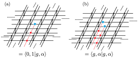
where the red squares on the red string denote the group action (flux) and the blue square represents the irrep endpoint (charge), which in our case will be always chosen as . By virtue of Eq. (1), the (red) string of can be freely deformed, and thus, only its endpoint can be observed and forms an excitation. Excitations with trivial are termed fluxes, while those without string () are termed charges, and excitations with both non-trivial and are called dyons. The statistics of the excitations is determined by the commutation relation of fluxes and charges, . In a slight abuse of notation, we will denote both the state with an anyon and the anyon itself by . Also, we will denote the vacuum state by .
In principle, such excitations need to come in pairs or tuples with trivial total flux and charge: On a torus, this is evident since strings cannot just terminate and the overall irrep must be trivial; with open boundaries, the boundary conditions must compensate the topological quantum numbers of the anyons and thus cannot be properly normalized with respect to the vacuum unless the total flux and charge are trivial. However, since we can place the anyons very far from each other, and we assume the system to be gapped (i.e., have exponentially decaying correlations), there is no interaction between the anyons, and their behavior (in particular the order parameters introduced in the next section) factorize. It is most convenient to construct a state with trivial total flux and charge by (i) using only anyons of the same type – this way, we can uniquely assign a value of the order parameter to a single anyon (in principle, only their product is known) – and (ii) arranging them along a column at large distance, which allows to map the problem to boundary phases, as explained in Sec. II.5. Let us add that since the numerical methods employed in this work explicitly break any symmetry related to long-range correlations between pairs of distant anyons, any such expectation value can be evaluated for a single anyon (cf. Sec. V.1).
II.4 Condensation and deconfinement fractions
We have seen that anyonic excitations in a -isometric PEPS can be modeled by strings of group actions with dressed endpoints. Remarkably, while describing pairs of physical anyons, these string operators act solely on the entanglement degrees of freedom in the tensor network. They continue to describe anyonic excitations when deforming the tensor away from the -isometric point by acting with an invertible operation on the physical indices (thus preserving -invariance), without the need to “fatten” the strings as it were the case for the physical string operator which create anyon pairs. However, if the deformation becomes too large, the topological order in the model must eventually change, even though the deformation still does not affect the string operators which describe the anyons of the QD phase. However, as different topological phases are characterized by different anyonic excitations, there must be a change in the way in which these virtual strings correspond to physical excitations. The mechanisms underlying these phase transitions is formed by the closely related phenomena of anyon condensation and anyon confinement bais2009condensate . In the following, we briefly review the two concepts in the context of tensor networks, with a particular focus on how to use the tensor network formalism to derive order parameters for topological phase transitions. A rigorous and detailed account of these ideas in the context of tensor networks is given in Ref. duivenvoorden:anyon-condensation .
Condensation describes the process where an anyonic excitation becomes part of the (new) vacuum, this is, it does no longer describe an excitation in a different topological sector than the vacuum. More precisely, we say an anyon has been condensed to the vacuum if
| (4) |
The phenomenon dual to condensation is confinement of anyons; indeed, condensation of an anyon implies confinement of all anyons which braid non-trivially with it bais2009condensate ; duivenvoorden:anyon-condensation . When separating a pair of confined anyons, their normalization goes exponentially to zero, and thus, an isolated anyon which is confined has norm zero. Within PEPS, we thus say that an anyon is confined if
| (5) |
again with the notation of Fig. 2b.
Condensation and confinement of anyons play a crucial role in characterizing the relation of different topological phase. Within a given symmetry, any topological phase can be understood as being obtained from the QD through condensation of specific anyons, and is thus characterized by its distinct anyon condensation and confinement pattern bais2009condensate ; duivenvoorden:anyon-condensation . In order to further study the transition between different topological phases, we can generalize the above criteria Eqs. (4) and (5) for condensation and confinement to order parameters, measuring the
and the
respectively. These constitute non-local order parameters for topological phases, which can therefore be used as probes to characterize topological phase transitions and their universal behavior, in complete analogy to conventional order parameters in Landau theory. The most general quantity of interest which we will consider, encompassing both condensation and deconfinement fractions, will thus be the overlaps of wavefunctions describing two arbitary anyons, with condensate and deconfinement fractions as special cases. Note that as of the discussion in the preceding section, is only determined up to a phase, and we will choose it to be positive.
II.5 Boundary phases and string order parameters
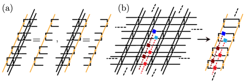
The behavior of condensate and deconfinement fractions is closely related to the phases encountered at the boundary of the system, this is, in the fixed point of the transfer operator duivenvoorden:anyon-condensation . To understand this relation, consider a left and right fixed point and of , see Fig 3a. Then, any such order parameter for the behavior of anyons can be mapped to the evaluation of the corresponding anyonic string operator – this is, a string and irreps in ket and bra indices – inbetween and , see Fig. 3b. (If the fixed point is not unique, and have to match; in our case, this is easily taken care of since is hermitian.) Since inherits a symmetry from the tensor, an irrep serves as an order parameter which detects breaking of the symmetry. The numerical methods we use will always choose to break symmetries when possible, which explains why it is sufficient to consider a single anyon (rather than a pair of anyonic operators, which would also detect long-range order without explicit symmetry breaking.) Similarly, strings create domain walls in the case of a broken symmetry, and thus detect unbroken symmetries. Finally, combinations of irreps and strings form string order parameters, which detect non-trivial symmetry protected (SPT) phases of unbroken symmetries.
We thus see that the behavior of anyonic order parameters is in direct correspondence to the phase of the fixed points of the transfer operator under its symmetry – this is, its symmetry breaking pattern and possibly SPT order – as long as these fixed points are described by short-range correlated states (as is expected in gapped phases). Specifically, in the case of the fixed point tensors which we discuss in the next section, the fixed points are themselves MPS, and we will be able to determine their SPT order and the behavior of the anyonic order parameters analytically.
III Topological phases: Fixed points
We now describe the tensor network constructions for the renormalization group (RG) fixed points of topological phases which can be realized by -invariant tensors. The form of the local tensor which we use for describing the RG fixed point of a topological phase is motivated by the desired symmetry properties of its transfer operator fixed points, and from the given tensors, we explicitly derive the fixed points of the transfer operator. Furthermore, we discuss the condensation and confinement pattern of anyons in each of those topological phases.
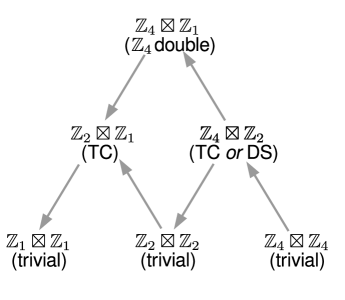
The different topological phases which can be realized in the case of -invariant tensors, and the corresponding symmetry breaking patterns, have been studied in Ref. duivenvoorden:anyon-condensation . For the case of -invariant tensors, the different phases and the symmetry of their transfer operator fixed points are given in Fig. 4, where the notation denotes a diagonal symmetry (this is, acting identically on ket and bra) and an off-diagonal symmetry (this is, acting on one index alone). For example, is generated by the diagonal element and the off-diagonal element .
III.1 quantum double
The quantum double (QD) is a topological model which can be realized by placing -level states on the oriented edges of a square lattice and enforcing Gauss’ law at each vertex,
| (6) |
the QD is then obtained as the uniform superposition over all such configurations. A tensor network description of QD is given by a -isometric tensor as defined in Eq. (2). We begin by writing down the on-site tensor (Fig. 1a) for the ground state of QD as a Matrix Product Operator (MPO):
| (7) |
and . Here, the inner indices jointly correspond to the physical index of the on-site tensor, and the outside indices to the virtual indices. Empty circles denotes the hermitian conjugate (with respect to the physical+virtual indices).
The relation of the construction Eq. (7) with the double model can be understood by considering in its diagonal (irrep) basis. Then, any entry of the on-site tensor is non-zero precisely if Eq. (6) is satisfied, i.e.,
| (8) |
where , which after contraction yields precisely the equal weight superposition of all configurations satisfying the Gauss law [Eq. (6)], and thus the wavefunction of the model.
Now, let us construct the fixed points of the transfer operator. First, note that with the properly chosen normalization factor, the MPO in (7), as a map from outside to inside, is a hermitian projector. (Here and in what follows, all such statements will be up to normalization.) Thus, the on-site transfer operator, Fig. 1d, is again of the form (7). The fixed points of the transfer operator and their symmetry properties can be deduced by using the following property of MPO tensors:
| (9) |
where the object on the right denotes a -tensor (i.e., it is if all indices are equal, and otherwise). Using Eq. (9), we can write the transfer operator as
| (10) |
where the top/bottom indices denote both the ket and bra indices [this is, the inside and outside indices of Eq. (7)]. The -tensors between adjacent sites force the indices in the loops to be equal, and thus the transfer operator can be written as a sum over four product operators,
| (11) |
The fixed points of this transfer operator are then the following four product states:
| (12) |
since . Each of the fixed points of the transfer operator in (12) breaks the symmetry of the transfer operator down to , since they are invariant under the diagonal action on the bra and ket index, but get cyclically permuted by the off-diagonal action . It should be noted that this symmetry breaking structure directly originates from the block structure of the on-site transfer operator [which is the same as Eq. (7)], where each of the ket/bra leg pairs is simultaneously in the state for .
The behavior of operators which act trivially (up to a phase factor) on the fixed points of the transfer operator can be understood by their action on the local tensors describing the fixed point space, which are again of the form , as in Eq. (7). For each symmetry broken fixed point, the fixed point MPO (cf. Fig. 3a) is thus of the form
| (13) |
with a trivial MPO bond dimension (yellow) , where is an additional phase factor whose exact value depend on the specific fixed point as well as the charge label . We now see that any symmetry action with , as well as any irrep action with , leave the fixed point invariant (up to a phase). On the other hand, acting with either or on the fixed point yields a locally orthogonal tensor, as can be either computed explicitly from Eq. (12) or inferred from the commutation relations with Eq. (13). We thus arrive at
This is, no anyon is condensed, and all anyons are deconfined, and we have a model with the full anyon content, as expected.
III.2 Toric Codes
Next, we will discuss how to construct Toric Codes (TC), i.e., double models, starting from the tensor of the model, while keeping the symmetry of the tensor. We will do so by acting with certain projections on the physical indices, which reduce or enhance the symmetry of the transfer operator fixed points of the model to and , respectively, and which yield two Toric Codes which are related by an electric-magnetic duality buerschaper2013electric .
III.2.1 Toric Code
Let us first show that by acting with the projector on the local tensors of the QD, we obtain a tensor for the RG fixed point of the TC phase where the fixed points of the transfer operator have a symmetry. The new tensor is obtained from (7) as
| (14) |
The action of the projections, denoted by red dots, on the black ring (i.e., the tensor) gives two independent blocks, and the resulting tensor can be written as an MPO with bond dimension two:
| (15) |
and . The reason why Eq. (15) provides a tensor network description for the Toric Code can be understood from the equivalence
| (16) |
where and is the generator of . Up to the , it is thus exactly of the same form as (7), but with the underlying group , and thus describes a model (i.e., the Toric Code). The construction of Eq. (15) can therefore be viewed as a model, tensored with an ancilla qubit in the state.
The on-site transfer operator of this model again satisfies the delta relation of Eq. (9) (now with only two possible values), and each of the two blocks in Eq. (15) can be identified with a symmetry broken fixed point of the transfer operator, which are thus of the form
| (17) |
Each of the fixed points is invariant under the action of and , while transforms between them. We thus find that the Toric Code model at hand has a symmetry in the fixed point of the transfer operator, and we thus henceforth call it the Toric Code.
Graphically, the actions which leave fixed points invariant can be summarized as follows
| (18) |
where is a phase factor with a value which depends on the fixed point, while all other actions yields locally orthogonal tensors. We can thus summarize the condensation and confinement pattern of anyons at the RG fixed point of TC phase as
This implies that the anyon is condensed, while the anyons with have become confined, giving rise to a TC with anyons , , and (the fermion).
III.2.2 Toric Code
A second construction for a TC phase in the framework of -invariant tensors is obtained by a dual projection. We will see that this projection, in contrast to the TC, reduces the symmetry of fixed points of the transfer operator to , and the fixed point space of the transfer operator is spanned by eight symmetry broken fixed points. The projection action on the physical indices is given by , and, acting on the QD tensor, generates an MPO with eight blocks,
| (19) |
, and . Together with the index of the other ring, Eq. (7), the bond dimension around the circle is .
It can be checked directly that (19) is again a hermitian projector, and that the on-site transfer operator satisfies a delta relation as in Eq. (9). Thus, we find that the fixed points of the transfer operator are
| (20) |
where and . They are invariant under , while any other symmetry action results in a permutation action on the fixed points. We thus find that the symmetry of the fixed point space is given by . The set of all symmetries of the fixed point tensor is thus given by
| (21) |
while all other actions with or give rise to orthogonal tensors. The overlap of anyonic wavefunctions is thus
This implies that is condensed, while the anyons with and are confined. The anyons of the TC are thus give by , , and (the fermion).
III.3 Double semion model
A model closely related to the TC is the double semion (DS) model. It also corresponds to a loop model, but is twisted with a -cocycle which assigns an amplitude to loop configurations with loops. It has no tensor network description in terms of -invariant tensors, and its description either requires -invariance iqbal2014semionic , or tensors which are injective with respect to MPO-symmetries 214mpoinject . As we will see, the fixed points of the transfer operator of the DS model also have a symmetry duivenvoorden:anyon-condensation , but they realize a different phase under that symmetry as compared to the TC, which is characterized by a non-zero string order parameter (i.e., an SPT phase), corresponding to the fact that it is obtained by condensing a dyon (a composite charge-flux particle) in the model. The local tensor of the DS model can be constructed by applying the following MPO projector (green) on the QD,
| (22) |
with ; arrows in the ring point in the direction of index . While it can be shown that this PEPS can be transformed to the QD model by local unitaries duivenvoorden:anyon-condensation , we will instead directly derive the fixed points of the transfer operator and show that they exhibit the symmetry pattern required for the DS phase. The composition of the QD (black ring) and DS (green ring) projector can be simplified to
| (23) |
where the index is identical on the top and bottom leg. (Here, we have used a redundancy in the description which allows to restrict to , and removed phases which cancel out between adjacent tensors.)
As in the previous cases, the tensor (22) is a hermitian projector. Connecting two tensors (in the form (23)] as required for the transfer operator, cf. Eq. (9), yet again gives rise to a tensor for all three indices , , and . The fixed points are thus given by MPOs with tensors of the form
| (24) |
where labels the two fixed points, and the green line is the MPO index for the fixed point MPO, with .
From (24), it can be seen that the symmetry actions which leave the tensor invariant are
| (25) |
while permutes the two fixed points, and maps it to a locally orthogonal tensor. It follows that the fixed point has symmetry, which is however not detected by local order parameters, but requires the use of string order parameters. The non-vanishing string order parameters can be read off Eq. (25): On the one hand, this is with a string of going downwards, and on the other hand, with a string of going downwards. It is crucial to notice that here, we have to fix the direction in which the string is pointing (since the virtual actions of the irreps are asymetric), and in the latter case, the endpoint has to be “dressed” by using as an irrep. This effectively moves the virtual action to the lower leg; otherwise, the string order parameter would vanish even though it were allowed for topological reasons, i.e., from the combination of group action and irrep it carries.
This leads us to adapt the definition of the anyons, cf. Eq. (3), used in this work by choosing irrep endpoints and for anyons with a string or , i.e., and , while using as endpoints for all other anyons. Importantly, the results on the former phases (and the trivial phases described later) still hold with these modified anyons. In fact, the only other phase where these anyons are not confined – in which case string operators involving them yield zero for topological reasons, i.e., solely due to the choice of group element and irrep of the string duivenvoorden:anyon-condensation – is the model, in which case it can be easily checked that the modified anyons are still uncondensed and deconfined.
The presence of string order with respect to the order parameters for the unbroken symmetry implies that the fixed point states describe a non-trivial SPT phase with symmetry . Using Eq. (25), we find
This shows that in the DS phase, only the dyon is condensed. The anyons with even and , as well as odd and , are condensed. The semions of the model are and , and the boson is .
III.4 Topologically trivial phases
Let us finally discuss how to obtain topologically trivial phases (TP) from the model. We will find that there are three different ways of obtaining such models, distinguished by their condensation/confinement pattern.
III.4.1 trivial phase
The first trivial phase is obtained by applying a projector ,
| (26) |
to the physical indices of the QD, which projects each of the indices indiviually on the trivial irrep. Clearly, this commutes with the symmetry action of the projector, Eq. (7), and thus, the on-site transfer operator itself is of the form , which in turn implies that the fixed point of the transfer operator is unique, and of the form as well. The model thus has symmetry at the boundary. A manifestation of this symmetry is the condensation of all the flux anyons, and correspondingly confinement of all charged particles. The condensation and confinement properties of anyons in the TP can be summarized as
III.4.2 trivial phase
The second trivial phase is obtained by applying an MPO projector (brown) to the projector as follows:
| (27) |
where . Combining it with the projector with tensor , we find that can be restricted to , and (27) yields again a hermitian projector. Contraction of adjacent on-site transfer operators yields yet again a Kronecker delta on the two loop variables, leading to four fixed points of the form
| (28) |
It is immediate to see that these are invariant under , and are permuted by and (acting on and , respectively). Thus, this phase has symmetry . Overall, this yields
Anyons with and are condensed, while anyons with or are confined, making the anyon content trivial.
III.4.3 trivial phase
The last trivial phase is obtained by acting on the with an MPO projector with bond dimension ,
| (29) |
where . The effective MPO which is obtained by composing black and violet rings has bond dimension , with tensor elements . It is thus clearly a hermitian projector, and has fixed points of the form which clearly break all symmetries, giving rise to a symmetry of the fixed point. The phase is trivial with all charges condensed and thus all anyons with non-trivial flux (including dyons) confined,
IV Topological phases: Interpolations and transitions
The fixed point tensors discussed in the preceding section all share the -invariance as a common feature. It is therefore suggestive to try to build smooth interpolations within these tensors, e.g. by starting from the -isometric tensor and deforming it smoothly towards some other fixed point model. As long as this deformation is reversible (as will be the case here), it corresponds to a smooth deformation of the parent Hamiltonian schuch:mps-phases , and thus forms a tool to study the phase diagram of the corresponding model. Since, as we have discussed in the previous section, the different phases are characterized by different symmetries at the boundary and thus different anyon condensation patterns, this will give rise to topological phase transitions which are (potentially) driven by anyon condensation.
In the following, we will discuss a number of interpolations which allow us to study all the phases in Fig. 4. The interpolations are obtained using two different recipes: The first approach aims to interpolate between the on-site tensors of the respective models in an as local as possible way; we will refer to this approach as local filtering. The second approach is based on interpolating between the on-site transfer operators rather than the tensors, which however can be shown to correspond to a smooth path of tensors due to some positivity condition; we will refer to it as direct interpolation of transfer operator.
The interpolations described in the following, and in particular the nature of the phase transitions, will be studied numerically in Sections V and VI.
IV.1 Three-parameter family with all topological phases
We start by describing a three-parameter family which exhibits all four topological phases in Fig. 4, together with the trivial phase. To start with, we define the following three one-parameter interpolations.
Third,
| (32) |
and . At , , and whole ring acts trivially, whereas for , , and the green ring acts as the DS projector, Eq. (22).
It is straightforward to verify that all three deformations (30–32) commute both among each other and with the projector. We can thus combine them to obtain a three-parameter tensor
| (33) |
which is parametrized by . From the mutual commutation, it follows that the limits , , and still yield the corresponding fixed point models, and the model. Finally, it is straightforward to check that by setting any two of the , we obtain the trivial phase.
IV.2 Transitions into trivial phases
The three-parameter family of the previous section did not include all the trivial phases present in Fig. 4. We now give three families interpolating from each of the different topological phases to the trivial ones.
IV.2.1 TC and trivial phases
The TC can be deformed into or TP through the two-parameter family
| (34) |
, and where the black ring represents the local tensor of the QD. It is built such as to interpolate between the tensors (14), (26), and (27) of the respective fixed point models: For , it gives the TC, for the TP, and for the TP.
IV.2.2 TC and trivial phases
IV.2.3 DS and trivial phases
Finally, we describe an interpolation which connects the DS and the TP and TP:
| (36) |
, and where with the Pauli matrix. Its extremal points are at the DS model, at the TP, and at the TP. Moreover, the point realizes the model. As we will see in Sec. VI.5, there exists a direct path between DS and TP via a multi-critical point.
IV.3 Direct interpolation of transfer operator
Let us now describe our second approach to constructing interpolations, the direct interpolation of the transfer operator. While they in principle form a special case of local filtering operations, the idea here is to construct an interpolation on the level of the on-site transfer operators, rather than the tensor, which yields different interpolation paths and in some cases seems to be more robust in retrieving direct phase transitions between the involved phases.
We start from two on-site tensors and which form the RG fixed point of two distinct phases. We assume that and are both -invariant, i.e., they can be obtained by applying linear maps on the local tensor of the QD, i.e., , where denotes the on-site tensor of the QD.
Now consider a direct interpolation of the on-site transfer operators ,
| (37) |
. Since , it follows that also , and thus for some ; moreover, can be chosen continuous in . In the case where the are commuting hermitian projectors, a continuous can be constructed through
| (38) |
where .
We will use this construction in three cases: (i) In Sec. V, we will use it to interpolate between the DS to TC model, i.e., and are the DS and TC projectors of Eqs. (22) and (15). (ii) Also in Sec. V, we will use it to interpolate between the QD and the TC. Here, is trivial, and the same as before. (iii) Finally, in Sec. VI.3.2, we will use it to interpolate between the DS and the TC model, with and from Eqs. (22) and (19). In all these cases, and commute, as we have seen in Sec. IV.1.
V Numerics: Methods
We will now give an overview over the numerical tools and methods which we will use to probe the phase diagram and in particular the phase transitions between different topological phases. Most impartantly, these are order parameters for condensation and deconfinement, as well as different correlation lengths (including those corresponding to anyon-anyon correlation functions involving string operators). We will also discuss a few additional probes suitable to characterize phase transitions. We will both describe the corresponding probes, and give detailed account of how to compute them.
In order to better illustrate how these probes can be used to characterize phase transitions, and to show how to use them to distinguish first-order from second-order phase transitions, we will study two specific interpolations, namely DS TC and QD TC. Both of these interpolations are constructed by linear interpolation of the on-site transfer operators as explained in Sec. IV.3.
V.1 Order parameters
Order parameters play a fundamental role in characterizing the nature of phase transitions, and are at the heart of Landau’s theory of second order phase transitions. Their behavior allows to identify different phases through their symmetry breaking pattern, to distinguish first from second order phase transitions, and to further characterize second order transitions through their critical exponents. While topological phases do not exhibit local order parameters, we have seen in Sec. II.4 and II.5 how to define order parameters for anyon condensation and deconfinement through operators defined on the virtual, i.e., entanglement degrees of freedom. In the following, we discuss how these order parameters can be measured, and how they can be used to characterize the nature of topological phase transitions.
V.1.1 Computation
As explained in Sec. II.4, any possible such order parameter is given by an anyonic wavefunction overlap (normalized by ), shown in Fig. 5a. Here, the strings (red) and their endpoints (blue) correspond to group actions , and irrep actions and , respectively. To compute this quantity, we proceed in two steps: In a first step, we approximate the the left and right fixed points of the transfer operator by Matrix Product Operators. This reduces the (2D) computation of to evaluating a (1D) string-order parameter in the left and right fixed point, Fig. 5b, which is then carried out in a second step (cf. also Sec. II.5).
The computation of the left and right fixed points and of the transfer operator in the thermodynamic limit is carried out using a standard infinite matrix product state (iMPS) algorithm. The basic idea is to use an infinite translational invariant MPS ansatz with some bond dimension to approximate the fixed point. This ansatz can e.g. be optimized by a fixed point method, this is, by repeatedly applying the transfer operator to it (this increases the bond dimension which is truncated to in every step by keeping the terms with the highest Schmidt coefficients, and is the method used in this paper), or in the case of a hermitian transfer operator by variationally optimizing the iMPS tensor, e.g. by linearizing the problem, until convergence is reached. A detailed overview over different methods for finding fixed points of transfer operators can be found in Ref. haegeman:medley . In all cases, truncating the bond dimension to a finite value induces some error, and therefore, an extrapolation in is required. An important point about all these methods is that they will favor symmetry broken fixed points – this is, whenever the fixed point is degenerate, the method will pick a symmetry broken fixed point rather than a cat-like state with long-range order, as the former has less correlations. As already discussed earlier, this is the reason why we can evaluate anyonic order parameters by considering just a single anyon (which requires symmetry breaking to be non-zero) rather than a distant pair of anyons (which would also detect long-range order in cat-like fixed points).
We have now rephrased the computation of in terms of a string order parameter evaluated in and , as shown in Fig. 5b; this has to be normalized by evaluating the same object without the string order parameter, i.e., . In both cases, we have to evaluate an object of the form Fig. 5b. This can be carried out by considering the transfer operators from top and bottom in Fig. 5b, which we will term channel operators, shown in Fig. 5f: is obtained by contracting the “physical” indices of the local MPO tensors of and , carries additional group actions and indicated by the red squares, and carries the irrep actions (blue) which correspond to the desired anyon. First, we must compare the modulus of the leading eigenvalue of with the leading eigenvalue of : If the former is strictly smaller, will be exponentially supressed in the length of the string, and thus be zero. This is the case exactly if the symmetry is broken, since the normalized leading eigenvalue determines the overlap of the original and the symmetry-transformed fixed point per unit cell. In case the symmetry is unbroken, we compute the largest eigenvector of from the bottom and the largest eigenvector of from the top by exact diagonalization. (Note that the eigenvectors are unique, since the fixed point iMPS will break symmetries, and are unbroken symmetries – a degenerate eigenvector would indicate long-range order.) Finally, the expectation value is computed by acting on with and from the top and bottom respectively as shown in Fig. 5c.
However, there is an important issue: We still have to fix normalization, as the eigenvectors have no well-defined normalization. To this end, we note that since we only consider unbroken symmetries , the symmetry is locally represented in the fixed point iMPS through some action and , as shown in Fig. 5g sanz:mps-syms . By suitable rescaling , we can always choose to be a representation, and it will be crucial that we do so. We now substitute Fig. 5g everywhere in Fig. 5b and obtain the expression Fig. 5d for the fraction , which simplifies to the expression Fig. 5e with the same and as in the normalization (which has and .) In order to fix the normalization we can thus either extract the symmetry action from the iMPS fixed point through and evaluate Fig. 5e, or we can choose a canonical gauge for the iMPS of such that the symmetry action is unitary 111This is the case for both a right- or a left-canonical gauge for , this is, the gauge where either the right or the left fixed point of the transfer operator of the iMPS representing alone is the identity., and normalize and with a unitarily invariant norm, e.g. .
It is important to note that this choice of normalization – which hinges upon the choice of – is not arbitrary. First, the result is invariant under changing the gauge of the iMPS for and . Second, normalizing such as to form a representation is necessary to obtain the same value for each anyon when aligning several identical anyons along a column (with their strings in parallel): Otherwise, the contribution of some of the anyons will be given Fig. 5e with as the green dot, while for others it will be , which is only guaranteed to give the same result if the form a representation.
V.1.2 Analysis
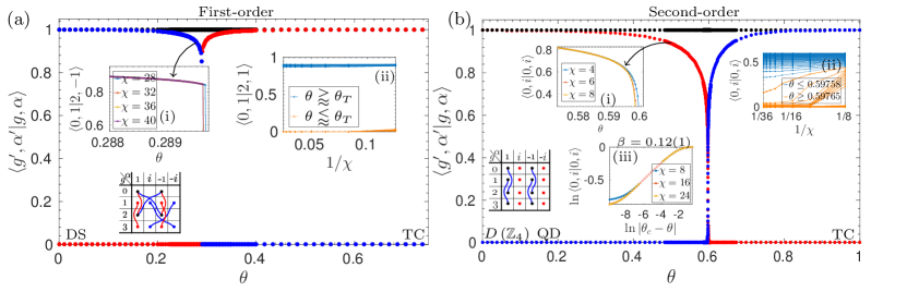
Let us now analyze the behavior of anyonic order parameters in the case of the two interpolations DS TC and QD TC, shown in Fig. 6a and b, respectively. Since there are anyons ( and can each take four possible values), there are in total different overlaps. However, it turns out that many of these overlaps are either zero, in which case we omit them from the figure, or equal to each other (this can both be observed numerically and explained from the symmetry structure of the state). The main plots in Fig. 6a,b show the remaining different non-zero order parameters. The color coding in any such plot is explained in the table in the lower left corner: The boxes in the table correspond to different anyons (rows label , columns label ). The colors of the dots and lines in the table correspond to the different non-zero order parameters: Solid dots represents the norm , and lines between two entries represents overlaps , where and . The absence of a dot or an edge indicates quanitites which remain zero along the whole interpolation, this is, each such plot carries the full information on all .
Specifically, in Fig. 6a, the blue curve describes both the condensate fraction of and the deconfinement fraction of the anyon with , while the red curve describes the condensate fraction of and deconfinement fraction of ; this relates to the fact that at the DS–TC transition, particles have to both condense/confine and uncondense/deconfine. In Fig. 6b, the blue curve gives the condensate fraction of and the red one the deconfinement fraction of : At the phase transition into the TC phase, the former condensed and the latter becomes confined.
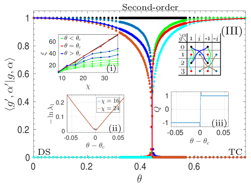
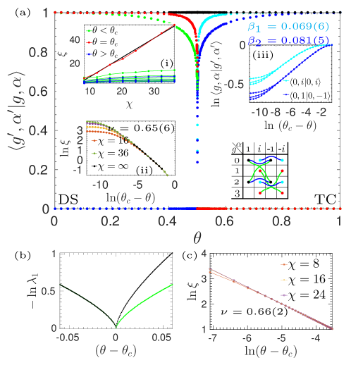
The order parameters in Fig. 6a and b show a different behavior around the phase transition: In Fig. 6a, they abruptly drop to zero, indicative of a first-order phase transition, while in Fig. 6b, they vanish continuously, corresponding to a second-order transition. This is confirmed by a careful analysis of the data around the phase transition: The insets (i) in the two panels show a magnified view of one of the order parameters (cf. label) in the vicinity of the phase transition for different values of : Clearly, both curves are well converged in , but show a fundamentally different behavior – discontinuous vs. continuous. This is also confirmed by plotting the order parameter vs. for different values of the interpolation parameter around the critical point, shown in the insets (ii): While for the 1st order transition, there is an abrupt change with a clear gap in the value of the order parameter at the phase transition, for the 2nd order transition its value changes smoothly, subject to a stronger -dependence around the transition. For the value of the phase transition, we find for the DS–TC interpolation, Fig. 6a, and for the QD–TC interpolation, Fig. 6b.
In the case of a second-order phase transition, we can additionally compute critical exponents , , for the various order parameters on both sides of the phase transition. For the QD–TC interpolation under consideration, we find for all non-trivial order parameters, consistent with an 2D Ising universality class, see inset (iii) in Fig. 6b.
V.2 Correlation length
The other relevant quantity which can be used to characterize the behavior at the phase transition is the scaling of correlation functions. In the case of topologically ordered systems, this can encompass both correlation functions of local observables as well as anyon-anyon correlation functions, which are described by string-order type correlators.
V.2.1 Computation
Within the framework of PEPS, there are several different ways to extract correlation lengths. We will now outline three different methods which we will make use of.
The first two are based on the fact that all correlations within PEPS are mediated by the transfer operator (Fig. 1e). Specifically, both the decay of arbitrary two-point correlations and of anyon-anyon correlation functions are determined by the leading eigenvalues of the transfer operator. In order to obtain the spectrum of the transfer operator, we can follow two routes: (1) We can use exact diagonalization of the transfer operator on an infinitely long cylinder with finite perimeter to obtain the correlation length and then extrapolate in (using a fit ) to get a reliable estimate of in the thermodynamic limit. In order to get access to both local and anyon-anyon correlations, the exact diagonalization has to be performed on all sectors of the transfer matrix, i.e., including the possibility of inserting a flux () in the ket (bra) layer when closing the boundary, and labeling the eigenvectors by their topological charge (i.e., irrep label) and ; the sector of the corresponding correlation function is then given by the difference of ket and bra flux and charge schuch2013topological . The overall correlation length can be computed from the gap in the spectrum of the transfer operator below the largest ground space sector – in the case of -invariant tensors with ground states, . (2) Alternatively, we can compute the gap of the transfer operator by determining its fixed point in the thermodynamic limit using an iMPS ansatz, and then using an iMPS excitation ansatz as proposed in pirvu2012matrix ; haegeman2012variational ; haegeman2013post to model the excitations. In particular, the excitation ansatz allows to also explicitly construct topologically non-trivial excitations by attaching a flux string (=symmetry action) to the excitation and giving it a non-trivial charge (=irrep label), and thus allows to access the different topological sectors haegeman2015shadows .
Finally, a third method to extract a correlation length is to use the channel operator corresponding to the fixed point of the transfer operator (Fig. 5f), whose spectrum can be computed efficiently as it is system size independent. The correlation length can again be extracted from the subleading eigenvalues of the channel operator, as well as the the leading eigenvalues of the dressed channel operator , and additionally using irrep labels of the eigenvectors to fully address anyonic correlations. Note, however, that this approach in principle only gives access to correlations along a specific axis.
V.2.2 Analysis
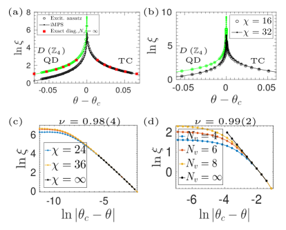
Let us now analyze the information obtained from the different methods. We start by a comparison of the methods for the 2nd order QD to TC transition in Fig. 7. Panel (a) compares the results obtained from the different methods, which are in very good agreement. (Data from finite cylinders is only shown in the regime where the extrapolation to works reliably.) Fig. 7b shows the correlation length extracted from the channel operator of the iMPS fixed point, labelled by its flux. We see that on the left of the phase transition, the dominating correlations are those between fluxful anyons, which indicates that the transition from the QD phase is driven by condensation of fluxes (or dyons), in accordance with what is observed in Fig. 6b where the fluxes are condensed in the TC phase. Fig. 7c,d finally show the extraction of the critical exponent from iMPS data, extrapolated in (panel c), and finite cylinder data, extrapolated in (panel d), which are in very good agreement.
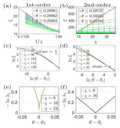
Fig. 8 compares the results for the 1st order transition from DS to TC (left column) with the 2nd order transition from QD to TC (right column). We find that in the 1st order case, the correlation length obtained from iMPS converges linearly in to a constant [Fig. 8a], while in the 2nd order case, it diverges approximately linearly in [Fig. 8b]; also note that in this case the correlation is already for a bond dimension . Fig. 8c,d shows the scaling of in the vicinity of the phase transition as it is approached from the left. While in the 1st order case, the curve leaves the initial scaling as the transition is approaching, and this behavior does not depend on , the scaling in the case of the 2nd order transitions approaches the scaling closer and closer to as is increased. Finally, Fig. 8e,f shows the inverse correlation length as extracted from the diagonalization of the transfer operator using an excitation ansatz: We find that the eigenvalue gap in the first-order case, while small, remains open, while it closes in the second-order case.
V.3 Further probes
Our main tools to analyze phase transitions will be correlation length and order parameters. However, there are a number of other probes which allow us to look more closely at phase transitions, and which we describe in the following.
V.3.1 Fidelity susceptibility
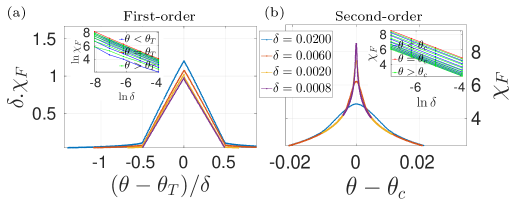
The overlap between ground state wavefunctions, known as fidelity, has been pointed out as a probe in order to study quantum phase transitions zanardi2006ground . More specifically, the fidelity susceptibility
| (39) |
where is the fidelity per site as a parameter changes from to , exhibits universal features which can be used to characterize phase transitions zanardi2007information . An account on the behavior of fidelity per site and its computation using iMPS algorithm is given in Appendix A.
In the following, we discuss the distinct features of for the two above mentioned phase transitions, showing clearly distinct signatures for 1st and 2nd order transitions. The data is shown in Fig. 9 for different values of the step size . In both cases, diverges at the phase transition. However, the divergence is very distinct: In the case of the 1st order transition between DS and TC, converges to a delta function as , as can be seen from the rescaled plot in Fig. 9a, which shows that for a universal triangle-shaped function . This is in accordance with the expected abrupt change of the ground state wavefunction (even per unit cell) at a first order phase transition. For the 2nd order transition between QD and TC, on the other hand, as . (Since we expect to scale like the structure factor for an observable relating to the derivative of the local PEPS tensor zanardi2007information ; schuch:rvb-kagome , which scales like the corresponding correlation length squared, we expect to only diverge logarithmically with , in agreement the fact that we are considering a topological phase transition.)
V.3.2 Susceptibility
Order parameters measure the amount of spontaneous symmetry breaking in the system. Further universal information about order parameters can be extracted by computing their susceptibility, this is, the scaling of their response to an infinitesimal field which explicitly breaks the symmetry in the vicinity of the phase transition,
| (40) |
The resulting critical exponent allows to further characterize the phase transition.
In the case of topological phase transitions, will be an order parameter for condensation or deconfinement. The external field corresponds to adding an infinitesimal term to the PEPS tensor which explicitly breaks the symmetry of the transfer operator in favor of one fixed point. An example, including more details on the computation of the susceptibility as well as numerical results, is given in Sec. VI.2.1 in the discussion of the QD to TC transition.
V.3.3 Dispersion relations
Above, we have described how to use an excitation ansatz to extract the correlation length of a PEPS wavefunction directly in the thermodynamic limit. Using the same method, we can also obtain -dependent correlation functions, which give us further information about features of the dispersion relation of the system zauner2015transfer , and in particular about the mechanism driving the topological phase transition haegeman2015shadows . We present dispersion data for the DS to TC transition in Appendix B.
VI Numerics: Results
In the previous section, we have discussed various numerical probes for the study of topological phase diagrams. In the following, we will apply these techniques to systematically explore the whole phase diagram of -invariant tensor network states.
The main focus of this section will be the three-parameter family introduced in Sec. IV.1 which includes QD, TC, DS, and trivial phases. We start in Sec. VI.1 with summarizing the phase-diagram of the model, and discuss the different transitions of the model in Sec. VI.2 (transitions from the QD phase), Sec. VI.3 (transitions between TC and DS), and Sec. VI.4 (a phase transition with continuously varying exponents between DS and trivial phase). Finally, in Sec. VI.5 we discuss the families interpolating between TC/DS and trivial phases introduced in Sec. IV.2.
VI.1 Phase diagram of -invariant tensor network states
Our main object of interest will be the family of states defined in Sec. IV.1, and in particular Eq. (33), which by deforming a -invariant tensor allowed us to interpolate between the QD, Toric Code, Double Semion, and trivial phases.
The family in Eq. (33) is parametrized by three parameters . Fig. 10 shows a section through the phase diagram along the three hyperplanes on which any one of the three . The family includes the phase (green), two toric code phases – a TC (black) and a TC (blue), a DS model with symmetry (yellow), and a trivial phase (red). The color is based on RGB values given by the order parameters (red), (green), and (blue), which allow to distinguish all those phases, cf. Appendix C.
Before we discuss the individual phase transitions in detail, let us give an overview of our findings:
The majority of the transitions in the phase diagram are governed by the breaking of a single symmetry in the transfer operator, corresponding to the arrows in Fig. 4. Moreover, except for the DS model the fixed points on both sides of the transition do not exhibit non-trivial SPT order. Specifically, this encomasses the QD (with symmetry ) to TC transition (for both and TC), as well as the transitions from both TC models to the trivial phases. For all of these transitions, we find that they fall in the 2D Ising universality class, in accordance with the fact that they are described by a one-dimensional transfer operator undergoing a symmetry breaking transition. This includes in particular the transitions marked (I), (II), and (V) in Fig. 10. This behavior is robust also when considering direct interpolations of the transfer operator, rather than the interpolation shown in Fig. 10.
The transitions involving the DS model, on the other side, are more rich. On the one hand, there are transitions which are again described by the breaking of a single symmetry, namely the QD () to DS () transition, as well as the DS to trivial transition. Different from the previous case, however, the fixed point at the DS side of the phase transition exhibits non-trivial SPT order. This is reflected in the universality class of the transitions: While the QD to DS transition along line (III) is still Ising-type, the transition from the DS () to the trivial phase (not part of Fig. 10) seems to belong to the 4-state Potts universality class. Finally, the DS to trivial phase transition in Fig. 10 exhibits continuously varying critical exponents when moving between the lines (V) and (VI) along the plane, whose behavior does not seem to match known universality classes.
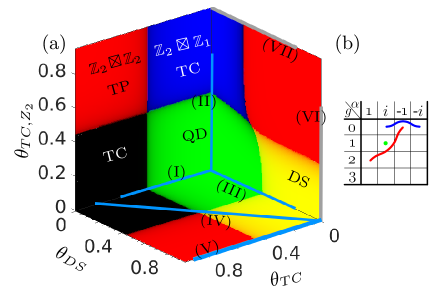
Finally, there are transitions between the DS model and TC models. There are two different types: First, the DS to TC transition, which corresponds to the breaking of two symmetries. While Fig. 10 does not exhibit such a transition, it is possible to obtain it by linear interpolation of the transfer operator. The transition is second order and lies in the universality class of the 4-state Potts model, in accordance with the breaking of a symmetry. On the other hand, there is the transition between the DS and the TC, which does not involve any symmetry breaking, but rather a re-ordering of the fixed point from a trivial to an SPT phase. As we have seen, this transition, when realized by direct interpolation, is 1st order; however, one can also realize a fine-tuned 2nd order transition through the quadro-critical point in the bottom plane of Fig. 10, line (IV), in which case a 2D Ising transition is observed.
Let us now discuss of findings for the individual transitions in detail.
VI.2 Transitions between QD and topological phases
VI.2.1 Transition between QD and TC
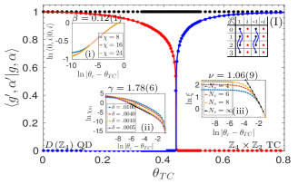
A transition between QD and TC can be obtained either by local filtering or by direct interpolation of the transfer operator, as described in Eq. (30) and Eq. (38), respectively. We have already considered the transition obtained by direct interpolation when introducing our methods in Sec. V, where we found a second-order transition in the 2D Ising universality class, Fig. 6b. In the following, we discuss the phase transition obtained by local filtering along the path labeled by (I) in Fig. 10a.
An important feature of this interpolation is that we can devise a microscopic mapping to the 2D Ising model, including an explicit mapping of condensate and deconfiment fractions to order parameters and twisted boundary conditions in the Ising model, see Appendix D; it thus allows us to benchmark our numerical methods with respect to the analytical results.
Fig. 11 gives the condensate fractions as indicated in the legend on the top right, identical to those in Fig. 6b, as a function of the interpolation variable . At the phase transition, the anyons become confined (red), while condenses (blue). The behavior of the order parameters clearly indicates a second-order phase transition. The numerical data (dots) and analytical data (lines) show excellent agreement, and the critical point is in agreement with the analytical value .
From the order parameters, we can extract the critical exponent , consistent with the analytical value , Fig. 11(i). A further critical exponent can be obtained by studying the suceptibility of the order parameter to an external “field”, cf. Sec. V.3.2: Here, the order parameter measures the spontaneous breaking of the symmetry. It can be explicitly broken by modifying the filtering tensor (30) as
| (41) |
where . The susceptibility is then defined as
| (42) |
where is a function of and . We have examined the behavior of by using finite differences for the derivative for different step sizes . The scaling of with respect to close to the critical point, Fig. 11(ii), gives a critical exponent , consistent with the analytical value . Finally, we have also determined the correlation length on an infinite cylinder, yielding a critical exponent , Fig. 11(iii), in agreement with the analytical value .
VI.2.2 Transition between QD and TC
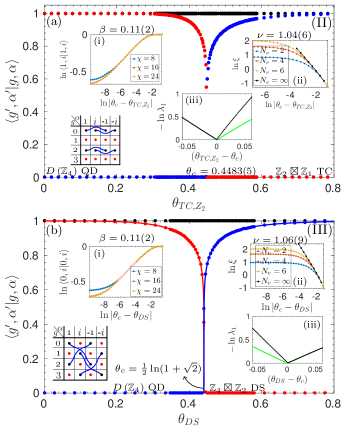
Let us now consider the phase transition between QD and TC labeled (II) in Fig. 10a; the TC is obtained from QD by condensing the charge rather than the flux as for the TC, leading to the confinement of the fluxes .
Fig. 12a summarizes the numerical results on the interpolation. The main panel shows the condensation and deconfinement fractions, as indicated in the bottom left. The data is consistent with a 2nd order phase transition at . The scaling of the order parameters yields a critical exponent [inset (i)], and for the correlation length, we find [inset (ii), from cylinders], both consistent with the 2D Ising universality class. Inset (iii) shows the inverse correlation length as extracted from the transfer operator using an excitation ansatz. Here, green dots correspond to topological excitations with a flux string attached (i.e., domain wall excitations of the broken symmetry ), and black dots to zero-flux excitations (both with and without charge); we thus find that the dominating length scale after the transition indeed arises from the confinement length of a flux (or dyon).
Let us add that we found that the phase transition between QD and TC constructed through direct interpolation of the transfer operator to lie in the Ising universality class as well.
VI.2.3 Transition between QD and DS
As a last transition out of the QD phase, we consider the transition to the DS model via the path (III) in Fig. 10a, Eq. (32). This transition can yet again be mapped to the 2D Ising model, cf. Appendix D. The results are shown in Fig. 12b, were in the main panel dots (lines) give the numerical (analytical) result: Numerical and analytical order parameters show excellent agreement, and we find a second order phase transition whose critical exponents match those of the 2D Ising model, with the transition at . In particular, inset (iii) shows again the subleading eigenvalue of the transfer operator, where green dots label sectors with a non-trival flux string; the dominant length scale before the transition thus arises from the mass gap of the dyon which is condensed in the DS phase.
VI.3 Phase transitions between toric codes and double semion model
Let us now turn towards phase transitions between the Toric Code and the Double Semion phase. This transition is of particlar interest, as it is not described by anyon condensation, and it has been conjectured that it should thus be first order, which is supported by exact diagonalization calculations morampudi2014numerical .
VI.3.1 Transition between TC and DS
Unlike for phase transitions which are described by condensation of anyons, obtaining an interpolation which achieves a direct transition between the TC and the DS phase is non-trivial and requires fine-tuning – for a generic interpolation, one would expect to go through an intermediate phase which has condensation-driven transitions to either TC and DS, i.e. either a trivial or a phase.
We had already earlier studied one direct transition between DS and TC in Sec. V, constructed by direct interpolation of the transfer operator, where we found that the transition was first order, cf. Fig. 6a and Fig. 8a,c,e.
Another possibility of obtaining a direct transition is to consider the horizontal plane () in the phase diagram Fig. 10, which exhibits a quadro-critical point in which TC, DS, trivial, and phases meet. As mentioned earlier, the whole plane can be mapped to the 2D Ising model, and so can a diagonal path [with ], labeled (IV) in Fig. 10a, which passes through the critical point at . The numerical findings along this interpolation are shown in Fig. 13a and are consistent with a phase transition in the 2D Ising universality class.
While the boundary states , of the TC and DS model both have symmetry, they differ in the projective action , of the generators and on the virtual indices of boundary MPS, cf. Eqs. (18) and (25): While in the case of the TC phase, the symmetry actions commute, in the DS phase they form a non-trivial projective representation equivalent to the Pauli matrices. This is in close analogy to the trivial vs. Haldane phase in the case of symmetry for 1D spin chains. These two phases can be distinguished by an order parameter which measures the commutator of the virtual symmetry actions. It can be computed from the iMPS description of by considering the normalized fixed points of its dressed channel operators (see Fig. 5b) as
| (43) |
given that the iMPS is in canonical form with (then, with unitary, cf. the discussion in Sec. V.1). Here, a value of () indicates that the system is in the TC (DS) phase haegeman2012order ; pollmann:spt-detection-1d . Fig. 13a(iii) shows in the vicinity of phase transition: It exhibits a sharp jump, which allows to accurately determine the value of the critical point.
VI.3.2 Transition between TC and DS
In contrast to the previous case, there does not exist a direct path between TC and DS in Fig. 10a on the hyperplane. We can however obtain a direct phase transition between the two phases by linear interpolation of the on-site transfer operators, cf. Eq. (38). The results are shown in Fig. 14: We find clear signs of a second order phase transition from DS to TC driven by simultaneous condensation of the anyon and de-condensation of the anyon, which is witnessed by a diverging correlation length and continuously vanishing order parameters.
The critical point is found at , which we can trace back to a self-duality of the model. Specifically, there exists a Matrix Product Unitary (MPU) which interchanges the on-site transfer operator of the DS and the TC fixed point when commuted with it; this implies that for the transfer operator of a column, . The explicit construction and analysis of the MPU is given in Appendix E. In fact, also interchanges the order parameters for the two phases, and thus, the order parameters in Fig. 14 are fully symmetric.
From the scaling of the correlation length at the critical point we extract a critical exponent . The order parameters exhibit two different critical exponents, which we determine as (for the deconfinement fraction ) and (for the condensate fraction ), respectively. Our findings for and are in accordance with the universality class of the Ashkin-Teller model at the -state Potts point (with and ), which is in agreement with the simultaneous breaking of two symmetries at the transition.
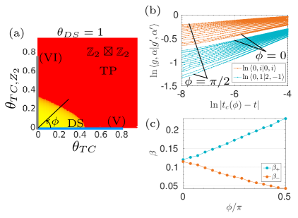
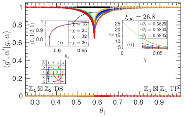
VI.4 Phase transition with continuously varying critical exponents
An interesting feature of the phase diagram of Fig. 10 is the transition between the DS and the trivial phase in the hyperplane spanned by the lines (V) and (VI) in Fig. 10. A cut through this hyperplane is shown in Fig. 15a. When moving along the plane, as parametrized by the angle , , we find that the transition is second order with critical exponent , but the critical expnents for the order parameters on the two sides of the transition change continuously. This is shown in Fig. 15b,c. Here, is the critical exponent of the order parameter in the DS phase, and is the critical exponent of the order parameter in the trivial phase. At , the transition is in the Ising universality class with . As we change , grows until the final value , while decreases until Let us add that the critical behavior is independent of the direction along which one crosses the phase transition, as to be expected.
Given the symmetries of the model, it is plausible to conjecture that this transition maps to the self-dual line of the Ashkin-Teller (AT) model which exhibits continuously varying critical exponents as well, including two different “electric” and “magnetic” exponents and baxter:book . However, there are several discrepancies, such as the constant as opposed to a continuously varying in the AT model, and the fact that in the AT model, and both change in the same direction, whereas and change in opposite directions, leaving the identification of the exact nature of this transition an open question.
VI.5 Phase diagrams of toric codes and double semion model
After having studied the phase diagram of the three-parameter family in detail, we will now proceed to examine the behavior of phase transitions which can have been constructed in Sec. IV.2 by further deforming the toric codes and double semion model down to trivial phases.
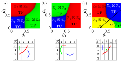
VI.5.1 Toric Code
In the case of toric code, the two-parameter deformation Eq. (IV.2.1) can induce phase transition to either the TP or TP. The phase diagram of the model is shown in Fig. 16a). Away from the tri-critical regime (where convergence becomes slow), we find that the phase transitions between the TC and either of the trivial phases lies in the Ising universality class.
VI.5.2 Toric Code
The two-parameter family of Eq. (IV.2.2) can drive the TC into the two trivial phases with and symmetry, respectively. The phase diagram is shown in Fig. 16b. At , the phase transition between TC and TP can be mapped to the 2D Ising model. Furthermore, away from the tri-critical regime, the transitions between TC and the two trivial phases are found to lie in the Ising universality class.
VI.5.3 Double semion model
Let us now turn to the two-parameter family of Eq. (36). It exhibits a DS phase, two trivial phases ( and ), as well as the QD phase. Fig. 16c shows the phase diagram. While the transitions between DS and QD across the horizontal axis and between DS and TP across the vertical axis lie in the Ising universality class, the transition from DS to the trivial phase is different: One the one hand, it requires fine-tuning to achieve a direct transition, which we obtain along the black line in Fig. 16c given by through the transition point , and on the other hand, it exhibits clear signs of a first order transition, as shown in Fig. 17.
VII Conclusions
In this paper, we have used the framework of PEPS to study topological phase transitions. Using the formalism of -injective PEPS, we have to set up families of models which interpolate between different topological phases, and have utilized the description of topological excitations in PEPS through string operators on the entanglement degrees of freedom to set up order parameters characterizing condensation and deconfinement of anyons, which allowed us to study the topological phases of these models and the transitions between them.
Starting from a model with symmetry, we have obtained a family of states encompassing the quantum double, toric code, double semion, and trivial phases, and set up interpolations between them. Using order parameters for condensation and deconfinement, anyonic correlation functions, and some further probes, we have characterized the phase diagram of the model. We found a rich structure where all possible phases and the transitions between them are realized. Analyzing the phase transitions revealed a range of different types of transitions, both first and second order. We found a number of transitions in the 2D Ising universality class, compatible with the understanding that these transition break a single symmetry, but also transitions in the 4-state Potts universality class, as well as transitions with continuously varying exponents whose universal behavior is not yet identified. We also found that the transition between double semion and toric code could be both first and second order, and exhibit different critical exponents.
It would be interesting to further investigate the nature of a generic interpolation between the toric code and the double semion model. If one would find that an interpolation between these phases (or any other two phases) is generically first order, this would also have implications on the results obtained with fully variational PEPS calculations, where the tensor could change abruptly at the phase transition: Having generically a first order transition implies that there is a range of values of the order parameters which cannot be reached by any choice of parameters, suggesting that the first order transition will persist even if considering a fully variational simulation.
The order parameters employed in this work for the analysis of topological phase transitions are not restricted to explicitly designed families of tensors: They can also be applied to scenarios where the tensors are obtained variationally by minimizing the energy of a given Hamiltonian, as long as the numerical method keeps track of the different topological symmetry sectors in the tensor. Note that this does not rule out explicit breaking of the symmetry which is important to obtain the best variational wavefunctions, as long as the sector label of the symmetry broken tensor is being kept track of as well. It would thus be interesting to use these order parameters for condensation and confinement to analyze the behavior of further topological phase transitions through variational PEPS calculations.
Acknowledgements.
MI thanks Manuel Rispler for helpful discussions. Part of the computations were performed on the JARA-HPC cluster at RWTH Aachen University, supported by JARA-HPC grant jara0092. This work was supported by the DFG through Graduiertenkolleg 1995, and the European Union through the ERC Starting Grant WASCOSYS (No. 636201).
Appendix A Phase transitions and fidelity per site
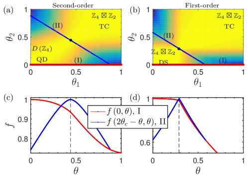
The notion of fidelity per site has been studied in the context of tensor network states in fid4 . It gives a measure of distinguishably between quantum states and it is defined as the normalized overlap of two wavefunctions per site.
| (44) |
and in the thermodynamic limit. Let
| (45) |
where
![[Uncaptioned image]](/html/1712.04021/assets/x74.png)
|
(46) |
is the on-site transfer operator and the top and bottom tensors in Eq. (45) are the local tensors for the left and right fixed point of the transfer operator computed using iMPS algorithm. Let be the largest eigenvalue of , then
| (47) |
Fidelity per site can used to characterize the behavior of phase transitions. Fig. 18 show a comparison of fidelity per site for (a) second- and (b) first-order phase transition. Fig. 18(c,d) shows the behavior of fidelity per site across different slices marked in the surface plot Fig. 18(a,b). Although, changes smoothly in the first-order case we observe a cusp like behavior in the transition regime which is qualitatively different in comparison to the second order phase transition between the QD and TC.
Appendix B Excitation spectrum of the transfer operator
We analyze the dispersion relation of the transfer operator. The computation of the low-lying excited states of the transfer operator has been achieved by using the excitation ansatz haegeman2013post . We present our findings for the phase transition between DS and TC phase, where the fixed points of the transfer operator spontaneously break the symmetry to .
Since the transfer operator is invariant, we can label each excitation of the transfer operator for the given as , where is a label for the conjugacy class and is a label for an irrep. of . It is important to note that the different species of anyonic particles in the TC and DS phase can be labeled by .
As the system is tuned from the DS phase towards the critical point, bosonic excitations get condensed to the vacuum, and this property is crucial in determining the behavior of the system. Remarkably as first suggested in haegeman2015shadows , that condensation of bosonic anyons is manifested in the excitation spectrum of the transfer operator. The low lying excitations labeled as in Fig. 19a are identified with the condensation of bosons. Furthermore, the excitations labeled as and represent the deconfinement of and anyons respectively.
Similarly, on the other side of the critical point in TC phase, the behavior of the system is characterized by the condensation of magnetic anyons (labeled as in Fig. 19b). Excitation labeled as and manifest the deconfinement of semions and their conjugates.
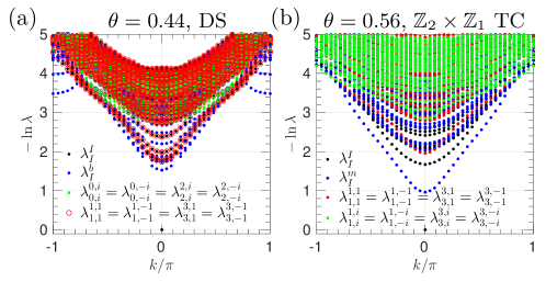
Appendix C RGB coding of the phase diagram
The phases in Fig. 10 are encoded using an RGB scheme, where the values for red, green, and blue are determined by the three fractions , , whose values are sufficient to visualize every phase which can be realized by deformation. In the following, we will explain the appearance of different phases in Fig. 10.
-
1.
In QD, none of the possible anyons are condensed or confined, which means that the only fraction from with a non-zero value is . So the green region in the phase diagram is identified with QD.
-
2.
In the case of TC, all the anyons of form are confined, which implies that the overlaps and are equal to zero. Furthermore, the anyon is condensed to the vacuum but it can be distinguished from the anyon . Since every fraction in is zero for TC phase, every point in the black region corresponds to TC.
-
3.
In TC phase, anyons of the form and are confined. Anyons and are not confined but they can be distinguished from each other. The only fraction in with a non-zero value is which explains the blue color for TC.
-
4.
Anyons are confined in DS phase which implies that the overlap is zero. On the other hand, the anyon is deconfined and the anyons and are mutually indistinguishable (i.e. ). The fractions in with non-zero value are (green) and (red). Sum of red and green produces yellow, so the DS phase is identified with yellow region.
-
5.
In the case of TP the only non-zero fraction from with a non-zero value is which determines the color of TP phase to be red.
Appendix D Ising model and topological phase transitions
In this appendix, we discuss a mapping between the partition function of classical Ising model and the norm of vacuum state which is parametrized by the tuning variable . We will focus our attention here to the phase transition between QD and TC, but the description is generic enough to be applied in other cases.
D.1 Classical Ising model
We begin by writing down the partition function in terms of Ising variables assigned to each vertex (Fig. 20a).
| (48) |
For later purposes, it will be convenient to interchangeably use binary variables and , where , to express each Ising configuration. We use the following graphical notation to represent Boltzmann weights on the horizontal and vertical edges of square lattice.
| (49) |
It is possible to construct a defective edge by inserting a Pauli- between connecting sites, which modify the Boltzmann weights as follows
| (50) |
We use here a blue line to indicate the presence of Pauli- (or ) at an edge in Eq. (50). Its presence at an edge switches the interaction from ferromagnetic to anti-ferromagnetic while preserving the whole object as a valid partition function. Pauli- at an edge also denotes the symmetry action. It is possible to have a tensor network description of the partition function where all the local tensors are invariant under the action of on all the legs. It also implies that a partition function with a string of ’s will remain invariant under any continuous deformation in the string provided that the endpoints remain fixed.
At this point, it is instructive to write down an analytic expression for expectation value of average magnetization per two sites.
| (51) | ||||
where the horizontal and vertical links in the product are expressed by an inclined edge. The cross sign on the edge indicates local order parameter on the vertices labeled 0 and 1. Although, the link has negative weights, in analogy to Eq. (50), we define it as follows.
| (52) |
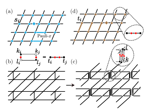
D.2 Anyonic vacuum and excitations
An important object to inspect in order to analyze the norm of a quantum state is the on-site transfer operator. We start by writing it pictorially for QD with deformation.
| (53) |
where each black circle in the sum with label denotes and is the generator of with regular representation. The outline of circles specifies Hermitian conjugate. Red bubbles represent deformation . The last equality is possible since black and red circles commute and the on-site tensors are isometric. The deformation modeled by red bubble drive the system from QD to TC phase. Using Eq. (53) we can write the norm of vacuum as
| (54) |
where the product is over all the rings (Fig. 20(b,c)) and by using Eq. (53) we can shrink each ring
![]() to an edge
to an edge
![]() with the following definition.
with the following definition.
| (55) | ||||
Each edge can be identified as an interaction in Ising model on square lattice. In order to be succinct we will write
![]() as
as
![]() . Since the Boltzmann weighs are zero if (mod 2), we can write Eq. (54) as a sum over two copies of Ising model on square lattice (Fig. 20b).
. Since the Boltzmann weighs are zero if (mod 2), we can write Eq. (54) as a sum over two copies of Ising model on square lattice (Fig. 20b).
| (56) |
Terms in Eq. (48) behave analogous to Eq. (56). By identifying different combinations in Eq. (49) and Eq. (55) with each other we can write
which implies .
Now, consider the anyon excitation which gets confined as the system approaches the critical point. More precisely, the norm of is zero in the TC phase. Norm of the excitation, , contains the ring
![]() which shrinks to the edge
which shrinks to the edge
![]() . We can write the norm as
. We can write the norm as
| (57) | ||||
The brown diamond indicates a charge which is given by in the ket and bra layer. Trace over each configuration on the edge is defined as follows
| (58) | ||||
We summarize the Boltzmann weight of all the configurations for two models in Tab.1.
|
|
|
|
|
|
|
||
|---|---|---|---|---|---|---|---|
| mod 4 | |||||||
| mod 4 | |||||||
It is clear from the table that an edge
![]() corresponds to the evaluation of magnetization per site up to a weighting factor . Using Eq. (51) for magnetization per site and dividing by
corresponds to the evaluation of magnetization per site up to a weighting factor . Using Eq. (51) for magnetization per site and dividing by
in order to compensate for the weighing factor we get an analytic expression for the norm of .
| (59) |
Excitation gets condensed to the vacuum in TC phase. Rings
![]() create a string of defective edges. In order to be consistent with notation used in Eq. (50), we write
create a string of defective edges. In order to be consistent with notation used in Eq. (50), we write
![]() as
as
![]() . Tab.1 contains the Boltzmann weights for different configurations of
. Tab.1 contains the Boltzmann weights for different configurations of
![]() in column 6. Overlap of excitation with vacuum creates
a semi-infinite string of
in column 6. Overlap of excitation with vacuum creates
a semi-infinite string of
![]() edges (Fig. 20d).
In order to get an analytic expression for condensate fraction , we first map the model from 2D classical Ising on square lattice to 1D quantum Ising chain. Kramers-Wannier duality of 2D classical Ising manifest itself as 1D quantum Ising duality using disorder operators on dual lattice.
edges (Fig. 20d).
In order to get an analytic expression for condensate fraction , we first map the model from 2D classical Ising on square lattice to 1D quantum Ising chain. Kramers-Wannier duality of 2D classical Ising manifest itself as 1D quantum Ising duality using disorder operators on dual lattice.
| (60) |
and are Pauli matrices on (dual) square lattice. Using this transformation, a semi-infinite domain wall created by a string of ’s translates into point operator corresponding to magnetization per site on the dual lattice. Condensate fraction can be written analytically as
| (61) |
where is related to by .
We have computed analytically two condensate fractions in Eq. (59) and Eq. (61). The rest of non-zero but not constant overlaps can be proved equal to either of the two using following identities.
| (62) |
| (63) |
The equality holds for every value of along the phase transition. Analytic results conforms exactly with the numerical data in Fig. 11a.
The norm of vacuum for the phase transition between QD and TC with explicit symmetry breaking can also be mapped to classical Ising model where the Ising variables have different Boltzmann weights. QD DS phase transition also gives rise to an Ising model but the identification of Ising variables is subtle as the local tensor network description of DS model breaks the rotational symmetry.
D.3 Simplifications by explicit symmetry breaking
We conclude this appendix with a note on how explicit symmetry breaking can prove useful in simplifying the mapping between certain interpolations and classical models (not necessarily restricted to the Ising model). To this end, let us consider the interpolations between DS and TC and obtained by direct interpolation of the on-site transfer operators . In this case, it is straightforward to check that for all three on-site transfer operators, it holds that , where each acts on a ket-bra pair of indices, and projects onto the 4-dimensional space of ket-bra operators spanned by . This is, has a fully local block structure corresponding to the blocks , , which relates to the fact that all tensors in the family break the same symmetry (namely to ). By projecting locally onto, e.g., , we can break this symmetry explicitly, and thereby replace the corresponding interpolations with interpolations with a (ket+bra) bond dimension of . This, on the one hand, facilitates possible mappings to classical models (such as a mapping of the DS to TC interpolation to a loop model, and of the DS to interpolation to a classical transfer operator with breaking of a symmetry), and at the same time, it allows for more efficient numerical simulations, used e.g. for the large data in Fig. 8a.
Appendix E Unitary equivalence between DS and TC
In this appendix, we give an MPO construction of a unitary which transform the transfer operators of DS and TC into each other. It is helpful for later purposes to first write down the local tensors which represent the RG fixed points of two phases. In the case of DS model
| (64) |
Green ring is an MPO projector for DS applied on QD (black ring). In later usage, we will drop the subscripts in matrix notation. Similarly, for TC
| (65) |
Moreover, the on-site transfer operators (termed “double tensors” in the following) of two models have the same representation as given in Eq. (64) and Eq. (65). The transfer operator constructed by blocking the double tensors, , can be interpreted as a sum of alphabetic strings where each alphabet is either DS or TC double tensor. And the local tensor of the desired MPO unitary is expected to swap the double tensor of DS with the double tensor of TC. Local tensor should act to substitute the double tensor of DS with the double tensor of TC and vice-versa.
Motivated by the construction of discriminating string order parameters for topological phases in duivenvoorden2013symmetry , we start by writing the local tensor description of MPO .
| (66) |
where the top (bottom) index is identified with the row (column) index of the matrix and the arrow head points in the direction of column index. Now, we show why Eq. (66) is the right description of by showing its action on the on-site transfer operators. With defined in Eq. (66), its action on DS tensor is
| (67) |
where . Although, it is not very clear in above form, it is more insightful to understand the action by a unitary transformation. Consider a unitary with the following definition,
| (68) |
where the join of top(bottom) indices correspond to row(column) index of the matrix. By applying to Eq. (67), we obtain
| (69) |
where . Matrix entries across the main diagonal correspond to the four blocks (or fixed points since each block can be identified with a fixed point) of TC (see Eq. (20)). MPO projectors (blue and green rings) in Eq. (64) and Eq. (65) commutes with the black MPO of QD, so the action of on the DS tensor can be summarized as
| (70) |
where,
| (71) |
Now, we consider the action of on the local tensor of TC.
| (72) |
In order to study the structure of DS blocks, again we define a unitary
| (73) |
By doing a unitary transformation on Eq. (72),
| (74) |
The two blocks are completely identical and correspond to one of the symmetry broken fixed point of DS model. Similar to Eq. (70), the action of on tensor with the local tensor of QD produces the local tensor of DS model.
| (75) |
Furthermore, from the action of in Eq. (70) and Eq. (75), we can also verify that the following relation also holds between and the on-site transfer operators of DS and TC.
![[Uncaptioned image]](/html/1712.04021/assets/x145.png) |
(76) | |||
![[Uncaptioned image]](/html/1712.04021/assets/x149.png) |
where,
| (77) |
In order to obtain the equation of Sec. VI.3.2, we insert at one end of the transfer operator and by using Eq. (76) and by zipping to the other end of the transfer operator we can achieve the global action of as required.
References
- (1) X.-G. Wen, Quantum Field Theory of Many Body Systems (Oxford University Press, 2004).
- (2) F. Bais and J. Slingerland, Condensate-induced transitions between topologically ordered phases, Physical Review B 79, 045316 (2009), arXiv:0808.0627.
- (3) F. Verstraete and J. I. Cirac, Valence Bond Solids for Quantum Computation, Phys. Rev. A 70, 060302 (2004), quant-ph/0311130.
- (4) F. Verstraete and J. I. Cirac, Renormalization algorithms for quantum-many body systems in two and higher dimensions, arXiv preprint cond-mat/0407066 (2004).
- (5) R. Orus, A Practical Introduction to Tensor Networks: Matrix Product States and Projected Entangled Pair States, Ann. Phys. 349, 117 (2014), arXiv:1306.2164.
- (6) F. Verstraete, M. M. Wolf, D. Perez-Garcia, and J. I. Cirac, Criticality, the area law, and the computational power of PEPS, Phys. Rev. Lett. 96, 220601 (2006), quant-ph/0601075.
- (7) O. Buerschaper, M. Aguado, and G. Vidal, Explicit tensor network representation for the ground states of string-net models, Phys. Rev. B 79, 085119 (2009), arXiv:0809.2393.
- (8) Z.-C. Gu, M. Levin, B. Swingle, and X.-G. Wen, Tensor-product representations for string-net condensed states, Phys. Rev. B 79, 085118 (2009), arXiv:0809.2821.
- (9) N. Schuch, I. Cirac, and D. Pérez-García, PEPS as ground states: Degeneracy and topology, Ann. Phys. 325, 2153 (2010), arXiv:1001.3807.
- (10) O. Buerschaper, Twisted Injectivity in PEPS and the Classification of Quantum Phases, Ann. Phys. 351, 447 (2014), arXiv:1307.7763.
- (11) M. B. Şahinoğlu et al., Characterizing topological order with matrix product operators, (2014), arXiv:1409.2150.
- (12) N. Bultinck et al., Anyons and matrix product operator algebras, Annals of Physics 378, 183 (2017), arXiv:1511.08090.
- (13) J. Haegeman, V. Zauner, N. Schuch, and F. Verstraete, Shadows of anyons and the entanglement structure of topological phases, Nature communications 6 (2015).
- (14) K. Duivenvoorden, M. Iqbal, J. Haegeman, F. Verstraete, and N. Schuch, Entanglement phases as holographic duals of anyon condensates, Phys. Rev. B 95, 235119 (2017), arXiv:1702.08469.
- (15) A. Y. Kitaev, Fault-tolerant quantum computation by anyons, Annals of Physics 303, 2 (2003).
- (16) O. Buerschaper, M. Christandl, L. Kong, and M. Aguado, Electric–magnetic duality of lattice systems with topological order, Nuclear Physics B 876, 619 (2013).
- (17) M. Iqbal, D. Poilblanc, and N. Schuch, Semionic resonating valence-bond states, Physical Review B 90, 115129 (2014).
- (18) N. Schuch, D. Perez-Garcia, and I. Cirac, Classifying quantum phases using Matrix Product States and PEPS, Phys. Rev. B 84, 165139 (2011), arXiv:1010.3732.
- (19) J. Haegeman and F. Verstraete, Diagonalizing Transfer Matrices and Matrix Product Operators: A Medley of Exact and Computational Methods, Annual Review of Condensed Matter Physics 8, 355 (2017), arXiv:1611.08519.
- (20) M. Sanz, M. M. Wolf, D. Perez-Garcia, and J. I. Cirac, Matrix Product States: Symmetries and Two-Body Hamiltonians, Phys. Rev. A 79, 042308 (2009), arXiv:0901.2223.
- (21) This is the case for both a right- or a left-canonical gauge for , this is, the gauge where either the right or the left fixed point of the transfer operator of the iMPS representing alone is the identity.
- (22) N. Schuch, D. Poilblanc, J. I. Cirac, and D. Perez-Garcia, Topological order in the projected entangled-pair states formalism: Transfer operator and boundary hamiltonians, Physical review letters 111, 090501 (2013).
- (23) B. Pirvu, J. Haegeman, and F. Verstraete, Matrix product state based algorithm for determining dispersion relations of quantum spin chains with periodic boundary conditions, Physical Review B 85, 035130 (2012).
- (24) J. Haegeman et al., Variational matrix product ansatz for dispersion relations, Physical Review B 85, 100408 (2012).
- (25) J. Haegeman, T. J. Osborne, and F. Verstraete, Post-matrix product state methods: To tangent space and beyond, Physical Review B 88, 075133 (2013).
- (26) P. Zanardi and N. Paunković, Ground state overlap and quantum phase transitions, Physical Review E 74, 031123 (2006).
- (27) P. Zanardi, P. Giorda, and M. Cozzini, Information-theoretic differential geometry of quantum phase transitions, Physical review letters 99, 100603 (2007).
- (28) N. Schuch, D. Poilblanc, J. I. Cirac, and D. Pérez-García, Resonating valence bond states in the PEPS formalism, Phys. Rev. B 86, 115108 (2012), arXiv:1203.4816.
- (29) V. Zauner et al., Transfer matrices and excitations with matrix product states, New Journal of Physics 17, 053002 (2015).
- (30) S. C. Morampudi, C. Von Keyserlingk, and F. Pollmann, Numerical study of a transition between Z 2 topologically ordered phases, Physical Review B 90, 035117 (2014).
- (31) J. Haegeman, D. Pérez-García, I. Cirac, and N. Schuch, Order Parameter for Symmetry-Protected Phases in One Dimension, Physical Review Letters 109, 050402 (2012).
- (32) F. Pollmann and A. M. Turner, Detection of Symmetry Protected Topological Phases in 1D, Phys. Rev. B 86, 125441 (2012), arXiv:1204.0704.
- (33) R. Baxter, Exactly Solved Models in Statistical MechanicsDover books on physics (Dover Publications, 2007).
- (34) H.-Q. Zhou, R. Orús, and G. Vidal, Ground state fidelity from tensor network representations, Physical review letters 100, 080601 (2008).
- (35) K. Duivenvoorden and T. Quella, From symmetry-protected topological order to Landau order, Physical Review B 88, 125115 (2013).