Dynamic Freeze-In: Impact of Thermal Masses and Cosmological Phase Transitions on Dark Matter Production

Abstract

The cosmological abundance of dark matter can be significantly influenced by the temperature dependence of particle masses and vacuum expectation values. We illustrate this point in three simple freeze-in models. The first one, which we call kinematically induced freeze-in, is based on the observation that the effective mass of a scalar temporarily becomes very small as the scalar potential undergoes a second order phase transition. This opens dark matter production channels that are otherwise forbidden. The second model we consider, dubbed vev-induced freeze-in, is a fermionic Higgs portal scenario. Its scalar sector is augmented compared to the Standard Model by an additional scalar singlet, $S$, which couples to dark matter and temporarily acquires a vacuum expectation value (a two-step phase transition or “vev flip-flop”). While $\left\langle S\right\rangle\neq 0$, the modified coupling structure in the scalar sector implies that dark matter production is significantly enhanced compared to the $\left\langle S\right\rangle=0$ phases realised at very early times and again today. The third model, which we call mixing-induced freeze-in, is similar in spirit, but here it is the mixing of dark sector fermions, induced by non-zero $\left\langle S\right\rangle$, that temporarily boosts the dark matter production rate. For all three scenarios, we carefully dissect the evolution of the dark sector in the early Universe. We compute the DM relic abundance as a function of the model parameters, emphasising the importance of thermal corrections and the proper treatment of phase transitions in the calculation.

I Introduction

“In order for the light to shine so brightly, the darkness must be present.” This quote, attributed to Sir Francis Bacon, subsumes much of modern day cosmology. The Universe as we know it, with its abundance of bright galaxies, could not have formed without the presence of large amounts of dark matter (DM). DM drives the formation of structure; the gravitational collapse of primordial density fluctuations leads to dense objects like galaxy clusters, galaxies, and stars, with at least one of the latter harbouring life. Even though one of the lifeforms likes to describe itself as intelligent, it is still very much in the dark about dark matter, its origin and its nature.

For a long time, the best-motivated scenario to understand DM has been the Weakly Interacting Massive Particle (WIMP) scenario: DM particles are hypothesised to be heavy ($m_{\text{DM}}\gtrsim 100$ GeV) and to have weak, but non-negligible interactions with Standard Model (SM) particles. In the very early Universe, these interactions keep the DM and SM sectors in kinetic and chemical equilibrium, until eventually Hubble expansion dilutes the DM density to the extent that DM annihilation into SM particles ceases. This freeze-out typically occurs at temperatures $T$ where $x\equiv m_{\text{DM}}/T\simeq 25$ [1].

While freeze-out is arguably still the leading scenario for explaining the DM abundance in the Universe, the lack of experimental evidence for DM particles, in spite of a vigorous, multi-pronged search program [2, 3, 4, 5, 6, 7, 8], motivates the study of alternative mechanisms [9, 10, 11, 12, 13, 14, 15, 16, 17, 18, 19, 20]. Freeze-in models assume that the initial DM abundance after inflation was zero and that DM particles couple so weakly to the particles in the thermal bath that they never reach thermal equilibrium [17, 18, 19, 20, 21]. Consequently, DM annihilation does not determine the relic abundance. Instead, the observed abundance is the result of processes with DM in the final state, typically at $x\simeq 1$–$5$. The small coupling between DM and SM particles also implies a significantly greater challenge for all experimental probes of the nature of DM.

In this paper, we consider the impact of finite temperature effects on the DM abundance in freeze-in models. Such effects are manifold: first, particle masses receive corrections from thermal loops, implying that the kinematics of DM production is in general $T$-dependent. Certain production channels may be open during some epochs of cosmological history, but kinematically closed during others. Closely related to this effect is the $T$ dependence of the effective scalar potential $V^{\text{eff}}$, which implies that not only scalar masses (the second derivatives of $V^{\text{eff}}$), but also their vacuum expectation values (vevs) change with time in the early Universe. These vevs, in turn, will affect gauge boson and fermion masses (of course, gauge boson and fermion masses also receive direct corrections from self-energy diagrams evaluated at $T\neq 0$, although the contribution to fermion masses will be unimportant in the scenarios we discuss). The most interesting case is where the scalar potential develops several disjoint minima and transitions from one to another in a phase transition. The phase transition, for which the scalar vev is an order parameter, can be first order, second order, or a mere cross-over. The latter (and perhaps least interesting case) is realised in the SM [22, 23, 24, 25, 26].

In standard freeze-out scenarios, thermal effects are usually negligible since they are small at $x\gg 1$, i.e., at temperatures much lower than the masses of the involved particles. For freeze-in at $x\simeq 1$–$5$, on the other hand, they can be large and have a decisive impact on the DM abundance. Demonstrating this with several examples is the main topic of this paper.

To focus on the important effects and avoid unnecessary complications, we consider a toy model consisting of the standard model, a new gauge singlet scalar, and one or two gauge singlet dark sector fermions. Since we focus on freeze-in, we imagine some couplings to be $\ll 1$. As discussed below, these small couplings will often be technically natural (i.e., protected from large radiative corrections). In other cases, we assume a small coupling to simplify the analysis, but in these cases we do not expect a larger coupling to spoil the overall picture. The scenarios we consider could be motivated from a wide range of UV theories, including SUSY and extra dimensional scenarios [19]. Scenarios with gauge singlets at the weak scale are notoriously difficult to test at colliders and will not be ruled out at the LHC. The scenarios discussed in sections III and IV will be best probed through their $\mathcal{O}(1)$ Higgs portal couplings, but the full parameter space will not be probed until a 100 TeV collider has collected 3 ab^-1 of integrated luminosity [27]. The scenario discussed in section II is even harder to exclude, due to the small Higgs portal coupling.

The impact of thermal effects in the early Universe on the DM abundance has been previously discussed for instance in [28, 29], where it was argued that DM could be temporarily unstable in the early Universe, so that its abundance would be controlled by its decay rates and by the temperature of the phase transition that stabilises it. Similar thermal effects have also been considered in, e.g., [30, 31].

The outline of the paper is as follows. In section II we discuss a scenario, dubbed “kinematically induced freeze-in”, in which the kinematics of DM production is controlled by the $T$-dependent masses of a new scalar $S$ and a new dark sector fermion $\psi$. DM particles $\chi$ freeze in through their couplings to $S$ and $\psi$, but for most of cosmological history DM production via $\psi\to S\chi$ is kinematically forbidden. However, as $S$ transitions from a phase with $\left\langle S\right\rangle=0$ to a phase with $\left\langle S\right\rangle\neq 0$, its mass drops close to zero and DM production becomes kinematically allowed for a short period of time. We emphasise that, in a more economical version of this model, $S$ could be replaced by the SM Higgs itself. In section III we consider an alternative freeze-in model — a variant of the fermionic Higgs portal scenario — in which the DM production rate in the dominant channels is proportional to $\left\langle S\right\rangle$. We call this scenario “vev-induced freeze-in”. There is a large region of parameter space where its scalar potential undergoes a two-step phase transition (“vev flip-flop”), i.e., the Universe starts out in a $\left\langle S\right\rangle=0$ phase, followed by an epoch with $\left\langle S\right\rangle\neq 0$. The electroweak phase transition ends this epoch and reverts the Universe to $\left\langle S\right\rangle=0$ (but a non-zero vev for the SM Higgs). It is thus the two phase transitions that control the DM abundance today. In a third model, which will be the topic of section IV, $\left\langle S\right\rangle$ controls mixing between the DM particle and a second new fermion. This mixing, in turn, opens up production channels that are otherwise inaccessible, thus boosting freeze-in production. Hence we call this scenario “mixing induced freeze-in”. We summarise and conclude in section V.

II Kinematically Induced Freeze-In: Temperature-Dependent Masses and Thresholds

In thermal quantum field theory, particle masses can receive temperature-dependent corrections from self-energy diagrams and thus become functions of $T$ themselves. For instance, the SM Higgs mass is $m_{h}(T=0)=125\,\text{GeV}$ today, but was much larger in the very early Universe and close to zero around the time of the electroweak cross-over at $T_{\text{EW}}\simeq 165\,\text{GeV}$. In this section we discuss a scenario where the kinematics of the DM freeze-in rate are controlled by the mass of a new real scalar $S$.

II.1 Toy Model

We consider a simple toy model — a variant of the fermionic Higgs portal scenario — whose particle content is given in table 1. Besides the real scalar $S$ and the Dirac fermion $\chi$, which is the DM candidate, we introduce a second new Dirac fermion $\psi$. All new particles are SM singlets, and $\psi$ and $\chi$ are charged under a $\mathbb{Z}_{2}$ symmetry. We remark already here that one could imagine a variation of the model in which $S$ is replaced by the SM Higgs field itself. The relevant terms in the Lagrangian at dimension four are

$$\mathcal{L} \supset\frac{1}{2}(\partial_{\mu}S)(\partial^{\mu}S)+\bar{\psi}(i\not{\partial}-m_{\psi})\psi+\bar{\chi}(i\not{\partial}-m_{\chi})\chi$$

$$\qquad+\big{[}y_{\psi\chi}\,\bar{\psi}S\chi+h.c.\big{]}+y_{\chi}\,\bar{\chi}S\chi+y_{\psi}\,\bar{\psi}S\psi-V(H,S)$$ (1)

with

$$V(H,S) =-\mu_{H}^{2}H^{\dagger}H+\lambda_{H4}\,(H^{\dagger}H)^{2}-\frac{1}{2}\mu_{S}^{2}S^{2}+\frac{\lambda_{S4}}{4!}S^{4}$$

$$\qquad+\frac{\lambda_{S3}}{3!}\,\mu_{S}S^{3}+\lambda_{p3}\mu_{S}\,S(H^{\dagger}H)+\frac{\lambda_{p4}}{2}\,S^{2}(H^{\dagger}H)\,.$$ (2)

The first line of eq. 1 contains the standard kinetic terms and the fermion mass terms. In the second line of eq. 1, we identify the Yukawa couplings between $S$, $\chi$ and $\psi$. We assume $y_{\chi}$ and $y_{\psi\chi}$ to be tiny to avoid full thermalisation of $\chi$ and thus allow for DM production via freeze-in rather than freeze-out. The smallness of $y_{\chi}$ and $y_{\psi\chi}$ could be motivated, for instance, by extra-dimensional scenarios where $\chi$ could be localised far away from $\psi$ and $S$ along the fifth dimension. The coupling $y_{\psi}$ on the other hand, is assumed to be sizeable so that $\psi$ and $S$ remain in thermal equilibrium until $T\ll m_{\psi},\,m_{S}$. Alternatively, one can also introduce an extra particle – for instance a second new scalar $S^{\prime}$ with negligible couplings to the DM particle $\chi$, but appreciable couplings to $\psi$ and to the SM sector – to achieve the same goal. In fact, in the numerical results shown below we will assume this second possibility because it simplifies the dynamics of the temperature-dependent effective scalar potential and opens up larger regions of parameter space than the vanilla scenario from eq. 1.

The first line of the scalar potential $V(H,S)$ in eq. 2 contains the mass terms and quartic couplings for $S$ and $H$. We assume $\mu_{H}^{2}\,,\mu_{S}^{2}>0$, so that not only $H$, but also $S$, may obtain a vev at tree level. The second line of eq. 2 consists of a cubic coupling for $S$ proportional to $\lambda_{S3}$ and of the cubic ($\propto\lambda_{p3}$) and quartic ($\propto\lambda_{p4}$) Higgs portal couplings. We will assume that $\lambda_{S3}$, $\lambda_{p3}$, and $\lambda_{p4}$ are $\ll 1$. For $\lambda_{S3}$ this is just a simplifying assumption that could be relaxed at the expense of unnecessarily complicating our analysis. The smallness of $\lambda_{p3}$ and $\lambda_{p4}$ could again be motivated in extra-dimensional scenarios by localising $S$ and $H$ far from each other along the fifth dimension. We hypothesise, however, that $\lambda_{p4}$ is still large enough to keep $S$ in thermal contact with the SM particles at temperatures $T\simeq m_{S}$, when DM freeze-in happens. We find that these conditions are satisfied for $\lambda_{p4}\sim 10^{-3}$.

Field	Spin	$\mathbb{Z}_{2}$	mass scale
$S$	0	$+1$	$m_{S}(T=0)\simeq 5\,\text{GeV}$
$\chi$	$\frac{1}{2}$	$-1$	$m_{\chi}\simeq 50\,\text{GeV}$
$\psi$	$\frac{1}{2}$	$-1$	$m_{\psi}\simeq 50\,\text{GeV}$

Table 1: The new particles we introduce in section II with their respective charges and mass scales. All new particles are SM gauge singlets.

Where necessary, we will decompose $H$ into its components according to $H=\big{(}G^{+},(h+iG^{0}\big{)}/\sqrt{2})$, where $h$ is the neutral CP even SM-like Higgs boson and $G^{\pm}$, $G^{0}$ are the Goldstone modes. Moreover, we will often use the definitions $v_{S}\equiv\left\langle S\right\rangle$ and $v_{H}\equiv\left\langle h\right\rangle$ for the vacuum expectation values of $S$ and $h$.

Freeze-in of $\chi$ can proceed through the decays $\psi\to S\chi$ or $S\to\chi\bar{\psi}$, (depending on the relative magnitude of the $\chi$, $S$, and $\psi$ masses), and through the $2\to 2$ reactions $\psi S\to\chi S$ and $SS\to\chi\bar{\psi}$. The Feynman diagrams for these four processes are depicted in fig. 1. We will focus on masses such that $m_{\psi}+m_{\chi}>m_{S}(T=0)$ and $m_{\psi}-m_{\chi}<m_{S}(T=0)$. This implies that the decays $\psi\to S\chi$ and $S\to\chi\bar{\psi}$ are kinematically forbidden today. In the very early Universe, however, $m_{S}$ receives large thermal corrections $\propto T$, which can lift its value above $m_{\psi}+m_{\chi}$ and thus open up the channel $S\to\chi\bar{\psi}$. Later, around the time when $S$ develops a non-zero vev, $m_{S}(T)$ approaches zero and the channel $\psi\to S\chi$ becomes temporarily available. The decay rates and annihilation cross sections for the processes in fig. 1 are

$$\Gamma(\psi\to\chi S) =\frac{y_{\psi\chi}^{2}}{16\pi}\frac{(m_{\chi}+m_{\psi})^{2}-m_{S}^{2}(T)}{m_{\psi}^{3}}$$

$$\hskip 56.9055pt\times\sqrt{\big{[}m_{\psi}^{2}-(m_{\chi}+m_{S}(T))^{2}\big{]}\big{[}m_{\psi}^{2}-(m_{\chi}-m_{S}(T))^{2}\big{]}}\,,$$ (3)

$$\Gamma(S\to\chi\bar{\psi}) =\frac{y_{\psi\chi}^{2}}{8\pi}\frac{m_{S}^{2}(T)-(m_{\chi}+m_{\psi})^{2}}{m_{S}^{3}(T)}$$

$$\hskip 56.9055pt\times\sqrt{\big{[}m_{S}^{2}(T)-(m_{\chi}+m_{\psi})^{2}\big{]}\big{[}m_{S}^{2}(T)-(m_{\chi}-m_{\psi})^{2}\big{]}}\,,$$ (4)

$$\sigma(S\psi\to S\chi) \simeq\frac{y_{\psi}^{2}y_{\psi\chi}^{2}}{32\pi s^{2}(s-m_{\chi}^{2})^{3}}\Big{[}(s-m_{\chi}^{2})(5s^{3}+55m_{\chi}^{2}s^{2}+3m_{\chi}^{4}s+m_{\chi}^{6})$$

$$\hskip 142.26378pt-2s^{2}(s^{2}-18m_{\chi}^{2}s-15m_{\chi}^{4})\log\Big{(}\frac{m_{\chi}^{2}}{s}\Big{)}\Big{]}\,,$$ (5)

$$\sigma(SS\to\chi\bar{\psi})\big{|}_{v_{S}=0} \simeq\frac{y_{\psi}^{2}y_{\psi\chi}^{2}}{8\pi s^{3}}\bigg{[}2(s^{2}+16m_{\chi}^{2}s-32m_{\chi}^{4})\log\bigg{(}\frac{s+\sqrt{s(s-4m_{\chi}^{2})}}{s-\sqrt{s(s-4m_{\chi}^{2})}}\bigg{)}$$

$$\hskip 142.26378pt-4(s+8m_{\chi}^{2})\sqrt{s(s-4m_{\chi}^{2})}\bigg{]}\,.$$ (6)

In the last two expressions, we have taken the limit $m_{\psi}\simeq m_{\chi}$ and $m_{S}\simeq 0$. Moreover, we have set the width of $\psi$ to $\Gamma_{\psi}=0$. In eq. 6, we have also set $v_{S}=0$ because the full expression is fairly lengthy, and we will see below that the channel $SS\to\chi\bar{\psi}$ is very subdominant when $v_{S}\neq 0$. In our numerical analysis below, we of course use the full expressions.

Figure 1: Dark matter freeze-in reactions in the toy model of kinematically induced freeze-in, see eq. 1. For $S\psi\to S\chi$ and $SS\to\chi\bar{\psi}$, we do not show the diagrams with crossed $S$ lines.

It is important that, thanks to the non-zero $\left\langle S\right\rangle$ at low temperatures, $S$ can decay through its Higgs portal coupling $\lambda_{p4}$ (or also through $\lambda_{p3}$). If this decay was not present, $S$ would have a relic abundance that would be too large. For $m_{S}$ below the $W$ and $Z$ thresholds, the decay rate is

$$\Gamma(S\to f\bar{f}) =\sum_{f}\frac{y_{f}^{2}\,\theta_{hS}^{2}(T)\,m_{S}(T)}{8\pi}\bigg{(}1-\frac{4m_{f}^{2}}{m_{S}^{2}(T)}\bigg{)}^{3/2}\theta\big{(}m_{S}(T)-2m_{f}\big{)}\,.$$ (7)

Here, the sum runs over light fermions, $f=e,\,\mu,\,\tau,\,u,\,d,\,s,\,c,\,b$, and $y_{f}=\sqrt{2}m_{f}/v_{H}$ are the corresponding Yukawa couplings. The $h$–$S$ mixing angle is

$$\tan\theta_{hS}(T)=\frac{(\lambda_{p3}\mu_{S}+\lambda_{p4}v_{S}(T))v_{H}(T)}{m_{H}^{2}(T)-m_{S}^{2}(T)}\,.$$ (8)

In these expressions $v_{S}(T)$ and $v_{H}(T)$ are the $S$ and Higgs vevs, respectively. $S$ also couples to SM particles via annihilations. After the electroweak phase transition, the main annihilation process is $SS\to h^{*}\to f\bar{f}$, with cross section

$$\sigma v_{\text{rel}}(SS\to f\bar{f}) =\sum_{f}\frac{C_{f}y_{f}^{2}\lambda_{p4}^{2}v_{H}^{2}(T)}{32\pi(m_{H}^{2}(T)-4m_{S}^{2}(T))^{2}}\bigg{(}1-\frac{m_{f}^{2}}{m_{S}^{2}(T)}\bigg{)}^{3/2}\theta\big{(}m_{S}(T)-m_{f}\big{)}\,$$ (9)

in the non-relativistic limit. In this expression, $C_{f}$ is a colour factor. We will choose $\lambda_{p4}\simeq 10^{-3}$, which makes $S$ decays, inverse decays, and annihilations fast enough to keep $S$ in thermal equilibrium with the SM at all $T\lesssim m_{\chi}$, where DM freeze-in dominantly occurs. We have verified that this is always possible for $m_{\chi}>m_{S}\gtrsim 3$ GeV. If $S$ were not in thermal equilibrium during DM freeze-in, the model would not be invalidated, but the dark and visible sector temperatures would differ, complicating the analysis.

We will also assume that, while DM freezes in, $\psi$ remains in thermal equilibrium with the SM sector, either through $\psi\bar{\psi}\leftrightarrow SS$ or through interactions with a second new scalar $S^{\prime}$ as explained below eq. 2. The cross section for $\psi\bar{\psi}\to SS$ in the non-relativistic limit is

$$\sigma v_{\text{rel}}(\psi\bar{\psi}\to SS) =\frac{v_{\text{rel}}^{2}y_{\psi}^{4}}{24\pi}\frac{\sqrt{m_{\psi}^{2}-m_{S}^{2}(T)}\,\big{(}2m_{S}^{4}(T)m_{\psi}-8m_{S}^{2}m_{\psi}^{3}+9m_{\psi}^{5}\big{)}}{(m_{S}^{2}(T)-2m_{\psi}^{2})^{4}}\,,$$ (10)

where $v_{\text{rel}}$ is the relative velocity of the annihilating $\psi$ particles. Note the $v_{\text{rel}}^{2}$ suppression of the annihilation cross section. Eventually, $\psi$ will freeze out, and we ensure that this happens late enough for its relic abundance to make up a subdominant contribution to the DM density (less than $1\%$). Note that $\psi$ is not absolutely stable, but can decay even at $T=0$ through $\psi\to\chi(S^{*}/H^{*}\to f\bar{f})$. The rate of this decay is (for $m_{\psi}-m_{\chi}>m_{S}$, $(m_{\psi}-m_{\chi})/m_{\chi}\ll 1$, and $m_{f}=0$) given by

$$\Gamma(\psi\to\chi f\bar{f}) \simeq\sum_{f}\frac{C_{f}y_{f}^{2}y_{\psi\chi}^{2}\theta_{hS}^{2}(T)}{120\pi^{3}}\frac{m_{\psi}^{5}(m_{h}^{2}+m_{S}^{2})^{2}}{m_{h}^{4}m_{S}^{4}}\bigg{(}1-\frac{m_{\chi}}{m_{\psi}}\bigg{)}^{5}\,.$$ (11)

Here, the sum runs over all kinematically accessible SM fermion species. Since we treat fermions as massless, eq. 11 will not be accurate near any of the fermion mass thresholds. Even though $\psi$ freezes out with only a subdominant relic abundance, its decays may violate constraints if they happen around the time of recombination [32, 33, 34]. We therefore demand $\tau_{\psi}\equiv 1/\Gamma_{\psi}\gtrsim 10^{11}$ sec or $\tau_{\psi}\lesssim 10^{5}$ sec [33]. We have verified that for the parameter region we will discuss in the following, $\lambda_{p4}$ and thus $\theta_{hS}(T)$ can indeed be adjusted such that $\tau_{\psi}\gtrsim 10^{11}$ sec. Even in this case, care must be taken that the residual abundance of $\psi$ at the time of decay is tiny ($\lesssim 10^{-10}\times(\tau_{\psi}/10^{15}\,\text{sec})$ times the DM abundance) to avoid anomalous reionization [35]. We have checked that this can be automatically achieved for DM masses $\lesssim 1$ GeV. In this case, $\tau_{\psi}$ is large because the only decay channels available to $\psi$ are suppressed by the small Yukawa couplings of light quarks and leptons. At larger DM mass, the easiest way of ensuring compatibility of the model with reionization constraints is to introduce an auxiliary fermion $\chi^{\prime}$, with $m_{\chi}^{\prime}\ll m_{\chi}$, and with a Yukawa coupling to $S$ and $\psi$ chosen such that the decay $\psi\to\chi^{\prime}f\bar{f}$ is much slower than freeze-in of $\chi$, but still occurs significantly before recombination ($\tau_{\psi}\lesssim 10^{5}$ sec [33]).

II.2 The Effective Potential

To correctly describe the evolution of the scalar sector of the model from eqs. 1 and 2 in the hot early Universe, we must go beyond the tree level potential and consider the finite temperature effective potential $V^{\text{eff}}$ which includes radiative corrections and thermal effects. Since we assume the portal couplings $\lambda_{p3}$ and $\lambda_{p4}$ to be small, we can treat the evolution of the dark sector potential as independent from that of the visible sector potential (we will consider the case of large portal couplings in sections III and IV). We begin with the approximate tree level potential in the dark sector,

$$V^{\text{tree}}(S) \approx-\frac{\mu_{S}^{2}}{2}S^{2}+\frac{\lambda_{S4}}{4!}S^{4}\,.$$ (12)

The effective potential $V^{\text{eff}}$ is defined in the usual way [36]: one first rewrites the generating functional, $E[J]=i\log Z[J]$, as a functional of $v_{S}(x)$ instead of the external source field $J(x)$. (Here, $Z[J]$ is the partition function.) This is achieved by relating $J(x)$ with $v_{S}(x)$ via $v_{S}(x)=\delta E[J]/\delta J$. Note that, in the presence of an $x$-dependent external source, $v_{S}(x)$ becomes a function of $x$ as well. The effective action $\Gamma^{\text{eff}}$, which is in turn the spacetime integral of the effective potential $V^{\text{eff}}$, is given by a Legendre transform: $\Gamma^{\text{eff}}[v_{S}]=\int d^{4}x\,V^{\text{eff}}[v_{S}]\equiv-E[J]-\int d^{4}y\,J(y)\,v_{S}(y)$. We see that $\Gamma^{\text{eff}}$ has the property that $\delta\Gamma^{\text{eff}}[v_{S}]/\delta v_{S}=0$, that is, the vacuum configuration $v_{S}$, including all quantum corrections, is obtained from $\Gamma^{\text{eff}}$ using a variational principle. Of course, $\Gamma^{\text{eff}}$ itself needs to be computed perturbatively.

As we outline in more detail in appendix A, the leading corrections that distinguish $V^{\text{eff}}$ from $V^{\text{tree}}$ are the Coleman-Weinberg term $V^{\text{CW}}$ that corresponds to resummed 1-loop diagrams at $T=0$ [37], the thermal one-loop contribution [38], $V^{T}$, and the resummed series of higher order “daisy” diagrams, $V^{\text{daisy}}$ [39, 40, 41, 42]. With our assumption that $y_{\psi\chi}$, $\lambda_{p3}$, and $\lambda_{p4}$ are tiny, loops involving $H$ and $\chi$ are negligible. Loops involving $\psi$ could be relevant at temperatures not too far below $m_{\psi}$ if $y_{\psi}\gtrsim 0.01$. In the following we will assume $y_{\psi}\lesssim 0.01$ to simplify the analysis. As explained below eq. 2 this will require a different mechanism for keeping $\psi$ in thermal equilibrium throughout DM freeze-in. We have verified that our toy model can be phenomenologically successful also for larger $y_{\psi}$. For $y_{\psi}\lesssim 0.01$, the only relevant diagrams contributing to $V^{\text{eff}}$ are those involving the quartic coupling $\lambda_{S4}$. In other words, the sums in eqs. 29, 34 and 35 run only over $S$. The coefficient $n_{i}$, which can be interpreted as counting degrees of freedom (although see [42]), is $n_{S}=1$. As a function of the field value, the mass of $S$ is given by

$$m_{S}^{2} \simeq-\mu_{S}^{2}+\frac{\lambda_{S4}}{2}S^{2}\,.$$ (13)

$V^{\text{daisy}}$ also depends on the thermal, or Debye, mass, which is given by the 1-loop self energy at non-zero $T$. The Debye mass of $S$ is given by [39]

$$\Pi_{S}(T) =\frac{T^{2}}{24}(\lambda_{S4}+4y_{\psi}^{2})\,.$$ (14)

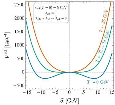
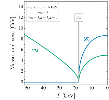
Figure 2: The new scalar effective potential at a relatively high temperature, at $T=T_{c}$ and at $T\sim 0\,\text{GeV}$, (left). A constant term has been subtracted at each $T$ so that $V^{\text{eff}}(0)=0$. The evolution of the new scalar mass and vev with temperature, (right), with the temperature of the phase transition indicated. Note that we neglect contributions from $\psi$ loops to $V^{\text{eff}}$, assuming $y_{\psi}\lesssim 0.01$.

With the effective potential in hand, we can now consider the evolution of $m_{S}$ and $v_{S}\equiv\left\langle S\right\rangle$ as a function of $T$. This allows us to describe the phase transition, which is analogous to the electroweak phase transition in the SM. We use the program CosmoTransitions [43, 44, 45, 46] to track the minimum of the effective potential, to find $\left\langle S\right\rangle$ as a function of $T$, and to determine the mass of $S$ as the second derivative of $V^{\text{eff}}(S)$. Although in our particular toy model it would be easy to do the computation without invoking CosmoTransitions, we still use it for consistency with sections III and IV.

The effective potential at several temperatures is shown in fig. 2 (left), while the behaviour of $\left\langle S\right\rangle$ and $m_{S}(T)$ is shown in fig. 2 (right). In the left panel we see the well known behaviour of a second order phase transition or cross-over: at high temperatures, $T\gg T_{c}$, the effective potential has its minimum at $S=0$. At the critical temperature, $T_{c}$, the minimum begins to move away from $S=0$ and a non-zero vev begins to develop. At the present time, near $T=0\,\text{GeV}$, the effective potential has its minimum at $S\simeq 9\,\text{GeV}$. In fig. 2 (right), we similarly see that at high temperatures, $S$ has no vev, and its effective mass is large thanks to thermal corrections $\propto T$. As the temperature drops, the mass of $S$ drops as well and approaches zero at the phase transition. This behaviour can be understood also from the green curve in fig. 2 (left): at the transition temperature, its second derivative at the minimum is zero. After the phase transition, the vev and the mass of $S$ grow and quickly approach their present day values, $m_{S}(T=0)=5\,\text{GeV}$ and $\left\langle S\right\rangle\simeq 9\,\text{GeV}$.

As well as this temperature dependence of the $S$ mass, the fermions may also have temperature dependent mass contributions. Since we take the tree level fermion masses to be much larger than the $S$ mass, self-energy diagrams evaluated at $T\neq 0$ will only give a small contribution near the phase transition (fermions have no zero Matsubara mode, so the self-energy contributions for fermions are smaller than those for bosons). However, if $y_{\psi}$ is large, then there can be significant corrections to the $\psi$ mass from the Lagrangian term $y_{\psi}\bar{\psi}S\psi$ when $S$ obtains its vev. The $T$ dependent $\psi$ mass is then

$$m_{\psi}(T)= \,m_{\psi}-y_{\psi}\left\langle S\right\rangle.$$ (15)

The crucial point for us is that, thanks to the behaviour of $m_{S}(T)$ and $m_{\psi}(T)$, the freeze-in channel $\psi\to\chi S$ is kinematically closed long before and long after the dark sector phase transition, while around the transition temperature, it is open and DM freeze-in can proceed efficiently.

II.3 Results and Discussion

In fig. 3 (top-left) we show the instantaneous DM yield from each freeze-in channel in fig. 1, including (solid lines) and ignoring (dashed lines) finite temperature contributions to the scalar masses and vevs and to the fermion masses. If we ignore the finite temperature corrections, only two channels ($S\psi\to\chi S$ and $SS\to\chi\psi$) contribute to the $\chi$ abundance. These contributions are largest at high temperatures (or small $x$, where $x=m_{\chi}/T$), where the abundance of $\psi$ is not Boltzmann suppressed and where $S$ have enough energy to produce the heavier states $\psi$ and $\chi$. The instantaneous freeze-in yield reduces smoothly as the temperature reduces, except for small steps where SM particles freeze-out and the effective number of relativistic degrees of freedom in the Universe, $g_{\text{eff}}$, changes.

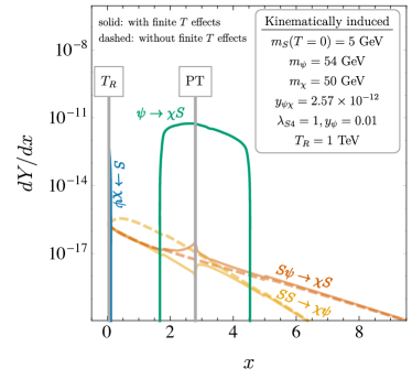
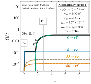
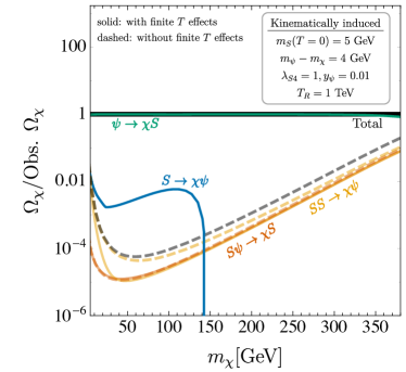
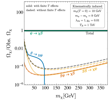
Figure 3: The instantaneous change in the yield (top-left) and the resulting freeze-in relic abundance extrapolated to the present day (top-right) for our benchmark point, including (solid lines) and ignoring (dashed lines) finite temperature effects. Also shown is the relative final abundance (normalised to the abundance when finite temperature effects are included) through each channel as a function of $m_{\chi}$ for $m_{S}(T=0)=5\,\text{GeV}$ (bottom-left) and $m_{S}(T=0)=10\,\text{GeV}$ (bottom-right).

If finite temperature effects are included, then two new channels contribute at different times. At very high temperatures, $S$ has a sufficiently large mass that it can decay to $\chi\bar{\psi}$. As $\chi$ and $\psi$ are much heavier than $S$ at $T=0\,\text{GeV}$, this channel is only open at very high temperatures ($x\lesssim 0.1$), and it no longer contributes at lower temperatures. As the Universe approaches the phase transition in the dark sector, the mass of $S$ reduces until it becomes smaller than $m_{\psi}(T)-m_{\chi}$ at $x\simeq 1.7$ (the mass of $\psi$ is constant before $S$ obtains its vev). At this point, the decay $\psi\to\chi S$ becomes kinematically possible and $\chi$ is produced. This happens at a rate much larger than that via the $S\psi\to\chi S$ and $SS\to\chi\psi$ channels because the latter channels are suppressed by the off-shellness of the intermediate $\psi$ propagator. The $\psi\to\chi S$ channel reaches its maximum rate around the dark phase-transition, where $m_{S}(T)$ goes to zero. As the temperature further reduces, the mass of $S$ increases and the mass of $\psi$ reduces until the channel closes at $x\simeq 4.5$. Comparing the rates with and without including finite temperature effects, we see that these effects are relevant in all channels. The rate of $S\psi\to\chi S$ shows a peak at the dark phase-transition because the intermediate $s$-channel $\psi$ propagator in the third diagram of fig. 1 can go nearly on-shell when $m_{S}(T)$ is small around the transition temperature. This is essentially a manifestation of the infrared divergence of the corresponding amplitude.

The resulting relic abundance of $\chi$ extrapolated to zero redshift is shown in fig. 3 (top-right). The extrapolated abundance at a given $x\equiv m_{\chi}/T$ is obtained by rescaling the number density at this time by the subsequent expansion of the Universe and normalising to the critical density today. Here we clearly see that the dominant contribution to the relic abundance comes from the $\psi\rightarrow\chi S$ channel. We emphasise that if finite temperature effects were not included, the calculated relic abundance would be incorrect by a factor $\mathcal{O}(10^{4})$. For the benchmark parameters chosen, the resulting $\chi$ abundance matches the observed relic abundance for $y_{\psi\chi}=2.57\times 10^{-12}$.

In fig. 3 (bottom-left) we show the abundance produced through each channel as a function of $m_{\chi}$, normalised to the abundance when finite temperature effects are included. We keep the mass difference between $\psi$ at $T=0$ and $\chi$ fixed at $4\,\text{GeV}$. The fraction of $\chi$ produced through channels other than $\psi\to\chi S$ is always small, but it is smallest for $m_{\chi}\simeq 50\,\text{GeV}$. At lower values of $m_{\chi}$, $S$ no longer requires significant thermal energy to produce $\chi$ via $S\psi\to\chi S$ and $SS\to\chi\psi$, so the $\psi\to\chi S$ channel produces a smaller fraction of $\chi$. As the value of $m_{\chi}$ increases, processes which occur at lower temperatures receive more Boltzmann suppression than those occurring at higher temperatures. This means that the amount of $\chi$ produced through $S\psi\to\chi S$ and $SS\to\chi\psi$ (which is important at high temperatures) is mildly reduced whereas the amount produced via $\psi\to\chi S$ (which is important around the phase transition) has greater Boltzmann suppression, reducing its relative importance.

Finally, fig. 3 (bottom-right) shows the freeze-in abundance of $\chi$ through the different channels for $m_{S}=10\,\text{GeV}$, where now the phase transition occurs at $T=36\,\text{GeV}$. We see that the picture is qualitatively similar to fig. 3 (bottom-left). For $m_{s}=10\,\text{GeV}$, there is a milder reduction in the relative importance of the $\psi\to\chi S$ channel at large $m_{\chi}$, due to a milder Boltzmann suppression of the $\psi$ abundance at the phase transition. In both fig. 3 (bottom-left) and (bottom-right), the yields due to $S\psi\to\chi S$ are similar including or ignoring finite temperature corrections. This channel predominantly produces $\chi$ at high temperatures, where the particle momentum dominates over the particle masses. For the small Yukawa coupling $y_{\psi}=0.01$ and large quartic coupling $\lambda_{S4}=1$, the $SS\to\chi\psi$ production rate is much larger when $S$ has a vev, which explains the difference seen between the curves that include or ignore the finite temperature corrections in this channel.

For definiteness in our numerical calculations, we fix a reheating temperature $T_{R}=1\,\text{TeV}$ which is sufficiently large so that any freeze-in at higher temperatures will produce negligible abundance of $\chi$.

We finish this section by noting a particularly simple model which shares many features with the toy model discussed above. If the SM is extended by two dark sector fermions, a SM gauge singlet, $\chi$, and an $su(2)_{L}$ doublet with hypercharge, $\psi$, then the SM Higgs can play the role of $S$ above. The Lagrangian term $\bar{\psi}H\chi+h.c.$ can lead to processes which produce $\chi$ via freeze-in. If $m_{\psi}-m_{\chi}<m_{h}(T=0)$ and $m_{\chi}<m_{\psi}$, then the channel $\psi\to\chi H$ will be open only when the mass of the SM Higgs is reduced during the second order electroweak phase transition. For $\psi$ lighter than 1.1 TeV, it freezes-out as a subdominant component of the dark matter abundance [47]. The remaining relic abundance can then be provided by the freeze-in of $\chi$. The calculation of the abundance is somewhat complicated and we defer this to later work.

III Vev-Induced Production with a Vev Flip-Flop

In the previous section we have highlighted the potential importance of including finite temperature corrections to particle masses in calculations of DM freeze-in. In this section, we consider a model with a fermionic DM candidate $\chi$ and with a scalar sector identical to the one in eq. 1, but focussing on a different region of parameter space. Namely, we now take the Higgs portal couplings so large that a two-step phase transition (or “vev flip-flop” [28]) is realised [48, 49, 50, 51, 52, 53, 27, 54] (see also [55]). In other words, the Universe goes through a phase where the new scalar $S$ obtains a non-zero vev, but this vev jumps back to zero in a first order electroweak phase transition. The value of $\left\langle S\right\rangle$ will control the DM freeze-in rate, so DM can only be efficiently produced during a relatively short time interval. The final DM abundance is determined not only by the relevant coupling constants, but also by the length of this time interval. We dub this mechanism “vev-induced production.”

III.1 Toy Model

The field content of the dark sector in this toy model is shown in table 2. As in section II, our dark matter candidate is a Dirac fermion, $\chi$, which is a SM gauge singlet. We assume that it is stabilised by a $\mathbb{Z}_{2}$ symmetry. The DM mass $m_{\chi}$ and the scalar mass parameter $|\mu_{S}|$ are taken to be $\simeq 100$ GeV. The relevant terms in the Lagrangian are

$$\mathcal{L} \supset y_{\chi}S\bar{\chi}\chi-V(H,S)\,,$$ (16)

with $V(H,S)$ again given by eq. 2. DM will freeze-in via the Yukawa coupling $y_{\chi}$; consequently, this coupling needs to be tiny. As in section III.1, this could be motivated in extra-dimensional scenarios by localising $\chi$ far away from the other fields along a fifth dimension. $\lambda_{S3}$ and $\lambda_{p3}$ are assumed to be small as well to simplify the analysis. Note that an extra global $\mathbb{Z}_{2}$ symmetry is restored if $y_{\chi}$, $\lambda_{S3}$, and $\lambda_{p3}$ are set to zero. Therefore, small values for these couplings are natural in the ’t Hooft sense [56]. Setting $\lambda_{p3}\ll 1$ means we can ignore mixing between the SM Higgs boson and $S$ at $T=0$. In this limit, the mass of $S$ is given by

$$m_{S}^{2}(T=0)=-\mu_{S}^{2}+\frac{\lambda_{p4}}{2}v_{H}^{2}(T=0)$$ (17)

at tree level and $T=0$. We see that for $\mu_{S}\simeq v_{H}(T=0)$ and $\lambda_{p4}\simeq 1$, a situation can be realised where $\lambda_{p4}v_{H}^{2}(T=0)/2>\mu_{S}^{2}$. In this case, $v_{S}(T)\equiv\left\langle S\right\rangle\neq 0$ as long as $v_{H}(T)=0$ (barring thermal corrections for the moment), but when $v_{H}(T)$ becomes significantly different from zero, the term quadratic in $S$ in the scalar potential experiences a sign flip, making $v_{S}(T)=0$ energetically favourable in the broken phase of electroweak symmetry. $v_{S}(T)=0$ is also realised at very early time thanks to thermal corrections to $V^{\text{eff}}$. These corrections are large especially when $\lambda_{S4}\gtrsim 1$. This behaviour is the gist of the vev flip-flop, and it defines the parameter region we will be interested in in the following: $\mu_{S}\simeq v_{H}(T=0)$, $\lambda_{p4}\simeq\lambda_{S4}\simeq 1$.

Field	Spin	$\mathbb{Z}_{2}$	mass scale
$S$	$0$	$+1$	$m_{S}(T=0)\simeq 100\leavevmode\nobreak\ \text{GeV}$
$\chi$	$\frac{1}{2}$	$-1$	$m_{\chi}\simeq 100\leavevmode\nobreak\ \text{GeV}$

Table 2: The dark sector of the vev-induced freeze-in scenario.

III.2 The Effective Potential & The Vev Flip-Flop

To quantitatively compute the effective potential for the model defined in eq. 16, the same methods as in section II.2 can be applied, but since the Higgs portal coupling $\lambda_{p4}$ is no longer negligible, we need to consider the joint evolution of the visible and dark scalar sector. In other words, we need to treat $V^{\text{eff}}$ as a function of both $S$ and $H$. As explained in sections II.2 and A, the one-loop contribution to the effective potential, $V^{\text{CW}}(h,S)+V^{T}(h,S)$, depends on the field dependent masses of all particles with couplings to the scalars. In the model from eq. 16, the field dependent masses of $W^{i},B$ and $t$ are the same as in the SM. In particular the gauge boson mass eigenvalues are $m_{W^{\pm}}^{2}=\tfrac{1}{4}g^{2}h^{2}$, $m_{Z}^{2}=\tfrac{1}{4}(g^{2}+g^{\prime 2})h^{2}$, $m_{\gamma}^{2}=0$, and $m_{t}=y_{t}h/\sqrt{2}$. Here, $g$ and $g^{\prime}$ are the $su(2)_{L}$ and $u(1)_{Y}$ gauge couplings, respectively, and $y_{t}$ is the top quark Yukawa coupling. The mass matrix of the neutral CP-even Higgs bosons is

$$m_{(h,S)}^{2}(h,S) =\begin{pmatrix}-\mu_{H}^{2}+\lambda_{p3}\,\mu_{S}S+\frac{1}{2}\lambda_{p4}\,S^{2}+3\lambda_{H4}\,h^{2}&(\lambda_{p3}\,\mu_{S}+\lambda_{p4}\,S)h\\ (\lambda_{p3}\,\mu_{S}+\lambda_{p4}\,S)h&-\mu_{S}^{2}+\lambda_{S3}\,\mu_{S}\,S+\frac{1}{2}\lambda_{S4}\,S^{2}+\frac{1}{2}\lambda_{p4}\,h^{2}\end{pmatrix},$$ (18)

while the mass of the neutral CP-odd and the charged component of $H$ are given by

$$m_{G^{+},G^{0}}^{2}(h,S) =-\mu_{H}^{2}+\lambda_{H4}\,h^{2}+\lambda_{p3}\,\mu_{S}\,S+\frac{1}{2}\lambda_{p4}\,S^{2}\,.$$ (19)

We can see that in regions where both $h$ and $S$ are non-zero, there will be mixing between the associated particles. Note that with our simplifying assumption $\lambda_{p3}\ll 0$, we can neglect $h$–$S$ mixing in the $\left\langle S\right\rangle=0$, $\left\langle h\right\rangle\neq 0$ phase at $T=0$. The sums in $V^{\text{CW}}(h,S)$ and $V^{T}(h,S)$ (see eqs. 29 and 34) now run over $i\in\{h,\,S,\,G^{0},\,G^{+},\,W^{i},\,B,\,t\}$. For $h$ and $S$, this is understood to mean summing over the neutral CP-even mass eigenstates, determined by diagonalising the mass matrix in eq. 18. The coefficients $n_{i}$ for the SM fields are $n_{h}=n_{s}=n_{G^{0}}=1$, $n_{G^{+}}=2$, $n_{W^{i}}=n_{B}=3$, and $n_{t}=-12$ [42]. The Debye masses of $h$ and $S$, relevant in the computation of $V^{\text{daisy}}$ (see eq. 35) are

$$\Pi_{h,G^{0},G^{+}} =\frac{T^{2}}{48}(24\lambda_{H4}+9g^{2}+3g^{\prime 2}+12y_{t}^{2}+2\lambda_{p4})\,,$$ (20)

$$\Pi_{S}(T) =\frac{T^{2}}{24}(\lambda_{S4}+4\lambda_{p4}+4y_{\chi}^{2})\,.$$ (21)

The Debye masses of $W^{i}$, $B$ and $t$ are the same as in the SM (see appendix A) as these particles do not couple to $S$. The sum in eq. 35 runs over $i\in\{h,G^{0},G^{+},S,W^{i},B\}$. The contribution of $\chi$ to the effective potential is negligible due to the smallness of $y_{\chi}$ and is therefore dropped in our calculations.

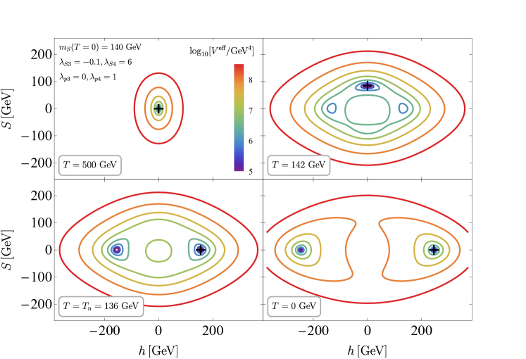
Figure 4: The effective potential $V^{\text{eff}}$ for a particular parameter point in the vev-induced DM production scenario defined in eq. 16. The black cross indicates the phase the Universe is in at the given temperatures. The two-step phase transition (“vev flip-flop”) is clearly visible: at $T=500\,\text{GeV}$ (top left), both $\left\langle S\right\rangle$ and $\left\langle h\right\rangle$ vanish, as $V^{\text{eff}}$ is dominated by thermal corrections. At a lower temperature, the Universe transitions to the $\left\langle S\right\rangle\neq 0$, $\left\langle h\right\rangle=0$ phase (top right), but eventually the minimum with $\left\langle S\right\rangle=0$, $\left\langle h\right\rangle\neq 0$ becomes the global one, so the Universe transitions into it and remains there (bottom left and bottom right).

The behaviour of the effective potential is illustrated in fig. 4 for a parameter point featuring a two-step phase transition or vev flip-flop. At early times (top left panel of fig. 4), $V^{\text{eff}}$ is dominated by the finite temperature and therefore approximately parabolic. Consequently, the SM Higgs and $S$ have zero vacuum expectation values. As the universe expands and cools down (top right panel of fig. 4), the finite temperature corrections become similar in magnitude to the tree-level terms and the effective potential develops minima at $\left\langle S\right\rangle\neq 0$. There is typically a second order phase transition, so the Universe immediately enters a phase where $S$ has a non-zero vev. After further cooling, new minima at $\left\langle h\right\rangle\neq 0$ develop. These become the global minima at some critical temperature $T_{c}$. However, there will now be a barrier between the $\left\langle S\right\rangle\neq 0$ and the $\left\langle h\right\rangle\neq 0$ minima, so the Universe cannot immediately transition into the global minimum, but undergoes a short period of supercooling. The subsequent phase transition is first order and proceeds via bubble nucleation, when at the nucleation temperature $T_{n}$ it becomes energetically favourable for bubbles of the new phase to expand and fill the entire universe. Typically, one finds $T_{n}\simeq T_{c}$, but in narrow regions of parameter space, $T_{n}$ may also be significantly below $T_{c}$. As in section II, we have used CosmoTransitions [43, 44, 45, 46] to determine the nucleation temperature. Numerically, CosmoTransitions computes $T_{n}$ by determining the temperature at which $S_{E}(T)/T$ drops below a critical value of 140. Here $S_{E}(T)$ is the minimum Euclidean action corresponding to a transition between the two potential minima [43]. The effective potential at $T=T_{n}$ is shown in the bottom left panel of fig. 4. The $h\neq 0$ minima then deepen as $T$ goes to zero, and the universe remains in a phase where $\left\langle S\right\rangle=0$ and $\left\langle h\right\rangle\neq 0$.

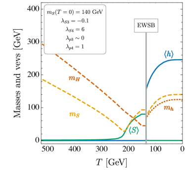
Figure 5: Evolution of the scalar vevs and masses with temperature for a particular parameter point in the vev-induced DM freeze-in scenario. $m_{H}$ denotes the mass of the SM Higgs doublet above electroweak symmetry breaking, while $m_{h}$ is the mass of the SM-like physical Higgs boson below.

In fig. 5 we show the masses and vevs of the new scalar $S$ and the SM Higgs doublet as a function of temperature. At high temperatures $\left\langle S\right\rangle$ is zero, but at lower temperatures it obtains a non-zero value. This situation persists until the first order electroweak phase transition at $T_{n}=136\,\text{GeV}$. At this point, $\left\langle S\right\rangle$ goes to zero while the SM Higgs vev becomes non-zero. $\left\langle h\right\rangle$ then gradually increases until it attains its $T=0$ value of $246\,\text{GeV}$. We can see that, as in fig. 4, the scalars receive large finite temperature corrections to their masses at high temperatures. For the parameters chosen here, both $m_{S}$ and $m_{h}$ become smaller than their $T=0$ values between the phase transitions, similar to what we found for $m_{S}$ in section III.2.

III.3 Dark Matter Freeze-In and Relic Abundance

In the model defined in eq. 16, the coupling $\lambda_{p4}$ between the new scalar field, $S$, and the SM Higgs doublet needs to be of order one for the vev flip-flop to occur (see discussion below eq. 17). Sizeable $\lambda_{p4}$ in turn means that at $T\simeq m_{S},\,m_{H}$, the scalar $S$ is in thermal equilibrium with the SM sector. $\chi$, on the other hand, never comes into thermal equilibrium because of our assumption that $y_{\chi}$ is tiny. Instead, a small abundance of $\chi$ is produced via freeze-in, facilitated by the processes $S\to\chi\bar{\chi}$, $H^{\dagger}H\to\chi\bar{\chi}$, and $SS\to\chi\bar{\chi}$. The corresponding Feynman diagrams are shown in fig. 6, and the decay rates and annihilation cross sections are

$$\Gamma(S\to\chi\bar{\chi}) =\frac{y_{\chi}^{2}}{8\pi m_{S}^{2}(T)}(m_{S}^{2}(T)-4m_{\chi}^{2})^{3/2}\,,$$ (22)

$$\sigma(SS\to\chi\bar{\chi}) =y_{\chi}^{2}(\lambda_{S3}\mu_{S}+\lambda_{S4}v_{S}(T))^{2}\frac{(s-4m_{\chi}^{2})^{3/2}}{8\pi s(m_{S}^{2}(T)-s)^{2}\sqrt{s-4m_{S}^{2}(T)}}\,,$$ (23)

$$\sigma(H^{\dagger}H\to\chi\bar{\chi}) =y_{\chi}^{2}(\lambda_{p3}\mu_{S}+\lambda_{p4}v_{S}(T))^{2}\frac{(s-4m_{\chi}^{2})^{3/2}}{8\pi s(m_{S}^{2}(T)-s)^{2}\sqrt{s-4m_{h}^{2}(T)}}\,.$$ (24)

The last expression should be understood as the cross section for one of the two components of the doublet $H$ to annihilate with its antiparticle into $\chi\bar{\chi}$. The first process, $S\to\chi\bar{\chi}$, is kinematically forbidden when $m_{S}(T)<2m_{\chi}$, but since thermal corrections may drive $m_{S}(T)$ to large values at $T\gg m_{S}(T=0)$, it may be allowed at early times. Whether or not this production channel is important will thus depend on the reheating temperature. We will be particularly interested in $T_{R}$ not too far above the electroweak scale, as in this case the dynamics of the vev flip-flop are most important for DM physics. The other two freeze-in processes can be mediated either by the cubic scalar couplings $\lambda_{S3}$, $\lambda_{p3}$, or by the quartic couplings $\lambda_{S4}$, $\lambda_{p4}$ if $v_{S}\neq 0$. We will focus on the parameter region where the cubic couplings are small because this is the region where freeze-in depends most strongly on $v_{S}$ and thus on the dynamics of the vev flip-flop. Moreover, as explained in section III.1, $\lambda_{S3},\,\lambda_{p3}\ll 1$ is technically natural in the ’t Hooft sense. We note, however, that $\lambda_{p3}$ should not be exactly zero. Otherwise, the small relic abundance of $S$ could not decay away and would violate direct detection limits. The small vev that $S$ has even at $T=0$ when $\lambda_{p3}\neq 0$ would not affect our results. It is also important to note that the restrictions we impose here on the parameters of the scalar potential and on $T_{R}$ are not necessary to make the model phenomenologically viable. There are other large regions of parameter space where the DM relic abundance can be successfully generated, albeit without strong involvement of the vev flip-flop.

Figure 6: The main production modes for the DM particle $\chi$ in the vev-induced freeze-in scenario.

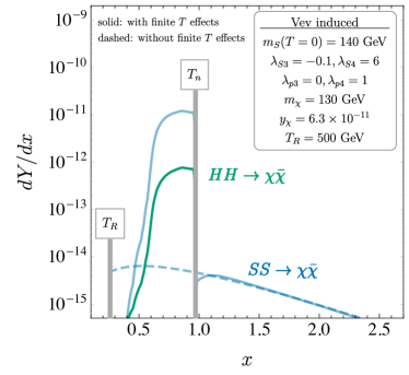
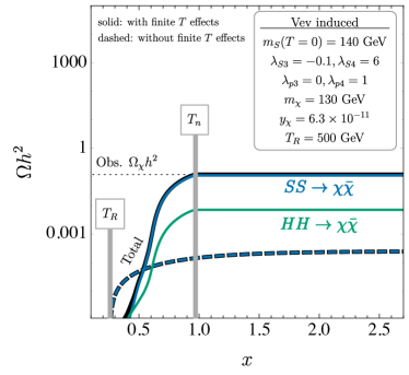
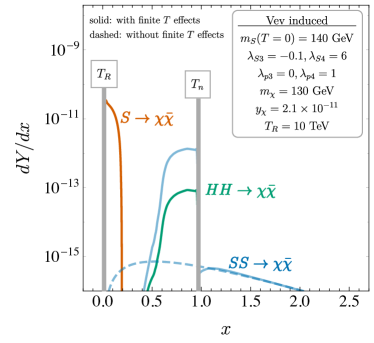
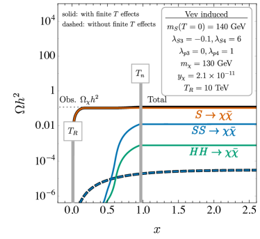
Figure 7: Evolution of the DM production rate (left) and the DM abundance extrapolated to $z=0$ (right) as a function of $x\equiv m_{\chi}/T$ for two different parameter points in the vev-induced freeze-in scenario defined by eq. 16. Solid curves correspond to the different production mechanisms shown in fig. 6. The dashed blue line indicates the result one would obtain if thermal corrections and the vev flip-flop were neglected. We see that for a reheating temperature $T_{R}$ just above the electroweak scale (top panels), the DM abundance is entirely dominated by the processes $H^{\dagger}H\to\chi\bar{\chi}$ and $SS\to\chi\bar{\chi}$, whose rates are greatly enhanced when $\left\langle S\right\rangle\neq 0$. For larger $T_{R}$ (bottom panels), the process $S\to\chi\bar{\chi}$, which is independent of $\left\langle S\right\rangle$, becomes allowed thanks to thermal corrections, even though at $T=0$, $m_{S}<2m_{\chi}$.

The DM production rate and the resulting abundance (extrapolated to zero redshift) are shown in fig. 7 for two illustrative parameter points of the vev-induced freeze-in scenario. The first parameter point shown in fig. 7 (top panels) is characterised by a low reheating temperature $T_{R}=500$ GeV. In this case, DM production is entirely dominated by $2\to 2$ processes proportional to $v_{S}$, so the dynamics of the vev flip-flop are crucial in this case. We see that the DM production rate $dY/dx$ rises rapidly after $S$ develops a vev at $T\simeq 250\,\text{GeV}$. Between the two phase transitions, $dY/dx$ follows the evolution of $v_{S}$, and the contribution from the $v_{S}$-dependent channels is 2–3 orders of magnitude larger than the contribution from vev-independent $SS\to\chi\bar{\chi}$ annihilation via $\lambda_{S3}$. Among the vev-dependent channels, $SS\to\chi\bar{\chi}$ dominates over $H^{\dagger}H\to\chi\bar{\chi}$ mainly because $\lambda_{S4}>\lambda_{p4}$. The small drop in $dY/dx$ immediately before the electroweak phase transition is due to the onset of Boltzmann suppression of $H$ and $S$. After the electroweak phase transition at $T\simeq 136\,\text{GeV}$, the $v_{S}$-dependent production processes cease. Before and after the two phase transitions, only the $v_{S}$-independent channel $SS\to\chi\bar{\chi}$ via $\lambda_{S3}$ is active, but its overall contribution is tiny. At $x\lesssim 0.5$, this channel is suppressed as the $s$-channel mediator, $S$, is very heavy at these high temperatures. Beyond the electroweak phase transition this channel gradually reduces, due to the Boltzmann suppression of $S$.

At the second parameter point shown in fig. 7 (bottom panels) the behaviour of the vev-dependent DM production channels and of vev-independent production via $SS\to\chi\bar{\chi}$ (mediated by $\lambda_{3}$) is similar to the top panels. However, as the second parameter point features a larger $T_{R}=10$ TeV, the decay channel $S\to\chi\bar{\chi}$, which does not depend on $v_{S}$ and on the vev flip-flop, is kinematically allowed at $x\lesssim 0.2$, when thermal corrections lift $m_{S}$ above $2m_{\chi}$. In this case, this production channel dominates the final abundance.

We conclude that, for low $T_{R}$, it is the dynamics of the vev flip-flop that determines the DM abundance today. For high $T_{R}$, it is the thermal corrections to $m_{S}(T)$, which in turn depend on the couplings in the scalar sector, especially $\lambda_{S4}$. In either case, the inclusion of thermal effects in the computation of the DM relic density is essential. To emphasise this point, we show in fig. 7 also the production rate and abundance that would be obtained if thermal corrections to $V^{\text{eff}}$ (and thus the two-step phase transition) were neglected in the calculation (dashed blue lines). In this case, only the processes $SS\to\chi\bar{\chi}$ and $H^{\dagger}H\to\chi\bar{\chi}$ with cross sections proportional to the small couplings $\lambda_{S3}^{2}$ and $\lambda_{p3}^{2}$, respectively, would contribute. For our choice $\lambda_{p3}=0$, only $SS\to\chi\bar{\chi}$ is open. The production rate in this channel is non-zero at $T_{R}$ (or even during preheating [57], which we neglect here assuming it is very rapid) and first rises slightly as there is more time to freeze-in at greater $x$. At $x\gtrsim 0.5$, the rate begins to drop as Boltzmann suppression becomes significant. Eventually, $\lambda_{S3}$-mediated production via $SS\to\chi\bar{\chi}$ freezes out.

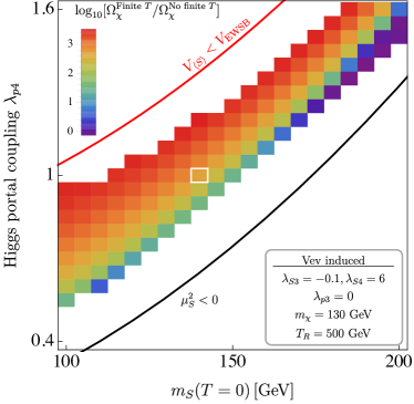
Figure 8: The ratio of the DM abundance including finite temperature effects to that ignoring finite temperature effects in the vev-induced freeze-in scenario. We show a cut through the parameter space of the model in the plane spanned by the zero temperature mass of $S$, $m_{S}(T=0)$, and the quartic Higgs portal coupling $\lambda_{p4}$. The white outline indicates the point considered in fig. 7.

We further explore the crucial importance of thermal corrections in fig. 8, which shows a cut through the model’s parameter space in the plane spanned by the zero temperature mass of $S$, $m_{S}(T=0)$, and the quartic Higgs portal coupling $\lambda_{p4}$. The pixelated region shows where the two-step phase transition occurs. The colour coding quantifies the ratio of the DM abundance obtained including thermal corrections to the abundance if these corrections were neglected for a low $T_{R}$. We see that thermal effects dominate the abundance by up to four orders of magnitude. For fixed $m_{\chi}$, they are largest at small $m_{S}(T=0)$, where thermal corrections to $m_{S}$ are most important, and at large $\lambda_{p4}$, where the $\left\langle S\right\rangle\neq 0$ phase lasts longer. For a high $T_{R}\sim 10\,\text{TeV}$, the freeze-in abundance is dominated by the $S\to\chi\bar{\chi}$ channel and thermal effects dominate the abundance by around four orders of magnitude over the whole parameter space shown. In the white area at the top of fig. 8, the global minimum of $V^{\text{eff}}$ at $T=0$ would be the one with $\left\langle S\right\rangle\neq 0$, i.e., electroweak symmetry would never be broken. In the white region at the bottom of the plot, $S$ never acquires a non-zero vev.

IV Vev-Induced Mixing with a Vev Flip-Flop

Let us now move to a third scenario illustrating the importance of thermal effects on the DM abundance in the Universe. The scenario discussed in the following, which we dub mixing induced freeze-in, is based on the same particle content as the kinematically induced freeze-in model from section II with an extra discrete symmetry. The model’s Lagrangian is thus given by eqs. 1 and 2, with the two forbidden Yukawa terms removed. The most important term for DM freeze-in is again the Yukawa coupling $y_{\psi\chi}\bar{\psi}S\chi$. However, we now assume the DM candidate $\chi$ and the new scalar $S$ to have masses around the electroweak scale, with $m_{S}>m_{\chi}$. The auxiliary new fermion $\psi$ is assumed to be much heavier (see table 3). The idea is that the reheating temperature is low, $T_{R}<m_{\psi}$, so that $\psi$ never comes into thermal equilibrium and DM production via $\psi\to S\chi$ (the channel we had focused on in section II) does not occur. Instead, the main DM production channels will be $S\to\chi\bar{\chi}$, facilitated by $\chi$–$\psi$ mixing through the $S\bar{\chi}\psi$ coupling, and $SS\to\chi\bar{\chi}$, mediated by a $t$-channel $\psi$ (see fig. 9). The former process is of particular interest to us because $\chi$–$\psi$ mixing depends on the vev of $S$. For the parameters of the scalar potential, we consider values similar to the ones we chose (and motivated) in section III: negligible $\lambda_{S3}$, $\lambda_{p3}$, but sizeable Higgs portal and dark sector quartic couplings, $\lambda_{p4},\,\lambda_{S4}\simeq\mathcal{O}(1)$, to induce a vev flip-flop. Thus, DM production via $S\to\chi\bar{\chi}$ will be open for a limited amount of time while $v_{S}\neq 0$. In the following, we will study the interplay of the two production processes, focusing in particular on the importance of $v_{S}$ and the vev flip-flop.

Field	Spin	$\mathbb{Z}_{2}$	$\mathbb{Z}_{2}^{\prime}$	mass scale
$S$	$0$	$+1$	$-1$	$m_{S}(T=0)\simeq 100\,\text{GeV}$
$\chi$	$\frac{1}{2}$	$-1$	$-1$	$m_{\chi}\simeq 100\,\text{GeV}$
$\psi$	$\frac{1}{2}$	$-1$	$+1$	$m_{\psi}>10^{3}\,\text{GeV}$

Table 3: The new particle content in the mixing induced scenario. All fields are SM singlets.

The decay width for $S\to\chi\bar{\chi}$ is

$$\Gamma(S\to\chi\bar{\chi}) =\frac{(y_{\psi\chi}\sin\theta_{\psi\chi})^{2}}{8\pi m_{S}^{2}(T)}(m_{S}^{2}(T)-4m_{\chi}^{2})^{3/2}\,,$$ (25)

and the cross section for $$SS\to\chi\bar{\chi}$$ reads

$$\sigma(SS\to\chi\bar{\chi}) \approx\frac{y_{\psi\chi}^{4}}{8\pi m_{\psi}^{2}}\frac{(s-4m_{\chi}^{2})^{3/2}}{s\sqrt{s-4m_{S}^{2}(T)}}\,,$$ (26)

where we have taken the limit $m_{\psi}\gg\sqrt{s},m_{S}(T),m_{\chi}$, which is justified in view of our assumption $m_{\psi}\gg T_{R}$. The mixing angle between $\chi$ and $\psi$ is

$$\theta_{\psi\chi}\simeq\frac{y_{\psi\chi}v_{S}(T)}{m_{\psi}}\,.$$ (27)

Figure 9: Feynman diagrams contributing to DM freeze-in in the mixing induced scenario. $\theta$ denotes the $\left\langle S\right\rangle$-dependent mixing angle between $\chi$ and $\psi$.

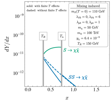
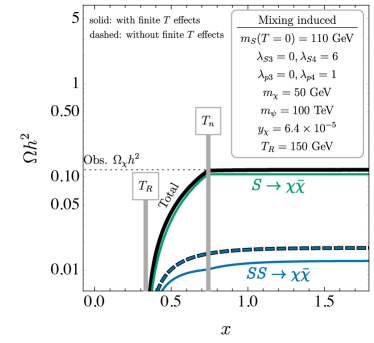
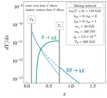
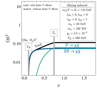
Figure 10: Evolution of the DM production rate (left) and the DM abundance extrapolated to $z=0$ (right) as a function of $x\equiv m_{\chi}/T$ for two different parameter points in the mixing induced scenario from section IV. Solid curves correspond to the different production mechanisms shown in fig. 9. The dashed curves indicates the result one would obtain if thermal corrections and the vev flip-flop were neglected. We see that for a reheating temperature $T_{R}$ just above the electroweak scale (top panels), the DM abundance is dominated by the mixing-induced decay $S\to\chi\bar{\chi}$, which is facilitated by the vev flip-flop. For larger $T_{R}$ (bottom panels), the process $SS\to\chi\bar{\chi}$, which is independent of $\left\langle S\right\rangle$, becomes relevant.

The dynamics of freeze-in via mixing are illustrated in fig. 10. In analogy to fig. 7 in section III, this figure shows the DM production rate and the extrapolated DM abundance as a function of $x\equiv m_{\chi}/T$. We again consider one parameter point with a low reheating temperature, $T_{R}=150$ GeV (top panels), and one parameter point with a higher reheating temperature, $T_{R}=500$ GeV (bottom panels). For low $T_{R}$, the DM abundance today is dominated by the decay $S\to\chi\bar{\chi}$, which is only possible for $v_{S}\neq 0$. For the parameters shown in the top panels of fig. 10, this phase is already realised at $T_{R}$. The rate for $S\to\chi\bar{\chi}$ increases along with $v_{S}(T)$ and then drops sharply to zero at $x\simeq 0.7$ as the electroweak phase transition switches $v_{S}$ off in favour of non-zero $v_{H}$. Similar behaviour is also seen for higher reheating temperature (bottom panels of fig. 10), but in this case, the overall importance of $S\to\chi\bar{\chi}$ does not dominate that of $SS\to\chi\bar{\chi}$. As the latter process is independent of $v_{S}$, it leads to DM production immediately after reheating (or already during preheating, which we neglect here), while $S\to\chi\bar{\chi}$ is only activated when $v_{S}$ becomes non-zero at $x\simeq 0.2$. Note from eq. 26 that for $T_{R}<m_{\psi}$ (the case realised in fig. 10), the DM production rate via $SS\to\chi\bar{\chi}$ scales $\propto T^{3}/m_{\psi}^{2}$. In other words, freeze-in is ultraviolet-dominated [58]. The dependence of $SS\to\chi\bar{\chi}$ on thermal corrections (namely the temperature dependence of $m_{S}(T)$) is relatively weak. It is reflected for instance in a jump in the rate at the electroweak phase transition. For comparison, we show also the production rate and DM yield in the absence of thermal corrections (dashed lines). We see that a calculation neglecting these corrections would fairly accurately predict freeze-in via $SS\to\chi\bar{\chi}$, but would completely miss the mixing-induced channel $S\to\chi\bar{\chi}$.

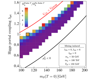
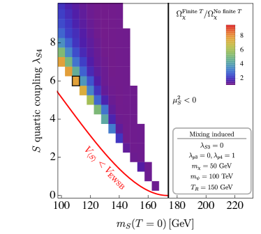
Figure 11: The ratio of the DM abundance including over ignoring finite temperature effects in the mixing induced scenario. We show a cut through the parameter space in the plane spanned by the zero temperature mass of $S$, $m_{S}(T=0)$, and the quartic Higgs portal coupling $\lambda_{p4}$ (left) and a slice of parameter space in the $m_{S}(T=0)$–$\lambda_{S4}$ plane (right). We see that the impact of thermal effects is largest at large portal coupling $\lambda_{p4}$ and small self-coupling $\lambda_{S4}$, where the $\left\langle S\right\rangle\neq 0$ phase lasts longer. The black outline indicates the point considered in fig. 10.

We further explore the dependence of thermal effects on the parameters of the mixing induced scenario in fig. 11. The two panels in this figure show different slices through the parameter space: one in the $m_{S}(T=0)$–$\lambda_{p4}$ plane (cf. fig. 8) and one in the $m_{S}(T=0)$–$\lambda_{S4}$ plane. We observe that thermal effects — in this case the $v_{S}$-dependent process $S\to\chi\bar{\chi}$ — are most relevant both when the Higgs portal coupling $\lambda_{p4}$ is large and when the quartic self-coupling $\lambda_{S4}$ or the $T=0$ $S$ mass is small. For larger $\lambda_{p4}$ or smaller $m_{S}(T=0)$, the $v_{S}\neq 0$ vacuum becomes deeper and the phase during which $S$ has a vev and $S\to\chi\bar{\chi}$ is open becomes longer. For small $\lambda_{S4}$, the $v_{S}\neq 0$ phase begins earlier, again implying that there is more time for DM production via mixing. In any case, we see that thermal effects are at most $\mathcal{O}(1)$ in most of the parameter space, but in some regions can modify the DM abundance today by an order of magnitude.

V Summary and Conclusions

In this work we have considered the impact of finite temperature corrections on the freeze-in of dark matter. We have highlighted several effects which can have a dramatic impact on dark matter production. We have illustrated the impact of these effects in three toy models, which demonstrate ‘kinematically induced’, ‘vev induced’ and ‘mixing induced’ freeze-in, respectively.

In ‘kinematically induced freeze-in’, the dominant production channel of dark matter may be closed at zero temperature, but may be open in the early universe as temperature-dependent particle masses vary. Although calculationally complex, a simple realisation of this is the SM Higgs coupling to two dark sector fermions. We have highlighted the analogous effect in a realistic toy model consisting of a new scalar which is weakly coupled to the SM, and two dark sector fermions. We show that a calculation ignoring the temperature-dependent scalar mass produces an estimate of the dark matter abundance which is incorrect by a factor of $\mathcal{O}(10)$.

If instead, the new scalar couples significantly to the SM Higgs, the Higgs portal coupling can induce a two-step phase transition (or “vev flip-flop”). In this case the new scalar may obtain a vev for some time, which then disappears when the SM Higgs obtains its vev. This can lead to ‘vev induced’ production, where dominant channels of dark matter production only open when the new scalar has a vev. We illustrate the effect in a phenomenologically viable toy model. For reheating temperatures around the electroweak scale, dark matter production occurs mainly via ‘vev induced’ production, whereas for higher reheating temperatures ($T_{R}\gtrsim$ a few TeV) ‘kinematically induced freeze-in’ dominates the production. In both cases, these finite temperature effects can easily change the relic abundance by several orders of magnitude.

Finally we consider a scenario where the temporary vev of a new scalar leads to mixing between fermionic dark matter and another fermion, which we call ‘mixing induced freeze-in’. This mixing may then offer a dark matter production mode which is not available at zero-temperature. We again consider a realistic toy model and show that dark matter can be dominantly produced through this temperature-dependent channel. The error introduced by ignoring this effect can be as large as a factor of $\sim 10$, but depends crucially on a reheating temperature around the electroweak scale and a long period of vev induced mixing. When the reheating temperature is much higher or the vev induced mixing is weak, the standard calculation provides a reliable estimate.

Appendix A Computation of the Effective Potential

In this appendix, we review the computation of the effective potential $V^{\text{eff}}(h,S,T)$ at non-zero temperature. The leading terms in $V^{\text{eff}}(h,S,T)$ are the temperature-independent tree level potential $V^{\text{tree}}(h,S)$, the Coleman Weinberg correction $V^{\text{CW}}(h,S)$ [37], and a counterterm $V^{\text{CT}}(h,S)$, as well as the temperature dependent 1-loop thermal corrections $V^{T}(h,S,T)$ [38] and a contribution from resummed higher order “daisy” diagrams [39, 40, 42]:

$$V^{\text{eff}}(h,S,T) \simeq V^{\text{tree}}(h,S)+V^{\text{CW}}(h,S)+V^{\text{CT}}(h,S)+V^{T}(h,S,T)+V^{\text{daisy}}(h,S,T)\,.$$ (28)

The tree level potential $V^{\text{tree}}$ is simply read off from the Lagrangian. For the models considered in this paper, it is given by eq. 2. The $T$-independent Coleman-Weinberg contribution is [37, 40]

$$V^{\text{CW}}(h,S) =\sum_{i}\frac{n_{i}}{64\pi^{2}}m_{i}^{4}(h,S)\bigg{[}\log\bigg{(}\frac{m_{i}^{2}(h,S)}{\Lambda^{2}}\bigg{)}-C_{i}\bigg{]}+V^{\text{CT}}(h,S)\,,$$ (29)

where the sum is over the eigenvalues of the mass matrices of all fields which couple to the scalars, and $|n_{i}|$ accounts for their respective numbers of degrees of freedom. $n_{i}$ is positive for bosons and negative for fermions. We take the renormalisation scale $\Lambda$ to be the SM Higgs vev $v_{H}=246$ GeV. In the dimensional regularisation scheme $C_{i}=5/6$ for gauge bosons and $C_{i}=3/2$ for scalars and fermions. We also add a counterterm to ensure that $v_{H}=\mu/\sqrt{\lambda}$, $m_{h}^{2}=2\mu^{2}$ and that $m_{S}$ is given by its tree level value at $T=0$. The counterterm is

$$V^{\text{CT}}(h,S) =-\frac{1}{2}\delta_{\mu}h^{2}+\frac{1}{4}\delta_{\lambda}h^{4}-\frac{1}{2}\delta_{\mu_{S}}S^{2},$$ (30)

where the factors $\delta_{i}$ are

$$\delta_{\mu} =\frac{3}{2v}\left.\frac{\partial V^{\text{CW}}}{\partial h}\right|_{v}-\frac{1}{2}\left.\frac{\partial^{2}V^{\text{CW}}}{\partial h^{2}}\right|_{v}\,,$$ (31)

$$\delta_{\lambda} =\frac{1}{2v^{3}}\bigg{(}\left.\frac{\partial V^{\text{CW}}}{\partial h}\right|_{v}-v\left.\frac{\partial^{2}V^{\text{CW}}}{\partial h^{2}}\right|_{v}\bigg{)}\,,$$ (32)

$$\delta_{\mu_{S}} =\left.\frac{\partial^{2}V^{\text{CW}}}{\partial S^{2}}\right|_{v}\,.$$ (33)

The one-loop finite temperature correction is [38]

$$V^{T}(h,S) =\sum_{i}\frac{n_{i}T^{4}}{2\pi^{2}}\int_{0}^{\infty}\!dx\,x^{2}\log\bigg{[}1\pm\exp\Big{(}-\sqrt{x^{2}+m_{i}^{2}(h,S)/T^{2}}\Big{)}\bigg{]}\,,$$ (34)

where we sum over the same eigenvalues as for the Coleman–Weinberg contribution. The negative sign in the integrand is for bosons while the positive sign is for fermions.

The bosons also contribute to higher order “daisy” diagrams which can be resummed to give [39, 40, 41, 42]

$$V^{\text{daisy}} =-\frac{T}{12\pi}\sum_{i}n_{i}\Big{(}\left[m^{2}(h,S)+\Pi(T)\right]_{i}^{\frac{3}{2}}-\left[m^{2}(h,S)\right]_{i}^{\frac{3}{2}}\Big{)}\,.$$ (35)

Here, the first term should be interpreted as the $i$-th eigenvalue of the matrix-valued quantity $[m^{2}(h,S)+\Pi(T)]^{3/2}$, where $m^{2}(h,S)$ is the block-diagonal matrix composed of the individual mass matrices [59]. The sum runs over the bosonic degrees of freedom. The thermal (Debye) masses in the SM [39] are

$$\Pi_{h,G^{0},G^{+}} =\tfrac{1}{16}T^{2}\left(3g^{2}+g^{\prime 2}+8\lambda_{H}+4y_{t}^{2}\right)\,,$$ (36)

$$\Pi_{W^{1,2,3}}^{L} =\tfrac{11}{6}g^{2}T^{2}\,,$$ (37)

$$\Pi_{W^{1,2,3}}^{T} =0\,,$$ (38)

$$\Pi_{B}^{L} =\tfrac{11}{6}g^{\prime 2}T^{2}\,,$$ (39)

$$\Pi_{B}^{T} =0\,.$$ (40)

Here, $\Pi_{h,G^{0},G^{+}}$ denotes the Debye masses of the components of $H$, while $\Pi_{W,B}$ are the Debye masses of the electroweak gauge boson. Note that the latter are non-zero only for the longitudinal components of the gauge bosons ($\Pi_{W,B}^{L}(T)\neq 0$), but vanish for the transverse components ($\Pi_{W,B}^{T}(T)=0$).

Appendix B Boltzmann Equations

In the following, we discuss the Boltzmann equations governing DM freeze-in.

B.1 Freeze-In via Decay: $B_{1}\to\chi B_{2}$

For a $1\to 2$ decay of the form $B_{1}\to\chi B_{2}$ (where $\chi$ is the DM candidate and $B_{1}$, $B_{2}$ are its interaction partners), the general Boltzmann equation is

$$\dot{n}_{\chi}+3Hn_{\chi} =\int\!d\Pi_{\chi}d\Pi_{B_{1}}d\Pi_{B_{2}}(2\pi)^{4}\,\delta^{4}(p_{\chi}-p_{B_{1}}-p_{B_{2}})\times$$

$$\hskip 14.22636pt\Big{[}|\mathcal{M}_{B_{1}\to B_{2}\chi}|^{2}f_{B_{1}}(1\pm f_{B_{2}})(1\pm f_{\chi})-|\mathcal{M}_{B_{2}\chi\to B_{1}}|^{2}f_{B_{2}}f_{\chi}(1\pm f_{B_{1}})\Big{]}.$$ (41)

Here, $d\Pi_{i}\equiv d^{3}p_{i}/(2\pi)^{3}$ denotes the three-dimensional phase space integral for particle $i=\chi,\,B_{1},\,B_{2}$; $p_{i}$ are the particles’ momenta and $f_{i}$ their momentum distribution functions in the primordial plasma. $\mathcal{M}_{B_{1}\to B_{2}\chi}$ and $\mathcal{M}_{B_{2}\chi\to B_{1}}$ are the transition amplitudes of the freeze-in reaction and its inverse. In freeze-in scenarios, the abundance of $\chi$ remains well below its equilibrium abundance, so $f_{\chi}\simeq 0$. Consequently, the second term in square brackets in eq. 41 can be dropped. We also neglect Pauli blocking and stimulated emission, so that $(1\pm f_{B_{i}})=1$. We can then write

$$\dot{n}_{\chi}+3Hn_{\chi} =\int\!d\Pi_{B_{1}}g_{B_{1}}\,2m_{B_{1}}\Gamma(B_{1}\rightarrow B_{2}\chi)\,f_{B_{1}}\,.$$ (42)

We assume that $B_{1}$ is in thermal equilibrium and that $E_{B_{1}}\gg T$ so that $f_{B_{1}}\simeq e^{-E_{B_{1}}/T}$. We expect this assumption to introduce an error of around 15% in our final abundances [20]. We obtain

$$\dot{n}_{\chi}+3Hn_{\chi} =\frac{g_{B_{1}}m_{B_{1}}^{2}}{2\pi^{2}}\Gamma(B_{1}\rightarrow\chi B_{2})\,T\,K_{1}\!\Big{(}\frac{m_{B_{1}}x}{m_{\chi}}\Big{)}\,,$$ (43)

where $K_{1}$ is a modified Bessel function of the second kind and $g_{B_{1}}$ is the number of degrees of freedom of $B_{1}$. It is convenient to normalise the number densities $n_{i}$ to the entropy density $s$ to factorise the trivial dilution of $n_{i}$ due to the expansion of the Universe. This leads to the yield $Y_{i}\equiv n_{i}/s$. Introducing the dimensionless evolution variable $x\equiv m_{\chi}/T$, the Boltzmann equation takes its final form

$$\frac{dY_{\chi}}{dx} =\frac{g_{B_{1}}m_{B_{1}}^{2}}{2\pi^{2}}\frac{m_{\chi}}{H(x)s(x)x^{2}}\Gamma(B_{1}\to\chi B_{2})\,K_{1}\!\Big{(}\frac{m_{B_{1}}x}{m_{\chi}}\Big{)}\,,$$ (44)

where $H(x)$ is the Hubble rate.

B.2 Freeze-In via Annihilation: $B_{1}B_{2}\to\chi B_{3}$

Following similar steps as in section B.1, and using the definition of the Møller velocity $v_{\text{M\o l}}$ [60], the Boltzmann equation for a $2\to 2$ process of the form $B_{1}B_{2}\to\chi B_{3}$ reads

$$\dot{n}_{\chi}+3Hn_{\chi} =g_{B_{1}}g_{B_{2}}\int\!\frac{dp^{3}_{B_{1}}dp^{3}_{B_{2}}}{(2\pi)^{6}}\sigma(B_{1}B_{2}\to\chi B_{3})\,v_{\text{M\o l}}e^{-(E_{B_{1}}+E_{B_{2}})/T}\,.$$ (45)

We simplify this expression following ref. [61]. To this end, we define

$$E_{+} \equiv E_{B_{1}}+E_{B_{2}}\,,$$ (46)

$$E_{-} \equiv E_{B_{1}}-E_{B_{2}}\,,$$ (47)

$$s \equiv m_{B_{1}}^{2}+m_{B_{2}}^{2}+2E_{B_{1}}E_{B_{2}}-2|{\mathbf{p}}_{B_{1}}|\,|{\mathbf{p}}_{B_{2}}|\cos\theta\,,$$ (48)

where $E_{i}$ and ${\mathbf{p}}_{i}$ are the particles’ energies and three-momenta, respectively, and $\theta$ is the angle between ${\mathbf{p}}_{B_{1}}$ and ${\mathbf{p}}_{B_{2}}$. It is straightforward to show that

$$d^{3}p_{B_{1}}d^{3}p_{B_{2}} =2\pi^{2}E_{B_{1}}E_{B_{2}}dE_{+}dE_{-}ds\,.$$ (49)

Moreover, we have [61]

$$E_{B_{1}}E_{B_{2}}\sigma(B_{1}B_{2}\to\chi B_{3})\,v_{\text{M\o l}} =\sigma(B_{1}B_{2}\to\chi B_{3})\,p_{B_{1}B_{2}}\sqrt{s}\,,$$ (50)

where

$$p_{ij} \equiv\frac{\sqrt{[s-(m_{i}+m_{j})^{2}][s-(m_{i}-m_{j})^{2}]}}{2\sqrt{s}}\,$$ (51)

is the modulus of the momentum of $B_{1}$ and $B_{2}$ in the centre of mass frame. The integrand on the right hand side of the Boltzmann equation (45) is independent of $E_{-}$ and depends on $E_{+}$ only through the exponential $e^{-E_{+}/T}$. Evaluating the integrals over $E_{+}$ and $E_{-}$ yields [61]

$$\dot{n}_{\chi}+3Hn_{\chi} =g_{B_{1}}g_{B_{2}}\int_{(m_{B_{1}}+m_{B_{2}})^{2}}^{\infty}\frac{ds}{32\pi^{4}}4p_{B_{1}B_{2}}^{2}\sigma(B_{1}B_{2}\to\chi B_{3})TK_{1}\bigg{(}\frac{\sqrt{s}}{T}\bigg{)}\,.$$ (52)

Note that, in counting the degrees of freedom $g_{B_{1}}$, $g_{B_{2}}$, care must be taken that each degree of freedom counted towards $g_{B_{1}}$ should be able to annihilate with each degree of freedom counted towards $g_{B_{2}}$. This is usually true for spin and colour degrees of freedom (which the cross sections are typically averaged over). Particles and antiparticles, on the other hand, should be treated as different initial states, not as different degrees of freedom of the same initial state. The same is true for different components of an $su(2)_{L}$ multiplet.

Expressed in terms of particle yields rather than number densities, eq. 52 transforms into

$$\frac{dY_{\chi}}{dx} =\frac{g_{B_{1}}g_{B_{2}}}{32\pi^{4}}\frac{m_{\chi}}{H(x)s(x)x^{2}}\,\int_{(m_{B_{1}}+m_{B_{2}})^{2}}^{\infty}\!ds\,4p_{B_{1}B_{2}}^{2}\sigma(B_{1}B_{2}\to\chi B_{3})\,K_{1}\bigg{(}\frac{x\sqrt{s}}{m_{\chi}}\bigg{)}\,.$$ (53)

For the special case $B_{2}=\bar{B}_{1}$, this simplifies to

$$\frac{dY_{\chi}}{dx} =\frac{g_{B_{1}}^{2}}{32\pi^{4}}\frac{m_{\chi}}{H(x)s(x)x^{2}}\int_{4m_{B_{1}}^{2}}^{\infty}\!ds\,(s-4m_{B_{1}}^{2})\sigma(B_{1}\bar{B}_{1}\to\chi B_{3})\,\sqrt{s}\,K_{1}\bigg{(}\frac{x\sqrt{s}}{m_{\chi}}\bigg{)}\,.$$ (54)

References

- Kolb and Turner [1990] Edward W. Kolb and Michael S. Turner, The Early Universe (Addison-Wesley, 1990).
- Akerib et al. [2017] D. S. Akerib et al. (LUX), “Results from a search for dark matter in the complete LUX exposure,” Phys. Rev. Lett. 118, 021303 (2017), arXiv:1608.07648 [astro-ph.CO] .
- Tan et al. [2016] Andi Tan et al. (PandaX-II), “Dark Matter Results from First 98.7 Days of Data from the PandaX-II Experiment,” Phys. Rev. Lett. 117, 121303 (2016), arXiv:1607.07400 [hep-ex] .
- Ackermann et al. [2015] M. Ackermann et al. (Fermi-LAT), “Searching for Dark Matter Annihilation from Milky Way Dwarf Spheroidal Galaxies with Six Years of Fermi Large Area Telescope Data,” Phys. Rev. Lett. 115, 231301 (2015), arXiv:1503.02641 [astro-ph.HE] .
- Accardo et al. [2014] L. Accardo et al. (AMS), “High Statistics Measurement of the Positron Fraction in Primary Cosmic Rays of 0.5–500 GeV with the Alpha Magnetic Spectrometer on the International Space Station,” Phys. Rev. Lett. 113, 121101 (2014).
- Madhavacheril et al. [2014] Mathew S. Madhavacheril, Neelima Sehgal, and Tracy R. Slatyer, “Current Dark Matter Annihilation Constraints from CMB and Low-Redshift Data,” Phys. Rev. D89, 103508 (2014), arXiv:1310.3815 [astro-ph.CO] .
- Aaboud et al. [2016] Morad Aaboud et al. (ATLAS), “Search for new phenomena in final states with an energetic jet and large missing transverse momentum in collisions at TeV using the ATLAS detector,” (2016), arXiv:1604.07773 [hep-ex] .
- Collaboration [2016] CMS Collaboration (CMS), “Search for dark matter in final states with an energetic jet, or a hadronically decaying W or Z boson using of data at ,” (2016).
- Feng and Kumar [2008] Jonathan L. Feng and Jason Kumar, “The WIMPless Miracle: Dark-Matter Particles without Weak-Scale Masses or Weak Interactions,” Phys. Rev. Lett. 101, 231301 (2008), arXiv:0803.4196 [hep-ph] .
- Peccei and Quinn [1977] R. D. Peccei and Helen R. Quinn, “CP Conservation in the Presence of Instantons,” Phys. Rev. Lett. 38, 1440–1443 (1977).
- Duffy and van Bibber [2009] Leanne D. Duffy and Karl van Bibber, “Axions as Dark Matter Particles,” New J. Phys. 11, 105008 (2009), arXiv:0904.3346 [hep-ph] .
- Drewes et al. [2017] M. Drewes et al., “A White Paper on keV Sterile Neutrino Dark Matter,” JCAP 1701, 025 (2017), arXiv:1602.04816 [hep-ph] .
- Hochberg et al. [2014] Yonit Hochberg, Eric Kuflik, Tomer Volansky, and Jay G. Wacker, “Mechanism for Thermal Relic Dark Matter of Strongly Interacting Massive Particles,” Phys. Rev. Lett. 113, 171301 (2014), arXiv:1402.5143 [hep-ph] .
- Hochberg et al. [2015] Yonit Hochberg, Eric Kuflik, Hitoshi Murayama, Tomer Volansky, and Jay G. Wacker, “Model for Thermal Relic Dark Matter of Strongly Interacting Massive Particles,” Phys. Rev. Lett. 115, 021301 (2015), arXiv:1411.3727 [hep-ph] .
- Kuflik et al. [2016] Eric Kuflik, Maxim Perelstein, Nicolas Rey-Le Lorier, and Yu-Dai Tsai, “Elastically Decoupling Dark Matter,” Phys. Rev. Lett. 116, 221302 (2016), arXiv:1512.04545 [hep-ph] .
- Bird et al. [2016] Simeon Bird, Ilias Cholis, Julian B. Muñoz, Yacine Ali-Haïmoud, Marc Kamionkowski, Ely D. Kovetz, Alvise Raccanelli, and Adam G. Riess, “Did LIGO detect dark matter?” Phys. Rev. Lett. 116, 201301 (2016), arXiv:1603.00464 [astro-ph.CO] .
- Giudice et al. [2001] Gian Francesco Giudice, Edward W. Kolb, and Antonio Riotto, “Largest temperature of the radiation era and its cosmological implications,” Phys. Rev. D64, 023508 (2001), arXiv:hep-ph/0005123 [hep-ph] .
- McDonald [2002] John McDonald, “Thermally generated gauge singlet scalars as self-interacting dark matter,” Phys. Rev. Lett. 88, 091304 (2002), arXiv:hep-ph/0106249 [hep-ph] .
- Hall et al. [2010] Lawrence J. Hall, Karsten Jedamzik, John March-Russell, and Stephen M. West, “Freeze-In Production of FIMP Dark Matter,” JHEP 03, 080 (2010), arXiv:0911.1120 [hep-ph] .
- Blennow et al. [2014] Mattias Blennow, Enrique Fernandez-Martinez, and Bryan Zaldivar, “Freeze-in through portals,” JCAP 1401, 003 (2014), arXiv:1309.7348 [hep-ph] .
- Bernal et al. [2017] Nicolás Bernal, Matti Heikinheimo, Tommi Tenkanen, Kimmo Tuominen, and Ville Vaskonen, “The Dawn of FIMP Dark Matter: A Review of Models and Constraints,” Int. J. Mod. Phys. A32, 1730023 (2017), arXiv:1706.07442 [hep-ph] .
- Arnold and Espinosa [1993] Peter Brockway Arnold and Olivier Espinosa, “The Effective potential and first order phase transitions: Beyond leading-order,” Phys. Rev. D47, 3546 (1993), [Erratum: Phys. Rev.D50,6662(1994)], arXiv:hep-ph/9212235 [hep-ph] .
- Kajantie et al. [1997] K. Kajantie, M. Laine, K. Rummukainen, and Mikhail E. Shaposhnikov, “A Nonperturbative analysis of the finite T phase transition in SU(2) x U(1) electroweak theory,” Nucl. Phys. B493, 413–438 (1997), arXiv:hep-lat/9612006 [hep-lat] .
- Kajantie et al. [1996] K. Kajantie, M. Laine, K. Rummukainen, and Mikhail E. Shaposhnikov, “Is there a hot electroweak phase transition at m(H) larger or equal to m(W)?” Phys. Rev. Lett. 77, 2887–2890 (1996), arXiv:hep-ph/9605288 [hep-ph] .
- Csikor et al. [1999] F. Csikor, Z. Fodor, and J. Heitger, “Endpoint of the hot electroweak phase transition,” Phys. Rev. Lett. 82, 21–24 (1999), arXiv:hep-ph/9809291 [hep-ph] .
- Rummukainen et al. [1998] K. Rummukainen, M. Tsypin, K. Kajantie, M. Laine, and Mikhail E. Shaposhnikov, “The Universality class of the electroweak theory,” Nucl. Phys. B532, 283–314 (1998), arXiv:hep-lat/9805013 [hep-lat] .
- Curtin et al. [2014] David Curtin, Patrick Meade, and Chiu-Tien Yu, “Testing Electroweak Baryogenesis with Future Colliders,” JHEP 11, 127 (2014), arXiv:1409.0005 [hep-ph] .
- Baker and Kopp [2017] Michael J. Baker and Joachim Kopp, “Dark Matter Decay between Phase Transitions at the Weak Scale,” Phys. Rev. Lett. 119, 061801 (2017), arXiv:1608.07578 [hep-ph] .
- J. Baker [2018] Michael J. Baker, “Dark matter models beyond the WIMP paradigm,” Proceedings, 31st Rencontres de Physique de La Vallée d’Aoste (La Thuile): La Thuile, Aosta , Italy, March 5-11, 2017, Nuovo Cim. C40, 163 (2018).
- Rychkov and Strumia [2007] Vyacheslav S. Rychkov and Alessandro Strumia, “Thermal production of gravitinos,” Phys. Rev. D75, 075011 (2007), arXiv:hep-ph/0701104 [hep-ph] .
- Strumia [2010] Alessandro Strumia, “Thermal production of axino Dark Matter,” JHEP 06, 036 (2010), arXiv:1003.5847 [hep-ph] .
- Cadamuro et al. [2011] Davide Cadamuro, Steen Hannestad, Georg Raffelt, and Javier Redondo, “Cosmological bounds on sub-MeV mass axions,” JCAP 1102, 003 (2011), arXiv:1011.3694 [hep-ph] .
- Cadamuro and Redondo [2012] Davide Cadamuro and Javier Redondo, “Cosmological bounds on pseudo Nambu-Goldstone bosons,” JCAP 1202, 032 (2012), arXiv:1110.2895 [hep-ph] .
- Cadamuro [2012] Davide Cadamuro, Cosmological limits on axions and axion-like particles, Ph.D. thesis, Munich U. (2012), arXiv:1210.3196 [hep-ph] .
- Slatyer and Wu [2017] Tracy R. Slatyer and Chih-Liang Wu, “General Constraints on Dark Matter Decay from the Cosmic Microwave Background,” Phys. Rev. D95, 023010 (2017), arXiv:1610.06933 [astro-ph.CO] .
- Peskin and Schroeder [1995] Michael E. Peskin and Daniel V. Schroeder, An Introduction to quantum field theory (Addison-Wesley, Reading, USA, 1995).
- Coleman and Weinberg [1973] Sidney R. Coleman and Erick J. Weinberg, “Radiative Corrections as the Origin of Spontaneous Symmetry Breaking,” Phys. Rev. D7, 1888–1910 (1973).
- Dolan and Jackiw [1974] L. Dolan and R. Jackiw, “Symmetry Behavior at Finite Temperature,” Phys. Rev. D9, 3320–3341 (1974).
- Carrington [1992] M. E. Carrington, “The Effective potential at finite temperature in the Standard Model,” Phys. Rev. D45, 2933–2944 (1992).
- Quiros [1999] Mariano Quiros, “Finite temperature field theory and phase transitions,” in Proceedings, Summer School in High-energy physics and cosmology: Trieste, Italy, June 29-July 17, 1998 (1999) pp. 187–259, arXiv:hep-ph/9901312 [hep-ph] .
- Ahriche [2007] Amine Ahriche, “What is the criterion for a strong first order electroweak phase transition in singlet models?” Phys. Rev. D75, 083522 (2007), arXiv:hep-ph/0701192 [hep-ph] .
- Delaunay et al. [2008] Cedric Delaunay, Christophe Grojean, and James D. Wells, “Dynamics of Non-renormalizable Electroweak Symmetry Breaking,” JHEP 04, 029 (2008), arXiv:0711.2511 [hep-ph] .
- Wainwright [2012] Carroll L. Wainwright, “CosmoTransitions: Computing Cosmological Phase Transition Temperatures and Bubble Profiles with Multiple Fields,” Comput. Phys. Commun. 183, 2006–2013 (2012), arXiv:1109.4189 [hep-ph] .
- Kozaczuk et al. [2015] Jonathan Kozaczuk, Stefano Profumo, Laurel Stephenson Haskins, and Carroll L. Wainwright, “Cosmological Phase Transitions and their Properties in the NMSSM,” JHEP 01, 144 (2015), arXiv:1407.4134 [hep-ph] .
- Blinov et al. [2015] Nikita Blinov, Jonathan Kozaczuk, David E. Morrissey, and Carlos Tamarit, “Electroweak Baryogenesis from Exotic Electroweak Symmetry Breaking,” Phys. Rev. D92, 035012 (2015), arXiv:1504.05195 [hep-ph] .
- Kozaczuk [2015] Jonathan Kozaczuk, “Bubble Expansion and the Viability of Singlet-Driven Electroweak Baryogenesis,” JHEP 10, 135 (2015), arXiv:1506.04741 [hep-ph] .
- Cirelli et al. [2006] Marco Cirelli, Nicolao Fornengo, and Alessandro Strumia, “Minimal dark matter,” Nucl. Phys. B753, 178–194 (2006), arXiv:hep-ph/0512090 [hep-ph] .
- Profumo et al. [2007] Stefano Profumo, Michael J. Ramsey-Musolf, and Gabe Shaughnessy, “Singlet Higgs phenomenology and the electroweak phase transition,” JHEP 08, 010 (2007), arXiv:0705.2425 [hep-ph] .
- Cline et al. [2009] James M. Cline, Guillaume Laporte, Hiroki Yamashita, and Sabine Kraml, “Electroweak Phase Transition and LHC Signatures in the Singlet Majoron Model,” JHEP 07, 040 (2009), arXiv:0905.2559 [hep-ph] .
- Espinosa et al. [2012] Jose R. Espinosa, Thomas Konstandin, and Francesco Riva, “Strong Electroweak Phase Transitions in the Standard Model with a Singlet,” Nucl. Phys. B854, 592–630 (2012), arXiv:1107.5441 [hep-ph] .
- Cui et al. [2011] Yanou Cui, Lisa Randall, and Brian Shuve, “Emergent Dark Matter, Baryon, and Lepton Numbers,” JHEP 08, 073 (2011), arXiv:1106.4834 [hep-ph] .
- Cline and Kainulainen [2013] James M. Cline and Kimmo Kainulainen, “Electroweak baryogenesis and dark matter from a singlet Higgs,” JCAP 1301, 012 (2013), arXiv:1210.4196 [hep-ph] .
- Fairbairn and Hogan [2013] Malcolm Fairbairn and Robert Hogan, “Singlet Fermionic Dark Matter and the Electroweak Phase Transition,” JHEP 09, 022 (2013), arXiv:1305.3452 [hep-ph] .
- Beniwal et al. [2017] Ankit Beniwal, Marek Lewicki, James D. Wells, Martin White, and Anthony G. Williams, “Gravitational wave, collider and dark matter signals from a scalar singlet electroweak baryogenesis,” JHEP 08, 108 (2017), arXiv:1702.06124 [hep-ph] .
- Cohen et al. [2008] Timothy Cohen, David E. Morrissey, and Aaron Pierce, “Changes in Dark Matter Properties After Freeze-Out,” Phys. Rev. D78, 111701 (2008), arXiv:0808.3994 [hep-ph] .
- ’t Hooft [1980] Gerard ’t Hooft, “Naturalness, chiral symmetry, and spontaneous chiral symmetry breaking,” Recent Developments in Gauge Theories. Proceedings, Nato Advanced Study Institute, Cargese, France, August 26 - September 8, 1979, NATO Sci. Ser. B 59, 135–157 (1980).
- Garcia et al. [2017] Marcos A. G. Garcia, Yann Mambrini, Keith A. Olive, and Marco Peloso, “Enhancement of the Dark Matter Abundance Before Reheating: Applications to Gravitino Dark Matter,” Phys. Rev. D96, 103510 (2017), arXiv:1709.01549 [hep-ph] .
- Elahi et al. [2015] Fatemeh Elahi, Christopher Kolda, and James Unwin, “UltraViolet Freeze-in,” JHEP 03, 048 (2015), arXiv:1410.6157 [hep-ph] .
- Patel and Ramsey-Musolf [2011] Hiren H. Patel and Michael J. Ramsey-Musolf, “Baryon Washout, Electroweak Phase Transition, and Perturbation Theory,” JHEP 07, 029 (2011), arXiv:1101.4665 [hep-ph] .
- Gondolo and Gelmini [1991] Paolo Gondolo and Graciela Gelmini, “Cosmic abundances of stable particles: Improved analysis,” Nucl. Phys. B360, 145–179 (1991).
- Edsjo and Gondolo [1997] Joakim Edsjo and Paolo Gondolo, “Neutralino relic density including coannihilations,” Phys. Rev. D56, 1879–1894 (1997), arXiv:hep-ph/9704361 [hep-ph] .