Manipulating magnetoelectric effect – Essence learned from Co₄Nb₂O₉

Abstract

Recent experiments for linear magnetoelectric (ME) response in honeycomb antiferromagnet Co₄Nb₂O₉ revealed that the electric polarization can be manipulated by the in-plane rotating magnetic field in a systematic way. We propose the minimal model by extracting essential ingredients of Co₄Nb₂O₉ to exhibit such ME response. It is the three-orbital model with $xy$-type atomic spin-orbit coupling (SOC) on the single-layer honeycomb structure, and it is shown to reproduce qualitatively the observed field-angle dependence of the electric polarization. The obtained results can be understood by the perturbative calculation with respect to the atomic SOC. These findings could be useful to explore further ME materials having similar manipulability of the electric polarization.

The electrons in solids containing ions with partially-filled $d$- or $f$-shells have orbital degrees of freedom in addition to spin and charge ones. Strong Coulomb repulsion between electrons with such multiple internal degrees of freedom generates many fascinating physics Tokura , some of which have potential for novel electronic device applications, e.g., spintronics Murakami ; Hasan and valleytronics Rycerz . The magnetoelectric (ME) effect is a classical example of spin-charge-orbital coupled physics Curie ; Dzyaloshinskii ; Astrov and nonlinear ME effects have attracted much attention owing to the discovery of the multiferroic compounds showing huge ME response Kimura ; Katsura ; Mostovoy ; Sergienko ; Cheong ; Khomskii ; Arima .

The linear ME effect has also gained renewed interest in the context of the emergent odd-parity magnetic multipolar orderings Fiebig ; Spaldin ; Iniguez ; Malashevich ; Scaramucci ; Picozzi ; Yanase ; Watanabe ; Hayami ; Hayami2 ; Hayami3 ; Kato . In linear ME materials, a proper structure of the ME tensor $\hat{\alpha}$ determines the magnetic(electric)-field controllability of the linear electric (magnetic) polarization. For instance, in an archetypal ME compound, Cr₂O₃, the ME tensor is diagonal, i.e., $\alpha_{xx}=\alpha_{yy}\neq\alpha_{zz}$ Dzyaloshinskii . In this case, the ME response is longitudinal. On the other hand, in Ni₃B₇O₁₃ Ascher , the magnetic point group implies that the only $\alpha_{yz}$ and $\alpha_{zy}$ components can be finite, which yields the transverse ME response in the $yz$-plane.

Recently, Khanh et al. have found the peculiar ME response in honeycomb antiferromagnet Co₄Nb₂O₉, where the electric polarization is rotated by the in-plane rotating magnetic field with twice faster and in opposite direction Khanh ; Khanh3 . However, the microscopic minimal conditions for such ME response remain unclear. Motivated by these observations, we elucidate minimal conditions to emerge such ME response by extracting essential ingredients of Co₄Nb₂O₉. This could be useful to explore efficiently further ME materials having similar manipulability of the electric polarization. In this paper, we first demonstrate that the minimal three-orbital model indeed exhibits the observed behavior of the electric polarization. Then, we discuss the essential ingredients which can be related to some aspects of the original model for Co₄Nb₂O₉. Lastly, we show that the obtained results can be understood by the perturbative calculation with respect to the atomic SOC.

It has long been known that Co₄Nb₂O₉ shows linear ME effects in the antiferromagnetic (AFM) state Fischer , and the lattice structure is shown in Fig. 1(b) Bertaut ; Castellanos . According to the recent neutron diffraction measurements for single crystals Khanh ; Khanh2 and powder samples Denga , the magnetic moments on Co-atoms are almost lying in the $xy$-plane and aligned antiferromagnetically in each honeycomb layer. These AFM honeycomb layers are stacked ferromagnetically along the $c$-axis. This AFM ordering breaks both spatial inversion and time-reversal symmetries, and it makes linear ME effects possible below the Néel temperature, $T_{\rm N}=27.2$K.

Recent experimental reinvestigation revealed the ME response of Co₄Nb₂O₉ in detail Khanh ; Khanh2 ; Khanh3 ; Fang ; Solovyev . Due to weak in-plane magnetic anisotropy, the AFM moment $\bm{M}_{\mathrm{AFM}}$ is almost always perpendicular to the in-plane external field $\bm{H}=H(\cos\phi,\sin\phi)=H(\sin\phi^{\prime},-\cos\phi^{\prime})$, where $\phi^{\prime}=\phi+\pi/2$ is the angle of $\bm{M}_{\mathrm{AFM}}$ measured from the $x$-axis [see Fig. 1(c)]. Figure 1(d) depicts the induced electric polarization in the rotating magnetic field, which is characterized by $\bm{P}\sim P[\sin(-2\phi^{\prime}),-\cos(-2\phi^{\prime})]$. From these observations, we can deduce the corresponding ME tensor in the form,

$$\hat{\alpha}(\phi^{\prime})\propto r\begin{pmatrix}-\cos\phi^{\prime}&\sin\phi^{\prime}\\ \sin\phi^{\prime}&\cos\phi^{\prime}\end{pmatrix}\\ +(1-r)\begin{pmatrix}\cos 3\phi^{\prime}&\sin 3\phi^{\prime}\\ -\sin 3\phi^{\prime}&\cos 3\phi^{\prime}\end{pmatrix},$$ (1)

where $r$ is an arbitrary constant independent of the angle $\phi^{\prime}$, and the $z$ components are omitted.

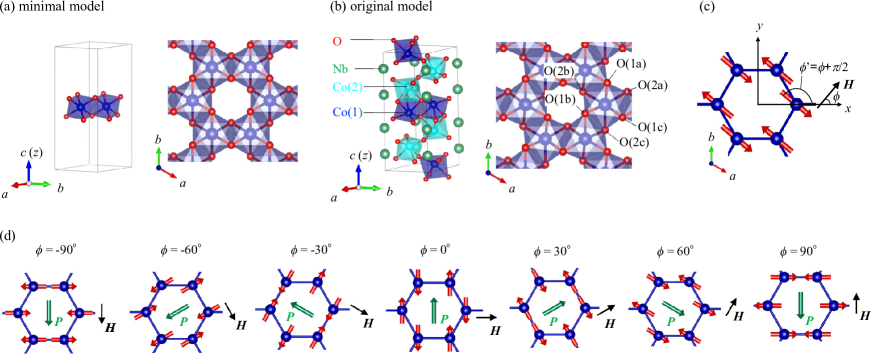
Figure 1: The lattice structures of (a) our minimal model and (b) original model for Co₄Nb₂O₉. (c) The AFM structure under the in-plane magnetic field $\bm{H}$. Note that $\bm{M}_{\mathrm{AFM}}$ is parallel to the $x$-axis in the absence of $\bm{H}$. (d) Schematic illustration of the induced electric polarization $\bm{P}$ and the AFM moment $\bm{M}_{\mathrm{AFM}}$ by rotating magnetic field $\bm{H}$ in the $xy$-plane.

In our previous study Yanagi , we have successfully reproduced the observed ME response on the basis of the realistic model derived from the density functional band calculation. However, the essential ingredients for such ME response remain unclear.

Let us begin with the minimal three-orbital model with $xy$-type SOC on the two-dimensional honeycomb lattice under the AFM molecular field. This model corresponds to the simplified one, in which we take into account the partially filled three orbitals $\ell=e_{g1},e_{g2},a_{1g}$ and the only single honeycomb layer composed of Co(1)O₆ octahedra in the original model for Co₄Nb₂O₉, and neglect the buckling structure [see Figs. 1(a) and (b)]. The Hamiltonian is given by

$$\mathcal{H}=\mathcal{H}_{\mathrm{kin}}+\mathcal{H}_{\mathrm{SOC}}+\mathcal{H}_{\mathrm{AFM}}.$$ (2)

Each term of $\mathcal{H}$ is explicitly given as follows,

$$\mathcal{H}_{\mathrm{kin}}=\sum_{\bm{k}\sigma}\sum_{\alpha\beta\ell\ell^{\prime}}H^{(0)}_{\alpha\ell\beta\ell^{\prime}}(\bm{k})d^{\dagger}_{\bm{k}\alpha\ell\sigma}d_{\bm{k}\beta\ell^{\prime}\sigma},$$ (3)

$$\mathcal{H}_{\mathrm{SOC}}=\frac{\lambda}{2}\sum_{\bm{k}\alpha}\sum_{\ell\ell^{\prime}\sigma\sigma^{\prime}}(l_{\ell\ell^{\prime}}^{x}\sigma^{x}_{\sigma\sigma^{\prime}}+l_{\ell\ell^{\prime}}^{y}\sigma^{y}_{\sigma\sigma^{\prime}})d^{\dagger}_{\bm{k}\alpha\ell\sigma}d_{\bm{k}\beta\ell^{\prime}\sigma^{\prime}},$$ (4)

$$\mathcal{H}_{\mathrm{AFM}}=-\Delta\sum_{\bm{k}\alpha\ell}\sum_{\sigma\sigma^{\prime}}p[\alpha]M_{\sigma\sigma^{\prime}}(\phi^{\prime})d^{\dagger}_{\bm{k}\alpha\ell\sigma}d_{\bm{k}\alpha\ell\sigma^{\prime}},$$

$$\quad\quad\quad\hat{M}(\phi^{\prime})=\cos\phi^{\prime}\hat{\sigma}^{x}+\sin\phi^{\prime}\hat{\sigma}^{y},$$ (5)

where $d^{(\dagger)}_{\bm{k}\alpha\ell\sigma}$ represents the annihilation (creation) operator for the electron on the sublattice $\alpha(=\mathrm{A},\mathrm{B})$ with wave vector $\bm{k}$, orbital $\ell$ and spin $\sigma(=\uparrow,\downarrow)$, and $\hat{\sigma}^{i}$ ($i=x,y$) represents $i$-th component of the Pauli matrix. $H^{(0)}_{\alpha\ell\beta\ell^{\prime}}(\bm{k})$ is the kinetic energy including the crystalline-electric-field (CEF) potential and nearest-neighbor hopping on the two-dimensional honeycomb lattice. Here, the Slater-Koster parametrization is used as $dd\sigma=-0.15\mathrm{eV}$, $dd\pi=(2/3)dd\sigma$, and $dd\delta=dd\sigma/6$. The CEF splitting is set to be $\varepsilon_{e_{g}}-\varepsilon_{a_{1g}}=0.62\mathrm{eV}$. The magnitudes of the SOC and the AFM molecular field are set as $\lambda=0.1\mathrm{eV}$ and $\Delta=2.0\mathrm{eV}$, respectively. These values are estimated from the density functional band calculation for Co₄Nb₂O₉ Yanagi . The factor $p[\alpha]=+1~{}(-1)$ for $\alpha=\mathrm{A}~{}(\mathrm{B})$ in Eq. (5) is used to represent the staggered order. There are 3 electrons per Co²⁺ ion, since we assumed that 4 of 7 electrons in Co²⁺ ion occupy the lowest $\varepsilon_{g}^{\prime}$ orbitals as will be discussed later. By the sufficiently large AFM molecular-field term $\mathcal{H}_{\rm AFM}$, the system becomes insulating. The explicit forms of the orbitals and orbital angular-momentum operators are given by (13) and (14), respectively. By diagonalizing the Hamiltonian in Eq. (2) at each $\bm{k}$, we obtain the energy bands $\varepsilon_{\bm{k}\zeta}$ and corresponding eigenvectors $|\bm{k}\zeta\rangle$ ($\zeta=1-12$).

We investigate the linear ME responses of the model Hamiltonian in Eq. (2) by means of the standard Kubo formula. Since the external magnetic field acts on both the spin and orbital magnetic moments, the ME tensor $\hat{\alpha}$ is a sum of the spin part $\hat{\alpha}^{S}$ and orbital part $\hat{\alpha}^{L}$, where $\hat{\alpha}^{L}$ is expressed by the correlation function between the velocity and orbital magnetic moment, $\hat{Q}^{L}(z)=\langle\langle V^{i};L^{j}\rangle\rangle_{z}$, as follows:

$$\hat{\alpha}^{L}=\lim_{\omega\rightarrow 0}\frac{\hat{Q}^{L}(\omega+i\eta)-\hat{Q}^{L}(i\eta)}{i\omega}.$$ (6)

Similarly, $\hat{\alpha}^{S}$ is obtained by replacing $L^{j}$ with $2S^{j}$. The velocity, orbital magnetic moment Thonhauser and spin magnetic moment operators are given by

$$V^{i}=\sum_{\bm{k}\sigma}\sum_{\alpha\beta\ell\ell^{\prime}}v^{i}_{\alpha\ell\beta\ell^{\prime}}(\bm{k})d^{\dagger}_{\bm{k}\alpha\ell\sigma}d_{\bm{k}\beta\ell^{\prime}\sigma},$$ (7)

$$L^{i}=\sum_{\bm{k}\alpha\sigma}\sum_{\ell\ell^{\prime}}l^{i}_{\ell\ell^{\prime}}d^{\dagger}_{\bm{k}\alpha\ell\sigma}d_{\bm{k}\alpha\ell^{\prime}\sigma},$$ (8)

$$S^{i}=\frac{1}{2}\sum_{\bm{k}\alpha\ell}\sum_{\sigma\sigma^{\prime}}\sigma^{i}_{\sigma\sigma^{\prime}}d^{\dagger}_{\bm{k}\alpha\ell\sigma}d_{\bm{k}\alpha\ell\sigma^{\prime}},$$ (9)

with $\hat{v}^{i}(\bm{k})=\partial\hat{H}^{(0)}(\bm{k})/\partial k_{i}$. The ME tensor $\alpha^{L}_{ij}$ in Eq. (6) is explicitly calculated as follows

$$\alpha^{L}_{ij}=\frac{1}{iV}\sum_{\bm{k}\zeta\zeta^{\prime}}\frac{\langle\bm{k}\zeta|V^{i}|\bm{k}\zeta^{\prime}\rangle\langle\bm{k}\zeta^{\prime}|L^{j}|\bm{k}\zeta\rangle}{\varepsilon_{\bm{k}\zeta}-\varepsilon_{\bm{k}\zeta^{\prime}}}\frac{f(\varepsilon_{\bm{k}\zeta})-f(\varepsilon_{\bm{k}\zeta^{\prime}})}{\varepsilon_{\bm{k}\zeta}-\varepsilon_{\bm{k}\zeta^{\prime}}+i\eta},$$ (10)

where $f(\varepsilon)=(e^{(\varepsilon-\mu)/T}+1)^{-1}$ is the Fermi distribution function with chemical potential $\mu$. By the above ME tensor, the induced electric polarization is expressed as $P_{i}/H=\alpha_{ix}\sin\phi^{\prime}-\alpha_{iy}\cos\phi^{\prime}$.

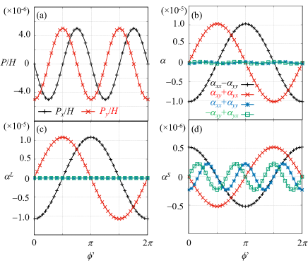
Figure 2: Angle $\phi^{\prime}$-dependence of $\bm{P}$ and $\hat{\alpha}$ at $T=0.01$eV. (a) electric polarization $\bm{P}$, (b) total ME tensor $\alpha_{ij}=\alpha^{S}_{ij}+\alpha^{L}_{ij}$, (c) orbital part $\alpha^{L}_{ij}$, and (d) spin part $\alpha^{S}_{ij}$.

Figure 2(a) shows the $\phi^{\prime}$-dependence of the electric polarization $\bm{P}$. It is found that $\bm{P}\propto(-\sin 2\phi^{\prime},-\cos 2\phi^{\prime})$, which is consistent with the observed behavior. The $\phi^{\prime}$-dependences of $\alpha_{ij}$, $\alpha^{L}_{ij}$ and $\alpha^{S}_{ij}$ are also shown in Figs. 2(b), (c) and (d), respectively. In our minimal model, $\hat{\alpha}^{L}$ dominates over $\hat{\alpha}^{S}$. The orbital part $\hat{\alpha}^{L}$ has only the fundamental $\phi^{\prime}$ rotation, which is characterized by $r_{L}\sim 1$ in Eq. (1), while the spin part $\hat{\alpha}^{S}$ has both $\phi^{\prime}$ and $3\phi^{\prime}$ rotations characterized by $r_{S}\sim 0.0244$. In total, $\hat{\alpha}$ is characterized by $r\sim 1.027$, indicating that magnetic quadrupoles play a dominant role in ME for Co₄Nb₂O₉.

Next, we discuss the connection between our minimal model and the realistic model for Co₄Nb₂O₉. In Co₄Nb₂O₉, O^2--ions form a trigonally distorted octahedron around a Co-atom as shown in Fig. 1(b). The CEF from O^2--ions splits $3d$ orbitals of a Co-atom into the non-degenerate $a_{1g}$ orbital and two sets of doubly degenerate $e_{g}$ and $e_{g}^{\prime}$ orbitals. The wave functions of the $e_{g}$ and $a_{1g}$ orbitals are given by

$$|e_{g1}\rangle=\frac{2}{\sqrt{6}}|yz\rangle-\frac{1}{\sqrt{3}}|x^{2}-y^{2}\rangle,$$ (11)

$$|e_{g2}\rangle=-\frac{2}{\sqrt{6}}|zx\rangle+\frac{1}{\sqrt{3}}|xy\rangle,$$ (12)

$$|a_{1g}\rangle=|3z^{2}-r^{2}\rangle.$$ (13)

According to the first principles band calculations, the CEF level scheme is as follows, $\varepsilon_{e_{g}}>\varepsilon_{a_{1g}}>\varepsilon_{e_{g}^{\prime}}$, where $\varepsilon_{\ell}$ is the atomic energy of the orbital $\ell$ CEF_band . By considering the electron configuration of Co²⁺ ions, $(3d)^{7}$, we assume that the lowest lying $e_{g}^{\prime}$ orbitals are fully occupied, and the rest of $e_{g}$ and $a_{1g}$ orbitals are partially filled by 3 electrons. Within these orbital space, the matrix elements of the orbital angular-momentum operators are given by

$$\hat{l}^{x}=\sqrt{2}\begin{pmatrix}0&0&-i\\ 0&0&0\\ i&0&0\end{pmatrix},\quad\hat{l}^{y}=\sqrt{2}\begin{pmatrix}0&0&0\\ 0&0&-i\\ 0&i&0\end{pmatrix},$$ (14)

and $\hat{l}^{z}$ vanishes. As a result, the SOC in our minimal model, Eq. (4), is the $xy$-type.

Up to this point, the minimal ingredients to exhibit the in-plane ME response as Eq. (1) are given. So that further differences between our minimal model and the realistic model for Co₄Nb₂O₉ do not play any important roles in the occurrence of the in-plane ME response. We summarize the differences as follows. In the original lattice structure, the unit cell contains four sets of the two distinct Co-atoms, Co(1) and Co(2) and the edge-shared (corner-shared) Co(1)O₆ [Co(2)O₆] octahedra form buckled honeycomb structures as shown in Fig. 1(b). Here, we note that in a Co(1)O₆ octahedron, the triangle formed by three O-atoms located on the upper plane of a Co(1)-atom, O(1a)-O(1c), and that formed by O-atoms on the lower plane, O(2a)-O(2c), are not equivalent to each other as shown in Fig. 1(b). In our minimal model, we assume that the upper triangle, O(1a)-O(1c), and the lower triangle, O(2a)-O(2c), are equivalent, and there are additional two-fold rotational symmetries along the nearest neighbor Co(1)-Co(1) bonds, [see Fig. 1(a)]. Accordingly, the point-group symmetry of the single Co(1) honeycomb layer in our minimal model is upgraded from the original $C_{3i}$ group to higher $D_{3d}$ group.

Finally, we discuss that the obtained ME response in our minimal model is naturally understood by the perturbative calculation with respect to the atomic SOC. Likewise magnetic susceptibility, one can calculate the correlation function $Q^{L(S)}_{ij}(i\nu_{m})$ by the Green’s function technique in Matsubara framework, and obtain $Q^{L(S)}_{ij}(\omega+i\eta)$ in Eq. (6) by the analytic continuation procedure, $i\nu_{m}\rightarrow\omega+i\eta$, where $\nu_{m}=2m\pi T$ is the bosonic Matsubara frequency. By the formal expansion of the non-perturbative Green’s function $\hat{G}(k)$ in terms of $\hat{G}_{0}^{-1}(k)=(i\omega_{n}+\mu)\hat{1}-\hat{H}^{0}(\bm{k})$ with respect to the AFM molecular-field term, $-\Delta\hat{M}(\phi^{\prime})\hat{\rho}^{z}$ with $\hat{\rho}^{z}$ being the $z$-component of the Pauli matrix in the sublattice space, we obtain

$$\hat{G}(k)= \hat{G}_{0}-\Delta\hat{G}_{0}\hat{M}\hat{\rho}^{z}\hat{G}_{0}+\Delta^{2}\hat{G}_{0}(\hat{M}\hat{\rho}^{z}\hat{G}_{0})^{2}-\cdots$$ (15)

$$= \hat{G}_{0}[\hat{1}-\Delta^{2}(\hat{\rho}^{z}\hat{G}_{0})^{2}]^{-1}$$ (16)

$$\quad-\Delta\hat{M}\hat{G}_{0}\hat{\rho}^{z}\hat{G}_{0}[\hat{1}-\Delta^{2}(\hat{\rho}^{z}\hat{G}_{0})^{2}]^{-1}$$ (17)

$$= \hat{G}_{\mathrm{E}}(k)+\hat{M}(\phi^{\prime})\hat{G}_{\mathrm{O}}(k),$$ (18)

where we have introduced the diagonal and off-diagonal Green’s functions, $\hat{G}_{\rm E}$ and $\hat{G}_{\rm O}$, in the spin space as

$$\hat{G}_{\mathrm{E}}(k)=[\hat{G}_{0}^{-1}(k)-\Delta^{2}\hat{\rho}^{z}\hat{G}_{0}(k)\hat{\rho}^{z}]^{-1},$$ (19)

$$\hat{G}_{\mathrm{O}}(k)=-\Delta\hat{G}_{0}(k)\hat{\rho}^{z}\hat{G}_{\mathrm{E}}(k).$$ (20)

Here, $k=(\bm{k},i\omega_{n})$ with the fermionic Matsubara frequency, $\omega_{n}=(2n+1)\pi T$, and we have used the facts that $\hat{\rho}^{z}\hat{G}_{0}$ and $\hat{M}$ are commutable, and $\hat{M}^{2}=\hat{1}$.

From Eq. (18), it is found that the angle-dependence of the AFM moment $\hat{M}(\phi^{\prime})$ appears as the prefactor of $\hat{G}_{\mathrm{O}}(k)$. This $\phi^{\prime}$-dependence is reflected on the ME tensor through the atomic SOC.

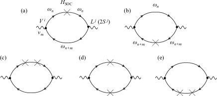
Figure 3: The diagrammatic representation of the correlation function $Q^{L(S)}_{ij}(i\nu_{m})$. The first and second order terms with respect to the atomic SOC are shown in (a) and (b), and (c)-(e), respectively. The arrows and crosses represent the non-perturbative Green’s function $\hat{G}(k)$ and the SOC term $\mathcal{H}_{\mathrm{SOC}}$, respectively. $Q^{L(S)}_{ij}(\omega+i\eta)$ is obtained by the analytic continuation, $i\nu_{m}\to\omega+i\eta$, in $Q^{L(S)}_{ij}(i\nu_{m})$.

Let us consider the first-order terms of the ME tensor with respect to the atomic SOC, $Q^{L(S)(1)}_{ij}(i\nu_{m})$, which can be expressed as products of $V^{i}$, $L^{j}(S^{j})$, $\mathcal{H}_{\mathrm{SOC}}$, and the three Green’s functions $\hat{G}(k)$. The corresponding diagrammatic representations are shown in Figs. 3(a) and (b). In what follows, the symmetry arguments are useful to identify which perturbative terms remain finite. For instance, the spin-diagonal Green’s function $\hat{G}_{\mathrm{E}}(k)$ is even-parity, while the spin-off-diagonal $\hat{G}_{\mathrm{O}}(k)$ is odd-parity due to the additional $\hat{\rho}^{z}$ in the latter. Therefore, by considering the fact that $V^{i}$ is odd-parity, while $L^{i}$, $S^{i}$, and $\mathcal{H}_{\mathrm{SOC}}$ are even-parity, the perturbative terms containing odd numbers of $\hat{G}_{\mathrm{O}}(k)$ remain finite. Moreover, $\mathcal{H}_{\mathrm{SOC}}$ in Eq. (4), $S^{i}$ in Eq. (9), and $\hat{M}$ in Eq. (18) contain $\hat{\sigma}^{x}$ and $\hat{\sigma}^{y}$, but their products appeared in the perturbative terms must be spin independent, otherwise they vanish due to the trace over the spin indices. As a result, $Q^{S(1)}_{ij}(i\nu_{m})$ vanishes, while $Q^{L(1)}_{ij}(i\nu_{m})$ is given as

$$\frac{Q^{L(1)}_{ij}(i\nu_{m})}{\lambda}=\left(I_{ij}^{x}+J_{ij}^{x}\right)\cos\phi^{\prime}+\left(I_{ij}^{y}+J_{ij}^{y}\right)\sin\phi^{\prime},$$ (21)

$$\quad I_{ij}^{k}(i\nu_{m})=-\int_{k}\mathrm{tr}\left[\hat{v}^{i}(\bm{k})\hat{G}_{\mathrm{P}_{1}}(k_{+})\hat{l}^{j}\hat{G}_{\mathrm{P}_{2}}(k)\hat{l}^{k}\hat{G}_{\mathrm{P}_{3}}(k)\right],$$ (22)

$$\quad J_{ij}^{k}(i\nu_{m})=-\int_{k}\mathrm{tr}\left[\hat{v}^{i}(\bm{k})\hat{G}_{\mathrm{P}_{1}}(k_{+})\hat{l}^{k}\hat{G}_{\mathrm{P}_{2}}(k_{+})\hat{l}^{j}\hat{G}_{\mathrm{P}_{3}}(k)\right],$$ (23)

where we have introduced the abbreviation, $\int_{k}\equiv(T/N)\sum_{\bm{k}n}\sum_{\mathrm{P}_{1}\mathrm{P}_{2}\mathrm{P}_{3}}$ where $\mathrm{P}_{r}$ takes either E or O, and $k_{+}=(\bm{k},i\omega_{n+m})$. As was mentioned, the only odd number of O in the summation ($\mathrm{P}_{1},\mathrm{P}_{2},\mathrm{P}_{3})$ gives finite contributions. The trace $\mathrm{tr}[\cdots]$ is taken over the orbital and sublattice indices. Furthermore, the point-group argument concludes the following relations: $-I_{xx}^{x}=I_{yy}^{x}=I_{xy}^{y}=I_{yx}^{y}=A(i\nu_{m})$, and the other components vanish. Similar relations also hold for $J^{k}_{ij}$. By these arguments, the first-order contribution is purely from the orbital part, and $\hat{\alpha}$ follows Eq. (1) with $r=1$. Similar arguments can be applied to the second-order terms as shown in Figs. 3(c)-(e). It is found that the orbital contribution vanishes, while $\hat{\alpha}^{S}$ contains both $\phi^{\prime}$ and $3\phi^{\prime}$ rotations, i.e., $r\neq 0$, $1$ in Eq. (1).

In summary, we have proposed a minimal model to exhibit the manipulating in-plane ME by extracting minimal ingredients from the realistic model for Co₄Nb₂O₉. The minimal conditions are (i) three $d$ orbitals in a trigonally distorted octahedron giving rise to the $xy$-type SOC, (ii) single honeycomb layer with weak in-plane magnetic anisotropy, and (iii) weak SOC $\lambda$ as compared to AFM molecular field $\Delta$. The $\bm{H}$-angle-dependence of the electric polarization in our minimal model is qualitatively consistent with experiments, and is understood by the perturbative argument with respect to $\lambda/\Delta$. Our results can be applied to other AFMs, e.g., Co₄Ta₂O₉, showing the similar ME response. These findings could be useful to explore efficiently further ME materials having similar manipulability of the electric polarization.

- (1) Y. Tokura and N. Nagaosa, Science 288, 462 (2000).
- (2) S. Murakami, N. Nagaosa, and S. C. Zhang, Science 301, 1348 (2003).
- (3) M. Z. Hasan and C. L. Kane, Rev. Mod. Phys. 82, 3045 (2010).
- (4) A. Rycerz, J. Tworzydło, and C. W. Beenakker, Nat. Phys. 3, 172 (2007).
- (5) P. Curie, J. Phys. Theor. Appl. 3, 393 (1894).
- (6) I. E. Dzyaloshinskii, Sov. Phys. JETP 10, 628 (1960).
- (7) D. N. Astrov, Sov. Phys. JETP 11, 708 (1960).
- (8) T. Kimura, T. Goto. H. Shintani, K. Ishizaka, T. Arima, and Y. Tokura, Nature 426, 55 (2003).
- (9) H. Katsura, N. Nagaosa, and A. V. Balatsky, Phys. Rev. Lett. 95, 057205 (2005).
- (10) M. Mostovoy, Phys. Rev. Lett. 96, 067601 (2006).
- (11) I. A. Sergienko and E. Dagotto, Phys. Rev. B 73, 094434 (2006).
- (12) S.-W. Cheong and M. Mostovoy, Nat. Mater. 6, 13 (2007).
- (13) D. Khomskii, Physics 2, 20 (2009).
- (14) T. Arima, J. Phy. Soc. Jpn. 80, 052001 (2011).
- (15) M. Fiebig, J. Phys. D 38, R123 (2005).
- (16) N. A. Spaldin, M. Fiebig, and M. Mostovoy, J. Phys.: Condens. Matter 20, 434203 (2008).
- (17) J. Íñiguez, Phys. Rev. Lett. 101, 117201 (2008).
- (18) A. Malashevich, S. Coh, I. Souza, and D. Vanderbilt, Phys. Rev. B 86, 094430 (2012).
- (19) A. Scaramucci, E. Bousquet, M. Fechner, M. Mostovoy, and N. A. Spaldin, Phys. Rev. Lett. 109, 197203 (2012).
- (20) S. Picozzi and A. Stroppa, Eur. Phys. J. B 85, 240 (2012).
- (21) Y. Yanase, J. Phys. Soc. Jpn. 83, 014703 (2014).
- (22) H. Watanabe and Y. Yanase, Phys. Rev. B 96, 064432 (2017).
- (23) S. Hayami, H. Kusunose, and Y. Motome, Phys. Rev. B 90, 024432 (2014).
- (24) S. Hayami, H. Kusunose, and Y. Motome, Phys. Rev. B 90, 081115(R) (2014).
- (25) S. Hayami, H. Kusunose, and Y. Motome, J. Phys.: Condens. Matter 28, 395601 (2016).
- (26) Y. Kato, K. Kimura, A. Miyake, M. Tokunaga, A. Matsuo, K. Kindo, M. Akaki, M. Hagiwara, M. Sera, T. Kimura, and Y. Motome, Phys. Rev. Lett. 118, 107601 (2017).
- (27) E. Ascher, H. Rieder, H. Schmid, and H. Stössel, J. Appl. Phys. 37, 1404 (1966).
- (28) N. D. Khanh, Ph. D thesis, Tohoku University (2015).
- (29) N. D. Khanh, N. Abe, S. Kimura, Y. Tokunaga, and T. Arima, Phys. Rev. B 96, 094434 (2017).
- (30) E. Fischer, G. Gorodetsky, and R. M. Hornreich, Solid State Commun. 10, 1127 (1972).
- (31) E. F. Bertaut, L. Corliss, F. Forrat, R. Aleonard, and R. Pauthenet, J. Phys. Chem. Solids 21, 234 (1961).
- (32) M. A. R. Castellanos, S. Bernès, and M. Vega-González, Acta Crystallogr. Sect. E 62, i117 (2006).
- (33) T. Kolodiazhnyi, H. Sakurai, and N. Vittayakorn, Appl. Phys. Lett. 99, 132906 (2011).
- (34) Y. Fang, Y. Q. Song, W. P. Zhou, R. Zhao, R. J. Tang, H. Yang, L. Y. Lv, S. G.Yang, D. H. Wang, and Y. W. Du, Sci. Rep. 4, 3860 (2014).
- (35) N. D. Khanh, N. Abe, H. Sagayama, A. Nakao, T. Hanashima, R. Kiyanagi, Y. Tokunaga, and T. Arima, Phys. Rev. B 93, 075117 (2016).
- (36) G. Denga, Y. Cao, W. Ren, S. Cao, A. J. Studera, N. Gauthier, M. Kenzelmann, G. Davidson, K. C. Rule, J. S. Gardner, P. Imperia, C. Ulrich, G. J. McIntyre, arXiv: 1705.04017.
- (37) I. V. Solovyev and T. V. Kolodiazhnyi, Phys. Rev. B 94, 094427 (2016).
- (38) Y. Yanagi, S. Hayami, and H. Kusunose, Proceedings of SCES 2017 in Physica B (in press).
- (39) In ref. Yanagi , the CEF splittings, ()eV and ()eV at a Co(1) [Co(2)] site have been obtained from the band calculation. These values are somewhat different from those in ref. Solovyev . This is mainly because the different structural parameters were used, namely, ref. Castellanos was used in ref. Solovyev , and Bertaut was used in ref. Yanagi .
- (40) In the present work, we took into account the local contributions of the orbital momentum. This treatment is approximate. For rigorous treatment, one should take into account the itinerant circular contribution, see T. Thonhauser, D. Ceresoli, D. Vanderbilt, and R. Resta, Phys. Rev. Lett. 95, 137205 (2005).