Calculating eigenvalues of many-body systems from partition functions

Abstract

A method for calculating the eigenvalue of a many-body system without solving the eigenfunction is suggested. In many cases, we only need the knowledge of eigenvalues rather than eigenfunctions, so we need a method solving only the eigenvalue, leaving alone the eigenfunction. In this paper, the method is established based on statistical mechanics. In statistical mechanics, calculating thermodynamic quantities needs only the knowledge of eigenvalues and then the information of eigenvalues is embodied in thermodynamic quantities. The method suggested in the present paper is indeed a method for extracting the eigenvalue from thermodynamic quantities. As applications, we calculate the eigenvalues for some many-body systems. Especially, the method is used to calculate the quantum exchange energies in quantum many-body systems. Using the method, we also calculate the influence of the topological effect on eigenvalues. Moreover, we improve the result of the relation between the counting function and the heat kernel in literature.

1 Introduction

Calculating the eigenvalue of a many-body system is often difficult. The most direct way is to solve the eigenequation of the Hamiltonian $H$,

$$H\left|\phi_{n}\right\rangle=E_{n}\left|\phi_{n}\right\rangle.$$ (1.1)

Once the eigenequation is solved, both the eigenvalue $E_{n}$ and the eigenfunction $\phi_{n}$ are solved simultaneously. Nevertheless, often one only needs the knowledge of eigenvalues $\{E_{n}\}$ rather than eigenfunctions. In such cases, solving eigenfunctions is redundant. This inspires us to develop an approach which only focus on solving eigenvalues.

Statistical mechanics is essentially an averaging method. In statistical mechanics the information of eigenfunctions is statistically averaged out; calculating thermodynamic quantities needs only eigenvalues. For example, in canonical ensembles, all the thermodynamic property of an $N$-particle system is embodied in the canonical partition function which is determined only by eigenvalues $\{E_{n}\}$:

$$Z\left(\beta\right)=\sum_{n}e^{-\beta E_{n}},$$ (1.2)

where $\beta=\frac{1}{kT}$ with $k$ the Boltzmann constant and $T$ the temperature.

The knowledge of eigenvalues is embodied in the canonical partition function $Z\left(\beta\right)$. Our problem is how to extract the eigenvalue $E_{n}$ from the partition function (1.2), or, more generally, from thermodynamic quantities.

The canonical partition function (1.2), from another perspective, is the global heat kernel of the Hamiltonian operator $H$. The global heat kernel

$$K\left(t\right)=\sum_{n}e^{-tE_{n}}$$ (1.3)

is the trace of the local heat kernel which is the Green function of the initial-value problem of the heat-type equation [1]. Obviously, the global heat kernel is just the canonical partition function with the replacement $t\rightarrow\beta$.

Recently, a relation between the heat kernel and the spectral counting function is revealed [2, 3]. The counting function $N\left(E\right)$ counts the number of the eigenstates whose eigenvalues are smaller than $E$. The relation between the heat kernel and the counting function allows us to calculate the counting function $N\left(E\right)$ from the heat kernel $K\left(t\right)$, or, the canonical partition function $Z\left(\beta\right)$, directly.

The eigenvalue can be calculated from the counting function $N\left(E\right)$ [2]. This implies that one can calculate the eigenvalue from the canonical partition function $Z\left(\beta\right)$ or other thermodynamic quantities.

It is often difficult to calculate the eigenvalue of noninteracting quantum systems and interacting classical and quantum systems. In noninteracting quantum systems, there exist quantum exchange interactions; in classical interacting systems, there exist classical inter-particle interactions, and in quantum interacting systems, there exist both classical inter-particle interactions and quantum exchange interactions [4]. The method developed in the present paper allows us to calculated eigenvalues from the thermodynamic quantity which is obtained by the statistical mechanical method.

In quantum many-body systems, the most important factor is the quantum exchange interaction. The effect of quantum exchange interaction in eigenvalue is the exchange energy. In statistical mechanics, the quantum exchange effect is taken into account by simply employing Bose-Einstein statistics, Fermi-Dirac statistics, and various kinds of intermediate statistics through imposing various maximum occupation numbers: $\infty$ for Bose-Einstein statistics, $1$ for Fermi-Dirac statistics, and an integer $n$ for Gentile statistics [5, 6, 7, 8, 9, 10, 11, 12]. The method suggested in the present paper allows us to calculate the exchange energy in eigenvalues from the partition function obtained in statistical mechanics. In other words, we can calculate the exchange energy in virtue of the statistical mechanics. For example, in quantum ideal and interacting gases, the contribution of the exchange energy to the eigenvalue is represented by the second virial coefficient which can be obtained by statistical mechanical method.

In quantum mechanics, the exchange energy is reckoned in by symmetrizing or antisymmetrizing the wavefunctions, in quantum filed theory, the exchange energy is reckoned in by imposing the quantization condition on the fields, while, in statistical mechanics, the exchange energy is reckoned in by only simply setting the value of the maximum occupation number, since in statistical mechanics only the information of eigenvalues other than the information of wavefunctions is needed. That is to say, in statistical mechanics, the exchange energy can be calculated relatively simply. Therefore, calculating the exchange energy through statistical mechanics is a more simple approach.

Moreover, using the method, we calculate the influence of the topological effect on eigenvalues for two-dimensional non-interacting classical and quantum systems. In two-dimensional systems, the topological property is described by connectivity which is described by the Euler-Poincaré characteristic number [13].

In statistical mechanics, there are many solved models, in which the partition functions are solved exactly or approximately. Using the method, we calculate the eigenvalues for such models from the solved partition functions. In this paper, we consider classical and quantum non-interacting systems, classical interacting systems with the Lennard-Jones interaction and quantum interacting systems with the hard-sphere interaction, the one-dimensional Ising models, and the one-dimensional Potts model.

There are many studies devoted to the problem of eigenvalue spectra, such as the eigenvalue spectrum of the Rabi model [14], the eigenvalue spectrum of the open spin-1/2 XXZ quantum chains with non-diagonal boundary terms [15], the eigenvalue spectrum of the antiperiodic spin-1/2 XXZ quantum chains [16], the statistical property of the eigenvalue spectrum [17, 18], the structure of the eigenvalue spectrum [19, 20], the ground-state energy of the Heisenberg-Ising lattice [21], the ground state and the excited state of many-body localized Hamiltonians [22], and the ground state energy of a system of $N$ bosons [23].

In statistical mechanics, many methods are developed for the calculation of partition functions. For example, the canonical partition function for quon statistics [24], general formulas for the canonical partition function of parastatistical systems [25], the canonical partition function of the freely jointed chain model [26], the partition function of the interacting calorons ensemble [27], the algorithm for computing the exact partition function of lattice polymer models [28], the exact partition function for the $q$-state Potts Model [29], the partition function for the antiferromagnetic Ising model and the hard-core models [30], and the canonical partition functions for different gaseous systems [31] are investigated.

The relation between the counting function and the heat kernel is the basics of the method used in the present paper. However, the relation given by Ref. [2] neglects a special case. In this paper, we improve the result in Ref. [2].

This paper is organized as follows. In section 2, we describe the method of calculating the eigenvalue from the canonical partition function. In section 3, we illustrate the method by examples. In sections 4 and 5, we calculate the eigenvalue, especially the exchange energy, of identical particles in a box and in an external field. In section 6, we calculate the influence of the topological effect on eigenvalues. In sections 7 and 8, we calculate the eigenvalue of interacting particles with the Lennard-Jones potential and the hard-sphere potential. In sections 9 and 10, we calculate the eigenvalues of the Ising system and the Potts system. Conclusions are summarized in section 11. In the appendix, we provide a complete result for the relation between the counting function and the heat kernel.

2 Calculating eigenvalues from partition functions

In mechanics, all the dynamical informations are embodied in the Hamiltonian $H$.

When regarding a many-body system as a mechanical system, one describes the system by the solution of the eigenequation $H\left|\phi_{n}\right\rangle=E_{n}\left|\phi_{n}\right\rangle$. The solution of the eigenfunction, the eigenvalues $E_{n}$ and the eigenvectors $\left|\phi_{n}\right\rangle$, contains all the informations of the Hamiltonian $H$. In fact, the Hamiltonian $H$ can be reconstructed by the spectral representation as $H=\sum_{n}E_{n}\left|\phi_{n}\right\rangle\left\langle\phi_{n}\right|$.

When solving an eigenequation is difficult, we can regard a many-body system as a thermodynamic system paying the price of losing the information of the eigenvectors $\left|\phi_{n}\right\rangle$. A thermodynamic system can be completely described by, e.g., in canonical ensembles, the partition function $Z\left(\beta\right)=\operatorname*{tr}e^{-\beta H}$. In a thermodynamic description, only the information is taken into account and the information of the wavefunction are averaged out.

In a word, any mechanical system corresponds a thermodynamic system which reserves only the information of eigenvalues. Although the information of the wavefunction is lost in the thermodynamic description, the information of eigenvalues remains. If we can extract the information of eigenvalues from the thermodynamic quantity, we arrive at an approach solving only eigenvalues without solving wavefunctions in the meantime. In this section, we show how to calculate the eigenvalue of a system from the corresponding canonical partition function in statistical mechanics.

For an eigenvalue spectrum $\left\{E_{n}\right\}$, the spectral counting function $N\left(E\right)$ describes how many eigenstates whose eigenvalues are smaller than $E$. In Refs. [2, 3], a relation between the spectral counting function $N\left(E\right)$ and the global heat kernel $K\left(t\right)$ is given: $N\left(E\right)=\frac{1}{2\pi i}\int_{c-i\infty}^{c+i\infty}\frac{K\left(t\right)}{t}e^{tE}dt$. By the relation between the global heat kernel $K\left(t\right)$ and the canonical partition function $Z\left(\beta\right)$, we can calculate the counting function $N\left(E\right)$ from the canonical partition function $Z\left(\beta\right)$:

$$N\left(E\right)=\frac{1}{2\pi i}\int_{c-i\infty}^{c+i\infty}\frac{Z\left(\beta\right)}{\beta}e^{\beta E}d\beta.$$ (2.1)

The $n$-th eigenvalue $E_{n}$ can be obtained from the counting function by the equation [32]

$$N\left(E_{n}\right)=n.$$ (2.2)

Consequently, the eigenvalue $E_{n}$ can be solved by the following equation:

$$\frac{1}{2\pi i}\int_{c-i\infty}^{c+i\infty}\frac{Z\left(\beta\right)}{\beta}e^{\beta E_{n}}d\beta=n.$$ (2.3)

In the following, we solve eigenvalues for some many-body systems from the corresponding canonical partition functions.

In should be emphasized that, in the relation between the counting function and the heat kernel (canonical partition function), Eq. (2.1), there is a constant term $-\frac{1}{2}$ when $E=E_{n}$, (see Appendix A). We will not take the contribution into account, because its influence is often small enough to be ignored, especially for highly-excited states, .

3 Illustration of the method

In this section, we illustrate the method by some models whose eigenvalues are already known, including a particle in a box, a harmonic oscillator, and $N$ bosonic harmonic oscillators.

3.1 A particle in a box

A particle in a box in quantum mechanics corresponds to a classical ideal gas confined in a box in statistical mechanics.

In the following, we illustrate the method by calculating the eigenvalue of a particle in a box in virtue of the canonical partition function of a classical ideal gas confined in a box.

In classical ideal gases, there are no classical inter-particle interactions and quantum exchange interactions. The canonical partition function of a classical ideal gas consisting of $N$ particles is [33]

$$Z\left(\beta\right)=z^{N}\left(\beta\right),$$ (3.1)

where $z\left(\beta\right)$ is the single-particle partition function. The single-particle partition function for free particles is [33]

$$z\left(\beta\right)=\frac{V}{\lambda^{D}},$$ (3.2)

where $\lambda=h\sqrt{\frac{\beta}{2\pi m}}$ is the thermal wavelength with $m$ the mass of the particle and $h$ the Planck constant, $V$ is the volume of the container, and $D$ is the spatial dimension. The canonical partition function of an $N$-particle classical ideal gas, by Eqs. (3.2) and (3.1), is then

$$Z\left(\beta\right)=\left(\frac{V}{\lambda^{D}}\right)^{N}.$$ (3.3)

By the relation between the counting function $N\left(\lambda\right)$ and the canonical partition function $Z\left(\beta\right)$, Eq. (2.1), we can obtain the counting function,

$$N\left(E_{n}^{cl}\right)=V^{N}\left(\frac{2\pi m}{h^{2}}\right)^{DN/2}\frac{1}{\Gamma\left(1+DN/2\right)}\left(E_{n}^{cl}\right)^{DN/2},$$ (3.4)

where $\Gamma\left(x\right)$ is the Gamma function. The eigenvalue is determined by the equation obtained by substituting Eq. (3.4) into Eq. (2.2):

$$V^{N}\left(\frac{2\pi m}{h^{2}}\right)^{DN/2}\frac{1}{\Gamma\left(1+DN/2\right)}\left(E_{n}^{cl}\right)^{DN/2}=n.$$ (3.5)

Solving the equation gives the eigenvalue

$$E_{n}^{cl}=\frac{h^{2}}{2\pi mV^{2/D}}\Gamma^{2/\left(DN\right)}\left(1+\frac{DN}{2}\right)n^{2/\left(DN\right)}.$$ (3.6)

Now let us see a familiar special case: the one-dimensional single-particle case. In this case, $D=1$, $N=1$, and $V=L$. Eq. (3.6) then becomes

$$\left.E_{n}^{cl}\right|_{N=1}=\frac{h^{2}}{8m}\left(\frac{n}{L}\right)^{2}.$$ (3.7)

This is just the eigenvalue of a particle in a one-dimensional periodic box with a side length $L$. In a one-dimensional periodic box with a side length $L$, the momentum of the particle is $p_{n}=\frac{h}{2L}n$, so the eigenvalue (3.7) becomes

$$\left.E_{n}^{cl}\right|_{N=1}=\frac{p_{n}^{2}}{2m}.$$ (3.8)

3.2 One harmonic oscillator

The harmonic oscillator in quantum mechanics corresponds to a classical ideal harmonic oscillator gas in statistical mechanics.

In order to show the validity of the method and illustrate the method, we take the harmonic oscillator as an example.

The eigenvalue of a harmonic oscillator is exactly known: $E_{n}=\hbar\omega\left(n+\frac{1}{2}\right)$. The corresponding partition function is

$$Z\left(\beta\right)=\sum_{n=1}^{\infty}e^{-\beta\hbar\omega\left(n+\frac{1}{2}\right)}=\left(e^{\frac{1}{2}\beta\hbar\omega}-e^{-\frac{1}{2}\beta\hbar\omega}\right)^{-1}.$$ (3.9)

Now we show how to obtain the eigenvalue from the partition function by the method.

By the relation between the counting function $N\left(E_{n}\right)$ and the canonical partition function $Z\left(\beta\right)$, Eq. (2.1), we can obtain the counting function.

First expand partition function (3.9) in power series of $e^{-\beta\hbar\omega}$,

$$Z\left(\beta\right)=\sum_{k=1}^{\infty}e^{-\frac{1}{2}\beta\hbar\omega}e^{-\beta\hbar\omega k}.$$ (3.10)

Substituting Eq. (3.10) into Eq. (2.1) gives the counting function:

$$N\left(E\right)=\sum_{k=1}^{\infty}\theta\left(E-\left(\frac{1}{2}+k\right)\hbar\omega\right),$$ (3.11)

where $\theta\left(x\right)$ is the Heaviside theta function. The eigenvalue is determined by $N\left(E_{n}\right)=n$, which directly gives the eigenvalue of a harmonic oscillator:

$$E_{n}=\hbar\omega\left(n+\frac{1}{2}\right).$$ (3.12)

3.3 $N$ bosonic harmonic oscillators

An $N$ bosonic harmonic oscillator system in quantum mechanics corresponds to a bosonic harmonic oscillator gas in statistical mechanics.

In this example, we show the validity of the method.

3.3.1 Calculating eigenvalues from partition functions

The exact canonical partition function of a system consists of $N$ bosonic harmonic oscillators is given by [31]

$$Z\left(\beta,N\right)=\frac{1}{N!}\det\left(\begin{array}[c]{ccccc}Z\left(\beta\right)&-1&0&...&0\\ Z\left(2\beta\right)&Z\left(\beta\right)&-2&...&0\\ Z\left(3\beta\right)&Z\left(2\beta\right)&Z\left(\beta\right)&...&...\\ ...&...&...&...&-\left(N-1\right)\\ Z\left(N\beta\right)&Z\left(N\beta-\beta\right)&Z\left(N\beta-2\beta\right)&...&Z\left(\beta\right)\end{array}\right).$$ (3.13)

where $Z\left(\beta\right)$ is the single particle partition function given by Eq. (3.9).

As examples, consider two cases: $N=2$ and $N=3$.

Exact eigenvalues

For $N=2$, the partition function given by Eq. (3.13) reads

$$Z\left(\beta,2\right)=\frac{e^{2\hbar\omega\beta}}{\left(e^{\hbar\omega\beta}-1\right)^{2}\left(e^{\hbar\omega\beta}+1\right)}.$$ (3.14)

Expanding $Z\left(\beta,2\right)$ given by Eq. (3.14) as a power series of $e^{-\beta\hbar\omega}$ gives

$$Z\left(\beta,2\right)=\sum_{k=1}\frac{1}{4}\left[2k+1-\left(-1\right)^{k}\right]\left(e^{-\hbar\omega\beta}\right)^{k}.$$ (3.15)

The counting function can be obtained by substituting Eq. (3.15) into Eq. (A.4):

$$N\left(E\right)=\sum_{k=1}\frac{1}{4}\left[2k+1-\left(-1\right)^{k}\right]\theta\left(E-k\hbar\omega\right),$$ (3.16)

The eigenvalue can be obtained by solving Eq. (2.2). It can be directly shown that the exact solution of Eq. (2.2) with the counting function (3.16) is

$$E^{N=2}=\left(n+1\right)\hbar\omega$$ (3.17)

with the degeneracy

$$\omega\left(E^{N=2}\right)=\frac{1}{4}\left[3+\left(-1\right)^{n}+2n\right].$$ (3.18)

This agrees with the exact result given in Ref. [34].

For $N=3$, the partition function given by Eq. (3.13) reads

$$Z\left(\beta,3\right)=\frac{e^{9\hbar\omega\beta/2}}{\left(e^{\hbar\omega\beta}-1\right)^{3}\left(1+e^{\hbar\omega\beta}\right)\left(1+e^{\hbar\omega\beta}+e^{2\hbar\omega\beta}\right)}.$$ (3.19)

Expanding $Z\left(\beta,3\right)$ given by Eq. (3.19) as a power series of $e^{-\beta\hbar\omega}$ gives

$$Z\left(\beta,3\right) =\sum_{n=\frac{3}{2},\frac{5}{2},\ldots}\frac{1}{72}\left[47+6\left(k-\frac{3}{2}\right)\left(k+\frac{9}{2}\right)-9\left(-1\right)^{k-1/2}\right.$$

$$\left.+16\cos\left(\frac{2\pi}{3}k-\pi\right)\right]\left(e^{-\beta\hbar\omega}\right)^{k}.$$ (3.20)

The counting function can be obtained by substituting Eq. (3.20) into Eq. (A.4):

$$N\left(E\right) =\sum_{n=\frac{3}{2},\frac{5}{2},\ldots}\frac{1}{72}\left[47+6\left(k-\frac{3}{2}\right)\left(k+\frac{9}{2}\right)-9\left(-1\right)^{k-1/2}\right.$$

$$\left.+16\cos\left(\frac{2\pi}{3}k-\pi\right)\right]\theta\left(E-\hbar\omega k\right).$$ (3.21)

The eigenvalue can be obtained by solving Eq. (2.2). It can be directly shown that the exact solution of Eq. (2.2) with the counting function (3.21) is

$$E^{N=3}=\left(n+\frac{3}{2}\right)\hbar\omega$$ (3.22)

with the degeneracy

$$\omega\left(E^{N=3}\right)=\frac{1}{72}\left[47+6n\left(6+n\right)+9\left(-1\right)^{n}+16\cos\left(\frac{2\pi}{3}n\right)\right].$$ (3.23)

This agrees with the exact result given in Ref. [34].

Approximately smoothed eigenvalues

Often, exactly solving the discrete eigenvalue from the equation (2.2) is difficult. Instead, we can turn to seek an approximately smoothed eigenvalues, which suffers a loss of the information of the degeneracy.

Take also the $N$ bosonic harmonic oscillator system as an example.

For $N=2$, expanding the canonical partition function (3.19) as a power series of $\beta$ and then substituting into the counting function (A.4) to obtain the counting function give

$$N\left(E\right) =\frac{1}{2}\sum_{k\geq-2}\frac{-\left(1+k\right)\left(\hbar\omega\right)^{k}B_{2+k}}{\left(2+k\right)!}\frac{1}{2\pi i}\int_{c-i\infty}^{c+i\infty}\beta^{k-1}e^{\beta E}d\beta$$

$$+\frac{1}{2}\sum_{k\geq-1}\frac{2^{k}\left(\hbar\omega\right)^{k}B_{1+k}\left(\frac{1}{2}\right)}{\left(1+k\right)!}\frac{1}{2\pi i}\int_{c-i\infty}^{c+i\infty}\beta^{k-1}e^{\beta E}d\beta,$$ (3.24)

where $B_{k}$ and $B_{k}\left(x\right)$ are the Bernoulli numbers. Using

$$\frac{1}{2\pi i}\int_{c-i\infty}^{c+i\infty}\beta^{k}e^{\beta E}d\beta=\left\{\begin{array}[c]{c}\frac{1}{\left(-k-1\right)!}E^{-k-1},\text{ \ \ }k<0,\\ \delta^{\left(k\right)}\left(E\right),\ \text{\ \ \ \ \ \ }k\geq 0\end{array}\right..$$ (3.25)

we arrive at

$$N\left(E\right)=-\frac{1}{24}+\frac{E}{4}\frac{1}{\hbar\omega}+\frac{E^{2}}{4\hbar^{2}\omega^{2}},$$ (3.26)

where $B_{0}=1$, $B_{1}=-\frac{1}{2}$, $B_{2}=\frac{1}{6}$, $B_{0}\left(\frac{1}{2}\right)=1$, and $B_{1}\left(\frac{1}{2}\right)=0$ are used. Solving Eq. (2.2) with Eq. (3.26) gives the smoothed eigenvalue,

$$E_{n,}^{N=2}=\frac{1}{2}\left(\sqrt{\frac{48n+5}{3}}-1\right)\hbar\omega.$$ (3.27)

Similarly, for $N=3$, the counting function is

$$N\left(E\right)=\frac{-5}{96}+\frac{13E}{144}\frac{1}{\hbar\omega}+\frac{E^{2}}{8\hbar^{2}\omega^{2}}+\frac{E^{3}}{36\hbar^{3}\omega^{3}}.$$ (3.28)

Solving Eq. (2.2) with Eq. (3.28) gives the smoothed eigenvalue,

$$E_{n}^{N=3} =\left\{\frac{7}{6^{1/3}\left[648n+\sqrt{6\left(69984n^{2}-343\right)}\right]^{1/3}}\right.$$

$$\left.+\frac{\left[648n+\sqrt{6\left(69984n^{2}-343\right)}\right]^{1/3}}{6^{2/3}}-\frac{3}{2}\right\}\hbar\omega.$$ (3.29)

The exact eigenvalues, Eqs. (3.17), (3.18), (3.22), and (3.23), and the smoothed eigenvalue, Eq. (3.28) and (3.29) are compared in Figures (1) and (2).

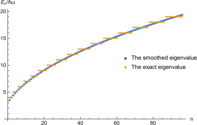
Figure 1: Comparison of the smoothed eigenvalue and the exact eigenvalue of a two bosonic oscillator system.

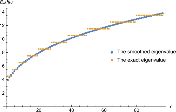
Figure 2: Comparison of the smoothed eigenvalue and the exact eigenvalue of a three bosonic oscillator system.

4 Noninteracting identical particles in a box: exchange energies

A quantum many-body system consisting of noninteracting identical particles corresponds to an ideal quantum gas.

There exist exchange interactions among identical particles. The influence of the quantum exchange interaction will be reflected in the eigenvalue, appearing as the exchange energy.

The method provides an approach to calculate the exchange energy with the help of statistical mechanics. In statistical mechanics, the contribution of exchange energies is taken into account by simply setting the maximum occupation number. That is, the information of exchange interactions of identical particles is embodied in the partition function of the system.

The canonical partition function of an $N$-particle quantum ideal gas is [31]

$$Z\left(\beta\right)\simeq\frac{1}{N!}z\left(\beta\right)^{N}\pm\frac{1}{2\left(N-2\right)!}z\left(\beta\right)^{N-2}z\left(2\beta\right)+\ldots,$$ (4.1)

where "$+$" stands for Bose gases, "$-$" stands for Fermi gases, and $z\left(\beta\right)$ is the single-particle partition function given by Eq. (3.2). Substituting Eq. (3.2) into Eq. (4.1) gives the canonical partition function of a quantum ideal gas,

$$Z\left(\beta\right)\simeq\frac{1}{N!}\left(\frac{V}{\lambda^{D}}\right)^{N}\pm\frac{1}{2^{1+D/2}\left(N-2\right)!}\left(\frac{V}{\lambda^{D}}\right)^{N-1}+\cdots.$$ (4.2)

The counting function is given by substituting Eq. (4.2) into Eq. (2.1):

$$N\left(E\right) \simeq\frac{1}{N!\Gamma\left(1+DN/2\right)}\left(\frac{V}{\Lambda^{D}}\right)^{N}E_{n}^{DN/2}$$

$$\pm\frac{1}{2^{1+D/2}\left(N-2\right)!\Gamma\left(1+D\left(N-1\right)/2\right)}\left(\frac{V}{\Lambda^{D}}\right)^{N-1}E_{n}^{DN/2-D/2}+\cdots,$$ (4.3)

where $\Lambda=\frac{h}{\sqrt{2\pi m}}$. Then solving Eq. (2.2) with the counting function (4.3) gives the eigenvalue,

$$E_{n} \simeq E_{n}^{cl}\left(N!\right)^{2/\left(DN\right)}\left[1+\right.$$

$$\left.\frac{2\left(1-N\right)}{D\left(1-N\right)^{2}\pm 2^{1+D/2}D\left(N!\right)^{1/N}\Gamma^{1/N-1}\left(1+DN/2\right)\Gamma\left(1+D\left(N-1\right)/2\right)n^{1/N}}\right],$$ (4.4)

where $E_{n}^{cl}$ is the eigenvalue of a system consisting of $N$ noninteracting particles given by Eq. (3.6). We make the assumption that the eigenvalue can be written in the form $E_{n}\sim\left(N!\right)^{2/\left(DN\right)}E_{n}^{cl}\left(1+\text{corrections}\right)$ with the corrections small enough. At higher excited states, i.e., the case of large $n$, this assumption is valid.

The influence of the quantum exchange interaction appears as the exchange energy in eigenvalues. From the result, Eq. (4.4), we can see the contribution of the exchange energy of bosons or fermions on the eigenvalue, partly reflected in the terms with the sign "$\pm$".

In order to illustrate the quantum exchange interaction, we consider a $D$-dimensional system consisting of two bosons or two fermions. By Eq. (4.4), the eigenvalue of such a two-particle system reads

$$\left.E_{n}\right|_{N=2}\simeq\left.E_{n}^{cl}\right|_{N=2}\left(2!\right)^{1/D}\left[1-\frac{2\sqrt{D!}}{D\sqrt{D!}\pm 2^{1+\left(D+1\right)/2}D\Gamma\left(1+D/2\right)n^{1/2}}\right],$$ (4.5)

where

$$\left.E_{n}^{cl}\right|_{N=2}=\frac{h^{2}}{2\pi mV^{2/D}}\Gamma^{1/D}\left(D+1\right)n^{1/D}$$ (4.6)

is the eigenvalue of classical particles.

For one-dimensional cases, the eigenvalue

$$\left.E_{n}\right|_{N=2}^{D=1}\simeq\frac{h^{2}}{\pi mL^{2}}\left(1-\frac{1}{1/2\pm\sqrt{\pi}n^{1/2}}\right)n,$$ (4.7)

for two-dimensional cases, the eigenvalue

$$\left.E_{n}\right|_{N=2}^{D=2}\simeq\frac{h^{2}}{\pi m\Omega}\left(1-\frac{1}{1\pm 4n^{1/2}}\right)n^{1/2},$$ (4.8)

and for three-dimensional cases, the eigenvalue

$$\left.E_{n}\right|_{N=2}^{D=3}\simeq\left(\frac{3}{2}\right)^{1/3}\frac{h^{2}}{\pi mV^{2/3}}\left(1-\frac{2/3}{1\pm\sqrt{6}\sqrt{\pi}n^{1/2}}\right)n^{1/3},$$ (4.9)

where $L$ is the length, $\Omega$ is the area, and $V$ is the volume of the container.

From Eq. (4.7) one can see that the quantum exchange interaction between bosons is attract and the quantum exchange interaction between fermions is repulsive.

5 Noninteracting identical particles in external fields

In this section, we calculate the eigenvalue of identical particles in an external field with the help of statistical mechanics.

For an ideal gas in an external field, the single-particle eigenvalue is determined by the Hamiltonian $H=-\frac{\hbar^{2}}{2m}\nabla^{2}+U\left(x\right)$. The partition function for a classical gas can be expressed as [2, 35, 1]

$$z\left(\beta\right)=\frac{V}{\lambda^{D}}\left(1+\sum_{k=1/2,1,\ldots}B_{k}\beta^{k}\right),$$ (5.1)

where $B_{k}$ is the heat kernel coefficient, e.g., $B_{1/2}=\frac{1}{V}\int dxU\left(x\right)$. Eq. (5.1) is known as the heat kernel expansion [1].

For quantum ideal gases in an external field, there are also quantum exchange interactions. In order to illustrate the influence of the quantum exchange interaction, we consider a $D$-dimensional system consisting of two bosons or two fermions. For the two-particle case, the exact canonical partition function is [31]

$$Z\left(\beta\right)=\frac{1}{2}z^{2}\left(\beta\right)\pm\frac{1}{2}z\left(2\beta\right).$$ (5.2)

Substituting Eq. (5.1) into Eq. (5.2) gives the canonical partition function:

$$Z\left(\beta\right)\simeq\frac{1}{2}\left(\frac{V}{\lambda^{D}}\right)^{2}+\left(\frac{V}{\lambda^{D}}\right)^{2}\sqrt{\beta}B_{1/2}\pm\frac{1}{2^{1+D/2}}\frac{V}{\lambda^{D}}+\ldots,$$ (5.3)

where the second term is the contribution of the external field, the third term is the contribution of the quantum exchange interaction.

The counting function can be obtained by substituting Eq. (5.3) into Eq. (2.1):

$$N\left(E\right) \simeq\frac{1}{2\Gamma\left(1+D\right)}\left(\frac{V}{\Lambda^{D}}\right)^{2}E^{D}+\frac{1}{\Gamma\left(1/2+D\right)}\left(\frac{V}{\Lambda^{D}}\right)^{2}B_{1/2}E^{D-1/2}$$

$$\pm\frac{1}{2^{1+D/2}\Gamma\left(1+D/2\right)}\frac{V}{\Lambda^{D}}E^{D/2}+\ldots.$$ (5.4)

Solving Eq (2.2) with the counting function Eq. (5.4) gives

$$\left.E_{n}\right|_{N=2}\simeq E_{n}^{cl}\left(N!\right)^{2/\left(ND\right)}\left[1-\frac{\pm 2c_{1}n^{1/\left(2D\right)-1/2}+2\left(B_{1/2}\Lambda V^{-1/D}\right)}{c_{2}n^{1/\left(2D\right)}\pm Dc_{1}n^{1/\left(2D\right)-1/2}+\left(2D-1\right)\left(B_{1/2}\Lambda V^{-1/D}\right)}\right],$$ (5.5)

where $c_{1}=2^{-3/2+1/\left(2D\right)-D/2}\left(D!\right)^{-1/2+1/\left(2D\right)}\frac{\Gamma\left(1/2+D\right)}{\Gamma\left(1+D/2\right)}$ and $c_{2}=2^{1/\left(2D\right)}D\left(D!\right)^{-1+1/\left(2D\right)}\Gamma\left(1/2+D\right)$.

From Eq. (5.5), one can see the influence of the external field, $B_{1/2}\Lambda V^{-1/D}$, and the influence of the quantum exchange interaction, partly reflected in the terms with the sign "$\pm$", on the eigenvalue of a quantum ideal gas.

For one-dimensional cases, the eigenvalue

$$\left.E_{n}\right|_{N=2}^{D=1}\simeq\frac{h^{2}}{\pi mL^{2}}\left[1-\frac{8\left(B_{1/2}\Lambda V^{-1/D}\right)\pm 2\sqrt{2}}{2\sqrt{2\pi}n^{1/2}+4\left(B_{1/2}\Lambda V^{-1/D}\right)\pm\sqrt{2}}\right]n,$$ (5.6)

for two-dimensional cases, the eigenvalue

$$\left.E_{n}\right|_{N=2}^{D=2}\simeq\frac{h^{2}}{\pi m\Omega}\left[1-\frac{32\left(B_{1/2}\Lambda V^{-1/D}\right)n^{1/4}\pm 3\sqrt{2\pi}}{12\sqrt{2\pi}n^{1/2}+48\left(B_{1/2}\Lambda V^{-1/D}\right)n^{1/4}\pm 3\sqrt{2\pi}}\right]n^{1/2},$$ (5.7)

and for three-dimensional cases, the eigenvalue

$$\left.E_{n}\right|_{N=2}^{D=3} \simeq\left(\frac{3}{2}\right)^{1/3}\frac{h^{2}}{\pi mV^{2/3}}\left[1\right.$$

$$\left.-\frac{192\left(B_{1/2}\Lambda V^{-1/D}\right)n^{1/3}\pm 10\times 2^{5/6}\times 3^{2/3}}{90\times 2^{1/3}\times 3^{1/6}\sqrt{\pi}n^{1/2}+480\left(B_{1/2}\Lambda V^{-1/D}\right)n^{1/3}\pm 15\times 2^{5/6}\times 3^{2/3}}\right]n^{1/3}.$$ (5.8)

6 Influences of topologies on eigenvalues

In this section, we discuss the topology effect on the eigenvalue of classical and quantum particles in nontrivial topological containers. Classical and quantum particles in quantum mechanics corresponds to classical and quantum gases in statistical mechanics. In statistical mechanics, the geometric effect and the topology effect are systematically studied [36, 37, 38, 39, 40, 41]. In the following, we calculate the eigenvalue from the result given by statistical mechanics.

6.1 Non-interacting classical particles in a two-dimensional nontrivial topological box

The single-particle partition function of a two-dimensional ideal classical gas in a nontrivial topological box is indeed the global heat kernel given by Kac in his famous paper "Can one hear the shape of a drum?" [13]. Kac’s result allows us to discuss the influence of topology of space on the eigenvalue.

The single-particle partition function of a two-dimensional confined ideal classical gas is just the global heat kernel given by Kac [13]

$$z\left(\beta\right)=\frac{\Omega}{\lambda^{2}}-\frac{1}{4}\frac{L}{\lambda}+\frac{\chi}{6},$$ (6.1)

where $\Omega$ is the area and $L$ the perimeter of the two-dimensional container. $\chi=1-r$ here is the Euler-Poincaré characteristic number with $r$ the number of holes in the two-dimensional container, which describes the connectivity, a topological property of the system.

First consider the eigenvalue of a particle in a nontrivial topological box. From Eq. (2.1), we can obtain the counting function,

$$N\left(E\right)=\frac{\Omega}{\Lambda^{2}}E-\frac{1}{2\sqrt{\pi}}\frac{L}{\Lambda}E^{1/2}+\frac{\chi}{6}.$$ (6.2)

Solving Eq. (2.2) with the counting function Eq. (6.2) gives the eigenvalue

$$E_{n} =\frac{h^{2}}{2\pi m\Omega}\left[n+\frac{1}{2\pi}\left(\frac{L}{\sqrt{\Omega}}\right)\sqrt{n\pi+\frac{1}{16}\left(\frac{L}{\sqrt{\Omega}}\right)^{2}-\frac{\pi}{6}\chi}\right.$$

$$\left.+\frac{1}{8\pi}\left(\frac{L}{\sqrt{\Omega}}\right)^{2}-\frac{1}{6}\chi\right].$$ (6.3)

From the expression of the eigenvalue, Eq. (6.3), we can see the geometric effect, reflected in the terms with the factor $\frac{L}{\sqrt{\Omega}}$, and the topological effect, reflected in the terms with the factor $\chi$, explicitly.

6.2 Non-interacting quantum particles in a two-dimensional nontrivial topological box

For two-particle ideal quantum systems, the canonical partition function can be obtained by substituting Eq. (6.1) into Eq. (5.2):

$$Z\left(\beta\right)\simeq\frac{1}{2}\left(\frac{\Omega}{\lambda^{2}}\right)^{2}-\frac{1}{4}\frac{L}{\lambda}\frac{\Omega}{\lambda^{2}}\pm\frac{1}{2}\frac{\Omega}{\lambda^{2}}+\frac{1}{32}\left(\frac{L}{\lambda}\right)^{2}+\frac{\chi}{6}\frac{\Omega}{\lambda^{2}}+\ldots.$$ (6.4)

The counting function is given by substituting Eq. (6.4) into Eq. (2.1):

$$N\left(E\right) \simeq\frac{1}{4}\left(\frac{\Omega}{\Lambda^{2}}\right)^{2}E^{2}-\frac{1}{3\sqrt{\pi}}\frac{L}{\Lambda}\frac{\Omega}{\Lambda^{2}}E^{3/2}\pm\frac{1}{2}\frac{\Omega}{\Lambda^{2}}E$$

$$+\frac{1}{32}\left(\frac{L}{\Lambda}\right)^{2}E+\frac{\chi}{6}\frac{\Omega}{\Lambda^{2}}E+\ldots.$$ (6.5)

Solving Eq. (2.2) with the counting function Eq. (6.5) gives the eigenvalue

$$\left.E_{n}\right|_{N=2}\simeq\frac{h^{2}}{\pi m\Omega}\left[1-\frac{-\frac{2\sqrt{2}}{3}\frac{L}{\sqrt{\Omega}}n^{3/4}+\sqrt{\pi}\left(\pm 1+\frac{1}{3}\chi+\frac{1}{16}\frac{L^{2}}{\Omega}\right)n^{1/2}}{2\sqrt{\pi}n-\sqrt{2}\frac{L}{\sqrt{\Omega}}n^{3/4}+\sqrt{\pi}\left(\pm 1+\frac{1}{3}\chi+\frac{1}{16}\frac{L^{2}}{\Omega}\right)n^{1/2}}\right]n^{1/2}.$$ (6.6)

From Eq. (6.6), one can see that the eigenvalue of a two-dimensional ideal quantum gas in a nontrivial topological box is modified by the geometric effect described by $\frac{L}{\sqrt{\Omega}}$, and by the topological effect described by $\chi$. Moreover, for such quantum cases, there exist exchange energies partly reflected in the terms with the sign "$\pm$".

7 Interacting classical many-body systems with the Lennard-Jones interaction

A system consisting of particles interacted with each other through the Lennard-Jones potential in quantum mechanics corresponds to an interacting gas with the Lennard-Jones interaction in statistical mechanics.

The Lennard-Jones inter-particle potential reads

$$U=4\varepsilon\left[\left(\frac{\sigma}{r}\right)^{12}-\left(\frac{\sigma}{r}\right)^{6}\right],$$ (7.1)

where $\varepsilon$ is the depth of the potential well and $\sigma$ is the finite distance at which the inter-particle potential is zero [42]. The canonical partition function of a classical interacting gas with $N$ particles is given by [31]

$$Z\left(\beta\right)\simeq\frac{1}{N!}\left(\frac{V}{\lambda^{3}}\right)^{N}+\frac{1}{\left(N-2\right)!}\left(\frac{V}{\lambda^{3}}\right)^{N-1}b_{2}+\ldots,$$ (7.2)

where $b_{2}=\frac{2\pi}{\lambda^{3}}\int d^{3}r\left(e^{-\beta U}-1\right)$.

The coefficient $b_{2}$ for the Lennard-Jones interaction is [42]

$$b_{2}\simeq\frac{2\pi}{3}\frac{r_{0}^{3}}{\lambda^{3}}\left(u_{0}\beta-1\right),$$ (7.3)

where $r_{0}=2^{1/6}\sigma$. Then the canonical partition reads

$$Z\left(\beta\right)\simeq\frac{1}{N!}\left(\frac{V}{\lambda^{3}}\right)^{N}-\frac{2\pi}{3\left(N-2\right)!}\left(\frac{V}{\lambda^{3}}\right)^{N}\frac{r_{0}^{3}}{V}+\frac{2\pi}{3\left(N-2\right)!}\left(\frac{V}{\lambda^{3}}\right)^{N}\frac{r_{0}^{3}}{V}u_{0}\beta+\ldots.$$ (7.4)

The counting function can be obtained by substituting Eq. (7.4) into Eq. (2.1),

$$N\left(E\right) \simeq\frac{1}{N!\Gamma\left(1+3N/2\right)}\left(\frac{V}{\Lambda^{3}}\right)^{N}E^{3N/2}-\frac{2\pi}{3\left(N-2\right)!\Gamma\left(1+3N/2\right)}\frac{r_{0}^{3}}{V}\left(\frac{V}{\Lambda^{3}}\right)^{N}E^{3N/2}$$

$$+\frac{2\pi}{3\left(N-2\right)!\Gamma\left(3N/2\right)}\frac{r_{0}^{3}}{V}u_{0}\left(\frac{V}{\Lambda^{3}}\right)^{N}E^{3N/2-1}+\ldots.$$ (7.5)

The eigenvalue can be obtained by solving Eq. (2.2) with the counting function (7.5):

$$E_{n} \simeq E_{n}^{cl}\left(N!\right)^{2/\left(3N\right)}\left[1\right.$$

$$\left.+\frac{4\left(N!\right)^{2/\left(3N\right)}\Gamma^{2/\left(3N\right)}\left(1+3N/2\right)r_{0}^{3}n^{2/\left(3N\right)}-6Nr_{0}^{3}V^{2/3}u_{0}\Lambda^{-2}}{3\left(N!\right)^{2/\left(3N\right)}\Gamma^{2/\left(3N\right)}\left(1+3N/2\right)\left[\frac{3}{\left(N-1\right)\pi}V-2Nr_{0}^{3}\right]n^{2/\left(3N\right)}+3N\left(3N-2\right)r_{0}^{3}V^{2/3}u_{0}\Lambda^{-2}}\right].$$ (7.6)

Especially, for $N=1$, there is of course no inter-particle interactions, so the eigenvalue (7.6) recovers the eigenvalue of a free particle

$$\left.E_{n}\right|_{N=1}\simeq\frac{3^{2/3}}{2^{7/3}}\frac{h^{2}}{m\pi^{2/3}V^{2/3}}n^{2/3}.$$ (7.7)

For $N=2$, the eigenvalue (7.6) becomes

$$\left.E_{n}\right|_{N=2}\simeq\left(\frac{3}{2}\right)^{1/3}\frac{h^{2}}{\pi mV^{2/3}}\left[1+\frac{12^{1/3}\times\frac{4}{3}\pi r_{0}^{3}n^{1/3}-4\pi r_{0}^{3}V^{2/3}u_{0}\Lambda^{-2}}{3\times 12^{1/3}\left(V-\frac{4}{3}\pi r_{0}^{3}\right)n^{1/3}+8\pi r_{0}^{3}V^{2/3}u_{0}\Lambda^{-2}}\right]n^{1/3}.$$ (7.8)

8 Interacting quantum many-body systems with hard-sphere interactions

A system consisting of particles interacted with each other through the hard-sphere potential in quantum mechanics corresponds to an interacting gas with the hard-sphere interaction in statistical mechanics.

In a quantum hard-sphere gas, there exist both the quantum exchange interaction and the classical hard-sphere interaction. The canonical partition function of a quantum interacting gas is [31]

$$Z\left(\beta\right)\simeq\frac{1}{N!}\left(\frac{V}{\lambda^{3}}\right)^{N}+\frac{1}{\left(N-2\right)!}\left(\frac{V}{\lambda^{3}}\right)^{N-1}b_{2}+\ldots,$$ (8.1)

where

$$b_{2}=\frac{1}{2V\lambda^{3}}\int d^{6}qU_{2}\left(q_{1},q_{2}\right)$$ (8.2)

with $U_{2}\left(q_{1},q_{2}\right)=\lambda^{6}\left[\langle q_{1},q_{2}|e^{-\beta H_{2}}|q_{1},q_{2}\rangle-\langle q_{1}|e^{-\beta H_{1}}|q_{1}\rangle\langle q_{2}|e^{-\beta H_{1}}|q_{2}\rangle\right]$, $H_{1}=-\frac{\hbar^{2}}{2m}\nabla^{2}$, $H_{2}=-\frac{\hbar^{2}}{2m}\nabla_{1}^{2}-\frac{\hbar^{2}}{2m}\nabla_{2}^{2}+4\pi a\hbar^{2}/m\delta\left(q_{1}-q_{2}\right)$, and $a$ is the radius of the particle.

For Bose gases, Eq. (8.2) becomes $b_{2}=2^{-5/2}-2\frac{a}{\lambda}-\frac{10\pi^{2}}{3}\frac{a^{5}}{\lambda^{5}}$ [42]; for Fermi gases, Eq. (8.2) becomes $b_{2}=-2^{-5/2}-6\pi\frac{a^{3}}{\lambda^{3}}+18\pi^{2}\frac{a^{5}}{\lambda^{5}}$ [42].

Then the canonical partition function of a Bose gas is

$$Z_{B}\left(\beta\right)\simeq\frac{1}{N!}\left(\frac{V}{\lambda^{3}}\right)^{N}+\frac{1}{\left(N-2\right)!}\left(\frac{V}{\lambda^{3}}\right)^{N-1}\left(2^{-5/2}-2\frac{a}{\lambda}-\frac{10\pi^{2}}{3}\frac{a^{5}}{\lambda^{5}}\right)+\ldots,$$ (8.3)

and the canonical partition function of a Fermi gas is

$$Z_{F}\left(\beta\right)\simeq\frac{1}{N!}\left(\frac{V}{\lambda^{3}}\right)^{N}+\frac{1}{\left(N-2\right)!}\left(\frac{V}{\lambda^{3}}\right)^{N-1}\left(-2^{-5/2}-6\pi\frac{a^{3}}{\lambda^{3}}+18\pi^{2}\frac{a^{5}}{\lambda^{5}}\right)+\ldots,$$ (8.4)

respectively.

Then the counting function of a Bose gas by Eq. (2.1) is

$$N_{B}\left(E\right)$$

$$\simeq\frac{\left(2\pi\right)^{3N/2}}{N!\Gamma\left(1+3N/2\right)}\frac{m^{3N/2}V^{N}}{h^{3N}}E^{3N/2}+\frac{2^{3N/2-4}\pi^{3\left(N-1\right)/2}}{\left(N-2\right)!\Gamma\left(3N/2-1/2\right)}\frac{m^{3\left(N-1\right)/2}V^{N-1}}{h^{3\left(N-1\right)}}E^{3N/2-3/2}$$ (8.5)

$$-\frac{2^{3N/2}\pi^{\left(3N-2\right)/2}a}{\left(N-2\right)!\Gamma\left(3N/2\right)}\frac{m^{\left(3N-2\right)/2}V^{N-1}}{h^{3N-2}}E^{3N/2-1}-\frac{10a^{5}\left(2\pi\right)^{3N/2+3}}{3\left(N-2\right)!\Gamma\left(3N/2+2\right)}\frac{m^{\left(3N+2\right)/2}V^{N-1}}{h^{3N+2}}E^{3N/2+1}+\ldots,$$ (8.6)

and the counting function of a Fermi gas by Eq. (2.1) is

$$N_{F}\left(E\right)$$

$$\simeq\frac{\left(2\pi\right)^{3N/2}}{N!\Gamma\left(1+3N/2\right)}\frac{m^{3N/2}V^{N}}{h^{3N}}E^{3N/2}-\frac{2^{3N/2-4}\pi^{3N/2-3/2}}{\left(N-2\right)!\Gamma\left(3N/2-1/2\right)}\frac{m^{3N/2-\frac{3}{2}V^{N-1}}}{h^{3N-3}}E^{3N/2-3/2}$$ (8.7)

$$-\frac{3\times 2^{3N/2+1}\pi^{3N/2+1}a^{3}}{\left(N-2\right)!\Gamma\left(3N/2+1\right)}\frac{m^{3N/2}V^{N-1}}{h^{3N}}E^{3N/2}+\frac{9\times 2^{3N/2+2}\pi^{3N/2+3}a^{5}}{\left(N-2\right)!\Gamma\left(3N/2+2\right)}\frac{m^{3N/2+1}V^{N-1}}{h^{3N+2}}E^{3N/2+1}+\ldots.$$ (8.8)

Solving Eq. (2.2) gives the eigenvalue of a hard-sphere Bose gas,

$$E_{n}\simeq E_{n}^{cl}\left(N!\right)^{2/3N}\left[1+\frac{h_{1}\frac{a^{5}}{V^{5/3}}n^{5/\left(3N\right)}+2h_{2}\frac{a}{V^{1/3}}n^{1/\left(3N\right)}-2h_{3}}{h_{1}\frac{a^{5}}{V^{5/3}}n^{5/\left(3N\right)}+h_{4}n^{1/N}+5h_{2}\frac{a}{V^{1/3}}n^{1/\left(3N\right)}+3\left(N-1\right)h_{3}}\right]$$ (8.9)

with $h_{1}=\frac{10\pi^{2}\left(N!\right)^{5/\left(3N\right)}\Gamma^{5/\left(3N\right)}\left(1+3N/2\right)}{3\Gamma\left(3N/2+2\right)}$, $h_{2}=\frac{2\left(N!\right)^{1/\left(3N\right)}\Gamma^{1/\left(3N\right)}\left(1+3N/2\right)}{\Gamma\left(3N/2\right)}$, $h_{3}=\frac{1}{2^{5/2}\Gamma\left(3N/2-1/2\right)}$, and $h_{4}=\frac{3\left(N!\right)^{1/N}\Gamma^{1/N-1}\left(1+3N/2\right)}{N-1}$. The eigenvalue of a hard-sphere Fermi gas,

$$E_{n}\simeq E_{n}^{cl}\left(N!\right)^{2/\left(3N\right)}\left[1+\frac{-2t_{1}\frac{a^{5}}{V^{5/3}}n^{5/\left(3N\right)}+2t_{2}\frac{a^{3}}{V}n^{1/N}+2t_{3}}{\left(2+3N\right)t_{1}\frac{a^{5}}{V^{5/3}}n^{5/\left(3N\right)}+t_{4}n^{1/N}-3Nt_{2}\frac{a^{3}}{V}n^{1/N}-3\left(N-1\right)t_{3}}\right]$$ (8.10)

with $t_{1}=\frac{18\pi^{2}\left(N!\right)^{5/\left(3N\right)}\Gamma^{5/\left(3N\right)}\left(1+3N/2\right)}{\Gamma\left(3N/2+2\right)}$, $t_{2}=\frac{6\pi\left(N!\right)^{1/\left(3N\right)}\Gamma^{1/\left(3N\right)}\left(1+3N/2\right)}{\Gamma\left(3N/2+1\right)}$, $t_{3}=\frac{1}{2^{5/2}\Gamma\left(3N/2-1/2\right)}$, and $t_{4}=3\frac{\left(N!\right)^{1/N}\Gamma^{1/N-1}\left(1+3N/2\right)}{N-1}$.

In order to illustrate the influence of the quantum exchange interaction, we consider a system consisting of two bosons or two fermions. For the Bose case, the eigenvalue (4.5) becomes

$$\left.E_{n}\right|_{N=2}^{Bose}\overset{D=3}{\sim}12^{1/3}\frac{h^{2}}{2\pi mV^{2/3}}n^{1/3}\left[1\right.$$

$$\left.+\frac{10\times 2^{1/3}\times 3^{5/6}\pi^{5/2}\frac{a^{5}}{V^{5/3}}n^{5/6}+36\times 3^{1/6}\sqrt{\pi}\frac{a}{V^{1/3}}n^{1/6}-6\times 2^{1/6}}{-40\times 2^{1/3}\times 3^{5/6}\pi^{5/2}\frac{a^{5}}{V^{5/3}}n^{5/6}-72\times 3^{1/6}\sqrt{\pi}\frac{a}{V^{1/3}}n^{1/6}+9\times 2^{1/6}\sqrt{6\pi}\sqrt{n}+9\times 2^{1/6}}\right];$$ (8.11)

for the Fermi case, the eigenvalue (4.5) becomes

$$\left.E_{n}\right|_{N=2}^{Fermi}\overset{D=3}{\sim}12^{1/3}\frac{h^{2}}{2\pi mV^{2/3}}n^{1/3}\left[1\right.$$ (8.12)

$$\left.+\frac{-18\times 2^{2/3}\times 3^{5/6}\pi^{5/2}\frac{a^{5}}{V^{5/3}}n^{5/6}+24\sqrt{3}\pi^{3/2}\frac{a^{3}}{V}\sqrt{n}+2\sqrt{2}}{72\times 2^{2/3}\times 3^{5/6}\pi^{5/2}\frac{a^{5}}{V^{5/3}}n^{5/6}-72\sqrt{3}\pi^{3/2}\times\frac{a^{3}}{V}\sqrt{n}+6\sqrt{3\pi}\sqrt{n}-3\sqrt{2}}\right].$$ (8.13)

9 The one-dimensional Ising model

The eigenvalue of the one-dimensional Ising model without interactions can be calculated from the corresponding canonical partition function directly.

9.1 The Ising model without interactions

For a one-dimensional $N$-particle Ising model without the interaction between spins, the canonical partition function reads [33]

$$Z(\beta)=(e^{\beta B\mu}+e^{-B\mu\beta})^{N},$$ (9.1)

where $B$ is the magnetic field strength and $\mu$ is the spin magnetic moment.

The counting function can be obtained by substituting Eq. (9.1) into Eq. (2.1),

$$N(E)=\sum_{s=1}^{N+1}\binom{N}{s-1}\theta\left(E-B\mu\left[2\left(s-1\right)-N\right]\right),$$ (9.2)

where $\theta\left(x\right)$ is the step function. Substituting Eq. (9.2) into Eq. (2.2) and solving the equation give the eigenvalue

$$E=B\mu\left[2\left(n-1\right)-N\right]$$ (9.3)

and the degree of degeneracy

$$\omega(E)=\binom{N}{n-1}.$$ (9.4)

9.2 The Ising model with nearest-neighbour interactions

For a one-dimensional $N$-particle Ising model with nearest-neighbour interactions, the Hamiltonian is $H=-\sum_{i}B\mu\sigma_{i}+\sum_{i}\epsilon\sigma_{i}\sigma_{i+1}$, where $\epsilon$ is the coupling constant. The canonical partition function reads [43]

$$Z\left(\beta,N\right)=\lambda_{+}^{N}+\lambda_{-}^{N},$$ (9.5)

where

$$\lambda_{\pm}=e^{\beta\epsilon}\left[\cosh\left(\beta\mu B\right)\pm\sqrt{\cosh^{2}\left(\beta\mu B\right)-2e^{-2\beta\epsilon}\sinh\left(2\beta\epsilon\right)}\right].$$ (9.6)

The counting function can be obtained by substituting Eq. (9.5) into Eq. (2.1). In the following, we list the eigenvalues for $N=3,4,5,\ldots,9$.

For example, for $N=3$, the counting function is

$$N\left(E\right) =\theta\left(E-\left(-3B\mu-3\epsilon\right)\right)+3\theta\left(E-\left(-B\mu+\epsilon\right)\right)$$

$$+3\theta\left(E-\left(B\mu+\epsilon\right)\right)+\theta\left(E-\left(3B\mu-3\epsilon\right)\right);$$ (9.7)

the eigenvalue $E$ and the degree of degeneracy $\omega$ are listed in Table 1.

Table 1: The eigenvalue $E$ and the degree of degeneracy $\omega$ : $N=3$

$E$	$-3B\mu-3\epsilon$	$-B\mu+\epsilon$	$B\mu+\epsilon$	$3B\mu-3\epsilon$
$\omega$	$1$	$3$	$3$	$1$

For other values of $N$, we only list the eigenvalues in Tables 2-7.

Table 2: The eigenvalue $E$ and the degree of degeneracy $\omega$ : $N=4$

$E$	$-4B\mu-4\epsilon$	$-2B\mu$	$0$	$4\epsilon$	$2B\mu$	$4B\mu-4\epsilon$
$\omega$	$1$	$4$	$4$	$2$	$4$	$1$

Table 3: The eigenvalue $E$ and the degree of degeneracy $\omega$ : $N=5$

$E$	$-5B\mu-5\epsilon$	$-3B\mu-\epsilon$	$-B\mu+3\epsilon$	$-B\mu-\epsilon$	$B\mu+3\epsilon$
$\omega$	$1$	$5$	$5$	$5$	$5$
$E$	$B\mu-\epsilon$	$3B\mu-\epsilon$	$5B\mu-5\epsilon$
$\omega$	$5$	$5$	$1$

Table 4: The eigenvalue $E$ and the degree of degeneracy $\omega$ : $N=6$

$E$	$-6B\mu-6\epsilon$	$-4B\mu-2\epsilon$	$-2B\mu+2\epsilon$	$-2B\mu-2\epsilon$	$-2\epsilon$
$\omega$	$1$	$6$	$9$	$6$	$6$
$E$	$2\epsilon$	$6\epsilon$	$2B\mu+2\epsilon$	$2B\mu-2\epsilon$	$4B\mu-2\epsilon$	$6B\mu-6\epsilon$
$\omega$	$12$	$2$	$9$	$6$	$6$	$1$

Table 5: The eigenvalue $E$ and the degree of degeneracy $\omega$ : $N=7$

$E$	$-7B\mu-7\epsilon$	$-5B\mu-3\epsilon$	$-3B\mu+\epsilon$	$-3B\mu-3\epsilon$	$-B\mu+5\epsilon$	$-B\mu+\epsilon$
$\omega$	$1$	$7$	$14$	$7$	$7$	$21$
$E$	$-B\mu-3\epsilon$	$B\mu+5\epsilon$	$B\mu+\epsilon$	$B\mu-3\epsilon$	$3B\mu+\epsilon$	$3B\mu-3\epsilon$
$\omega$	$7$	$7$	$21$	$7$	$14$	$7$
$E$	$5B\mu-3\epsilon$	$7B\mu-7\epsilon$
$\omega$	$7$	$1$

Table 6: The eigenvalue $E$ and the degree of degeneracy $\omega$ : $N=8$

$E$	$-8B\mu-8\epsilon$	$-6B\mu-4\epsilon$	$-4B\mu$	$-4B\mu-4\epsilon$	$-2B\mu+4\epsilon$	$-2B\mu$
$\omega$	$1$	$8$	$20$	$8$	$16$	$32$
$E$	$-2B\mu-4\epsilon$	$8\epsilon$	$-4\epsilon$	$0$	$4\epsilon$	$2B\mu$
$\omega$	$8$	$2$	$8$	$36$	$24$	$32$
$E$	$2B\mu+4\epsilon$	$2B\mu-4\epsilon$	$4B\mu-4\epsilon$	$4B\mu$	$6B\mu-4\epsilon$	$8B\mu-8\epsilon$
$\omega$	$16$	$8$	$8$	$20$	$8$	$1$

Table 7: The eigenvalue $E$ and the degree of degeneracy $\omega$ : $N=9$

$E$	$-9B\mu-9\epsilon$	$-7B\mu-5\epsilon$	$-5B\mu-5\epsilon$	$-5B\mu-\epsilon$	$-3B\mu-5\epsilon$	$-3B\mu-\epsilon$
$\omega$	$1$	$9$	$9$	$27$	$9$	$45$
$E$	$-3B\mu+3\epsilon$	$-B\mu-5\epsilon$	$-B\mu-\epsilon$	$-B\mu+3\epsilon$	$-B\mu+7\epsilon$	$B\mu-5\epsilon$
$\omega$	$30$	$9$	$54$	$54$	$9$	$9$
$E$	$B\mu-\epsilon$	$B\mu+3\epsilon$	$B\mu+7\epsilon$	$3B\mu-5\epsilon$	$3B\mu-\epsilon$	$3B\mu+3\epsilon$
$\omega$	$54$	$54$	$9$	$9$	$45$	$30$
$E$	$5B\mu-\epsilon$	$5B\mu-5\epsilon$	$7B\mu-5\epsilon$	$9B\mu-9\epsilon$
$\omega$	$27$	$9$	$9$	$1$

10 The one-dimensional Potts model

The Potts model in statistical mechanics is a generalization of the Ising model, which is a model of interacting spins on a crystalline lattice. The Hamiltonian of the one-dimensional Potts model is $H=-J\sum_{\left\langle i,j\right\rangle}\delta\left(\sigma_{i},\sigma_{j}\right)$, where $\sigma_{i}=1,2,3,\ldots,q$, $\delta\left(\sigma_{i},\sigma_{j}\right)=1$ if $i=j$, and $\left(\sigma_{i},\sigma_{j}\right)=0$ other wise. The canonical partition function of the one-dimensional Potts model of $N$ particles is [44]

$$Z\left(\beta,N\right)=q\left(q-1+e^{\beta J}\right)^{N-1}.$$ (10.1)

The counting function can be obtained by substituting Eq. (10.1) into Eq. (2.1),

$$N\left(E\right)=q\sum_{l=0}^{N-1}\binom{N-1}{l}\left(q-1\right)^{N-1-l}\theta\left(Jl+E\right).$$ (10.2)

Substituting Eq. (10.2) into Eq. (2.2) and solving the equation give the eigenvalue

$$E=nJ$$ (10.3)

and the degeneracy

$$\omega=q\binom{N-1}{n}\left(q-1\right)^{N-1-n}-q\binom{N-1}{n-1}\left(q-1\right)^{N-n}.$$ (10.4)

11 Conclusions

In this paper, we suggest a method for calculating the eigenvalue of a many-body system from the corresponding canonical partition function. The advantage of the method is that it allows us to merely calculate the eigenvalue without solving the eigenfunction simultaneously. Recalling that in many approximate methods, although only needing the eigenvalue, one has to solve the eigenfunction in the meantime. Solving eigenfunctions, however, is always a difficult task.

In statistical mechanics, the calculation of thermodynamic quantities only needs the knowledge of eigenvalues. Only the information of eigenvalue is embodied in thermodynamic quantities. The method suggested in the present paper is an approach for extracting the eigenvalue from the thermodynamic quantity which obtained by statistical mechanical method.

In the present paper, we calculate the eigenvalue from the canonical partition function. In future works, one can generalizes the method to calculate the eigenvalue from the other thermodynamic quantities.

Moreover, we improve the result of the relation between the counting function and the heat kernel given in [2].

Appendix A The relation between counting functions and heat kernels

In Ref. [2], we provide a relation between the counting function

$$N\left(\lambda\right)=\sum_{\lambda_{n}<\lambda}1$$ (A.1)

and the global heat kernel

$$K\left(t\right)=\sum_{n}e^{-\lambda_{n}t}.$$ (A.2)

In Ref. [2], we only consider the counting function which counts the number of eigenstates with eigenvalue smaller than a given number $\lambda$, but a special case is ignored: the given number is just a eigenvalue, i.e., $\lambda=\lambda_{n}$ with $\lambda_{n}$ the $n$-th eigenvalue. In the following, we provide a complete version of the relation between $N\left(\lambda\right)$ and $K\left(t\right)$.

Theorem 1

$$N\left(\lambda\right)= \frac{1}{2\pi i}\int_{c-i\infty}^{c+i\infty}K\left(t\right)\frac{e^{\lambda t}}{t}dt,\text{ when }\lambda_{n}\neq\lambda$$ (A.3)

$$N\left(\lambda\right)= \frac{1}{2\pi i}\int_{c-i\infty}^{c+i\infty}K\left(t\right)\frac{e^{\lambda t}}{t}dt-\frac{1}{2},\text{ when }\lambda_{n}=\lambda$$ (A.4)

with $c>\lim_{n\rightarrow\infty}\frac{\ln n}{\lambda_{n}}$.

Proof. The function

$$f\left(s\right)=\sum_{n=1}^{\infty}\frac{a_{n}}{\mu_{n}^{s}}$$ (A.5)

is a generalization of the Dirichlet series. The function

$$f\left(s+\omega\right)=\sum_{n=1}^{\infty}\frac{a_{n}}{\mu_{n}^{s+\omega}}$$ (A.6)

is uniformly convergent when $\sigma>\beta-c$, where $c=\operatorname{Re}\omega$ and $\beta$ is the abscissa of absolute convergence of this Dirichlet series. Performing the integral $\frac{1}{2\pi i}\int_{c-iT}^{c+iT}\frac{x^{\omega}}{\omega}d\omega$ on both sides of Eq. (A.6) gives

$$\frac{1}{2\pi i}\int_{c-iT}^{c+iT}f\left(s+\omega\right)\frac{x^{\omega}}{\omega}d\omega=\frac{1}{2\pi i}\sum_{n=1}^{\infty}\frac{a_{n}}{\mu_{n}^{s}}\int_{c-iT}^{c+iT}\left(\frac{x}{\mu_{n}}\right)^{\omega}\frac{d\omega}{\omega}.$$ (A.7)

The integral in the right-hand side of Eq. (A.7), $\frac{1}{2\pi i}\int_{c-iT}^{c+iT}\left(\frac{x}{\mu_{n}}\right)^{\omega}\frac{d\omega}{\omega}$, should be considered in different situations, i.e., $\mu_{n}<x$, $\mu_{n}=x$, and $\mu_{n}>x$. In the limitation $T\rightarrow\infty$, the integral reads [45]

$$\lim_{T\rightarrow\infty}\frac{1}{2\pi i}\int_{c-iT}^{c+iT}\left(\frac{x}{\mu_{n}}\right)^{\omega}\frac{d\omega}{\omega}=\left\{\begin{array}[c]{c}\displaystyle 1,\text{ }\mu_{n}<x,\\ \displaystyle\frac{1}{2},\text{ }\mu_{n}=x,\\ \displaystyle 0,\text{ }\mu_{n}>x.\end{array}\right.$$ (A.8)

Substituting Eq. (A.8) into Eq. (A.7) gives

$$\frac{1}{2\pi i}\int_{c-i\infty}^{c+i\infty}f\left(s+\omega\right)\frac{x^{\omega}}{\omega}d\omega=\left\{\begin{array}[c]{c}\displaystyle\sum_{\mu_{n}<x}^{\infty}\frac{a_{n}}{\mu_{n}^{s}}\text{, when }\mu_{n}\neq x,\\ \displaystyle\sum_{\mu_{n}<x}^{\infty}\frac{a_{n}}{\mu_{n}^{s}}+\frac{1}{2}\frac{a_{n_{x}}}{x^{s}}\text{, when }\mu_{n}=x.\end{array}\right.$$ (A.9)

Setting $s=0$, $a_{n}=1$, $\mu_{n}=e^{\lambda_{n}}$, $x=e^{\lambda}$, and $\omega=t$ in Eq. (A.9) gives

$$\frac{1}{2\pi i}\int_{c-i\infty}^{c+i\infty}f\left(t\right)\frac{e^{\lambda t}}{t}d\omega=\left\{\begin{array}[c]{c}\displaystyle\sum_{\lambda_{n}<\lambda}^{\infty}1,\text{ when }\lambda_{n}\neq\lambda,\\ \displaystyle\sum_{\lambda_{n}<\lambda}^{\infty}1+\frac{1}{2},\text{ when }\lambda_{n}=\lambda.\end{array}\right.$$ (A.10)

Comparing the definition of the counting function and the global heat kernel, Eqs. (A.1) and (A.2), with Eq. (A.10) proves Eqs. (A.3) and (A.4).

References

• [1] D. V. Vassilevich, Heat kernel expansion: user’s manual, Physics reports 388 (2003), no. 5 279–360.
• [2] W.-S. Dai and M. Xie, The number of eigenstates: counting function and heat kernel, Journal of High Energy Physics 2009 (2009), no. 02 033.
• [3] W.-S. Dai and M. Xie, An approach for the calculation of one-loop effective actions, vacuum energies, and spectral counting functions, Journal of High Energy Physics 2010 (2010), no. 6 1–29.
• [4] W. Dai and M. Xie, Hard-sphere gases as ideal gases with multi-core boundaries: An approach to two-and three-dimensional interacting gases, EPL (Europhysics Letters) 72 (2005), no. 6 887.
• [5] G. Gentile j, itosservazioni sopra le statistiche intermedie, Il Nuovo Cimento (1924-1942) 17 (1940), no. 10 493–497.
• [6] A. Khare, Fractional statistics and quantum theory. World Scientific, 2005.
• [7] W.-S. Dai and M. Xie, Calculating statistical distributions from operator relations: The statistical distributions of various intermediate statistics, Annals of Physics 332 (2012) 166–179.
• [8] A. Algin and A. Olkun, Bose–einstein condensation in low dimensional systems with deformed bosons, Annals of Physics 383 (2017) 239–256.
• [9] W.-S. Dai and M. Xie, Intermediate-statistics spin waves, Journal of Statistical Mechanics: Theory and Experiment 2009 (2009), no. 04 P04021.
• [10] V. P. Maslov, The relationship between the fermi–dirac distribution and statistical distributions in languages, Mathematical Notes 101 (2017), no. 3-4 645–659.
• [11] W.-S. Dai and M. Xie, Gentile statistics with a large maximum occupation number, Annals of Physics 309 (2004), no. 2 295–305.
• [12] W.-S. Dai and M. Xie, An exactly solvable phase transition model: generalized statistics and generalized bose–einstein condensation, Journal of Statistical Mechanics: Theory and Experiment 2009 (2009), no. 07 P07034.
• [13] M. Kac, Can one hear the shape of a drum?, The american mathematical monthly 73 (1966), no. 4 1–23.
• [14] A. J. Maciejewski, M. Przybylska, and T. Stachowiak, Full spectrum of the rabi model, Physics Letters A 378 (2014), no. 1 16–20.
• [15] S. Faldella, N. Kitanine, and G. Niccoli, The complete spectrum and scalar products for the open spin-1/2 xxz quantum chains with non-diagonal boundary terms, Journal of Statistical Mechanics: Theory and Experiment 2014 (2014), no. 1 P01011.
• [16] G. Niccoli, Antiperiodic spin-1/2 xxz quantum chains by separation of variables: complete spectrum and form factors, Nuclear Physics B 870 (2013), no. 2 397–420.
• [17] M. Mierzejewski, T. Prosen, D. Crivelli, and P. Prelovšek, Eigenvalue statistics of reduced density matrix during driving and relaxation, Physical review letters 110 (2013), no. 20 200602.
• [18] Y. B. Lev, G. Cohen, and D. R. Reichman, Absence of diffusion in an interacting system of spinless fermions on a one-dimensional disordered lattice, Physical review letters 114 (2015), no. 10 100601.
• [19] C. J. Callias, Spectra of fermions in monopole fields—exactly soluble models, Physical Review D 16 (1977), no. 10 3068.
• [20] M. Christandl, B. Doran, S. Kousidis, and M. Walter, Eigenvalue distributions of reduced density matrices, Communications in mathematical physics 332 (2014), no. 1 1–52.
• [21] C. Yang and C. Yang, Ground-state energy of a heisenberg-ising lattice, Physical Review 147 (1966), no. 1 303.
• [22] X. Yu, D. Pekker, and B. K. Clark, Finding matrix product state representations of highly excited eigenstates of many-body localized hamiltonians, Physical review letters 118 (2017), no. 1 017201.
• [23] M. Lewin, P. T. Nam, S. Serfaty, and J. P. Solovej, Bogoliubov spectrum of interacting bose gases, Communications on Pure and Applied Mathematics 68 (2015), no. 3 413–471.
• [24] J. Goodison and D. J. Toms, The canonical partition function for quons, Physics Letters A 195 (1994), no. 1 38–42.
• [25] S. Chaturvedi, Canonical partition functions for parastatistical systems of any order, Physical Review E 54 (1996), no. 2 1378.
• [26] M. Mazars, Canonical partition functions of freely jointed chains, Journal of Physics A: Mathematical and General 31 (1998), no. 8 1949.
• [27] S. Deldar and M. Kiamari, Partition function of interacting calorons ensemble, in AIP Conference Proceedings, vol. 1701, p. 100003, AIP Publishing, 2016.
• [28] Y.-H. Hsieh, C.-N. Chen, and C.-K. Hu, Efficient algorithm for computing exact partition functions of lattice polymer models, Computer Physics Communications 209 (2016) 27–33.
• [29] S.-C. Chang and R. Shrock, Exact partition functions for the q-state potts model with a generalized magnetic field on lattice strip graphs, Journal of Statistical Physics 161 (2015), no. 4 915–932.
• [30] A. Galanis, D. Štefankovič, and E. Vigoda, Inapproximability of the partition function for the antiferromagnetic ising and hard-core models, Combinatorics, Probability and Computing 25 (2016), no. 4 500–559.
• [31] C.-C. Zhou and W.-S. Dai, Canonical partition functions: ideal quantum gases, interacting classical gases, and interacting quantum gases, Journal of Statistical Mechanics: Theory and Experiment 2018 (2018), no. 2 023105.
• [32] R. Courant and D. Hilbert, Methods of Mathematical Physics, Volume 2: Differential Equations. John Wiley & Sons, 2008.
• [33] L. Reichl, A Modern Course in Statistical Physics.
• [34] C.-C. Zhou and W.-S. Dai, A statistical mechanical approach to restricted integer partition functions, Journal of Statistical Mechanics: Theory and Experiment 2018 (2018) 053111.
• [35] M. Bordag, E. Elizalde, and K. Kirsten, Heat kernel coefficients of the laplace operator on the d-dimensional ball, Journal of Mathematical Physics 37 (1996), no. 2 895–916.
• [36] W. S. Dai and M. Xie, Quantum statistics of ideal gases in confined space, Physics Letters A 311 (2003), no. 4–5 340–346.
• [37] A. Aydin and A. Sisman, Discrete density of states, Physics Letters A 380 (2016), no. 13 1236–1240.
• [38] C. Firat and A. Sisman, Quantum forces of a gas confined in nano structures, Physica Scripta 87 (2013), no. 4 045008.
• [39] W.-S. Dai and M. Xie, Interacting quantum gases in confined space: Two-and three-dimensional equations of state, Journal of Mathematical Physics 48 (2007), no. 12 123302.
• [40] A. Aydin and A. Sisman, Discrete nature of thermodynamics in confined ideal fermi gases, Physics Letters A 378 (2014), no. 30 2001–2007.
• [41] A. Aydin and A. Sisman, Dimensional transitions in thermodynamic properties of ideal maxwell–boltzmann gases, Physica Scripta 90 (2015), no. 4 045208.
• [42] R. Pathria, Statistical Mechanics. Elsevier Science, 2011.
• [43] R. Feynman, Statistical Mechanics: A Set Of Lectures. Advanced Books Classics. Avalon Publishing, 1998.
• [44] G. Mussardo, Statistical field theory: an introduction to exactly solved models in statistical physics. Oxford University Press, 2010.
• [45] G. Tenenbaum, Introduction to analytic and probabilistic number theory, vol. 163. American Mathematical Soc., 2015.