Can We Teach Computers to Understand Art? Domain Adaptation for Enhancing Deep Networks Capacity to De-Abstract Art

Abstract

Humans comprehend a natural scene at a single glance; painters and other visual artists, through their abstract representations, stressed this capacity to the limit. The performance of computer vision solutions matched that of humans in many problems of visual recognition. In this paper we address the problem of recognizing the genre (subject) in digitized paintings using Convolutional Neural Networks (CNN) as part of the more general dealing with abstract and/or artistic representation of scenes. Initially we establish the state of the art performance by training a CNN from scratch. In the next level of evaluation, we identify aspects that hinder the CNNs’ recognition, such as artistic abstraction. Further, we test various domain adaptation methods that could enhance the subject recognition capabilities of the CNNs. The evaluation is performed on a database of 80,000 annotated digitized paintings, which is tentatively extended with artistic photographs, either original or stylized, in order to emulate artistic representations. Surprisingly, the most efficient domain adaptation is not the neural style transfer. Finally, the paper provides an experiment-based assessment of the abstraction level that CNNs are able to achieve.

1 Introduction

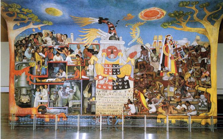
This paper aims to investigate the differences between the level of abstraction achieved by deep convolutional neural networks as compared to the human performance in the context of paining analysis. To synthesize the motivation, let us recall Pablo Picasso words: ”There is no abstract art. You must always start with something. Afterward you can remove all traces of reality”. Art historians and enthusiasts are able to note, while recalling major artistic works through the history, that the level of abstraction steadily increased.

In parallel, in the last period, works that use computer vision techniques to analyze visual art increased with respect to both the quantity and the quality of reported results. Two trends favored these developments. First, there were consistent efforts to digitize more and more paintings, such that modern systems may learn from large databases. Two of such popular efforts are Your Paintings (now Art UK) which contains more than 200,000 paintings tightly connected with historical British culture and WikiArt which contains around 100,000 paintings gathered from multiple national cultures. The databases come with multiple annotations. For this work we are particulary interested in annotations dealing with the painting s subject or scene type. From this point of view, a more complete database is the WikiArt collection, where the labelling category is named genre. The second trend is purely technical and it deals with the development of the Deep Neural Networks, that allowed classification performances that were not imagined before. In this work, we will use the more popular Convolutional Neural Networks (CNN) to recognize the painting genre.

Let us, now, to establish the meaning of genre the relation with scene and with the image subject. A list of definitions for various paintings genres is presented in Table 1. To label a painting into a specific genre, in most of the cases, a user has to identify the subject of that painting. The exceptions are “Abstract Art”, “Design”, “Illustration” and “Sketch and Study”, where the main characteristic is related to the depiction mode. In this majority of cases, subject is related to the scene represented in the work of art. The term “genre” is typical for art domain, and is a more general, including, concept than mere “subject” or ”scene type”. In this work, while referring to paintings, we will use all three with the same meaning of ”genre”. In comparison, for a non-artistic photograph, as there is no artistic intervention in the depiction mode, the subject is more related to the scene, while the genre is hard to be defined. For artistic photos, the “genre” gets meaning again.

Starting from the idea that Deep Neural Networks share similarities with the human vision (Cichy et al., 2016) and the fact that such networks are already proven to be efficient in other perception-inspired areas, like object recognition or even in creating artistic images, we ask ourselves if they can pass the abstraction limit of artistic paintings and correctly recognize the scene type of such a work.

In this paper we will first work with the Residual Network (ResNet) on the standard WikiArt database so to obtain state of the art results. Afterwards, we will test different domain transfer augmentations to see if they can increase the recognition rate; also we will study if the network is capable to pass the abstraction limit and learn from different types of images that contain the same type of scenes. Furthermore, we introduce several alternatives for domain transfer to achieve a dual-task: improve the scene recognition performance and understand the abstraction capabilities of machine learning systems.

Regarding deep networks, multiple improvements have been proposed. In many situations, if the given task database is small, better performance is reachable if the network parameters are previously trained for a different task on a large database, such as ImageNet. Next, these values are updated to the given task. This is called fine–tuning and it is a case of transfer learning. As our investigation is related to a different domain transfer, we will avoid to use both of them simultaneuosly, in order to establish clearer conclusions. To compensate, we are relying on the recent architecture of the Residual Networks (Resnet (He et al., 2016)) that was shown to be able to overcome the problem of vanishing gradients, reaching better accuracy for the same number of parameters, when compared to previous architectures.

1.1 Contribution and paper organization

This paper extends our previous works (Florea et al., 2017a; Badea et al., 2017), being mostly developed from (Florea et al., 2017a), where we had initiated the discussion about the efficiency of various methods to transfer information from the photographic domain to the paintings domain, such that the recognition by CNNs’ of paintings genre is improved. In this paper we significantly extend the discussion, by including other transfer methods and by adding more significant results that allow crisper conclusions. In the second work ((Badea et al., 2017)), we showed that the artistic style transfer remains as efficient even if a reduced number of iterations are performed while over–imposing the style of an artistic painting and the content from a photograph onto a new image, according to the neural style transfer introduced by Gatys et al. 2016.

Overall, this paper claims several contributions along a number of directions. On one direction, we investigate which aspects, comprehensible by humans, hinder the CNNs while understanding a painting genre; subsequently by means of domain transfer, we retrieve information about the internal description and the organization of the painting clusters. In order to accomplish such a task, we annotate artistic photographic images with respect to the scene type related to genres and we stylize a large corpus of photographs using different style transfer methods. All this data will be made publicly available to be used in other research works.

On a second direction, this paper is the first to objectively evaluate the efficiency of the currently popular neural style transfer methods. Currently existing solutions (Gatys et al., 2016; Johnson et al., 2016; Ulyanov et al., 2016; Huang & Belongie, 2017) compare themselves by speed, stability within video sequences or number of transferable styles. By quantifying the improvement while adapting photographs to the painting domain, we reach a surprising conclusion, namely that they are less or at most as efficient as non-neural style transfers solutions. Evermore, a CNN finds as informative the original photographs without any style transfer applied.

The remainder of the paper is organized as follows: section 2 presents previous relevant works, section 3 summarizes the CNN choices made and section 4 will discuss different aspects of painting understanding. Section 5 presents the used databases, while implementation details and results are presented in section 6. The paper ends with discussions about the impact of the results.

2 Related Work

This work investigates the capabilities of CNNs’ to recognize the subject of paintings as compared with the performance of humans. Thus, relevant prior work refers to solutions for object and scene recognition in paintings. As paintings are an abstraction of real images, scene recognition in photographs is also relevant. At last we aim to adapt information from photographs to paintings by means of style transfer.

Object and scene recognition in paintings. Computer based painting analysis has been in the focus of the computer vision community for a long period. A summary of various directions approached, algorithms and results for not-so-recent solutions can be found in the review of Bentowska and Coddington 2010. However, a plurality of works (Agarwal et al., 2015; Karayev et al., 2014; Bar et al., 2014; Florea et al., 2017b) addressed style (art movement) recognition as it is the main label associated with paintings. An intermediate topic is in the work of Monroy et al. 2014 which detected and extracted shapes (associated with objects) but as pre-processing for the final task which was that of restoration.

Object recognition has been in the focus of Crowley and Zisserman 2016 while searching the YourPaintings dataset with learning on photographic data; yet this dataset features “older” art, which is less abstracted than modern art.

Scene recognition in paintings is also named genre recognition following the labels from the WikiArt collection. This topic was approached by Condorovici et al. 2013 and by Agarwal et al. 2015; both works, using the classical feature+classifier approach, tested smaller databases with a few (5) classes: 500 images - (Condorovici et al., 2013) and 1500 images - (Agarwal et al., 2015). More extensive evaluation, using data from WikiArt, was performed by Saleh and Elgammal 2015, which investigated an extensive list of visual features and metric learning to optimize the similarity measure between paintings and respectively by Tan et al. 2016, which employed a fine tuned AlexNet architecture (Krizhevsky et al., 2012) to recognize both style and genre of the paintings.

The process of transferring knowledge from natural photography to art objects has been previously addressed beyond the recent transfer from ImageNet to WikiArt (Tan et al., 2016); yet their solution is general as it is common to use ImageNet pre-trained CNNs on smaller databases. 3D object reconstruction can be augmented if information from old paintings is available (Aubry et al., 2013). Classifiers (deep CNNs) trained on real data are able to locate objects such as cars, cows and cathedrals (Crowley & Zisserman, 2016) if the artistic rendering is not very abstract. The problem of detecting/recognizing objects in any type of data, regardless if it is real or artistic, was named cross-depiction by Hall et al. (Hall et al., 2015); however the problem is noted as being particular difficult and in the light of dedicated benchmarks (Cai et al., 2015), the results show plenty of space for improvement.

A significant conclusion that arises is that all solutions that showed some degree of success did it for older artistic movements, where scene depiction was without particular abstraction. To our best knowledge there is no reported significant success for (more) modern art.

Scene recognition in photographs. Scene recognition in natural images is an intensively studied topic, but under the auspices of being significantly more difficult than object recognition or image classification (Zhou et al., 2014). We will refer the reader to a recent work (Herranz et al., 2016) for the latest results on the topic. We will still note that the introduction of the SUN database (Xiao et al., 2010) (followed by the subsequent expansions) placed a significant landmark (and benchmark) on the issue. In this context, it was shown that using domain transfer (e.g from the Places database), the performance may be improved (Zhou et al., 2014).

Style transfer. Any image claiming artistic representations adheres to some non-trivial ideas about content, color and composition; these ideas are often grouped in styles. It has been an important theme in computer vision (Bae et al., 2006) to develop methods that are able to transfer the style from an artistic image to a normal, common image. The methods are called style transfer. Currently, the methods may be classified as non-neural (such as the Laplacian style transfer (Aubry et al., 2014)) and neural artistic style transfers, initiated by the method of Gatys et al. 2016. We will detail these algorithms in section 4. For the moment, we will note that the efficiency of the transfer was quantified, till now, only subjectively as that it was not rigourously defined the concept of the style so to evaluate objectively.

Scene recognition by humans. While it is beyond the purpose of this paper to discuss detailed aspects of the human neuro-mechanisms involved in scene recognition, following the integrating work of Sewards 2011 we stress only one important aspect: compared to object recognition, where localized structures are used, for scene recognition the process is significantly more tedious and complex. Object recognition ”is solved in the brain via a cascade of reflexive, largely feedforward computations that culminate in a powerful neuronal representation in the inferior temporal cortex” (DiCarlo et al., 2012). In contrast, scene recognition includes numerous and complex areas, as the process starts with peripheral object recognition, continues with central object recognition, activating areas such as the entorhinal cortex, hippocampus and subiculum (Sewards, 2011).

Concluding, there is a consensus, from both the neuro-science and the computer vision communities that scene recognition is a particularly difficult task. This task becomes even harder when the subject images are heavily abstracted paintings produced within the movements of modern art.

3 CNNs: Architectures and Training

Following AlexNet (Krizhevsky et al., 2012) performance in the ImageNet challenge, in the recent years we have witnessed a steep increase in popularity of Convolutional Neural Networks (CNNs) when considering the task of image classification. Especially after Donahue et al. 2014 showed that ImageNet pre-trained CNNs provide very good descriptors, it is very hard to find a large-enough database where state of the art performance is not related with CNNs. As such, the bulk of our experiments revolve, in one way or another, around the CNN algorithms, either as direct classification methods or as auxiliary tools.

The first network architecture tested in this work is AlexNet, proposed by Krizhevsky et al 2012. This architecture features 5 convolutional layers followed by 3 fully connected layers. The size of the receptive fields is large ($11\times 11$), in comparison to more recent architectures; the design is optimized for the use of two parallel GPUs, although currently it easily fits on a single GPU. Even though it has been visibly surpassed by other networks, it still remains a main reference point in all architecture comparisons.

A more powerful architecture is represented by the VGG-type networks, proposed by Simonyan and Zisserman 2015. In contrast to AlexNet, this design features smaller receptive fields ($3\times 3$), but with a stride between regions of only 1. These decisions have led to the possibility of increased depth, by stacking sequentially up to 5 convolutional layers, and, subsequently, to higher performance than AlexNet. Although we do not use this network for direct classification, the stacked convolutional layers of VGG -19 trained on ImageNet produce very efficient feature descriptors, and, thus, are heavily used by the style transfer algorithms (Gatys et al., 2016; Johnson et al., 2016).

In the remainder of the paper, for the task of classification, we will use the Residual Network (ResNet) (He et al., 2016) architecture, with 34 layers. All the hyper-parameters and the training procedure follow precisely the original ResNet (He et al., 2016). Nominally, the optimization algorithm is 1–bit Stochastic Gradient Descent, the initialization is random (i.e. from scratch) and when the recognition accuracy levels on the validation set, we decrease the learning rate by a factor of 10. The implementation is based on the CNTK library.

4 Painting Understanding and Domain Transfer

The main task of this work is to generate results about the understanding of the machine learning systems (in our case deep CNN) grasp of art. In such a case, one needs tools to ease the comprehension of the system internal mechanisms.

For CNNs, the most popular visualization tool has been proposed by Zeiler and Fergus 2014 by introducing deconvolutional layers and visualizing activations maps onto features. Attempts to visualize the CNNs, for scene recognition, using this technique, indicated that activations are related to objects. Thus it lead to the conclusion that multiple object detectors are incorporated in such a deep architecture (Zhou et al., 2015). This means that high activations were triggered simultaneously in multiple parts of an image, being thus rather spatially vague. In parallel, visualization of activations for genre (Tan et al., 2016) have shown that, for instance, the landscape type of scene leads to activating almost the entire image, thus being less neat to draw any conclusion. Consequently, we tried a different approach to investigate the intrinsic mechanisms of deep CNNs. Our approach exploits domain transfer and simply correlates the final results with the training database.

Given the increased power of machine learning systems and the limited amount of data available to a specific task, a plethora of transfer learning techniques appeared (Lu et al., 2015). Transfer learning is particularly popular when associated with deep learning. First, let us recall that the lower layers of deep nets trained on large databases are extremely powerful features when coupled with a powerful classifier (such as SVM) and may act as feature selectors, no matter the task (Donahue et al., 2014). Secondly, the process of fine tuning deep networks assumes using a network that has been pre-trained on another database, and, with a small learning rate, adapting it to the current task.

In contrast, the concept of domain transfer or domain adaptation appeared as an alternative to the increase of the amount of information over which a learner may be trained directly (without fine tuning) in order to improve its prediction capabilities. Many previous solutions and alternatives have been introduced. We will refer to the work of Ben-David et al. 2010 for theoretical insights on the process.

It has been shown that domain transfer is feasible and the resulting learner has improved performance if the two domains are adapted. In this context one needs to mention the work of Saenko et al. 2010 that proved that using a trained transformation, the domain transfer is beneficial.

In our case, the target domain is the artistic painting domain, while for the source domain we consider several alternatives: consumer photographic image domain (represented by images from the SUN database), artistic photographic image domain (with instances from the Photo-Artist database), and a combination of features from the painting domain (taken from the ”older”, less abstract styles of paintings); these will be detailed further in section 5 and, respectively, in 6.

For the domain adaptation function we investigate several alternatives. As a visual distinctive characteristic of painting is the style, the investigated functions are in the category of style transfer methods. As they are a key concept to our work, in the next subsection we will detail them.

4.1 Style transfer

Following the seminal work of Reinhard et al. 2001 the idea to transfer elements from a reference image, with an artistic value, to a subject one increased in popularity. The main concepts introduced then still stand: first, both images are represented into a space that offers a meaningful description with respect to transferable elements; next, the subject image is altered such that it fits into the description of the reference image. Quite often the second step implies matching the estimated probability density functions (i.e histograms) of the two images. A simple version 2001; 2017 is to assume the distribution in the feature space to be Gaussian, independent (or at least uncorrelated) with respect to the dimensions. Such an assumption is a sword with two edges: on one side, the feature space should be constrained to follow the decorrelation assumption, but, on the other hand, the matching process is very simple as only the mean and the variance on each feature dimension needs to be fitted.

While in the original work (Reinhard et al., 2001), the envisaged transferable element is color, later, the style of the image was approached (Bae et al., 2006). Prior to popularization of CNNs, image descriptors were based on manually–set filter weights; a prominent is the case of the Laplacian style transfer (Aubry et al., 2014). In the last period, the spectacular results showed by Gatys et al. 2016 helped the so called Neural Style Transfer methods to gain in popularity.

In the next subsections we will review the formalization of the main style transfer methods; $\mathbf{S}$ will denote the subject image, while $\mathbf{R}$ the style reference image. In some solutions, $\mathbf{S}$ is altered to mimic the style from $\mathbf{R}$, in others, a third image $\mathbf{X}$, is built from scratch to match the content from $\mathbf{S}$ and the style from $\mathbf{R}$.

4.1.1 Laplacian style transfer

Following the findings of Sunkavalli et al. 2010, the complex transfer process produces better results if it is carried separately on different levels of details from the two images. The most simple form to have various details of an image is to use a pyramidal representation. The Laplacian style transfer (Aubry et al., 2014) assumes a Laplacian pyramidal representation with multiple levels. On each level the style transfer is implemented as gradient transfer. Nominally, at each pixel, $\mathbf{p}$, in each level of the pyramid, given a neighborhood $\mathbf{q}$, the set of gradients in the two images is $\nabla S_{\mathbf{p},\mathbf{q}}$ (for the subject image) and $\nabla R_{\mathbf{p},\mathbf{q}}$ (for the reference image). The transfer is implemented by iteratively correcting the local point $S(\mathbf{p})$:

$$\begin{array}[]{cl}\mathbf{S}_{n}(\mathbf{p})&=r(\mathbf{S}_{n-1}(\mathbf{p}));\enspace r(i)=g+sign(i-g)t(|i-g|);\\ t(i)&=CDF^{-1}_{[\nabla\mathbf{R}(\mathbf{p})]}\left(CDF_{[\nabla\mathbf{S}(\mathbf{p})]}(\mathbf{p})\right)\end{array}$$ (1)

where CDF is the cumulative density function computed on the image, $r(\cdot)$ is the transfer function, while $\mathbf{S}_{1}(\mathbf{p})$ is the initial local pixel of the subject image and $\mathbf{S}_{n}(\mathbf{p})$ is the same value at iteration $n$. The mapping needs to be done iteratively, as in practice the CDF is approximated by the local cumulative histogram on a discrete support of values. Typically, 10 iterations suffice.

4.1.2 Neural style transfer algorithm

The algorithm proposed by Gatys et al. 2016 aims to transpose the style by representing an image into a space where content and style are separable. This is achieved by using the feature representation offered by the layers of a convolutional network architecture that do not have skip connections (e.g. VGG–19). The choice for this representation originates in the observation that higher layers (i.e. closer to the fully connected and to the classification layers) will focus on high-level features, thus onto content (the focus is on objects, not on the actual pixels), while the first layers can be used to reconstruct the image with accurate pixel values.

Differently with respect to previous works which adjust the subject (content) image, the original neural style algorithm (Gatys et al., 2016) starts from a white noise image, X, which is modified in order to match the over imposed statistics.

Starting from the white noise image, the method employs gradient descent to smoothly adjust values in order to match the content and style of the desired source images. The global loss function is a linear combination between two other loss functions used for content and, respectively, the style matching. In the neural style transfer algorithm, the subject image will provide the content matching, $\mathbf{S}$, while the generated image is $\mathbf{X}$. Considering the activations $F_{ip}^{l}$ ($P_{ip}^{l}$) of the $i^{th}$ filter on the $l^{th}$ layer at position $p$ in a CNN representation of $\mathbf{S}$ (and respectively $\mathbf{X}$), the loss function with respect to content can be defined as:

$$L_{content}(\mathbf{S},\mathbf{X},l)=\frac{1}{2}\sum_{i,j}(F_{ip}^{l}-P_{ip}^{l})^{2}$$ (2)

To underline the correlations between activations, the algorithm uses the Gram matrix; $G_{ip}^{l}$ is the inner product between the vector versions of the $i^{th}$ and $p^{th}$ feature maps of the $l^{th}$ layer:

$$G_{ip}^{l}=\sum_{k}F_{ik}^{l}F_{pk}^{l}$$ (3)

With the Gram matrix defined, the contribution of each layer is brought into discussion. The $l^{th}$ layer is composed of $N_{l}$ feature maps of size $M_{l}$. Thus, considering, besides $\mathbf{X}$, the style source image $\mathbf{R}$, the Gram representations $A^{l}$ and $G^{l}$ are computed for layer $l$. The contribution of a certain layer and the total style loss function are:

$$E_{l}=\frac{1}{4N_{l}^{2}M_{l}^{2}}\sum_{i,j}(G_{ip}^{l}-A_{ip}^{l})^{2}$$ (4)

$$L_{style}(\mathbf{A},\mathbf{X})=\sum_{l=0}^{L}w_{l}E_{l}$$ (5)

The total loss function, which takes into account both content and style is a linear combination of the two aforementioned components:

$$L_{total}(\mathbf{X},\mathbf{S},\mathbf{R})=\alpha L_{content}(\mathbf{S},\mathbf{X})+\beta L_{style}(\mathbf{A},\mathbf{X})$$ (6)

where $\alpha$ and $\beta$ are manually picked weights.

The dramatic visual impact of the original visual style transfer method encouraged other works to address the same subject. Li et al. (Li et al., 2017) showed that, in fact, this version of style transfer minimizes the Maximum Mean Discrepancy (MMD) with the second order polynomial kernel thus implementing another version of matching the feature distributions. Maximum Mean Discrepancy (MMD) is a test statistic for the two-sample testing problem, where acceptance or rejection decisions are made for a null hypothesis (Gretton et al., 2012); thus, in other words, a minimum MMD enforces that two distributions, in this case that of the image $\mathbf{X}$ and that associated with the reference images ($\mathbf{S}$ for style and $\mathbf{R}$ for style) are similar enough, within a statistical relevance limit. The last work (Li et al., 2017) indicates that the relation of the neural style transfer abides to the original principle stated by Reinhard et al. 2001, namely of feature distribution matching. The neural style transfer (Gatys et al., 2016) implements an approximation of the exact solution, which would have been given by inverting and composing the Cumulative Density Functions (CDF).

In an attempt to accelerate the transfer, Ulyanov et al. 2016 and Johnson et al. (Johnson et al., 2016) learned the inverse mapping by a deep CNN. Yet this approach has the disadvantage that only a specific reference image equivalent CDF may be learned by the CNN; another style from another reference image requires another CNN. Thus, this approximation restricts the number of transferable styles to the number of CNNs trained. The limitation was very recently approached by Huang and Belongie 2017, which assumes independent Gaussians and thus match only the mean and variance (to obtain the statistical match) following by training a CNN to approximate the multivariate Gaussian CDF and do the inverse mapping.

Although it is faster, the CNN learning of the inverse CDF as in (Johnson et al., 2016; Ulyanov et al., 2016) dramatically limits the number of transferable styles, making the concept ineffective as domain adaptation method. The Gaussian matching (Huang & Belongie, 2017), while being able to transfer an infinity of styles, still imposes two approximations that have an effect on the final image quality. Concluding, the original neural style transfer (Gatys et al., 2016) remains the most viable candidate for domain adaptation between the photographic image domain and the paintings domain.

4.2 Comparison Between Neural and Laplacian Transfers

While the Laplacian and Neural style transfer are built on different paradigms (neural vs. non-neural), we stress that the two methods share similar concepts. First, let us note that the pooling paradigm from the CNN is similar with the downsampling used in the Laplacian pyramid. Noting that the best results for the neural style transfer are achieved using a VGG-19 architecture, this implies an input image of $224\times 224$; the VGG-19 has 4 pooling layers between convolutional layers, thus offering a 5 level pyramidal representation. For the same image input, the Laplacian transfer uses 7 levels, thus going for coarser style too. In each such pyramidal level, the VGG stacks 2 to 3 convolutions, while the Laplacian uses only one.

Another aspect is related to the used filters. For the Laplacian filters, the weights are preset, always having the same values, while for the neural style transfer, the weights are learned while trying to classify on the ImageNet task. It has been shown that the CNN lower level filters are similar to standard gradient filters (Fischer et al., 2014), yet those from upper levels have no such correspondence. In this point, one should note that CNN architectures use multiple filters in parallel (the VGG from 64 in the bottom layer to 512 in the upper ones), while the Laplacian only 1. This huge difference ensures that a much richer description is available for the neural transfer.

The last aspect taken into account for the comparison is the procedure used for matching the distributions. The original Neural Style transfer goes for minimizing the MMD, which is to ensure that the multi-dimensional feature distributions of the image to change and of the reference image do match from a statistical point of view. The Laplacian goes for the exact solution. Yet, the inverting of the CDF in the Laplacian is also imperfect, as the computed “cumulative density function” is only an approximation of the true CDF, aspect enhanced by the significant number of iterations, which are required to fill the discontinuities. Another point is that the full inversion is possible because the Laplacian uses 1D feature description, thus being less richer than the multi-dimensional one used for the neural version.

Concluding, just by looking at the richness of the two algorithms, the neural style transfer may be grossly perceived as a significant step ahead with respect to the Laplacian counterpart.

5 Databases

For the various experiments undertaken, several databases have been employed. These are either a collection of digitized paintings, either a collection of digital photographs. In the next paragraphs we summarize their main characteristics.

5.1 WikiArt database

The WikiArt is a collection of digitized paintings used to popularize art. It is in continuous expansion, as every day new works of art are added. The version used is the same as in (Karayev et al., 2014) and it contains approximately 80,000 digitized images of fine-art paintings. We note that this version is highly similar to ones used by prior art, to which we compare against.

The images are labelled within 27 different styles (cubism, rococo, realism, fauvism, etc.), 45 different genres (illustration, nude, abstract, portrait, landscape, marina, religious, literary, etc.) and belong to more than 1000 artists. To our knowledge this is the largest database currently available that contains genre annotations. For our tests we considered a set that contains 79434 images of paintings.

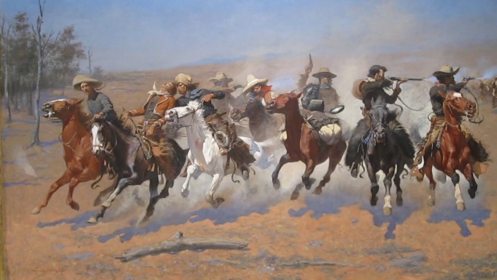
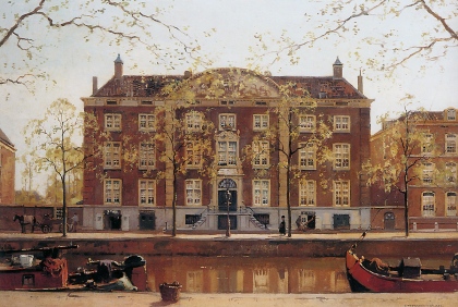
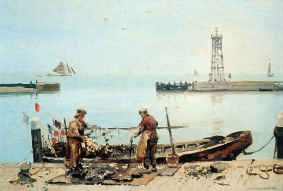
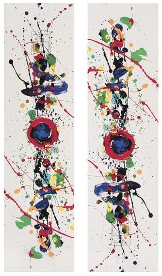
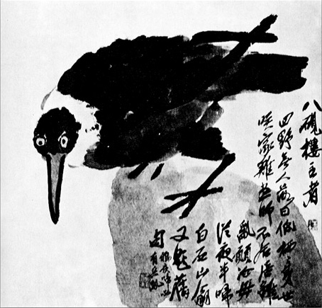
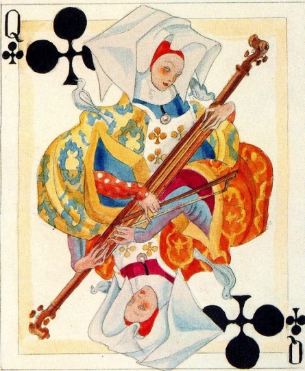
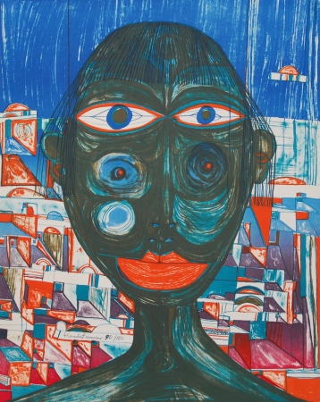
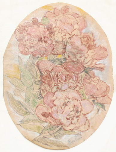
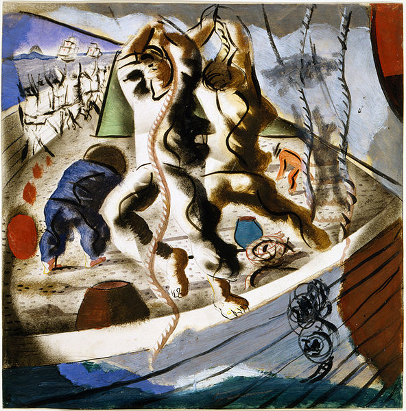
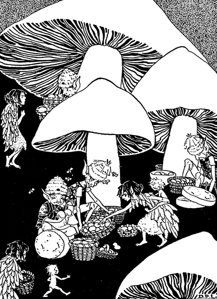
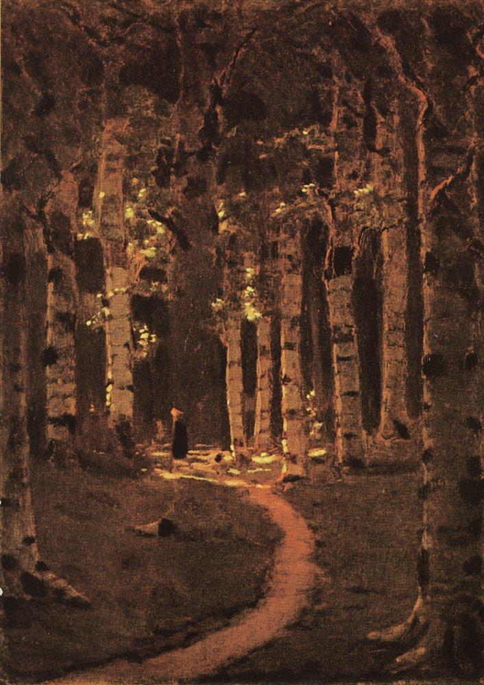
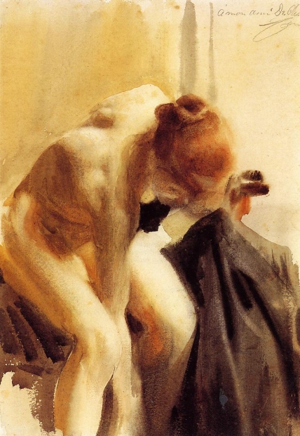
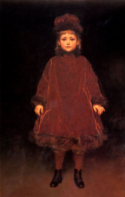
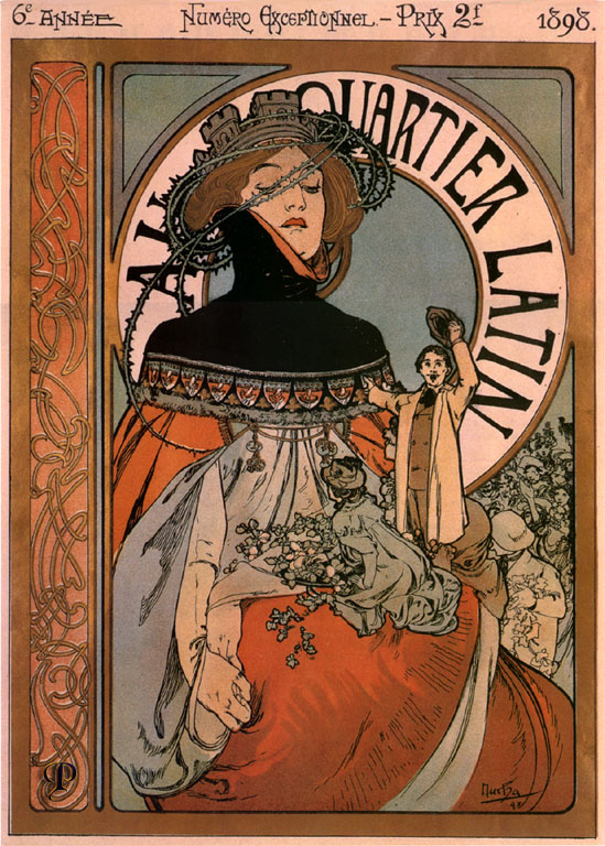
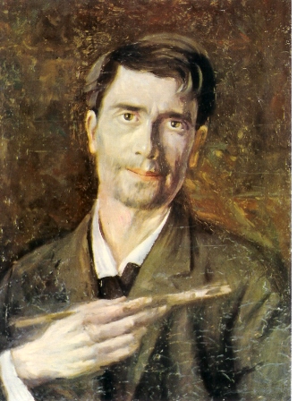
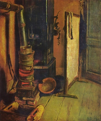
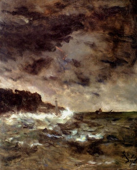
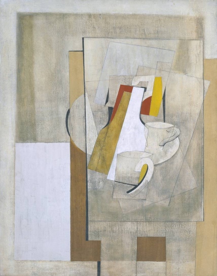
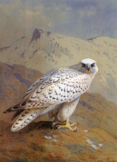
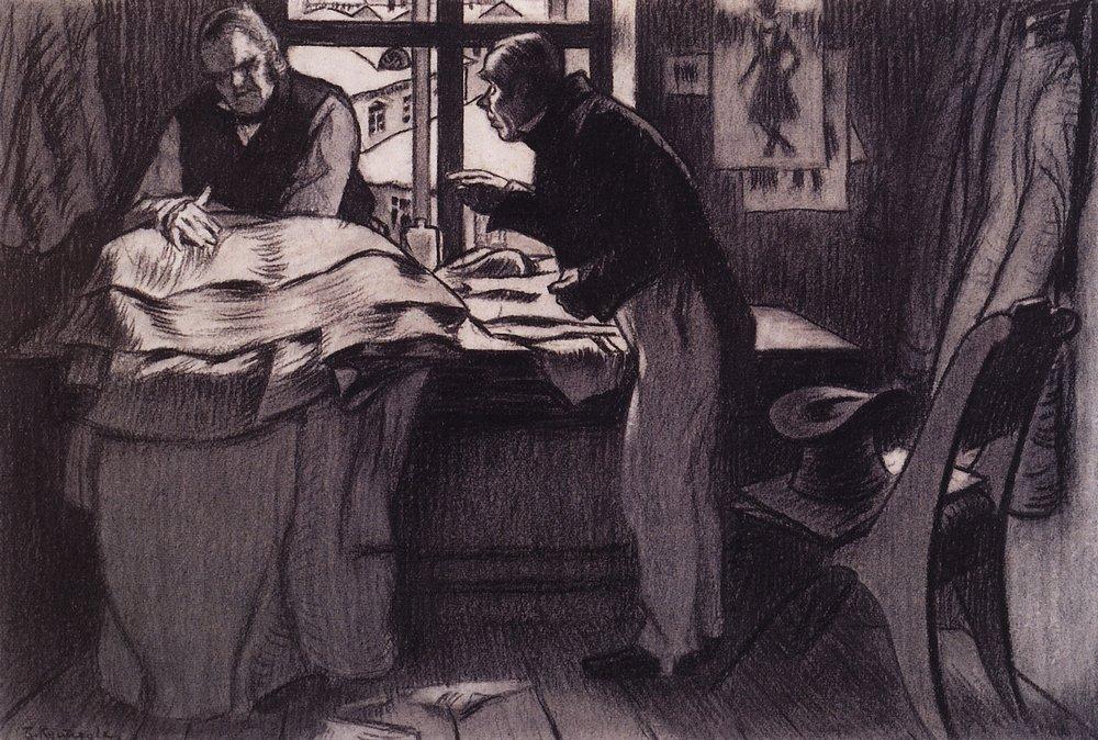
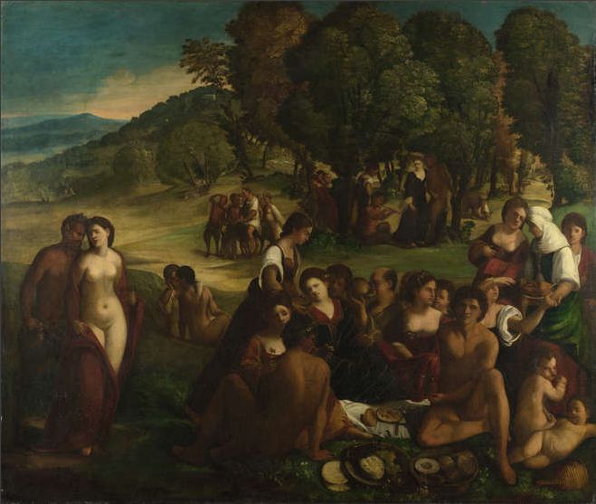
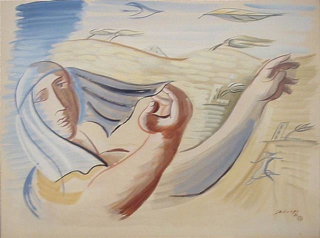
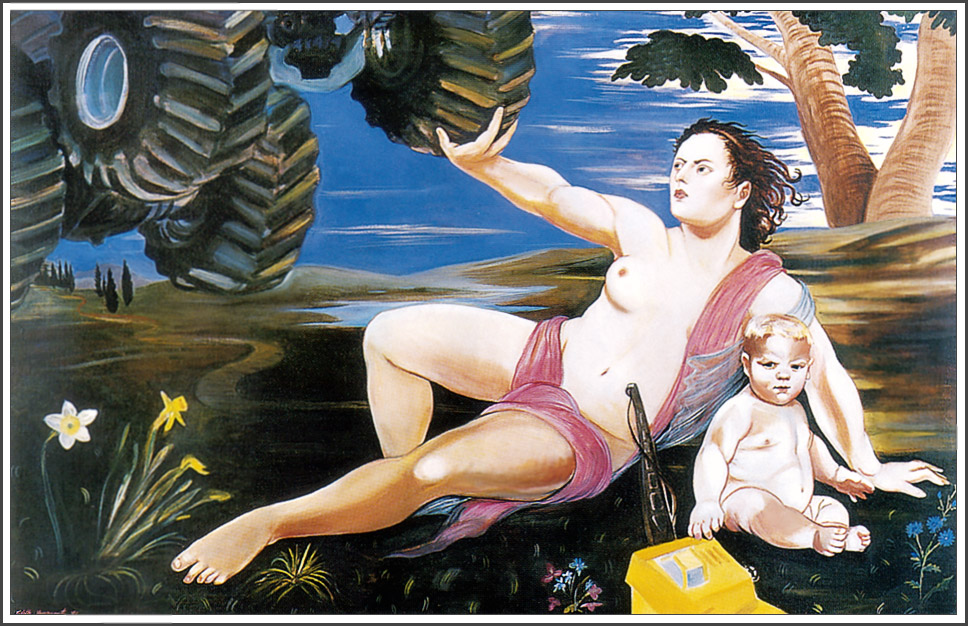
In WikiArt some of the genres were not well represented (i.e. less than 200 images) and we gathered them into a new class called “Others”. This led to a division of the database into 26 classes illustrated in Figure 1. The names of the classes and the number of training and testing images in each class can be seen in Table 1. Furthermore, as the genre label is not explained in prior works, we also contribute with an explanation of the genre meaning; these explanations are collected from an Internet encyclopedia.

The list of genres that counted less than 200 examples and are included in the ”Others” class contains, among others: ”advertisement” – 94 examples – illustrate a work of art designed to market a product; ”capriccio”(194) – depict architectural fantasies, placing together buildings and/or elements in fantastical combinations; “caricature”(184) - variation of sketch, but with intended comical effect; “cloudscape” (162) - depicting clouds or sky; ”miniature” (79) - small paintings, typically originating in early middle age in the Byzantine or Central Asian empires; ”mosaic” (17) – images made from the assemblage of small pieces of colored materials; ”panorama”(17) – massive artworks that reveal a wide, all-encompassing view of a particular subject; ”pastorale” (80) - illustrates segments of life from shepherds herding livestock around open areas; “quadratura” (19) - an image based on techniques and spatial effects to create an illusion of three-dimensional space; “tessellation” (122) - images of aperiodically patterns from M. C. Escher; “vanitas”(34) - symbolic works of art, associated with the still life and “veduta” (188) – which are a highly detailed large-scale paintings.

We note that annotation is weak, as one may find arguable labels. For instance “literary” and “illustration” categories may in fact have “landscape” subjects. However, as this distribution matches practical situations, we used the database as it is, without altering the annotations.

After observing the main characteristics of paintings genres in Table 1, one may conclude that the task is similar with the identification of a scene type in a photograph. Basically, in most cases, the genre is given by the topic (subject) rendered in the artwork. Under these circumstances, especially to specific genres, we consider that appropriate for domain transfer, are images labelled for scene content.

Table 1: Overview of the genre organization of the WikiArt database and the explanation of the label meaning. We have marked only genres with more than 200 images.

	Genre	No. imgs.	Description
1	Abstract Art	7201	Uses shapes, forms etc. to replace accurate representations
2	Allegorical Painting	809	Expression of complex ideas using another subject
3	Animal Painting	1233	Paintings which depict animals
4	Battle Painting	273	The main subjects are battles and wars
5	Cityscape	4089	Works which contain cities or other large communities
6	Design	1577	Conceptual schemes of objects and structures
7	Figurative	1782	Forms inspired by objective sources, but altered
8	Flower Painting	1270	Paintings of flowers
9	Genre Painting	10984	Scenes of everyday life
10	History Painting	656	Depictions of historical events
11	Illustration	2493	Visual representations usually meant for books, magazines, etc.
12	Interior	511	Paintings depicting interiors of structures
13	Landscape	11548	Contains representations of land, or other natural scenes
14	Literary Painting	418	Subject taken from literary work
15	Marina	1385	These paintings show scenes from docks or ports
16	Mythological Painting	1493	Inspired by mythology
17	Nude Painting	1758	Paintings which contain nudes
18	Portrait	12926	Images of real individuals
19	Poster	229	Works which are usually intended for advertising
20	Religious Painting	5703	Inspiration is drawn from religious scenes
21	Self-Portrait	1199	The subject of the painting is the artist
22	Sketch and Study	2778	Drawings done for personal study or practice
23	Still Life	2464	Images which depict inanimate objects
24	Symbolic Painting	1959	Content suggested by symbols in the forms, lines, shapes, and colors
25	Wildlife Painting	259	Paintings of natural scenes, including animals in their habitats

Allegorical Battle Cityscape Genre

Abstract Animal Design Figurative Flower History

Illustration Landscape Nude Portrait Poster Self-portrait

Interior Marina Religious Still Wildlife

Literary Mythological Sketch Symbolic

Figure 1: Examples illustrating the 25 Genre categories from the WikiArt collection. “Others” is not illustrated. Note that some categories can still be confused with other, such as “Mythological” with “Symbolic” or “Religious”.

5.2 Natural Scenes Databases

As a first additional source of data we have considered images from the SUN (Scene Understanding) database (Xiao et al., 2010). In its original form, it contains 899 classes and more than 130,000 images. Yet, only a few classes, which have a direct match with the content of the WikiArt genre database, were selected. These classes and the number of images in each one that were added in the training process at some step are: “Cityscape” -2903 images, “Flower” -229, “Landscape”- 7794, “Marina” -1818.

Supplementary, since portraits are a very common type of paintings, we have retrieved 5993 images from the Labelled Faces in the Wild (LFW) database (Huang et al., 2007). Again, these images are a mere rendering of one’s face without any artistic claim. In the next section, if it is not specified otherwise, these portraits will be associated with SUN photos. In total we have 20,075 normal photographs.

As a particular characteristic of the images from the SUN/LFW databases is that they were not selected for their artistic value, but strictly for their adherence to one of the scene classes tightly associated with studied genres. Artistic value, if there is any, is merely coincidental. Also there is no abstraction in this data.

5.3 Photo-Artist Data Set

Thomas and Kovashka 2016 have collected a large database of artistic photographs. Unlike the images from the SUN – LFW database, in this case, each image has an important artistic value, and its author is broadly accepted as an artist. The artistic value is encoded in the composition, framing, colors, or in other elements that are harder to objectively quantify. Yet this database was not labelled with respect to subject or scene composition.

From this large collection, we have selected and labelled a subset of 19,573 images distributed as follows: “Cityscape”–8068 images, “Interior”–3036 images, “Landscape”–4467 images, “Portrait”–4002 images.

5.4 Stylized Images

The most striking visual difference between photographs and paintings is the style of representing the subject within the paintings. In an effort to transfer knowledge between the two image types, we have stylized some sets of images as follows:

• images from the Photo-Artist database were stylized with Laplacian style transfer;

• images from the Photo-Artist database were stylized with neural style transfer.

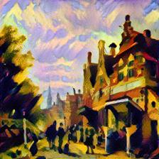
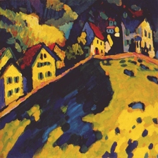
• images of paintings with classical styles, that have a realistic depiction of reality, have been stylized using the neural transfer method and according to the styles of modern abstract art movements.

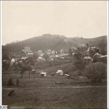
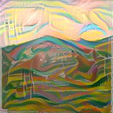
Example of stylized paintings may be seen in Figure 2. We have not stylized images from SUN–LFW database, as (one may see further in Table 4) their performance was not better than those of Artistic–Photo and the process is very tedious.

For the reasons previously mentioned, among neural solutions, we have used the original neural style transfer method (Gatys et al., 2016). The motivation for trying to transfer the abstract style onto realistic paintings lies in the observation that, over time, the paintings adheres to the same favorite subjects.

Artistic Photo Laplacian stylized image Reference painting

Classic style painting Neural stylized image Reference painting

Artistic photo Neural stylized image Reference painting

Figure 2: Examples of the stylization. The left hand column shows the content image, the center column shows the stylized image, while the right hand column contains the style reference painting. In this case, the images are at the resolution used by the CNN ($224\times 224$).

The process of neural stylization using the original neural solution is time consuming. For the initial tests (Florea et al., 2017a) we have used a NVIDIA GTX 980 Ti and a NVIDIA K40; in this case, the stylization of an image took 2-10 minutes, which matches the more recent reports in (Chen & Schmidt, 2016). Further acceleration (Badea et al., 2017) and the use the faster NVIDIA GTX 1080 Ti allows, currently, faster stylization with a duration scaled down to 30 sec; yet this is still slow considering the size of the databases, so that one will not produce an extremely large quantity of images.

6 Implementation and Results

The main goal of this work is to study the performance of the CNNs in recognition of a paintings’ genre and, in parallel, to investigate various ways in which this performance can be increased. This includes experiments on the classification methods themselves, in order to establish both the state of the art performance and a baseline for further experimentation. Afterwards, we follow with experiments on various alterations brought to the database in the context of domain transfer.

6.1 Baseline and comparison with prior work

Genre recognition has been previously attempted using the WikiArt collection. We show that the used current procedure leads to slightly superior performance when compared to previously proposed solutions. Furthermore, as the list of prior art is not too rich, we have tested some classical solutions to establish more firmly the baseline performance.

Agarwal et al. 2015, Tan et al. 2016 and Saleh and Elgammal 2015 used the WikiArt database for training and testing in order to classify paintings into different genres. While the first two used a very small subset, the later two solutions focused on 10 classes from the entire database, namely: Abstract, Cityscape, Genre, Illustration, Landscape, Nude, Portrait, Religious, Sketch and Study and Still life; in total their subset gathered $\sim$63,000 images.

We have adopted the division (training and testing) from Karayev et al. 2014 as working with a complete version of WikiArt. Furthermore, we stress that in our case the images from training and testing are completely different and are based on a random selection.

In order to compare our results to the ones reported by the mentioned previous works, we have selected the same classes of paintings for training and testing. While in the case from (Saleh & Elgammal, 2015) the test-to-train ratio is mentioned, in (Tan et al., 2016), it is not. Under these circumstances and against our best efforts, the comparison with prior art is, maybe, less accurate.

The results from Table 2 show that the proposed method gives slightly better results than previous method (Tan et al., 2016), building upon the difference that they use a smaller fine–tuned (i.e. initialized on ImageNet) network (AlexNet), while we have used a larger one, based on the improved residual connections paradigm, but initialized from scratch. Also, the previous work used database augmentation while, for this result, we have not. The difference between here used ResNet-34 and the previously used AlexNet is above the stochastic margin, as we will discuss later. Furthermore, we report the average performance over 5 runs. Thus we may emphasize that our efforts produced state of the art genre recognition on the WikiArt collection.

On the 26-class problem, which will be furthered explored in the remainder of the paper, the residual CNN is able to retrieve better performance than classical solutions. In this test, the classical solutions coupled pyramidal Histogram of Oriented Gradients (pHog) (Dalal & Triggs, 2005) or pyramidal Local Binary Pattern (pLBP) (Ojala et al., 2002), as features, with a SVM for classification. The SVM uses radial basis function and we performed the grid searched for the best $\gamma,C$ parameters. Only features extracted from lower layers of a CNN (DeCAF) provide a description that is competitive with CNNs. Compared to our previous work, where we have reported 59.1% accuracy, the improved performance is due to better hyperparameter tuning. Currently, our effort produced state of the art performance on the 26 class problem.

Table 2: Comparison with state of the art methods. The table is horizontally split to group solutions that have used databases with similar size. Acronyms: BOW - Bag of Words, ITML - or Iterative Metric Learning; pHoG - HoG pyramid as in (Dollár et al., 2014); pLBP - LBP pyramid implemented in VLFeat (Vedaldi & Fulkerson, 2010) DeCAF (Donahue et al., 2014) assumes the first 7 levels of AlexNet trained on ImageNet. With italic we marked our proposed solution while with bold the top performance.

Method	No. classes	No. images	Test ratio	Accuracy (%)
Agarwal et al. 2015 - SIFT+BOW	5	1500	10%	82.53
Agarwal et al. 2015 - ensemble				84.46
Saleh and Elgammal 2015 - Classemes+Boost	10	63.691	33%	57.87
Saleh and Elgammal 2015 - Classemes+ITML				60.28
Saleh and Elgammal 2015 - Classemes+Fusion				60.28
Tan et al. 2016 AlexNet - scratch			n/a	69.29
Tan et al. 2016 CNN- finetune				74.14
Proposed - ResNet 34 - scratch			20%	75.58
pHoG + SVM	26	79,434	20%	44.37
pLBP + SVM				39.58
DeCAF + SVM				59.05
AlexNet - scratch				53.02
ResNet 34 - scratch (Florea et al., 2017a)				59.1
Proposed - ResNet 34 - scratch				61.64
Proposed - ResNet 34 - scratch + augmentation				63.58

Database Basic Augmentation. Besides using domain transfer and domain adaptation, one may improve the recognition performance by adding the original images modified by basic image processing techniques. The processing methods that have produced positive effects are flipping and slight rotation. The flipped versions are all horizontal flips of the original images. Regarding the rotations, all images have been rotated either clockwise or counterclockwise with $3^{0}$, $6^{0}$, $9^{0}$ or $12^{0}$. Adding noise, slight tone adjustment or small translations did not help.

When the size of the training database doubled, the improvement in recognition performance was of 2%, reaching $63.58\%$ while doubling the training time too. We consider the increase too small, so in the remainder of the experiments we have used only the original paintings without basic augmentation.

Table 3: Top–$K$ accuracy for genre recognition rate in the 26-case scenario. Top–$K$ means that a positive recognition is achieved for an example, when any of the any the CNN model $K$ highest probability answers match the expected answer.

K	1	2	3	4	5
Recogn.[%]	61.64	76.24	82.14	88.46	90.09

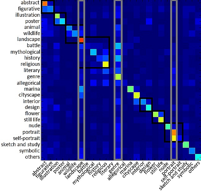
Confusion Matrix. The confusion matrix for the best performer on the 26-class experiment is presented in Figure 3. We have marked classes that are particularly confused. It should be noted that from a human point of view, there is certain confusion between similar genres such as historical$\leftrightarrow$battle$\leftrightarrow$religious, portrait$\leftrightarrow$self portrait, poster$\leftrightarrow$illustration, animal$\leftrightarrow$wildlife etc. Some of these confusable images are, in fact, shown in Figure 1.

Consequently, the Top–$K$ error may also show relevance, as in many cases there are multiple genre labels that can be truthfully associated with one image. The performance with respect to $K$ is presented in table 3. One may note that greater improvement is from Top–1 to Top–2. For the best proposed alternative, ResNet with 34 layers, the Top-5 error is 9.91% - corresponding to 90.09% accuracy. For the 10-class experiment the Top–5 accuracy is 96.75%.

Figure 3: The confusion matrix for the 26 class. We have grouped and marked confusion classes.

Stochastic Effect. This test studied the effect of the stochastic nature of the CNN. Factors such as the random initialization of all the parameters can influence the results of any considered network. We ran the ResNet–34 several (5) times on the 26 classes and the accuracy results had a mean of 61.64% (Top- 1 accuracy) and a standard deviation of 0.33%. The results underline the fact that even though there is some variation caused by randomness, it does not influence the system significantly.

On the other hand, if alternative solutions show variation smaller than 0.33% (“stochastic margin” as we named it), one may argue that these are not relevant to draw conclusions.

For the following experiments we will refer solely to the 26 classes scenario, as it is the most complete. We recall that the baseline performance (and also the best) is 61.64%.

6.2 Influence of the artistic style

Prior art (Zhou et al., 2015) suggests that even in the case of the scene rendered in photographs, in fact, a deep network builds object detectors and can recognize objects presented in a way seen before. These conclusion are based on the viewing method of the CNN filters based on deconvolution (Zeiler & Fergus, 2014). In the case of realistic scenes, Zhou et al. 2015 showed that filters activation is grouped on certain objects in association with a certain class. In the case of paintings’ genre, Tan et al. 2016, using the same visualization technique, showed much more sparsity.

In the same, the deconvolution method has no procedure to identify the failure; in other words there is no way to prove that nothing in particular influences the decision on one class, but rather the small, easy–to–neglect weights, exploited in Distillation – Dark Knowledge (Hinton et al., 2015). To avoid this potential uncertainty, our experiments focus directly on the network output, when the training set was adjusted into a specific direction.

With regard to the artistic style, we have performed two experiments. In the first one, we separate the training and testing based on style, thus asking the CNN to generalize across style, while in the second we have reviewed the baseline performance with respect to style.

For the first experiment, considering the full 79,434 images genre database, we selected all the images that are associated with Cubist and Naive Art styles and placed them in testing, resulting in 4,132 images for evaluation and 75,302 for training. Although numerically this is a weaker test than the baseline, as the training set is larger, the results are considerably worse: 50.82% Top–1 accuracy and 82.10% Top–5. We consider that this drop (from 61.64% - Top–1 and 90.99% Top–5) is due to the fact that these particular styles are rather different from the rest and the learner had no similar examples in the training database. Also these results argue for a style oriented domain adaptation.

The second experiment benefits from the fact that WikiArt images are annotated with multiple labels categories, and one of these category is the style. Thus given the baseline framework (i.e. keeping the same training and testing sets), we retrieve the genre recognition rate with respect to style (artistic movement). The results are showed in Figure 4.

Figure 4: The genre recognition rate with respect to style. We represented the style in an approximate chronological order of their appearance.

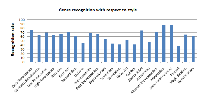
One may note that better performance is achieved for older styles, from the early beginning of artistic painting (as we understand it today) to Post-Impressionism; these styles have a clear representation without too much abstraction. These results are in concordance with previous object detection in paintings (Crowley & Zisserman, 2016), where good performance is achieved for paintings depicting scenes in a rather classical and realistic manner. Also, we achieve good performance for modern styles where the subject is rather unique; in cases such as Minimalism, Abstract Art or Color Field Painting the genre is in fact the style.

In contrast, for styles such as Surrealism, Naive Art, Cubism, Pop Art, the degree of abstraction is high and the CNN has difficulties in interpreting the scene; the scene subject is also variable. Based on this observation, coupled with the observation that in many cases modern paintings reinterpret classical compositions under the rules of new styles, we attempted to create new pseudo-paintings by using a realistic depiction of an old content and a modern style; this is the reason while we tried to neurally transfer abstract styles on older paintings content. Furthermore, this idea is in the same line with neural transfer methods (Gatys et al., 2016; Johnson et al., 2016; Ulyanov et al., 2016; Huang & Belongie, 2017), where almost every time, the reference image had an abstract style, while content that easily comprehensible.

6.3 Domain transfer

The domain transfer experiments were performed iteratively, starting from small sets to larger ones. The motivation lies in the fact that producing relevant images for transfer requires non-negligible effort. We recall that we annotated $\sim 20,000$ artistic photos and we produced more that $30,000$ neurally adapted images.

Each iteration assumes $N$ ($N=250,500\dots$) maximum images in each of the 26 classes; on some classes, since they have too few examples, even in the first iteration this maximum is too generous from the begining. For a detailed number of images existing in each class, we kindly ask the reader to look into Table 1 and to keep in mind that 80% is used for training while 20% is for testing. For iterations corresponding to given $N=250,\dots,10000$, we have added, in all domain transfer scenarios, images from three classes, as follows: cityscape – 2903, landscape – 4467, portrait – 4002. At the end, we have added all images from all classes and all the images available in alternative, transferable, domains.

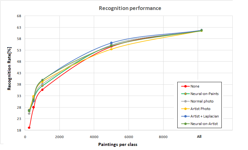
The obtained results may be numerically followed in Table 4, while visually in Figure 5. The baseline performance, where no domain transfer is involved, is on the row marked with “None”. The “Best-improvement” row marks the difference between the best achieving solution and the baseline. “Added image ratio” row represents the ratio between the number of added images and the number of paintings used in this training. Each cell from the column marked with “Avg. improv.” (average improvement) indicates the mean of the improvement for the transfer method.

Table 4: Recognition rates[%] when adding images from “Cityscape”, “Portrait”, “Landscape” to the paintings. At each iteration we keep only the nominated value (250, 500, etc.) from each of the 26 classes. We add the non-paintings from the three classes originating in some domain or adapted with some function. On each column (testing scenario) we marked with bold letters the best performance. Row “None“ indicates the performance when no transfer was performed and thus gives the baseline. “Best-improvement” shows the difference, per column, between the best performance and baseline. “Added image ratio” indicates the percentage of images added to the baseline. Column “Avg. improv.” is the improvement of a transfer scenario with respect to baseline.

Method	Recognition rates [%] when paintings per class					Avg.
	250	500	1000	5000	All	Improv.
None	19.12	27.95	35.66	54.61	61.64	0
Normal Photos (SUN/LFW)	25.28	32.04	38.21	55.31	61.67	2.71
Artist Photos	26.72	32.75	39.27	53.49	61.55	2.96
Laplacian-on-Artist	26.56	30.73	39.84	56.17	61.73	3.21
Neural-on-Paints	26.76	31.98	37.4	55.33	61.47	2.79
Neural-on-Artist	26.33	31.27	39.94	54.88	61.62	3.01
Best-improvement	7.64	4.8	4.18	1.56	0.09	–
Added image ratio[%]	190.04	103.38	58.98	27.33	$\sim$26	–

One should note that improvement (larger than stochastic margin) is achieved only when the number of added images is with at least 30% larger than the number of paintings in the training database and the number of paintings is not too large. Looking at the trends from the last two rows, one may estimate that in order to achieve some $5-10\%$ increase for the entire database, one will need about 3 times the number of paintings to be obtained from some other source, while the same procedure is assumed.

Another visible trend is that original paintings are better that any transferred and adapted image from other domain. We explain this behavior by the content originality of the paintings: artistic works should be considerably different in at least one aspect (e.g. content, local style, composition, subject, etc.) from its predecessors, as to be acknowledged as art. This produces a naturally sparse domain representation for paintings. The sparsity is not easily filled up by knowledge transfer from a similar representation.

At last, the performance of any domain transfer method is not too different from any other. Although by looking at overall improvement, the Laplacian style transfer on artistic photos, is marginally better, the difference is too small (especially given the stochastic margin) that one cannot conclude about a clear winner. This results is somehow surprising, as the highly praised neural style transfer (which produces visually pleasant images) does not show better performance than the Laplacian transfer or than the images themselves.

When comparing the normal photos with artistic photos, the artistic content and the way this content is represented, gives slightly better results. Yet a CNN learns too little from older artistic content to deal with new one.

When comparing the Laplacian transfer with the Neural style transfer, as introduced by Gatys et al. 2016, the significant better representation (larger depth of the feature map) and the better fitting of the latter achieves nothing. At the end of this analysis, we must note that, although claimed, none of these methods implements a “style transfer”, where “style” has the meaning under which is used in art. Although this result has a negative connotation in the sense that expected hypothesis (“style transfer methods does not transfer styles“) does not hold, we feel that we should make it public, especially given the recent argumentation by Borji 2018. Furthermore, we see that has a strong positive connotation too: it shows that it is much easier to improve the performance of the CNN when dealing with understanding art by simply showing it very large quantities of relevant photographs.

Figure 5: The genre recognition rate with respect to transferred images per class, as a function of the augmentation method. When the number of transferred images dominate over the number of painting in the database, the performance improves

7 Discussion and Conclusions

In this paper we discussed the CNN capabilities to recognize the scene (genre) in a painting. The first contribution is that we clearly showed that machine learning systems (deep CNNs) are confused by the abstraction level from art. The experiment with abstract art showed that they cannot easily generalize with respect to style and that, the more abstract a style is, the lower is the recognition rate of the genre (painting subject). In this sense, the CNN is similar with humans, who also find the abstract representations of scenes to be more puzzling.

The secondary set of contributions results from the experimentation with domain transfer as an alternative to increase the overall performance and we have found that: (1) limited improvement is easily doable when the training set of paintings is small; (2) methods claiming to transfer style, either Laplacian based, either neural based, although produce visually very pleasant and intriguing images, are ineffective as domain adaptation methods with respect to style. One possible explanation is that “style” as understood by the transfer methods is not the same with “artistic style” in the sense of art movement.

Lastly, the third contribution is related to understanding the structure of the paintings domain. Due to the necessary criteria for some work to be accepted as a work of art, which implies significant artistic novelty with respect to its predecessors, the paintings domain is more sparse than that of the normal images. Given the problem to improve the performance, a CNN learns to better deal with some new work of art, when more works of art are presented to it in the training set. The CNNs are similar to humans in this behavior as well, as art expert do not learn their job looking at normal images.

8 Acknowledgment

The work was supported by grants of the Romanian National Authority for Scientific Research and Innovation, CNCS UEFISCDI, number PN-II-RU-TE-2014-4-0733 and respectively, CCCDI-UEFISCDI, project number 96BM. The authors would like to thank NVIDIA Corporation for donating the Tesla K40c GPU that helped run the experimental setup for this research.

References

- Agarwal et al. (2015) Agarwal, S., Karnick, H., Pant, N., and Patel, U. Genre and style based painting classification. In IEEE Winter Conference on Applications of Computer Vision, pp. 588–594, 2015.
- Aubry et al. (2013) Aubry, M., Russell, B., and Sivic, J. Painting-to-3d model alignment via discriminative visual elements. ACM Transactions of Graphics, 33(2), 2013.
- Aubry et al. (2014) Aubry, M., Paris, Sylvain, Hasinoff, Samuel W., Kautz, Jan, and Durand, Fredo. Fast local laplacian filters: Theory and applications. ACM Transactions of Graphics, 33(5), 2014.
- Badea et al. (2017) Badea, Mihai, Florea, Corneliu, Florea, Laura, and Vertan, Constantin. Efficient domain adaptation for painting theme recognition. In Signals, Circuits and Systems (ISSCS), 2017 International Symposium on, pp. 1–4, 2017.
- Bae et al. (2006) Bae, Soonmin, Paris, Sylvain, and Durand, Frédo. Two-scale tone management for photographic look. In ACM Transactions on Graphics, volume 25, pp. 637–645, 2006.
- Bar et al. (2014) Bar, Y., Levy, N., and Wolf, L. Classification of artistic styles using binarized features derived from a deep neural network. In European Conference on Computer Vision Workshops - Visart, pp. 71–84, 2014.
- Ben-David et al. (2010) Ben-David, Shai, Blitzer, John, Crammer, Koby, Kulesza, Alex, Pereira, Fernando, and Wortman Vaughan, Jennifer. A theory of learning from different domains. Machine Learning Journal, 79(1-2):1–2, 2010.
- Bentkowska-Kafel & Coddington (2010) Bentkowska-Kafel, A. and Coddington, J. Computer vision and image analysis of art. In SPIE, 2010.
- Borji (2018) Borji, Ali. Negative results in computer vision: A perspective. Image and Vision Computing, 69:1 – 8, 2018.
- Cai et al. (2015) Cai, H., Wu, Q., and Hall, P. Beyond photo-domain object recognition: Benchmarks for the cross-depiction problem. In International Conference on Computer Vision workshops - TASK, pp. 262–273, 2015.
- Chen & Schmidt (2016) Chen, Tian Qi and Schmidt, Mark. Fast patch-based style transfer of arbitrary style. CoRR, abs/1612.04337, 2016.
- Cichy et al. (2016) Cichy, R.M., Khosla, Aditya, Pantazis, Dimitrios, Torralba, Antonio, and Oliva, Aude. Comparison of deep neural networks to spatio-temporal cortical dynamics of human visual object recognition reveals hierarchical correspondence. Scientific Reports, 6, 2016.
- Condorovici et al. (2013) Condorovici, R., Florea, C., and Vertan, C. Painting scene recognition using homogenous shapes. In Advanced Concepts for Intelligent Vision Systems, pp. 262–273, 2013.
- Crowley & Zisserman (2016) Crowley, Elliot J and Zisserman, Andrew. The art of detection. In European Conference on Computer Vision, pp. 721–737, 2016.
- Dalal & Triggs (2005) Dalal, N. and Triggs, B. Histograms of oriented gradients for human detection. In IEEE Conference on Computer Vision and Pattern Recognition, pp. 886–893, 2005.
- DiCarlo et al. (2012) DiCarlo, J.J., Zoccolan, D., and Rust, N.C. How does the brain solve visual object recognition? Neuron, 73(3):415–434, 2012.
- Dollár et al. (2014) Dollár, Piotr, Appel, Ron, Belongie, Serge, and Perona, Pietro. Fast feature pyramids for object detection. IEEE Transactions on Pattern Analysis and Machine Intelligence, 36(8):1532–1545, 2014.
- Donahue et al. (2014) Donahue, Jeff, Jia, Yangqing, Vinyals, Oriol, Hoffman, Judy, Zhang, Ning, Tzeng, Eric, and Darrell, Trevor. Decaf: A deep convolutional activation feature for generic visual recognition. In International Conference on Machine Learning, pp. 647–655, 2014.
- Fischer et al. (2014) Fischer, Philipp, Dosovitskiy, Alexey, and Brox, Thomas. Descriptor matching with convolutional neural networks: a comparison to sift. arXiv preprint arXiv:1405.5769, 2014.
- Florea et al. (2017a) Florea, Corneliu, Badea, Mihai, Florea, Laura, and Vertan, Constantin. Domain transfer for delving into deep networks capacity to de-abstract art. In Scandinavian Conference on Image Analysis, pp. 337–349, 2017a.
- Florea et al. (2017b) Florea, Corneliu, Toca, Cosmin, and Gieseke, Fabian. Artistic movement recognition by boosted fusion of color structure and topographic description. In IEEE Winter Conference on Applications of Computer Vision, pp. 569–577, 2017b.
- Gatys et al. (2016) Gatys, Leon A, Ecker, Alexander S, and Bethge, Matthias. Image style transfer using convolutional neural networks. In IEEE Conference on Computer Vision and Pattern Recognition, pp. 2414–2423, 2016.
- Gretton et al. (2012) Gretton, Arthur, Borgwardt, Karsten M, Rasch, Malte J, Schölkopf, Bernhard, and Smola, Alexander. A kernel two-sample test. Journal of Machine Learning Research, 13(Mar):723–773, 2012.
- Hall et al. (2015) Hall, P., Cai, H., Wu, Q., and Corradi, T. Cross-depiction problem: Recognition and synthesis of photographs and artwork. Computational Visual Media, 1(2):91–103, 2015.
- He et al. (2016) He, Kaiming, Zhang, Xiangyu, Ren, Shaoqing, and Sun, Jian. Deep residual learning for image recognition. In IEEE Conference on Computer Vision and Pattern Recognition, pp. 770–778, 2016.
- Herranz et al. (2016) Herranz, Luis, Jiang, Shuqiang, and Li, Xiangyang. Scene recognition with cnns: objects, scales and dataset bias. In IEEE Conference on Computer Vision and Pattern Recognition, pp. 571–579, 2016.
- Hinton et al. (2015) Hinton, Geoffrey, Vinyals, Oriol, and Dean, Jeff. Distilling the knowledge in a neural network. arXiv:1503.02531, 2015.
- Huang et al. (2007) Huang, Gary B., Jain, Vidit, and Learned-Miller, Erik. Unsupervised joint alignment of complex images. In International Conference on Computer Vision, 2007.
- Huang & Belongie (2017) Huang, Xun and Belongie, Serge. Arbitrary style transfer in real-time with adaptive instance normalization. In International Conference on Computer Vision, pp. 1501–1510, 2017.
- Johnson et al. (2016) Johnson, Justin, Alahi, Alexandre, and Fei-Fei, Li. Perceptual losses for real-time style transfer and super-resolution. In European Conference on Computer Vision, pp. 694–711, 2016.
- Karayev et al. (2014) Karayev, S., Trentacoste, M., Han, H., Agarwala, A., Darrell, T., Hertzmann, A., and Winnemoeller, H. Recognizing image style. In British Machine Vision Conference, 2014.
- Krizhevsky et al. (2012) Krizhevsky, Alex, Sutskever, Ilya, and Hinton, Geoffrey E. Imagenet classification with deep convolutional neural networks. In Pereira, F., Burges, C. J. C., Bottou, L., and Weinberger, K. Q. (eds.), Advances in Neural Information Processing Systems, pp. 1097–1105, 2012.
- Li et al. (2017) Li, Yanghao, Wang, Naiyan, Liu, Jiaying, and Hou, Xiaodi. Demystifying neural style transfer. In Proceedings of International Joint Conference on Artificial Intelligence, pp. 2230–2236, 2017.
- Lu et al. (2015) Lu, Jie, Behbood, Vahid, Hao, Peng, Zuo, Hua, Xue, Shan, and Zhang, Guangquan. Transfer learning using computational intelligence: A survey. Knowledge-Based Systems, 80:14 – 23, 2015.
- Monroy et al. (2014) Monroy, Antonio, Bell, Peter, and Ommer, Bjorn. Morphological analysis for investigating artistic images. Image and Vision Computing, 32(6):414 – 423, 2014.
- Ojala et al. (2002) Ojala, T., Pietikäinen, M., and Mäenpää, T. Multiresolution gray-scale and rotation invariant texture classification with local binary patterns. IEEE Transactions on Pattern Analysis and Machine Inteligence, 24(7):971–987, 2002.
- Reinhard et al. (2001) Reinhard, E., Ashikhmin, M., Gooch, B., and Shirley, P. Color transfer between images. IEEE Computer Graphics and Applications, 21(5):34–41, 2001.
- Saenko et al. (2010) Saenko, Kate, Kulis, Brian, Fritz, Mario, and Darrell, Trevor. Adapting visual category models to new domains. In European Conference on Computer Vision, pp. 213–226, 2010.
- Saleh & Elgammal (2015) Saleh, Babak and Elgammal, Ahmed. Large-scale classification of fine-art paintings: Learning the right metric on the right feature. In International Conference on Data Mining Workshops. IEEE, 2015.
- Sewards (2011) Sewards, Terence V. Neural structures and mechanisms involved in scene recognition: A review and interpretation. Neuropsychologia, 49(3):277 – 298, 2011.
- Simonyan & Zisserman (2015) Simonyan, K. and Zisserman, A. Very deep convolutional networks for large-scale image recognition. In International Conference on Learning Representations, 2015.
- Sunkavalli et al. (2010) Sunkavalli, Kalyan, Johnson, Micah K, Matusik, Wojciech, and Pfister, Hanspeter. Multi-scale image harmonization. In ACM Transactions on Graphics, volume 29, pp. 125, 2010.
- Tan et al. (2016) Tan, Wei Ren, Chan, Chee Seng, Aguirre, Hernan E., and Tanaka, Kiyoshi. Ceci n est pas une pipe: A deep convolutional network for fine-art paintings classification. In IEEE Internation Conference on Image Processing, 2016.
- Thomas & Kovashka (2016) Thomas, Christopher and Kovashka, Adriana. Seeing behind the camera: Identifying the authorship of a photograph. In IEEE Conference on Computer Vision and Pattern Recognition, pp. 3494–3502, 2016.
- Ulyanov et al. (2016) Ulyanov, Dmitry, Lebedev, Vadim, Vedaldi, Andrea, and Lempitsky, Victor. Texture networks: feed-forward synthesis of textures and stylized images. In International Conference on Machine Learning, pp. 1349–1357, 2016.
- Vedaldi & Fulkerson (2010) Vedaldi, A. and Fulkerson, B. Vlfeat: An open and portable library of computer vision algorithms. In Proceedings of ACM International Conference on Multimedia, pp. 1469–1472, 2010.
- Xiao et al. (2010) Xiao, Jianxiong, Hays, James, Ehinger, Krista A, Oliva, Aude, and Torralba, Antonio. Sun database: Large-scale scene recognition from abbey to zoo. In IEEE Conference on Computer Vision and Pattern Recognition, pp. 3485–3492, 2010.
- Zeiler & Fergus (2014) Zeiler, Matthew D and Fergus, Rob. Visualizing and understanding convolutional networks. In European Conference on Computer Vision, pp. 818–833, 2014.
- Zhou et al. (2014) Zhou, Bolei, Lapedriza, Agata, Xiao, Jianxiong, Torralba, Antonio, and Oliva, Aude. Learning deep features for scene recognition using places database. In Neural Information Processing Systems, 2014.
- Zhou et al. (2015) Zhou, Bolei, Khosla, Aditya, Lapedriza, Agata, Oliva, Aude, and Torralba, Antonio. Object detectors emerge in deep scene cnns. In Internation Conference on Learning Representations, 2015.