Keywords:

.

state-dependence of interactions;

effective Hamiltonians;

logarithmic nonlinearities;

linearized quantum toy model;

PACS number:

.

PACS 03.65.Ge Solutions of wave equations: bound states

Abstract

Singular repulsive barrier $V(x)=-g\ln(|x|)$ inside a square well is interpreted and studied as a linear analogue of the state-dependent interaction ${\cal L}_{eff}(x)=-g\,\ln[\psi^{*}(x)\psi(x)]$ in nonlinear Schrödinger equation. In the linearized case, Rayleigh-Schrödinger perturbation theory is shown to provide a closed-form spectrum at the sufficiently small $g$ or after an amendment of the unperturbed Hamiltonian. At any spike-strength $g$, the model remains solvable numerically, by the matching of wave functions. Analytically, the singularity is shown regularized via the change of variables $x=\exp y\$ which interchanges the roles of the asymptotic and central boundary conditions.

1 Motivation

The study of complicated quantum systems may be facilitated by a judicious, less explicit treatment of certain less essential degrees of freedom [1]. The reduction may lead to simplifications which are often achieved via a tentative replacement of the exact, full-Hilbert-space linear Schrödinger equation

$${\rm i}\partial_{t}\,|\Psi\rangle=\mathfrak{H}\,|\Psi\rangle$$ (1)

by its reduced, open-subsystem version. In this manner a remarkably successful description of the physical reality has been achieved, in multiple phenomenological applications (cf., e.g., their compact review in paper I [2]) via nonlinear evolution equations in which the effective-interaction potential was admitted state-dependent,

$${\rm i}\partial_{t}\psi({x},t)=\left[-\partial_{x}^{2}+V_{(eff)}({x},t)\right]\,\psi({x},t)\,,\ \ \ \ \ \ \ \ V_{(eff)}({x},t)=V[\psi({x},t),x,t]$$ (2)

and, in particular, in which the nonlinearity has been chosen logarithmic,

$$V[\psi({x},t),x,t]=-g\,\ln[\psi^{*}(x,t)\psi(x,t)]\,,\ \ \ \ g>0\,.$$ (3)

In paper I it has been argued that an important formal support of the latter choice may be seen in its asymptotic system-confinement self-consistency. Indeed, one can easily verify that the insertion of a tentative, exactly solvable harmonic-oscillator potential $V_{(HO)}(x)=x^{2}$ in Eq. (2) would yield the wave functions in closed form

$$\psi_{(HO)}({x},t)\sim\exp(-iE_{(HO)}t)\,\exp\left(-{x}^{2}/2+{\cal O}(\ln|{x}|)\right)\,,\ \ \ \ \ \ \ \ |x|\gg 1\,.$$ (4)

In turn, expression (3) will lead to the qualitatively correct asymptotics

$$-\ln[\psi^{*}_{(HO)}({x},t)\psi_{(HO)}({x},t)]={x}^{2}+{\cal O}(\ln{|{x}|})\,,\ \ \ \ \ \ \ \ |x|\gg 1\,$$ (5)

of the confining potential.

In the constructive part of paper I it has been recalled and demonstrated that certain node-less, “gausson” solutions of the evolution Eq. (2) may be well-behaved at all times $t$. The existence of the “gaussons” can be viewed as a consequence of the absence of the nodal zeros in the initial (i.e., say, $t=0$) choice of the ground-state-like wave function $\psi(x,0)$. In other words, what remained unclarified in paper I was the question of the properties of all of the non-gausson solutions of Eq. (2) + (3). Presumably, most of these non-gausson solutions might be based on the anomalous initial wave functions $\psi_{N}(x,0)$ having an $N-$plet of the excited-state-like nodal zeros at some $N\geq 1$.

Naturally, this would make the nonlinear interaction term (3) singular. Locally (i.e., out of the asymptotic region and near any nodal zero $x_{j}$ with $1\leq j\leq N$) this follows from the simple-zero estimate

$$\psi_{N}(x,0)\sim x-x_{j}\,.$$ (6)

In the first nontrivial non-gausson case we may choose $N=1$ and require $x_{1}=0$ (i.e., an initial-time antisymmetry of the wave function). In the light of the above-mentioned HO example one expects that, with certain implicit, not too well tractable error terms, we should work with potentials of the form

$$V_{(eff)}({x},0)\ \sim\ x^{2}-2g\ln|x|+\ldots\,$$ (7)

or, in an alternative, technically simpler confining square-well (SW) approximation, with

$$V_{(eff)}({x},0)\ \sim\ V_{(SW)}({x})=\left\{\begin{array}[]{cl}\infty\,,&|x|\geq 1\,,\\ -2g\ln|x|\,,&|x|<1\,.\end{array}\right.$$ (8)

In what follows we intend to complement the global non-linear-theory considerations of paper I by the missing and relevant discussion of some of the technical consequences of the emergence of the logarithmic singularity at one or more nodal points $x_{j}$ and, first of all, of certain properties of the bound states in the first nontrivial excitation-simulating linear interaction potential (8).

2 Weak-coupling regime

The enormous simplicity of the one-dimensional quantum square well oscillator makes it suitable for pedagogical purposes. Its analyses appear not only in conventional textbooks [3, 4] but also in the less conventional studies of supersymmetric quantum systems [5, 6]. The elementary nature of the square-well model found also nontrivial applications in parity times time-reversal symmetric quantum mechanics [7, 8, 9, 10] or in certain sophisticated versions of perturbation theory [11].

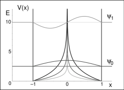
Figure 1: The shapes of the perturbed square-well potentials (8) at $g=1/4$ (the lowest, light spike), $g=1/2$ (the intermediate spike) and $g=1$ (the upper spike). Horizontal lines mark the first two energy levels for $g=0$. Attached to them, the picture also displays the shapes of the unperturbed wave functions.

We intend to analyze the interaction in its special form (2) + (8), i.e., in the first nontrivial $N=1$ special case. Thus, our attention gets shifted to the linearized model represented by the conventional and time-independent ordinary differential Schrödinger equation for quantum stationary bound states,

$$-\,\frac{{\rm d}^{2}}{{\rm d}x^{2}}\,\psi_{n}(x)-2g\,\ln(|x|)\,\psi_{n}(x)=E_{n}\,\psi_{n}(x)\,,\ \ \ \ \ \ \psi_{n}(\pm 1)=0\,,\ \ \ \ n=0,1,\ldots\,.$$ (9)

The spike-shaped logarithmic barrier is unbounded, repulsive and centrally symmetric here - cf. Fig. 1 where the shape of the potential is displayed at $g=0.25,0.5$ and $1$.

It is worth adding that although we are choosing here (i.e., in Eq. (6)) the first nontrivial nodal number $N=1$ for the sake of simplicity, Eq. (9) describes all of the bound states generated by the linearized toy-model interaction (8). These states are numbered by a different, lower-case index $n$. Naturally, one would have to set, for the sake of consistency, $n=N$ at the end of the analysis and, in principle at least, before an ultimate return to the initial nonlinear-equation setting.

2.1 First-order approximation

At the small but non-vanishing strengths $g>0$ our central barrier is infinitely high so that one might suspect that it is impenetrable. The expectation is wrong. In the Rayleigh-Schrödinger perturbation-expansion series arrangement [12] with

$$E_{n}=E_{n}(g)=E_{n}^{[0]}+g\,E_{n}^{[1]}+g^{2}\,E_{n}^{[2]}+\ldots\,,\ \ \ \ \ \ E_{n}^{[0]}=[(n+1)\pi/2]^{2}\,,\ \ \ \ n=0,1,\ldots$$ (10)

the first-order shifts

$$E_{2p}^{[1]}\sim-4\,\int_{0}^{1}\cos^{2}[(2p+1)\pi\,x/2]\,\ln(|x|)\,dx\,,\ \ \ \ \ \ p=0,1,\ldots$$ (11)

and

$$E_{2q+1}^{[1]}\sim-4\,\int_{0}^{1}\sin^{2}[(q+1)\pi\,x]\,\ln(|x|)\,dx\,,\ \ \ \ \ \ q=0,1,\ldots$$ (12)

of the spectrum of our conventional perturbed square well are, obviously, positive and finite.

One can easily prove that the latter corrections are all finite, indeed. The proof may be based on the fact that all of the integrands are bounded on the subintervals of $x\in(\epsilon,1)$ with any $\epsilon=\exp(-R)\in(0,1)$ (i.e., any $R>0$). Thus, it is sufficient to find a bound for the integrals over a short interval of $x\in(0,\epsilon)$. With a sufficiently large $R\gg 1$ we obtain an explicit estimate

$$-4\,\int_{0}^{\epsilon}\sin^{2}[(q+1)\pi\,x]\,\ln(|x|)\,dx\sim\int_{0}^{\epsilon}\,x^{2}\,\ln(|x|)\,dx=\int_{-\infty}^{-R}\,y\,e^{3y}\,dy=-\frac{1}{9}(3R+1)\,e^{-3R}\,$$ (13)

showing that the odd-state integrals are all exponentially small. In the even-state case we have, similarly, the estimate

$$-4\,\int_{0}^{\epsilon}\cos^{2}[(2p+1)\pi\,x/2]\,\ln(|x|)\,dx\sim\int_{0}^{\epsilon}\,\ln(|x|)\,dx=\int_{-\infty}^{-R}\,y\,e^{y}\,dy=-(R+1)\,e^{-R}\,$$ (14)

leading to the same ultimate finite-correction conclusion.

2.2 Closed formulae

The even-state contribution seems larger than the odd-state contribution, for the sufficiently large $R$ at least. For a more reliable, $R-$independent comparison of the corrections $E_{n}^{[1]}$ at the even and odd $n$ it is necessary to introduce the conventional sine-integral special functions $Si(x)=\int_{0}^{x}\,\sin(t)/t\,dt\$ and to evaluate the first-order corrections exactly. Fortunately, this is feasible yielding the following formulae,

$$E_{2p}^{[1]}=2+\frac{2}{(2p+1)\pi}\,Si[(2p+1)\pi]\,,\ \ \ \ p=0,1,\ldots\,,$$ (15)

$$E_{2q+1}^{[1]}=2-\frac{2}{(2q+2)\pi}\,Si[(2q+2)\pi]\,,\ \ \ \ q=0,1,\ldots\,.$$ (16)

Table 1: The first ten numerical coefficients $E_{n}^{[1]}$ in Eq. (10).

$n$	symmetric $\psi_{n}(x)$	antisymmetric $\psi_{n}(x)$
0	3.178979744
1		1.548588333
2	2.355395491
3		1.762515165
4	2.208042866
5		1.838931594
6	2.146975999
7		1.878156443
8	2.113606700
9		1.902022366

The evaluation of the numerical values of the special functions $Si(x)$ is routine and yields the first-order perturbation-series coefficients as sampled in Table 1. The inspection of the Table reveals that the energy shifts at the even quantum numbers $n=2p$ will be always larger than the partner shifts at the odd quantum numbers $n=2p+1$. In other words, even the present “soft”, logarithmic shape of the central repulsive barrier will lead to the quasi-degeneracy pattern in the spectrum of the logarithmically spiked bound states.

2.3 Limitations of applicability

By the logarithmically singular but still positive-definite barrier the unperturbed spectrum is being pushed upwards. Still, due to the immanent weakness of the singularity of the logarithmic type even in the strong-coupling dynamical regime with $g\gg 1$, the expected effect of the quasi-degeneracy will get quickly suppressed with the growth of $n$, i.e., of the excitation. In contrast to the stronger and more common (e.g., power-law) models of the repulsion in the origin, this will make the real influence of the logarithmic barrier restricted to the low-lying spectrum.

Fig. 2 may be recalled for an explicit quantitative illustration of the latter expectation. Using just the most elementary leading-order-approximation estimates we see there that while the prediction of the quasi-degeneracy between the ground (i.e., $n=0$) and the first excited (i.e., $n=1$) state might still occur near the reasonably small value of coupling $g_{0,1}^{[1]}=4.540138798$, the next analogous crossing of the first-order energies $E_{2}^{[1]}$ and $E_{3}^{[1]}$ only takes place near the estimate as large as $g_{2,3}^{[1]}=29.13203044$, etc.

Figure 2: The coupling-dependence of the low-lying spectrum in the Rayleigh-Schrödinger first order (i.e., linear-extrapolation) approximation.

The same Fig. 2 also shows that another first-order crossing may be detected for $E_{0}^{[1]}$ and $E_{2}^{[1]}$, emerging even earlier (i.e., at $g_{0,2}^{[1]}=23.96744320$) and being, obviously, spurious. In other words, for the prediction of the quasidegeneracy in the strong-coupling dynamical regime the knowledge of the mere first-order perturbation corrections must be declared insufficient.

3 Strong-coupling regime

Beyond the domain of applicability of the weak-coupling perturbation theory, alternative (mainly, purely numerical) methods must be used in order to determine the spectrum of bound states of our linearized toy model exactly, i.e., with arbitrary prescribed precision.

As long as these bound states are determined by the ordinary differential Schrödinger Eq. (9), there exists a number of methods of their construction. The choice of the method may be inspired by the inspection of Figs. 1 and 2. This indicates that the influence of our singular logarithmic potential (8) is felt, first of all, by the low-lying bound states and/or in the strong-coupling regime. Directly, this may be demonstrated by the routine numerical construction of the wavefunctions (sampled in Fig. 3) and by the routine numerical evaluation of the energies (sampled in Table 2). In both cases, due attention must be paid to the singular nature of our potential (8) in the origin. This is a challenging aspect of the numerical calculations which will be discussed and illustrated by some examples in what follows.

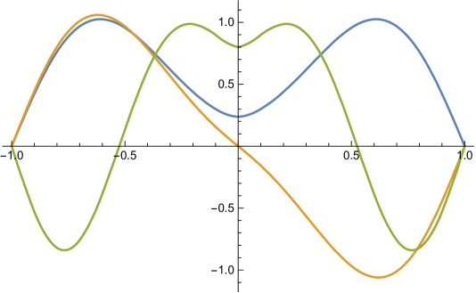
Figure 3: The first three wavefunctions at $g=10$.

Table 2: Numerically determined low-lying spectrum.

$g$	$E_{0}$	$E_{1}$	$E_{2}$	$E_{3}$	$E_{4}$
0.00	2.4674	9.8696	22.207	39.478	61.685
0.25	3.2478	10.255	22.796	39.928	62.265
0.50	4.0097	10.638	23.394	40.369	62.817
1.00	5.4784	11.395	24.618	41.252	63.931

3.1 Mathematical challenge: singularity

Without any real loss of generality our attention may stay restricted to the characteristic $N=1$ model (9). This model is sufficiently general when treated as a system of two (viz., $x<0$ and $x>0$) linear differential equations for which the logarithmic derivatives of the respective wave functions have to be matched in the origin, i.e., at $x_{1}=0$. In this sense, naturally, the generalization to the $N>1$ cases would be straightforward.

Once we fix $N=1$ we may split the original linear differential equation into a pair living on the two respective half-intervals, viz.,

$$-\,\frac{{\rm d}^{2}}{{\rm d}x_{(L)}^{2}}\,\psi_{n}(x_{(L)})-2g\,\ln(-x_{(L)})\,\psi_{n}(x_{(L)})=E_{n}\,\psi_{n}(x_{(L)})\,,\ \ \ \ \ \ x_{(L)}\in(-1,0)\,$$ (17)

and

$$-\,\frac{{\rm d}^{2}}{{\rm d}x_{(R)}^{2}}\,\psi_{n}(x_{(R)})-2g\,\ln(x_{(R)})\,\psi_{n}(x_{(R)})=E_{n}\,\psi_{n}(x_{(R)})\,,\ \ \ \ \ \ x_{(R)}\in(0,1)\,.$$ (18)

As long as the bound-state solutions have a definite parity at $N=1$, one of these equations may be omitted as redundant.

3.2 Amended zero-order approximation

Due to the symmetry of our potential it will be sufficient to consider just Eq. (17) on the negative finite half-interval. The correct matching with Eq. (18) may be then guaranteed by means of the pair of ad hoc  boundary conditions in the origin,

$$\left\{\begin{array}[]{ll}\psi_{n}(0)\neq 0\,,\ \ \psi_{n}^{\prime}(0)=0\,,&{\rm(even\ states)}\,,\\ \psi_{n}(0)=0\,,\ \ \psi_{n}^{\prime}(0)\neq 0\,,&{\rm(odd\ states)}\,.\\ \end{array}\right.\,$$ (19)

The application of recipe (19) must be performed with due care. The reason lies in the unbounded, singular nature of our logarithmic potential in the origin. Fortunately, the necessary deeper analysis of the matching conditions at $x=0$ might be also complemented by an amendment of the perturbation-theory considerations of section 2.

Inside a suitable small interval of $x\in(-d,d)$ with $d<1$ we may contemplate an approximative replacement of the logarithmic repulsive spike $V(x)$ by a rectangular barrier of a finite height $\kappa_{0}^{2}=E+\kappa^{2}$. At any given/tentative energy $E$ we may demand that $E=k^{2}=-2g\ln d$, i.e., that $d=d(E)=\exp[-E/(2g)]$. This will weaken our potential $V()x)$ to the left from $x=-d$ while strengthening it, locally at least, to the right from $x=-d$. The approximate wavefunctions may be then written down in the following closed elementary-function form

$$\psi(x)\approx\left\{\begin{array}[]{lll}\sin[(x+1)k]\,,&x\in(-1,-d)\,,&\\ \sin[(x-1)k]\,,&x\in(d,1)\,,&\\ {\rm cosh}[\kappa x]\,,&x\in(-d,d)&{\rm(even\ states)}\,,\\ {\rm sinh}[\kappa x]\,,&x\in(-d,d)&{\rm(odd\ states)}\,.\\ \end{array}\right.\,$$ (20)

Its components must be properly matched at $x=\pm d=\pm d(E)$ and, if needed, also properly normalized. It is, perhaps, worth adding that inside the interval of $E\in(5,5.5)$ (i.e., in the vicinity of the gound-state energy, cf. Table 2), the decrease of the value of $d(E)$ from $d(5)\approx 0.08208499862$ to $d(5.5)\approx 0.06392786121$ is almost linear, i.e., comparatively easily kept under control in the calculations. This means that the $d-$dependence of our approximative rectangular barrier may be also re-interpreted as its energy-dependence.

3.3 Regularized Schrödinger equation

The remarkable technical challenge is that the point of the matching of the wavefunctions coincides with the singularity of the potential. In the literature, similar situation is usually encountered in connection with the Coulombic repulsion $\sim 1/x$ [13, 14]. Here, the repulsion is much weaker but the regularization of the model is still by far not routine. In the analytic-function-theory language it can rely upon the change of variables

$$x_{(L)}=-\exp(-\lambda)\,,\ \ \ \ \ \ \ x_{(R)}=\exp(\rho)\,,$$ (21)

and

$$\psi_{n}(x_{(L)})=\exp(-\lambda/2)\,\phi^{(-)}(\lambda)\,,\ \ \ \ \ \ \ \psi_{n}(x_{(R)})=\exp(\rho/2)\,\phi^{(+)}(\rho)\,.$$ (22)

In the left subinterval of $x_{(L)}\in(-1,0)$ this yields the initial-value problem

$$-\,\frac{{\rm d}^{2}}{{\rm d}\lambda^{2}}\,\phi(\lambda)+\frac{1}{4}\,\phi(\lambda)=\exp(-2\lambda)\,\left[E-2g\lambda\right]\,\phi(\lambda),\ \ \ \ \phi(0)=0\,,\ \ \ \ \phi^{\prime}(0)=1\,$$ (23)

on the half-line of $\lambda\in(0,\infty)$.

We see that the singularity has been moved to infinity. Thus, after the change of variables (22), the wavefunction-matching relations (19) may purely formally be replaced by their appropriate asymptotic analogues supplementing Eq. (23). In fact, we shall show below that this is really a purely analytic idea, not leading to any practical numerical advantages.

Analogously, the second half of our initial differential equation with $x_{(R)}\in(0,1)$ is converted into equivalent second half-line version

$$-\,\frac{{\rm d}^{2}}{{\rm d}\rho^{2}}\,\phi(\rho)+\frac{1}{4}\,\phi(\rho)=\exp(2\rho)\,\left[E+2g\rho\right]\,\phi(\rho),\ \ \ \ \phi(0)=0\,,\ \ \ \ \phi^{\prime}(0)=(-1)^{n+1}=\pm 1\,$$ (24)

where $\rho\in(-\infty,0)$. The latter equation is redundant again, obtainable from the former one by the mere change of parity alias  replacement $\rho\to-\lambda$.

4 Numerical solutions

Using our amended approximation (20) we could obtain a qualitatively  correct shape of the wavefunctions, in principle at least. Naturally, the fully reliable construction of bound states must be performed by the controlled-precision numerical integration of our ordinary differential Schrödinger equations. These results were sampled in Fig. 3 above. What is worth emphasizing is that in this setting the singularity of potential $V(x)$ remains tractable by the standard numerical-integration software, say, of MATHEMATICA or MAPLE.

4.1 Qualitative theory: re-parametrized Schrödinger equation

For our model (9), obviously, an extension of applicability of the conventional perturbation theory could have been based on the use of various more sophisticated zero-order shapes of $V_{0}(x)$. In particular, we could obtain a more quickly convergent sequence of perturbation approximations when using the specific rectangular-potential choice of $V_{0}^{(RP)}(x)$ of paragraph 3.2.

One of the other benefits of the amendment would be qualitative, based on the observation that a small deformation of the special potential $V_{0}^{(RP)}(x)$ of paragraph 3.2 must lead just to a small deformation of the related trigonometric definitions (20) of the wavefunctions.

Via these deformations, we may even return exactly to our full-fledged logarithmic potential $V(x)$. Such a return would be achieved by means of the replacement of the effective-momentum constant $k=\sqrt{E}$ by a weakly coordinate-dependent function $\mu(E,x)=\sqrt{E-V(x)}$. The other constant $\kappa=\kappa(E)$ gets replaced by the effective barrier-height $\nu(E,x)=\sqrt{V(x)-E}$. As a result, this enables us to rewrite our Schrödinger equation in the partitioned form

$$-\,\frac{{\rm d}^{2}}{{\rm d}x^{2}}\,\psi(x)=\left\{\begin{array}[]{ll}\ \ \mu^{2}(E,x)\,\psi(x)\,,&x\in(-1,-d)\bigcup(d,1)\,,\\ -\nu^{2}(E,x)\,\psi(x)\,,&x\in(-d,d)\,.\\ \end{array}\right.\,$$ (25)

By construction, this equation is exact. Still, in the light of Eq. (20) it may be assigned the approximate elementary solutions

$$\psi(x)\approx\pm\,\left\{\begin{array}[]{lll}\sin[\mu(E,x)(x+1)]\,,&x\in(-1,-d)\,,&\\ \sin[\mu(E,x)(x-1)]\,,&x\in(d,1)\,,&\\ {\rm cosh}[\nu(E,x)x]\,,&x\in(-d,d)&{\rm(even\ states)}\,,\\ {\rm sinh}[\nu(E,x)x]\,,&x\in(-d,d)&{\rm(odd\ states)}\,.\\ \end{array}\right.\,$$ (26)

Once we take into account the parity, the matching in the origin remains trivial. The decisive role will now be played, instead, by the smoothness (i.e., sort of matching) of the amended approximate wave functions (26) at the energy-dependent point $x=-d<0$ or, equivalently, at $x=d>0$.

4.2 The danger of ill-conditioning

The wavefunction $\psi_{0}(x)=\psi(x)$ is nodeless and spatially symmetric. It must obey the ordinary differential Eq. (17) on half-interval so that its construction may proceed numerically. This yields the $x\to 0^{-}$ limiting values which must be made compatible with the upper line of Eq. (19) via a suitable choice of energy $E$. Such an algorithm the leads to the results sampled by Table 2.

In principle, we could also employ the change of variables (21) and (22) and replace Eq. (17) by its equivalent version (23). This enables us to transfer the central left-right matching (19) of wavefunctions to its analogue in infinity, i.e., in the limit $\lambda\to+\infty$.

The key merit of such an arrangement lies in the clear picture of the analyticity properties and, in particular, in the asymptotic negligibility of the right-hand side of Eq. (23). For this reason the new equation may be immediately assigned the elementary general asymptotic solution

$$\phi(\lambda,E)=const\,e^{\lambda/2+{\rm corrections}}+f(E)e^{-\lambda/2+{\rm corrections}}\,.\ \ \ \ \ \ \lambda\gg 1\,.$$ (27)

The changes of the energy only influence here the subdominant term which is exponentially small. This means that any  numerical solution of the initial-value problem (23) will remain insensitive to the variations of the tentative energy. Hence, the task is ill-conditioned.

Table 3: The failure of the backward-iteration method based on Eqs. (23) and (28). At $q=1$, the convergence of $\phi(0)\to 0$ with respect to $\lambda_{\rm max}\to\infty$ is too slow.

$E$	$\lambda_{\rm max}$	evaluated $\phi(0)$	difference
5.55	3.50	-0.064333935	-
	3.75	-0.059104634	-0.0052
	4.00	-0.053830824	-0.0053
	4.25	-0.048788380	-0.0050
5.45	3.50	-0.037417250	-
	3.75	-0.031754144	-0.0057
	4.00	-0.026113710	-0.0056
	4.25	-0.020763014	-0.0053

One has to try to start the reconstruction in the opposite direction initiated at a sufficiently large $\lambda_{\rm max}\gg 1$ via a suitable tentative choice of the initial values of the wavefunction $\phi(\lambda)$ and of its first derivative.

In a test study of the ground state at $g=1$ we made use of our knowledge of the first-order perturbation result $E\approx(\pi/2)^{2}+3.178979744=5.646380845$ of section 2. Unfortunately, any choice of the asymptotic initial values of wavefunctions seems to be destabilized by certain uncontrolled numerical rounding errors as well. This is an empirical observation sampled in Table 3 in which we employed the simplest possible choice of the tentative asymptotic initialization

$$\phi(\lambda_{\rm max})=1\,,\ \ \ \ \ \phi^{\prime}(\lambda_{\rm max})=0\,.$$ (28)

The inspection of the Table reconfirms the scepticism evoked by the analytic formula for wavefunction asymptotics (27) which are numerically ill-conditioned.

5 Discussion

In the nonlinear Schrödinger equation context as formulated and reviewed in paper I the restriction of the constructive attention to the mere node-less gaussons (i.e., to $N=0$) really weakened the authors’ original intention of making the asymptotically confining interaction (3) truly excitation-dependent (i.e., more precisely, number-of-nodal-zeros-dependent).

On the basis of results of the preceding section we may now conjecture that in practice the true impact of the presence of the nodal zeros will be probably much smaller than expected. Although these zeros induce the infinitely high barriers in the nonlinear effective potentials (3), these barriers remain penetrable and narrow.

We saw here that in the context of perturbation theory the latter properties of the logarithmic barriers render the quantitative considerations feasible. The surprising, not entirely expected friendliness of the perturbation analysis of toy model (9) encourages also the use of the other, more universal numerical methods.

5.1 Linear models with $N>1$

One of our key results may be seen in the observation that in the technical sense one need not feel afraid of the presence of the logarithmic (i.e., as we demonstrated, weak) singularities in the interaction potentials, linear or not. In particular, in the linear case one may feel encouraged to employ the standard techniques of the matching of the piecewise analytic wave functions at the nodal points $x_{j}$. In this context the readers may be recommended to have a look at a few recent constructive analyses [15, 16] of the similar scenarios.

In our present note we skipped the concrete numerical implementation of the matching recipe. We have only pointed out that due to the logarithmic nature of the singularity of the potential (8), one has to keep in mind that the most natural change of variables (21) + (22) transforms the origin of $x_{(L,R)}$ into infinities of $\lambda$ and $\rho$, and vice versa. Still, we believe that this would cause just a minor complication in numerical setting, more than compensated by the simplification of the differential equation.

After the change of the variables, all of the basic features of the conventional matching method remain unchanged. As long as in the new setting of Eqs. (23) and/or (24) the energy-representing parameter $E$ becomes multiplied by an exponential function, one should speak, strictly speaking, about the so called Sturmian eigenvalue problem.

5.2 Towards the nonlinearities

In the majority of the phenomenological scenarios, the predictions provided by the guess of the linear interaction $V(\vec{x})$ may fail to fit the reality sufficiently closely. One of the main reasons is that in practice (i.e., up to a few most elementary quantum systems), the physics behind the interaction often proves complicated: relativistic or nonlocal or nonlinear.

In our present text we repeatedly pointed out that our present linearized and perturbed square-well model is certainly interesting per se. It might fulfill the role of an interesting effective model in physics. Still, its methodical relevance is related to the nonlinear setting of paper I, potentially useful in the context of the study of quantum systems described by certain prohibitively complicated conventional linear Schrödinger equations (1).

One of the fairly instructive testing grounds of the efficiency of the suppression of the technical complications via non-linearization may be found in classical optics where certain deeply relevant dynamical effects may be very efficiently described via a transition $V(\vec{x})\to V(\psi(\vec{x}))$ to a suitable state-dependent interaction term. With one of the least complicated tentative choices of $V(\psi(\vec{x}))\sim\psi^{*}(\vec{x})\psi(\vec{x})$ one arrives at the highly popular toy model called “non-linear Schrödinger equation” [17, 18, 19]. In this context, we tried to find a formal encouragement and support also for the logarithmic self-interaction in our present letter.

In practice, typically, the strictly linear theory only remains friendly and feasible for the most elementary systems like hydrogen atoms, etc. Moreover, even in the phenomenology based on the linear equations one of the key roles is played by the educated guess or knowledge of the relevant dynamical input information about the linear interaction. Thus, one may conclude that in this language the transition to the effective nonlinear models (including (3)) does not look drastic or counterintuitive to a physicist.

A number of supportive phenomenological arguments may be found in paper I or, e.g., in the recent remark [20] on the effective nonlinear logarithmic Schrödinger equations

$$i\partial_{t}\psi(\vec{x},t)=(-\Delta+V_{LSE})\,\psi(\vec{x},t)\,,\ \ \ V_{LSE}=-b\,\ln{|\psi(\vec{x},t)|^{2}},$$ (29)

where their relevance in the phenomenology of quantum liquids has been emphasized. Alas, the situation may become perceivably more complicated in mathematics. Multiple challenges emerge there. In their light, our present letter may be perceived as constructive commentary on these complications, i.e., as a contribution to a future completion of the formalism of practical quantum mechanics [3].

Acknowledgements

The project was supported by GAČR Grant Nr. 16-22945S. Iveta Semorádová was also supported by the CTU grant Nr. SGS16/239/OHK4/3T/14.

References

- [1] H. Feshbach, “Unified theory of nuclear reactions.” Ann. Phys. 5 (1958) 357 - 390.
- [2] M. Znojil, F. Ruzicka and K. G. Zloshchastiev, “Schrödinger equations with logarithmic self-interactions: from antilinear PT-symmetry to the nonlinear coupling of channels.” Symmetry 9 (2017) 165.
- [3] S. Flügge, Practical Quantum Mechanics I. Springer, Berlin, 1971.
- [4] K. Roberts and S. R. Valluri, “Tutorial: The quantum finite square well and the Lambert W function.” Can. J. Phys. 95 (2017) 105 - 110.
- [5] C. Quesne, B. Bagchi, S. Mallik, H. Bila, V. Jakubsky and M. Znojil, “PT-supersymmetric partner of a short-range square well.” Czech. J. Phys. 55 (2005) 1161 - 1166.
- [6] D. J. Fernandez, V. Hussin and O. Rosas-Ortiz, “Coherent states for Hamiltonians generated by supersymmetry.” J. Phys. A: Math. Theor. 40 (2007) 6491 - 6511.
- [7] M. Znojil, “PT symmetric square well.” Phys. Lett. A 285 (2001) 7 - 10.
- [8] M. Znojil and G. Lévai, “Spontaneous breakdown of PT symmetry in the solvable square well model.” Mod. Phys. Lett. A 16 (2001) 2273 - 2280.
- [9] M. Znojil, “Fragile PT-symmetry in a solvable model.” J. Math. Phys. 45 (2004) 4418 - 4430.
- [10] M. Znojil, “Coupled-channel version of PT-symmetric square well.” J. Phys. A: Math. Gen. 39 (2006) 441 - 455.
- [11] H. Langer and Ch. Tretter, “A Krein space approach to PT symmetry.” Czech. J. Phys. 54 (2004) 1113 - 1120.
- [12] A. Messiah, “Quantum Mechanics I.” North-Holland, Amsterdam, 1961.
- [13] M. Znojil and P. G. L. Leach, ”On the elementary schrodinger bound-states and their multiplets”. J. Math. Phys. 33 (1992) 2785 - 2794.
- [14] M. Znojil, ”Harmonic oscillator well with a screened Coulombic core is quasi-exactly solvable”. J. Phys. A: Math. Gen. 32 (1999) 4563 - 4570.
- [15] M. Znojil, ”Morse potential, symmetric Morse potential and bracketed bound-state energies”. Mod. Phys. Lett. A 31 (2016) 1650088.
- [16] R. Sasaki and M. Znojil, ”One-dimensional Schrödinger equation with non-analytic potential and its exact Bessel-function solvability”. J. Phys. A: Math. Theor. 49 (2016) 445303.
- [17] I. Bialynicki-Birula and J. Mycielski, “Gaussons: Solitons Of The Logarithmic Schrodinger Equation.” Phys. Scripta 20 (1979) 539.
- [18] S. De Martino, M. Falanga, C. Godano and G. Lauro, “Logarithmic Schrodinger-like equation in magma.” Europhys. Lett. 63 (2003) 472.
- [19] K. G. Zloshchastiev, “Logarithmic nonlinearity in theories of quantum gravity: Origin of time and observational consequences.” Gravit. Cosmol. 16 (2010) 288 - 297.
- [20] K. G. Zloshchastiev and M. Znojil, ”Logarithmic wave equation: origins and applications.” Visnyk Dnipropetrovs kogo universytetu. Serija Fizyka, radioelektronyka 24 (2016) 101 - 107.