On the Earth’s tidal perturbations for the LARES satellite

Abstract

Frame dragging, one of the outstanding phenomena predicted by General Relativity, is efficiently studied by means of the laser-ranged satellites LARES, LAGEOS and LAGEOS 2. The accurate analysis of the orbital perturbations of Earth’s solid and ocean tides has been relevant for increasing the accuracy in the test of frame-dragging using these three satellites. The Earth’s tidal perturbations acting on the LARES satellite are obtained for the 110 significant modes of corresponding Doodson number and are exhibited to enable the comparison to those of the LAGEOS and LAGEOS-2 satellites. For LARES we represent 29 perturbation modes for $l=2,3,4$ for ocean tides.

Introduction

Frame-dragging is one of the intriguing phenomena of General Relativity with relevant astrophysical implications CW and its study and test with increased accuracy using laser-ranged satellites is a goal of profound importance Ciu2007 . The LARES (LAser RElativity Satellite) satellite, as the best ever made test-particle to move on geodesics in the Earth’s gravitational field Ciu2012 ,Ciu2013 , is proving its efficiency for high precision probing of General Relativity and fundamental physics Ciu2015 . The analysis of 3.5 years of laser ranging data of LARES, together with those of the two LAGEOS satellites, has resulted in a test of frame-dragging with about 5% accuracyCiu2016 . To extract frame-dragging from the laser-ranging data, the main gravitational and non-gravitational orbital perturbations are modeled in orbital estimators such as GEODYN, EPOSOC and UTOPIA. The analysis of the laser-ranging data using these orbital estimators produces the post-fit orbital residuals of the orbital elements, i.e. the difference between the observed orbital elements and the modeled ones. Then, a relevant part of the analysis of the post-fit residuals of LARES, LAGEOS and LAGEOS 2, and of the relative error analysis, was based on the study of the main orbital perturbations due to the Earth tides and to the non-gravitational effects, and in particular on the analysis of their periods and amplitudes on the nodes of LARES, LAGEOS and LAGEOS 2. The main tidal signals were then fitted for, together with frame-dragging, in the combination of the post-fit residuals of the nodes of LAGEOS, LAGEOS 2 and LARES Ciu2016 .

The analysis of the orbital perturbations of a satellite due to the main tide modes of the Earth’s can be performed by means of the perturbative methods developed in celestial mechanics Br . Below, we compute the parameters of the 110 modes in Doodson number classification, representing them along with those of LAGEOS and LAGEOS-2 satellites in mutual comparison in relevance and statistics of the modes.

1 Tidal perturbations

1.1 Earth tides

To describe the satellite’s motion influenced by the tides one must adopt a model for the gravitational potential of the Earth. Earth’s shape is not spherical, and although the quadrupole has essential contribution in the perturbed potential, such effects as the tidal deformations of the oceans and of the atmosphere have to be properly accounted for.

Below we briefly summarize the main steps in the analysis. Earth’s gravitational potential is convenient to represent as expansion by spherical harmonics $Y_{lm}(\phi,\lambda)$ kaula ; carp89 ; Io ; iers2010

$$V(r,\phi,\lambda) = \frac{GM}{R}\sum_{l=0}^{\infty}\left(\frac{R}{r}\right)^{l+1}\sum_{m=-l}^{l}\frac{w_{lm}Y_{lm}(\phi,\lambda)}{2-\delta_{0m}}$$

$$w^{*}_{lm} = w_{l-m}=C_{lm}+iS_{lm}\delta_{0m}$$ (1)

here $R,M$ are Earth’s mean equatorial radius and mass, respectively. Coefficients $C_{lm},S_{lm}$ are so-called Stokes coefficients.

The gravitational perturbations by the Moon and Sun are the essential ones in inducing Earth’s tides. The tidal perturbation potential can be written as function of six orbital parameters $\{a,i,e,\omega,\mu,\Omega\}$ of the satellite that varying with time kaula (Eq.(3.70) there), cata

$$V_{lm}(a,i,e,\omega,\mu,\Omega)=\frac{GM}{R}\left(\frac{R}{a}\right)^{l+1}\sum_{p=0}^{l}F_{lmp}(i)\sum_{q=-\infty}^{\infty}G_{lpq}(e)S_{lmpq}(\omega,\mu,\Omega,\theta)$$ (2)

where $a,F_{lmp}(i),G_{lpq}(e)$ are the semi-major axis, inclination and eccentricity functions of the perturbation, respectively. In general, both have complicated form but in the case of our interest, $l=2,\,m=0,\,1,\,2$, they read

$$F_{201}(i) = \frac{3}{4}sin^{2}i-\frac{1}{2}$$

$$F_{211}(i) = -\frac{3}{2}sin\,i\,\,cos\,i$$

$$F_{221}(i) = -\frac{3}{2}sin^{2}i$$

$$G_{210}(e) = \frac{1}{\sqrt{(1-e^{2})^{3}}}$$ (3)

The angular perturbation function is kaula ; carp89 ; iers2010

$$N_{lm} = \sqrt{\frac{2l+1}{4\pi}\frac{(l-m)!}{(l+m)!}}$$

$$S_{lmpq}(\omega,\mu,\Omega,\theta) = N_{lm}\sum_{i}{u_{lm}k_{lm}(\nu_{i})cos(\nu_{i}\,t+\xi_{lmpq})}$$

$$\xi_{lmpq} = (l-2p)\omega+(l-2p+q)\mu+m(\Omega-\theta)+\eta_{lm}(\nu)$$ (4)

here $\omega,\mu,\Omega,\theta$ are the argument of the perigee, mean anomaly, the longitude of ascending node and sidereal time, respectively. Normalization coefficient $N_{lm}$ arises from common notation of spherical harmonics.

Tidal potential harmonic coefficients $u_{lm}$ are listed and computed in cata ,caed ,doodson . They are coefficients of time-harmonic expansion of tide potential. The Love numbers manifest the fact that tides can deform the Earth’s shape. They measure response of the Earth to tidal potential. The Love numbers $k_{lm}(\nu)$ weakly depend on the frequency of tidal perturbation mode $\nu$ love ,iers2010 . Love numbers for about 110 modes are listed in iers2010 for $l=0,\,1,\,2$. It has a general form

$$k_{l} = k_{l}^{real}+i\,k_{l}^{imag}$$

$$\delta k_{lm}(\nu) = \delta k_{lm}^{real}(\nu)+i\,\delta k_{lm}^{imag}(\nu)$$

$$k_{lm}(\nu) = \left|k_{l}+\delta k_{lm}(\nu)\right|$$ (5)

And phase $\eta_{lm}(\nu)$ in eq. 4 has form

$$\eta_{lm}(\nu)=\arctan\left(\frac{k_{l}^{imag}+\delta k_{lm}^{imag}(\nu)}{k_{l}^{real}+\delta k_{lm}^{real}(\nu)}\right)$$ (6)

Each mode is represented by Doodson’s number $\left\{i_{1},\ldots,i_{6}\right\}$ doodson . To get real values of Doodson numbers the vector of the numbers $\left\{0,\,5,\,5,\,5,\,5,\,5\right\}$ should be subtracted. Such a notation has been adopted to prevent negative values in Doodson number vector and for easy representation e.g. $055.565$ without minus $(-)$ sign. Each Doodson number is grouped by $(.)$ into high and low frequencies. For example, $055.565(000.010)$ implies high period ($period=6798\,days$) mode. In general, the period of perturbation depends on the nodal frequency of the satellite $\dot{\Omega}$ and periodic behavior of five parameters: 1) mean lunar time, 2) Lunar mean longitude, 3) Solar mean longitude, 4) longitude of Lunar perigee, 5) longitude of Lunar ascending node, 6) longitude of Solar perigee. The periods for each of these six parameters are given in doodson as a dimensionless parameter $\alpha_{i}=\left\{347.80925061,\,13.17639673,\,0.98564734,\,0.11140408,\,0.05295392,\,0.00004707\right\}$ and are defined as

$$\gamma_{i}=\frac{360}{\alpha_{i}}\,days.$$ (7)

The frequency of the mode is carp89

$$\dot{\Gamma}_{j,lmp}=\sum_{i=1}^{6}\frac{2{\pi}j_{i}}{\gamma_{i}}+m(\dot{\Omega}-\frac{2\pi}{\gamma_{1}})+(l-2p){\dot{\omega}}+(l-2p+q){\dot{\mu}},$$ (8)

here $\dot{\Omega},\dot{\omega}$ and $\dot{\mu}$ represent the frequencies of the longitude of ascending node, argument of the perigee and mean anomaly for the satellite, respectively.

From the Lagrange equation kaula one has for the ascending node $\Omega$

$$\frac{d\Omega}{dt}=\frac{1}{\sqrt{GMa(1-e^{2})}}\frac{\partial{V}}{\partial{i}}.$$ (9)

Since the derivative of the potential $V$ is taken over the inclination parameter $i$ and only the argument of cos in $V$ depends on time, the main perturbation of the longitude of the ascending node arises due to the variation of cos. In view of this, after formal integration in linear approximation one gets for the amplitude of perturbations (cf. Eq. (3.76) in kaula and Eq. (3.8) in carp89 )

$$\Delta\Omega_{lmpq} = \frac{180}{\pi{\sin(i)}}\sqrt{\frac{GMR^{2l-2}}{a^{2l+3}(1-e^{2})}\frac{2l+1}{4\pi}\frac{(l-m)!}{(l+m)!}}\frac{dF_{lmp}(i)}{di}G_{lpq}(e)\frac{u_{lm}k_{lm}(\nu)}{\dot{\Gamma}_{j,lmp}}.$$ (10)

We are interested in the modes with long period without mean anomaly of satellite $\mu$. Because of that we set $l=2,p=1,q=0,m=0,1,2$. Some other possible combinations of parameters are omited because of equation $G_{20-2}(e)=G_{222}(e)=0$. In addition, one has the following parameters of the orbit of the LARES satellite:

$$a_{L} = 7820\,km$$

$$e_{L} = 0.0008$$

$$i_{L} = 69.5^{o}$$

$$P_{L} = 115\,min$$

$$P({\Omega}_{L}) = -211\,days$$

$$P({\omega}_{L}) = -382\,days$$ (11)

The results of the computations for 110 significant tides for these parameters of LARES’s orbit are given in the Table 1 (cf. ijmpd ).

Table 1. Amplitudes $\Delta\Omega$ and periods of perturbations for the LARES satellite
generated by Moon and Sun induced tides of the Earth.
$l=2$,$m=0$,$p=1$,$q=0$
	Mode	Love number	Period(days)	$u_{lm}$	$\Delta\Omega(mas)$
	055.565	0.315416	6798.3636	0.02793	5359.6967
	055.575	0.313178	3399.1818	-0.00027	-25.7223
$S_{a}$	056.554	0.307390	365.2596	-0.00492	-49.4353
$S_{sa}$	057.555	0.305946	182.6211	-0.031	-155.0024
	057.565	0.305896	177.8438	0.00077	3.7487
	058.554	0.305174	121.7493	-0.00181	-6.0183
$M_{sm}$	063.655	0.302920	31.8119	-0.00673	-5.8038
	065.445	0.302709	27.6667	0.00231	1.7313
$M_{m}$	065.455	0.302709	27.5546	-0.03518	-26.2600
	065.465	0.302699	27.4433	0.00229	1.7024
	065.655	0.302679	27.0925	0.00188	1.3797
$M_{sf}$	073.555	0.301818	14.7653	-0.00583	-2.3251
	075.355	0.301728	13.7773	-0.00288	-1.0714
$M_{f}$	075.555	0.301718	13.6608	-0.06663	-24.5769
	075.565	0.301718	13.6334	-0.02762	-10.1674
	075.575	0.301718	13.6061	-0.00258	-0.9478
$M_{stm}$	083.655	0.301257	9.5569	-0.00242	-0.6235
$M_{tm}$	085.455	0.301197	9.1329	-0.01276	-3.1412
	085.465	0.301197	9.1207	-0.00529	-1.3005
$M_{sqm}$	093.555	0.300886	7.0958	-0.00204	-0.3898
$M_{qm}$	095.355	0.300846	6.8594	-0.00169	-0.3121

Table 2. Amplitudes $\Delta\Omega$ and periods of perturbations for the LARES satellite
generated by Moon and Sun induced tides of the Earth.
$l=2$,$m=1$,$p=1$,$q=0$
	Mode	Love number	Period(days)	$u_{lm}$	$\Delta\Omega(mas)$
${2Q}_{1}$	125.755	0.298013	-6.6434	-0.006640	1.1050
$\sigma_{1}$	127.555	0.298003	-6.8649	-0.008020	1.3791
	135.645	0.297853	-8.7428	-0.009470	2.0729
$Q_{1}$	135.655	0.297843	-8.7540	-0.050200	11.0020
$\rho_{1}$	137.455	0.297813	-9.1428	-0.009540	2.1834
	145.545	0.297483	-12.8060	-0.049460	15.8380
$O_{1}$	145.555	0.297473	-12.8301	-0.262210	84.1201
$\tau_{1}$	147.555	0.297393	-13.7996	0.003430	-1.1832
${N\tau}_{1}$	153.655	0.296623	-21.5022	0.001940	-1.0401
	155.445	0.296373	-23.9252	0.001370	-0.8166
${Lk}_{1}$	155.455	0.296363	-24.0097	0.007410	-4.4320
${No}_{1}$	155.655	0.296333	-24.3718	0.020620	-12.5178
	155.665	0.296323	-24.4595	0.004140	-2.5222
$\chi_{1}$	157.455	0.295993	-27.6441	0.003940	-2.7099
	157.465	0.295973	-27.7570	0.000870	-0.6008
$\pi_{1}$	162.556	0.289961	-77.2026	-0.007140	13.4351
	163.545	0.287131	-96.5041	0.001370	-3.1909
$P_{1}$	163.555	0.286921	-97.8938	-0.122030	288.1082
	164.554	0.280660	-133.7367	0.001030	-3.2497
$S_{1}$	164.556	0.280660	-133.7414	0.002890	-9.1184
	165.345	0.267821	-181.6417	0.000070	-0.2862
	165.535	0.262000	-198.6679	0.000050	-0.2188
	165.545	0.259851	-204.6484	-0.007300	32.6308
$K_{1}$	165.555	0.257463	-211.0000	0.368780	-1683.9767
	165.565	0.254755	-217.7585	0.050010	-233.1986
	165.575	0.251757	-224.9644	-0.001080	5.1415
	166.455	1.176585	-432.7350	-0.000004	0.1592
	166.544	0.650619	-465.4080	0.000009	-0.2312
$\psi_{1}$	166.554	0.526244	-499.6108	0.002930	-64.7528
	166.556	0.526104	-499.6761	-0.000042	0.9305
	166.564	0.466726	-539.2394	0.000050	-1.0578
	167.355	0.335867	8505.5345	0.000180	43.2228
	167.365	0.333836	3778.3652	0.000060	6.3615
$\phi_{1}$	167.555	0.328564	1357.8063	0.005250	196.8743
	167.565	0.327234	1131.7642	-0.000200	-6.2261
	168.554	0.314689	287.8310	0.000310	2.3602
$\theta_{1}$	173.655	0.302004	37.4596	0.003950	3.7562
	173.665	0.301994	37.2544	0.000780	0.7376
	175.445	0.301554	31.8418	-0.000600	-0.4843
$J_{1}$	175.455	0.301544	31.6934	0.020620	16.5646
	175.465	0.301534	31.5463	0.004090	3.2702
${So}_{1}$	183.555	0.300244	15.8763	0.003420	1.3703
	185.355	0.300154	14.7397	0.001690	0.6285
${Oo}_{1}$	185.555	0.300144	14.6065	0.011290	4.1604
	185.565	0.300144	14.5751	0.007230	2.6586
	185.575	0.300144	14.5440	0.001510	0.5541
$\nu_{1}$	195.455	0.299714	9.5461	0.002160	0.5195
	195.465	0.299714	9.5327	0.001380	0.3314

Table 3. Amplitudes $\Delta\Omega$ and periods of perturbations for the LARES satellite
generated by Moon and Sun induced tides of the Earth.
$l=2$,$m=2$,$p=1$,$q=0$
	Mode	Love number	Period(days)	$u_{lm}$	$\Delta\Omega(mas)$
	225.855	0.301083	-5.2204	0.001800	-0.1034
	227.655	0.301083	-5.3562	0.004670	-0.2751
	235.755	0.301083	-6.4406	0.016010	-1.1343
	237.555	0.301083	-6.6486	0.019320	-1.4130
	245.555	0.301083	-8.3835	-0.003890	0.3587
	245.645	0.301083	-8.3949	-0.004510	0.4165
$N_{2}$	245.655	0.301083	-8.4053	0.120990	-11.1865
	247.455	0.301063	-8.7630	0.022980	-2.2150
	253.755	0.301063	-11.4236	-0.001900	0.2387
	254.556	0.301063	-11.7070	-0.002180	0.2807
	255.545	0.301063	-12.0732	-0.023580	3.1313
$M_{2}$	255.555	0.301063	-12.0947	0.631920	-84.0658
	256.554	0.301063	-12.5089	0.001920	-0.2642
	263.655	0.301063	-19.5137	-0.004660	1.0002
	265.455	0.301063	-21.5567	-0.017860	4.2347
	265.555	0.301063	-21.7015	0.003590	-0.8569
	265.655	0.301063	-21.8482	0.004470	-1.0742
	265.665	0.301063	-21.9187	0.001970	-0.4749
	271.557	0.301063	-48.9475	0.000700	-0.3769
$T_{2}$	272.556	0.301063	-56.5219	0.017200	-10.6932
$S_{2}$	273.555	0.301063	-66.8695	0.294000	-216.2409
	273.755	0.301063	-69.7565	0.000040	-0.0307
	274.554	0.301063	-81.8551	-0.002460	2.2148
	274.556	0.301063	-81.8568	0.000620	-0.5582
	274.566	0.301063	-82.8545	-0.000040	0.0365
	273.655	0.301063	-68.2825	0.000040	-0.0300
	275.455	0.301063	-102.1646	0.000190	-0.2135
	275.465	0.301063	-103.7233	0.000040	-0.0456
	275.545	0.301063	-103.8878	0.001030	-1.1770
$K_{2}$	275.555	0.301063	-105.5000	0.079960	-92.7870
	275.565	0.301063	-107.1630	0.023830	-28.0887
	277.555	0.301063	-249.8217	0.000630	-1.7311
	275.575	0.301063	-108.8793	0.002590	-3.1018
	282.656	0.301063	52.0338	0.000040	0.0229
	283.445	0.301063	47.1919	0.000060	0.0311
	283.455	0.301063	46.8666	0.000040	0.0206
	283.655	0.301063	45.5455	0.000850	0.4258
	283.665	0.301063	45.2424	0.000370	0.1841
	283.675	0.301063	44.9433	0.000040	0.0198
	285.455	0.301063	37.2954	0.004470	1.8337
	285.465	0.301063	37.0919	0.001950	0.7956

Figures 1, 2 represent the frequency counts for the amplitude, period for the 110 tide modes and Figure 3 shows the amplitude vs period; the pink line denotes the frequency of the node of LARES satellite.

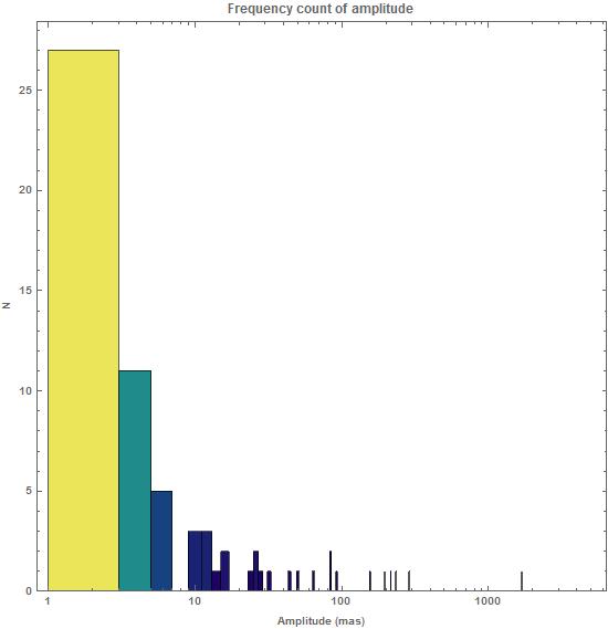
Figure 1: The frequency count for the amplitudes (in milliarcseconds: mas) of 110 significant tide modes of the LARES satellite.

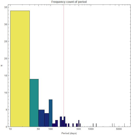
Figure 2: The frequency count for the periods (in days) of 110 tide modes for the LARES satellite.

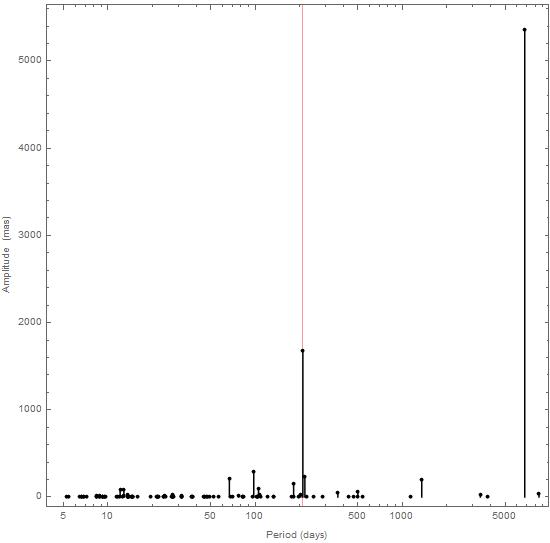
Figure 3: The amplitude vs period for the modes of Figure 1 and 2.

Similar estimations for the tides’ amplitude, period and mutual dependence of the two latter parameters but for LAGEOS and LAGEOS-2, are exhibited in Figures 4-6 and 7-9, respectively. The following input parameters have been used for the orbits of LAGEOS and LAGEOS-2 satellites:

Parameters	LAGEOS	LAGEOS-2
a	12270 km	12163 km
e	0.0045	0.0135
i	$109.84^{o}$	$52.64^{o}$
P	0.1566 days	0.1545 days
${\it P(\Omega)}$	1,043.67 days	-569.21 days
${\it P(\omega)}$	1,707.62 days	821.79 days

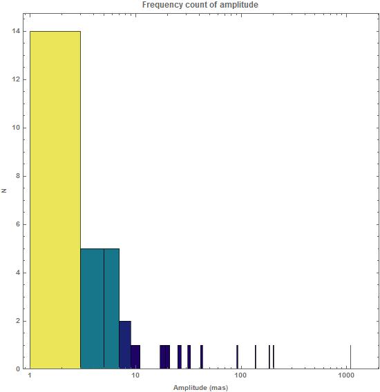
Figure 4: The same as in Figure 1, but for LAGEOS satellite.

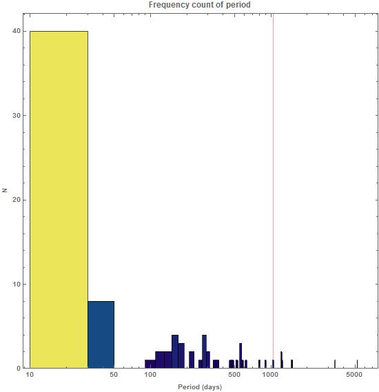
Figure 5: The same as in Figure 2, but for LAGEOS satellite.

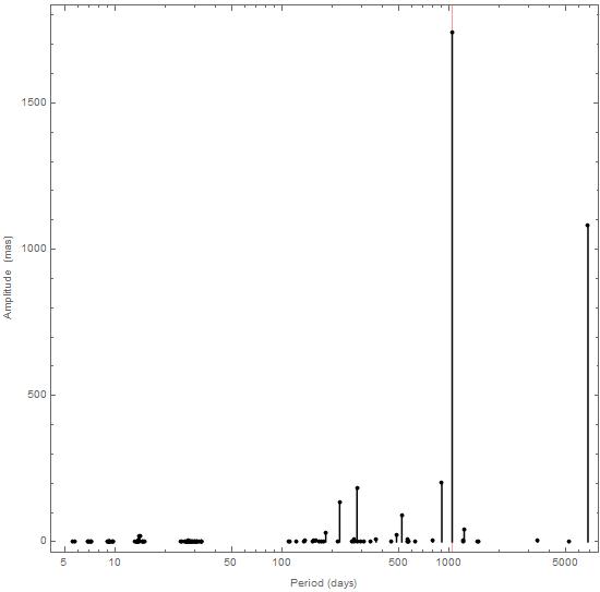
Figure 6: The same as in Figure 3, but for LAGEOS satellite.

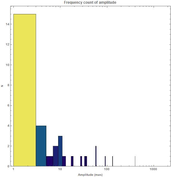
Figure 7: The same as in Figure 1, but for LAGEOS-2 satellite.

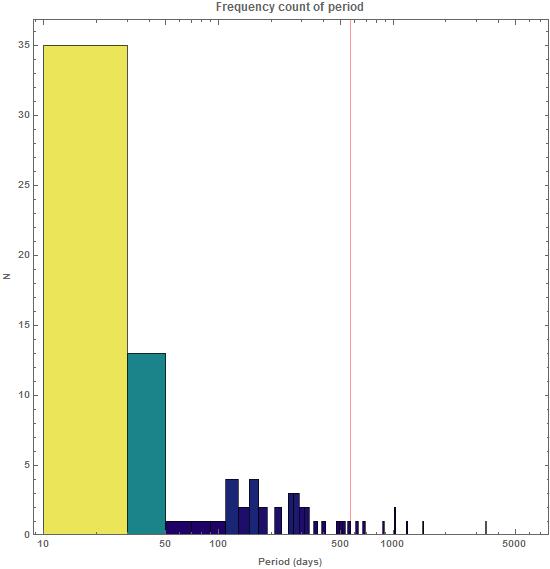
Figure 8: The same as in Figure 2, but for LAGEOS-2 satellite.

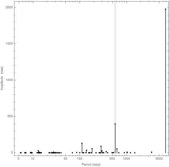
Figure 9: The same as in Figure 3, but for LAGEOS-2 satellite.

1.2 Ocean tides

The gravity of the Moon and Sun generates also ocean tides. The ocean tides can be described by the amplitude $\xi_{a}(\lambda,\phi)$ and phase $\psi(\lambda,\phi)$, both as a function of geocentric longitude and latitude ($\lambda$,$\phi$).

$$\zeta(\lambda,\phi)=\xi_{a}(\lambda,\phi)cos(\theta_{a}+\chi-\psi(\lambda,\phi))$$ (12)

Eq.(12) can be represented via real valued series of prograde and retrograde waves of tides NSWC ; Cart91 ; Ray1999 ; Wu2012

$$\zeta(\phi,\lambda,t)=\sum_{l,m}\{D^{+}_{lm}\cos(\nu t+m\phi-\psi^{+}_{lm})+D^{-}_{lm}\sin(\nu t-m\phi-\psi^{-}_{lm})\}P^{m}_{l}(\cos\lambda)$$ (13)

Those waves can be treated as disturbance to the Earth’s gravitational potential by the term NSWC ; GEMT1 ; EGM96 ; FES2004

$$V_{O}(r,\phi,\lambda)=4{\pi}G\rho_{w}R\sum_{l=0}^{\infty}\sum_{m=-l}^{l}\sum_{-}^{+}{\left(\frac{R}{r}\right)}^{l+1}\frac{(1+\tilde{k_{l}})D_{lm}^{\pm}}{2l+1}P_{lm}(\cos\lambda)\cos(\eta_{lm}^{\pm}(\nu))$$ (14)

where $\rho_{w}=1023\,\,kg/m^{3}$ is the ocean water mean density.

With similar derivations as for the Earth’s tides, one can define the perturbations of the ascending node induced by the ocean tides with amplitudes

$${\Delta\Omega}^{O}_{lmpq}=\frac{720{\rho}_{w}}{\sin(i)}\sqrt{\frac{GR^{2l+4}}{Ma^{2l+3}(1-e^{2})}}\frac{dF_{lmp}(i)}{di}G_{lpq}(e)\frac{D_{lm}^{\pm}(1+\tilde{k}_{l}(\nu))}{(2l+1)\dot{\Gamma}_{j,lmp}}$$ (15)

where $\tilde{k}_{l}(\nu)$ is the load Love number listed in Farrel72 ; NA11 . We list some values of $\tilde{k}_{l}(\nu)$

$\tilde{k}_{l}(\nu)$	$l=1$	$l=2$	$l=3$	$l=4$	$l=5$
	-0.3075	-0.1950	-0.1320	-0.1032	-0.0892

Several models for the ocean tides have been developed i.e. NSWC, EGM96, GOT99, FES2004 (see NSWC ; EGM96 ; Ray1999 ; FES2004 ). Among the two recent models - GOT99 and GOT4.7 - the latter uses more observational data and, particularly, it describes more accurately longer period ocean tides like the mode 056.554. Below we use GOT4.7 to obtain the ocean tides for the the LARES satellite. We are only interested in long periodic modes that do not contain mean anomaly $\mu$, and consider only the modes obeying the condition $l-2p+q=0$.

Table 4. Amplitudes $\Delta\Omega$ and periods of the perturbations for the LARES satellite
by the Moon and Sun induced tides of the ocean.
$l=2$,$p=1$,$q=0$
	Mode	Period(days)	${\Delta\Omega}_{O}(mas)$
$\Omega_{1}$	055.565	6798.3636	315.2685
$S_{a}$	056.554	365.2596	2.9845
$S_{sa}$	057.555	182.6211	9.3936
$M_{m}$	065.455	27.5546	1.4703
$M_{f}$	075.555	13.6608	1.2401
$M_{tm}$	085.455	9.1329	0.1592
$2Q_{1}$	125.755	-6.6434	-0.1130
$\sigma_{1}$	127.555	-6.8649	-0.1389
$Q_{1}$	135.655	-8.7540	-0.9950
$O_{1}$	145.555	-12.8301	-6.6186
$M_{1}$	155.655	-24.3718	-0.8842
$\pi_{1}$	162.556	-77.2026	-0.8812
$P_{1}$	163.555	-97.8938	-18.9394
$S_{1}$	164.555	-133.7391	-1.4276
$K_{1}$	165.555	-211.0000	-121.0278
$\psi_{1}$	166.554	-499.6108	-2.2555
$\phi_{1}$	167.555	1357.8063	10.8730
$J_{1}$	175.455	31.6934	0.8884
${Oo}_{1}$	185.555	14.6065	0.1928
$2N_{2}$	235.755	-6.4406	-0.2312
$\mu_{2}$	237.555	-6.6486	-0.2831
$N_{2}$	245.655	-8.4053	-2.0030
$\nu_{2}$	247.455	-8.7630	-0.3898
$M_{2}$	255.555	-12.0947	-13.2661
$L_{2}$	265.455	-21.5567	-0.5843
$T_{2}$	272.556	-56.5219	-1.3064
$S_{2}$	273.555	-66.8695	-26.1269
$K_{2}$	275.555	-105.5000	-11.1390
$\eta_{2}$	285.455	37.2954	0.1798

For modes with parameters ($l=3,p=1,q=-1$) the Eccentricity Function $G_{lpq}(e)\approx e$ for the eccentricity of LARES’s orbit $e=0.0008$, therefore although $D_{lm}^{\pm}$ harmonic parameters of tides can be as high as for ($l=2,p=1,q=0$), their amplitudes are far smaller.

Table 5. Amplitudes $\Delta\Omega$ and periods of the perturbations for the LARES satellite
by the Moon and Sun induced tides of the ocean.
$l=3$,$p=1$,$q=-1$
	Mode	Period(days)	${\Delta\Omega}_{O}(mas)$
$\Omega_{1}$	055.565	-404.7425	-0.00014
$S_{a}$	056.554	8334.8975	0.00051
$S_{sa}$	057.555	349.8929	0.00013
$M_{m}$	065.455	29.6966	0.00009
$M_{f}$	075.555	14.1674	0.00008
$M_{tm}$	085.455	9.3566	0.00001
$2Q_{1}$	125.755	-6.5299	0.00002
$\sigma_{1}$	127.555	-6.7437	0.00002
$Q_{1}$	135.655	-8.5579	0.00012
$O_{1}$	145.555	-12.4132	0.00071
$M_{1}$	155.655	-22.9101	0.00007
$\pi_{1}$	162.556	-64.2230	0.00005
$P_{1}$	163.555	-77.9244	0.00105
$S_{1}$	164.555	-99.0585	0.00045
$K_{1}$	165.555	-135.9224	0.00538
$\psi_{1}$	166.554	-216.4803	0.00007
$\phi_{1}$	167.555	-531.5420	0.00029
$J_{1}$	175.455	34.5608	-0.00009
${Oo}_{1}$	185.555	15.1872	-0.00003
$2N_{2}$	235.755	-6.3338	-0.00029
$\mu_{2}$	237.555	-6.5349	-0.00035
$N_{2}$	245.655	-8.2243	-0.00197
$\nu_{2}$	247.455	-8.5665	-0.00037
$M_{2}$	255.555	-11.7235	-0.00817
$L_{2}$	265.455	-20.4052	-0.00065
$T_{2}$	272.556	-49.2367	-0.00205
$S_{2}$	273.555	-56.9078	-0.04169
$K_{2}$	275.555	-82.6687	-0.01707
$\eta_{2}$	285.455	41.3306	0.00065

Table 6. Amplitudes $\Delta\Omega$ and periods of the perturbations for the LARES satellite
by the Moon and Sun induced tides of the ocean.
$l=4$,$p=2$,$q=0$
	Mode	Period(days)	${\Delta\Omega}_{O}(mas)$
$\Omega_{1}$	055.565	6798.3636	27.03953
$S_{a}$	056.554	365.2596	0.25527
$S_{sa}$	057.555	182.6211	0.80559
$M_{m}$	065.455	27.5546	0.18429
$M_{f}$	075.555	13.6608	0.21620
$M_{tm}$	085.455	9.1329	0.02776
$2Q_{1}$	125.755	-6.6434	-0.00331
$\sigma_{1}$	127.555	-6.8649	-0.00410
$Q_{1}$	135.655	-8.7540	-0.03139
$O_{1}$	145.555	-12.8301	-0.23620
$M_{1}$	155.655	-24.3718	-0.03316
$\pi_{1}$	162.556	-77.2026	-0.03556
$P_{1}$	163.555	-97.8938	-0.77122
$S_{1}$	164.555	-133.7391	-0.05713
$K_{1}$	165.555	-211.0000	-5.02186
$\psi_{1}$	166.554	-499.6108	-0.09452
$\phi_{1}$	167.555	1357.8063	0.46048
$J_{1}$	175.455	31.6934	0.04318
${Oo}_{1}$	185.555	14.6065	0.01162
$2N_{2}$	235.755	-6.4406	-1.29603
$\mu_{2}$	237.555	-6.6486	-1.57910
$N_{2}$	245.655	-8.4053	-10.78670
$\nu_{2}$	247.455	-8.7630	-2.08704
$M_{2}$	255.555	-12.0947	-68.39948
$L_{2}$	265.455	-21.5567	-2.93874
$T_{2}$	272.556	-56.5219	-6.63498
$S_{2}$	273.555	-66.8695	-133.12218
$K_{2}$	275.555	-105.5000	-58.39958
$\eta_{2}$	285.455	37.2954	1.03664
$M_{4}$	455.555	-6.0473	-0.16397

2 Conclusions

110 significant Earth’s tide modes for the LARES satellite were obtained using the perturbative methods of celestial mechanics and the recent data on the satellite’s orbit. The significant ocean modes were also represented. Note, that for modes of periods exceeding about a year the elasticity effects iers2010 have to be considered in more details. Tidal modes together with non-gravitational effects such as the Yarkovsky-Rubincam effect, are among the main orbital perturbations of laser-ranged satellites; see the randomness analysis of the residuals of the LAGEOS satellites in EPL .

The obtained periods and the amplitudes of the Earth’s modes for LARES were represented in a way, that the mutual relevance of the modes is explicitly revealed. The detailed knowledge of the Earth’s tide modes, i.e., their periods and amplitudes in the nodal longitude of LARES, LAGEOS and LAGEOS 2, is relevant to increase the accuracy in the test of frame-dragging and to estimate the uncertainty of this test and, hence, in probing General Relativity.

We acknowledge the useful comments by the referees. I.C., A.P. and G.S. gratefully acknowledge the Italian Space Agency for the support of the LARES and LARES 2 space missions under agreements No. 2017-23-H.0 and No. 2015-021-R.0. We are also grateful to the International Ranging Service, ESA, AVIO and ELV.

References

- (1) I. Ciufolini and J.A. Wheeler, Gravitation and Inertia, Princeton University Press, 1996
- (2) I. Ciufolini, Nature 449, 41 (2007)
- (3) I. Ciufolini, et al., Eur. Phys. J. Plus 127, 133 (2012)
- (4) I. Ciufolini, V.G. Gurzadyan, R. Penrose, A. Paolozzi, in: Low Dimensional Physics and Gauge Principles, Matinyan Festschrift, p. 93, World Scientific, 2013
- (5) I. Ciufolini, et al., Eur. Phys. J. Plus 130, 133 (2015)
- (6) I. Ciufolini, et al., Eur. Phys. J. C, 76, 120 (2016)
- (7) D. Brouwer, G.M. Clemence, Methods of Celestial Mechanics, Academic Press, New York and London, 1961
- (8) W. M. Kaula, Theory of Satellite Geodesy, Blaisdell Publishing Company, Waltham, 1966
- (9) B. Bertotti, and M. Carpino, in Measurement of the Gravitomagnetic Field Using a Pair of Laser Ranged Satellites, ASI final report, pp. 105, Frascati, 1989
- (10) L. Iorio, Cel. Mech. Dyn. Astron., 79, 201 (2001)
- (11) Petit, G., and Luzum, B., IERS Conventions, IERS Technical Note 36, 79 pp., Frankfurt am Main: Verlag des Bundesamts fuur Kartographie und Geodcurrency sie, 2010
- (12) D. E. Cartwright, R. J. Tayler, Geophys. J. R. Astron. Soc., 23, 45 (1971)
- (13) D. E. Cartwright, A. C. Edden, Geophys. J. R. Astron. Soc., 33, 253 (1973)
- (14) A. E. H. Love, A Treatise on the Mathematical Theory of Elasticity, Dover, New York, 1926
- (15) A. T. Doodson, Proc. Roy. Soc. A., 100, 305 (1921)
- (16) V. G. Gurzadyan, et al, Int. J. Mod. Phys. D, 26, 1741020 (2017)
- (17) V. G. Gurzadyan, et al, EPL, 102 60002 (2013)
- (18) R.D. Ray, B.V. Sanchez, Radial Deformation of the Earth by Oceanic Tidal Loading, NASA Technical Memorandum 100743, Goddard Space Flight Center Greenbelt, Maryland 20771, (1989)
- (19) D. E. Cartwright, R.D. Ray, B.V. Sanchez, Oceanic Tide Maps and Spherical Harmonic Coefficients from Geosat Altimetry, NASA Technical Memorandum 104544, Goddard Space Flight Center Greenbelt, Maryland 20771, (1991)
- (20) R. D. Ray, A Global Ocean Tide Model From TOPEX/POSEIDON Altimetry: GOT99.2, NASA/TM-1999-209478, Goddard Space Flight Center Greenbelt, Maryland 20771, (1999)
- (21) B. Wu, Comparison of different ocean tide models especially with respect to the GRACE satellite mission, Studienarbeit im Studiengang Geodäsie und Geoinformatik an der Universität Stuttgart, Universität Stuttgart Geodätisches Institut, (2012)
- (22) C. Christodoulidis, D. E. Smith, R. G. Williamson, S. M. Klosko, Observed Tidal Earth/Moon/Sun Braking in the System, NASA Technical Memorandum 100677, Goddard Space Flight Center Greenbelt, Maryland 20771, (1987)
- (23) F.G. Lemoine, et al., The Development of the Joint NASA GSFC and the National Imagery and Mapping Agency (NIMA) Geopotential Model EGM96, NASA/1998, 206861, Goddard Space Flight Center Greenbelt, Maryland 20771, (1998)
- (24) W. E. Farrell, Revs. Geophys. Space Phys., 10, 761 (1972)
- (25) S.-H. Na, J. Baek, Computation of the Load Love Number and the Load Green’s Function for an Elastic and Spherically Symmetric Earth, J. Korean Phys. Soc., 58 5 (2011)
- (26) F. Lyard, F. Lefevre, T. Letellier, O. Francis, Ocean Dynamics 56, 394 (2006)