Dominant role of shear-strain-induced admixture in spin-flip processes in self-assembled quantum dots

Abstract

We study theoretically the spin-flip relaxation processes for a single electron in a self-assembled InAs/GaAs quantum dot and show that the dominant channel is the spin admixture induced by symmetry-breaking shear strain. This mechanism, determined within the 8-band envelope-function $\bm{k}\!\cdot\!\bm{p}$ theory, can be mapped onto two effective spin-phonon terms in a conduction-band (effective mass) Hamiltonian that have a similar structure and interfere constructively. Unlike the Dresselhaus coupling, which dominates spin relaxation in larger, unstrained dots, the shear strain contribution cannot be modeled by a generic, standard term in the Hamiltonian but rather relies on the actual strain distribution in the quantum dot.

I Introduction

Dynamics and decoherence of spins in quantum dots (QDs) has been in the focus of both experimental and theoretical studies for several years. This research activity is motivated by the scientific interest in this non-trivial and still not fully understood problem, as well as the promise it holds for possible applications in spintronics and quantum information processing loss98 ; recher00 . The latter is fed by the experimental results showing very long life times of confined spins that raise hopes for their applications as spin memories kroutvar04 and by the development of manufacturing and control technologies that allow one to coherently drive quantum spin states in a desired way koppens06 ; Nowack_Science07 .

Among various QD systems, self-assembled structures show many advantageous features for spin dynamics. In contrast to, e.g., gate-defined lateral or vertical QDs, they are optically active, allowing one to apply optical control approach originally developed for bulk semiconductors kikkawa98 and to use light fields to prepare, detect and control spin states on very short time scales dutt05 ; greilich06c ; Atature2006b ; Kroner2008a ; Xu2008 ; Dubin2008 ; Ramsay2008 ; brunner09 ; Godden2012a (see Refs. [gywat10, ; Ramsay2010, ; Warburton2013, ; DeGreve_RPP13, ; Gao2015, ] for a review). Spin relaxation and dephasing in self-assembled QDs is of particular interest, since these decoherence phenomena set the ultimate limit on the functionality of any nanoscopic spin-based devices. Experiments show exciton spin life times much longer than the recombination times mackowski04 and electron spin relaxation times in the range from nanoseconds Pal2009 to microseconds Heiss2010 or even milliseconds kroutvar04 ; lu10 , depending on the material systems and experimental details. The measured spin coherence times are much shorter, on the order of nanoseconds, which is due to hyperfine-induced dephasing and ensemble inhomogeneity greilich06c ; Akimov2006a ; syperek11 .

Theoretical description of electron spin flip processes in QDs was initially formulated for a lateral gate-defined GaAs structure both for transitions within the ground state Zeeman doubletkhaetskii01 and for relaxation from higher energy levels khaetskii00 . For those structures, the dominant mechanism of spin relaxation was shown to be the admixture mechanism due to the Dresselhaus spin-orbit coupling: an electron state with a certain nominal spin orientation has a contribution of states with inverted spin, which makes it possible for the phonons to couple it to the states with a nominally opposite spin orientation. Due to the time-inversion symmetry, in the resulting effective carrier-phonon Hamiltonian for the Zeeman doublet, the terms that are even in the magnetic field $\bm{B}$ have to vanish, which leads to the characteristic $\sim B^{5}$ dependence of the spin-flip rate. Two other mechanisms invoked in Refs. [khaetskii00, ] and [khaetskii01, ], of much lesser importance for large lateral dots, had a formal structure of a direct spin-phonon coupling and were interpreted as the spin-orbit splitting of the electron spectrum due to the strain field produced by the acoustic phonons and as the strain-induced modification of the electron Landé factor. In later literature, an additional “ripple mechanism” has been invoked, related to the phonon-induced motion of the QD interfacewoods02 ; Alcalde2005 . On the other hand, the generic description of spin-phonon coupling, derived within the formal $\bm{k}\!\cdot\!\bm{p}$ approach from the phonon-related contributions to the fundamental spin-orbit Hamiltonian pavlov65a ; Pavlov1967 , can also be applied to nanostructures in the effective mass and envelope function approximations Alcalde2004 ; Romano2008 ; Wang2012 .

Based on these results, the most common theoretical approach followed in numerous studies, including those devoted to the electron relaxation in self-assembled structures woods02 ; Westfahl2004 ; Cheng2004 ; Alcalde2004 ; Romano2008 ; Zipper2011 ; Wang2012 ; Li2014 , is to derive the electron spin relaxation rates from a simple model of confinement potential within the single-band effective mass approximation and the usual Dresselhaus coupling or other generic spin-orbit coupling terms. In order to improve the accuracy with which the spin-orbit admixtures to the wave functions are treated, it was proposedwei12 to use an atomistic pseudopotential theory for the calculation of wave functions, while the standard carrier-phonon coupling was used for the transitions, thus yielding a more exact theory within the admixture paradigm. The predictions of the admixture model, in particular the $B^{5}$ dependence of the spin relaxation rate, have also been invoked in the interpretation of experimental results that in fact showed such behavior lu10 ; kroutvar04 , apparently confirming the universal character of those theoretical conclusions.

As the relative strengths of various spin relaxation channels strongly depend on the system parameters, in particular on the energetic separation of the excited states, there seems to be no reason for a particular ordering of these channels to hold universally. Moreover, in self-assembled systems, a single-band effective mass approach is just the simplest approximation. Applying a more general multi-band $\bm{k}\!\cdot\!\bm{p}$ theory in the standard envelope-function approachwinkler03 not only offers quantitatively more accurate wave functions but also allows one to systematically include spin-orbit couplings and strain fields. In this way, all the channels of spin relaxation can be included on the same footing. The standard quasi-degenerate perturbation theory (Löwdin elimination of the valence bands) yields an effective electron Hamiltonian. This allows one to relate the electron spin-flip channels proposed in the literature to particular terms in the well-established $\bm{k}\!\cdot\!\bm{p}$ Hamiltonian as well as to verify the predictions based on various mechanisms, estimate the effective constants and assess the relative importance of various couplings for the electron spin-flip process in a self-assembled QD.

In this paper, we present the results of $\bm{k}\!\cdot\!\bm{p}$ modeling of electron spin relaxation in InGaAs/GaAs self-assembled QDs. First, we classify the terms responsible for spin-flip processes at the level of an 8-band theory and show that spin relaxation between the Zeeman sub-levels of the ground state is dominated by the admixture mechanism induced by shear strain and valence-band deformation potentials. By perturbatively reducing the model to an effective description of the conduction band, we show that this mechanism corresponds to a strain-dependent anisotropic contribution to the electron $g$-factor that leads to spin mixing.

The paper is organized as follows. In Sec. II we define the model of the QD system. In the central Sec. III we present, compare and interpret the results for spin relaxation via various channels. Sec. IV concludes the paper.

II Model

We consider a flat-bottom lens-shaped, self-assembled InAs QD placed in a GaAs matrix, assuming a uniform composition of 100% InAs inside the QD and the wetting layer (WL). The base radius of the dot is 12 nm and the height is 4.2 nm, while the height of the WL is 0.6 nm. The system is placed in a magnetic field oriented in the growth direction.

The electron wave functions are obtained by diagonalizing the 8-band $\bm{k}\!\cdot\!\bm{p}$ Hamiltonian in the envelope function approximation winkler03 ; Willatzen2009 . The model includes the kinetic terms up to the second order both within the bands and in the band-off-diagonal blocks coupling the conduction and valence bands. We account for the strain within the continuous elasticity approachpryor98b in the linear order.

In the block notation the Hamiltonian has the form

$$H=\left(\begin{array}[]{ccc}H_{\mathrm{6c6c}}&H_{\mathrm{6c8v}}&H_{\mathrm{6c7v}}\\ H_{\mathrm{8v6c}}&H_{\mathrm{8v8v}}&H_{\mathrm{8v7v}}\\ H_{\mathrm{7v6c}}&H_{\mathrm{7v8v}}&H_{\mathrm{7v7v}}\\ \end{array}\right),$$ (1)

where the blocks refer in the standard way to the lowest conduction band (cb, 6c), the $j=3/2$ valence band (vb, 8v) and the $j=1/2$ (spin-orbit split-off) vb (7v). Here and in the following we use the notation of Ref. [winkler03, ]. The corresponding blocks are explicitly given bywinkler03 ; eissfeller11

$$H_{\mathrm{6c6c}} =E_{\mathrm{c}}+V_{\mathrm{p}}+a_{\mathrm{c}}\operatorname{Tr}\epsilon$$

$$\quad+\frac{\hbar^{2}}{2m_{0}}\left(k_{x}A^{\prime}_{c}k_{x}+\frac{i}{2}k_{[x}g^{\prime}k_{y]}\sigma_{z}+\mathrm{c.p.}\right),$$ (2a)

$$H_{\mathrm{8v8v}} =E_{\mathrm{v}}-\frac{\hbar^{2}}{2m_{0}}\left\{k_{x}\gamma^{\prime}_{1}k_{x}-2\left(J^{2}_{x}-\frac{1}{3}J^{2}\right)k_{x}\gamma^{\prime}_{2}k_{x}\right.$$

$$\quad-\{J_{x},J_{y}\}k_{\{x}\gamma^{\prime}_{3}k_{y\}}+\mathrm{c.p.}\bigg{\}}$$

$$\quad+\frac{1}{2\sqrt{3}}\left[\{J_{x},J^{2}_{y}-J^{2}_{z}\}\{C_{k},k_{x}\}+\mathrm{c.p.}\right]$$

$$\quad+a_{\mathrm{v}}\operatorname{Tr}\epsilon-b_{\mathrm{v}}\left[\left(J^{2}_{x}-\frac{1}{3}J^{2}\right)\epsilon_{xx}+\mathrm{c.p.}\right]$$

$$\quad-\frac{d_{\mathrm{v}}}{\sqrt{3}}\left[\{J_{x},J_{y}\}\epsilon_{xy}+\mathrm{c.p.}\right]$$

$$\quad-i\frac{\hbar^{2}}{m_{0}}\left[k_{[x}\kappa^{\prime}k_{y]}J_{z}+k_{[x}qk_{y]}J^{3}_{z}+\mathrm{c.p.}\right],$$ (2b)

$$H_{\mathrm{7v7v}} =E_{\mathrm{v}}+V_{\mathrm{p}}+a_{\mathrm{v}}\operatorname{Tr}\epsilon$$

$$\quad-\Delta_{0}-\frac{\hbar^{2}}{2m_{0}}(k_{x}\gamma^{\prime}_{1}k_{x}+\mathrm{c.p.})$$

$$\quad-i\frac{\hbar^{2}}{m_{0}}\left[k_{[x}\kappa^{\prime}k_{y]}\sigma_{z}+\mathrm{c.p.}\right]$$

$$\quad-\left(\mu_{B}B_{z}\sigma_{z}+\mathrm{c.p.}\right),$$ (2c)

$$H_{\mathrm{6c8v}} =\sqrt{3}\bm{T}\cdot\widetilde{\bm{k}}P+i\frac{\sqrt{3}}{2}(T_{x}k_{\{y}B_{\mathrm{8v}}^{+}k_{z\}}+\mathrm{c.p.})$$

$$\quad+\frac{\sqrt{3}}{2}\left[(T_{xx}-T_{yy})\left(\frac{2}{3}k_{z}B_{\mathrm{8v}}^{-}k_{z}\right.\right.$$

$$\quad\left.-\frac{1}{3}k_{x}B_{\mathrm{8v}}^{-}k_{x}-\frac{1}{3}k_{y}B_{\mathrm{8v}}^{-}k_{y}\right)$$

$$\quad-T_{zz}(k_{x}B_{\mathrm{8v}}^{-}k_{x}-k_{y}B_{\mathrm{8v}}^{-}k_{y})\bigg{]}$$

$$\quad+i\sqrt{3}C_{2}(T_{x}\epsilon_{yz}+\mathrm{c.p.}),$$ (2d)

$$H_{\mathrm{6c7v}} =-\frac{1}{\sqrt{3}}\bm{\sigma}\cdot\widetilde{\bm{k}}P-\frac{i}{2\sqrt{3}}(\sigma_{x}k_{\{y}B_{\mathrm{7v}}k_{z\}}+\mathrm{c.p.})$$

$$\quad-i\frac{1}{\sqrt{3}}C_{2}(\sigma_{x}\epsilon_{yz}+\mathrm{c.p.}),$$ (2e)

$$H_{\mathrm{8v7v}} =-\frac{\hbar^{2}}{2m_{0}}\left\{-6(T^{\dagger}_{xx}k_{x}\gamma^{\prime}_{2}k_{x}+\mathrm{c.p.})\right.$$

$$\quad-6(T^{\dagger}_{xy}k_{\{x}\gamma^{\prime}_{3}k_{y\}}+\mathrm{c.p.})\big{\}}$$

$$\quad-i\frac{\sqrt{3}}{2}\left(T^{\dagger}_{yz}\{C_{k},k_{x}\}+\mathrm{c.p.}\right)$$

$$\quad-3b_{\mathrm{v}}\left(T^{\dagger}_{xx}\epsilon_{xx}+\mathrm{c.p.}\right)-\sqrt{3}d_{\mathrm{v}}\left(2T^{\dagger}_{xy}\epsilon_{xy}+\mathrm{c.p.}\right)$$

$$\quad-i\frac{3\hbar^{2}}{2m_{0}}\left[k_{[x}\kappa^{\prime}k_{y]}T^{\dagger}_{z}+\mathrm{c.p.}\right]$$

$$\quad-3\left(\mu_{B}B_{z}T^{{\dagger}}_{z}+\mathrm{c.p.}\right).$$ (2f)

Here $\{\mathcal{O}_{1},\mathcal{O}_{2}\}=\mathcal{O}_{1}\mathcal{O}_{2}+\mathcal{O}_{2}\mathcal{O}_{1}$, $k_{\{i}\mathcal{O}k_{j\}}=k_{i}\mathcal{O}k_{j}+k_{j}\mathcal{O}k_{i}$, $k_{[i}\mathcal{O}k_{j]}=k_{i}\mathcal{O}k_{j}-k_{j}\mathcal{O}k_{i}$ for any operators $\mathcal{O}$, $\mathcal{O}_{1}$, $\mathcal{O}_{2}$; c.p. stands for the cyclic permutation of indices; $E_{\mathrm{c}}$ and $E_{\mathrm{v}}$ are the cb and vb edges, respectively ($E_{0}=E_{\mathrm{c}}-E_{\mathrm{v}}$ is the fundamental band gap in a bulk crystal), $\Delta_{0}$ is the spin-orbit parameter; $\bm{k}=-i\nabla+e\bm{A}/\hbar$, where $\bm{A}$ is the vector potential of the magnetic field $\bm{B}$; $\widetilde{\bm{k}}=\bm{k}(\mathbb{I}-2\epsilon)$; $\epsilon$ is the strain tensor; $V_{\mathrm{p}}$ is the piezoelectric potential including piezoelectric polarization up to second-order terms in structural strain bester06 ; Migliorato2014 with the parameters taken from Ref. [caro15, ]; $m_{0}$ is the free electron mass; $\gamma_{i}^{\prime}$ are the Luttinger parameters with removed contributions from the $\Gamma_{6}$ cb,

$$\gamma^{\prime}_{1}=\gamma_{1}-\frac{E_{P}}{3E_{0}+\Delta_{0}},\;\gamma^{\prime}_{2,3}=\gamma_{2,3}-\frac{1}{2}\frac{E_{P}}{3E_{0}+\Delta_{0}};$$

$\mu_{B}$ is the Bohr magneton; $q$ is the anisotropic contribution to the bulk $g$-factor in the Luttinger Hamiltonian; $\sigma_{i}$ are the Pauli matrices; $J_{i}$ are matrices of the $j=3/2$ representation of angular momentum; $T_{i}$ are matrix representations of a vector operator between $j=1/2$ and $j=3/2$ states, i.e., $T_{x/y}=-(T^{(1)}_{+1}\mp T^{(1)}_{-1})/\sqrt{2}$, $T_{z}=T^{(1)}_{0}$, with the matrix elements of the spherical components $T^{(1)}_{q}$ given in terms of the Clebsch-Gordan coefficients $\langle j_{1}j_{2};m_{1}m_{2}|jm\rangle$ by the Wigner-Eckart theorem, $\langle m|T^{(1)}_{q}|m^{\prime}\rangle=-\sqrt{2/3}\langle 3/2,m^{\prime};1,q|1/2,m\rangle$, for $m=\pm 1/2$, $m^{\prime}=-3/2,\ldots,3/2$; and $T_{ij}=T_{i}J_{j}+T_{j}J_{i}$; $A^{\prime}_{c}$, $g^{\prime}$ and $\kappa^{\prime}$ are given bywinkler03

$$A^{\prime}_{c} \equiv\frac{m_{0}}{m^{\prime}}=\frac{m_{0}}{m^{*}}-\frac{2}{3}\frac{E_{P}}{E_{0}}-\frac{1}{3}\frac{E_{P}}{E_{0}+\Delta_{0}},$$

$$g^{\prime} =2,\quad\kappa^{\prime}=-\frac{1}{3}\left(\gamma^{\prime}_{1}-2\gamma^{\prime}_{2}-3\gamma^{\prime}_{3}+2\right).$$

In order to avoid $A^{\prime}_{c}<0$, which would result in a non-elliptical system birner11 , we use $E_{P}=(m_{0}/m^{*}-1)E_{0}(E_{0}+\Delta_{0})/(E_{0}+2\Delta_{0}/3)$, which guarantees $A^{\prime}_{c}=1$. In view of the inconsistency of the reported values of $q$winkler03 ; lawaetz71 , we follow Ref. [eissfeller12, ] and use the perturbative formula $q=(2/9)E_{Q}\Delta^{\prime}_{0}/[E^{\prime}_{0}(E^{\prime}_{0}+\Delta^{\prime}_{0})]$, where $E_{Q}$, $E^{\prime}_{0}$ and $\Delta^{\prime}_{0}$ are the $14$-band $\bm{k}\!\cdot\!\bm{p}$ parameterswinkler03 ; then $P=\hbar(E_{P}/2m_{0})^{1/2}$. In numerical calculations we use the gauge-invariant discretization schemeandlauer08 for the covariant derivative. The material parameters used in our $\bm{k}\!\cdot\!\bm{p}$ calculations are given in Table 1.

	GaAs	InAs	Interpolation for $\mathrm{In_{x}Ga_{1{\mkern 1.0mu{-}\mkern 1.0mu}x}As}$
$E_{\mathrm{v}}$	$0.0$ eV	$0.21$ eV	linear
$E_{\mathrm{0}}$	$1.519$ eV	$0.417$ eV	$0.417x{\mkern 1.0mu{+}\mkern 1.0mu}1.519(1{\mkern 1.0mu{-}\mkern 1.0mu}x){\mkern 1.0mu{-}\mkern 1.0mu}0.477x(1{\mkern 1.0mu{-}\mkern 1.0mu}x)$
$E^{\prime}_{\mathrm{0}}$	$4.488$ eV	$4.390$ eV	linear
$E_{\mathrm{Q}}$	$17.535$ eV	$18.255$ eV	linear
$m^{*}$	$0.0665m_{0}$	$0.0229m_{0}$	$[0.0229x{\mkern 1.0mu{+}\mkern 1.0mu}0.0665(1{\mkern 1.0mu{-}\mkern 1.0mu}x)$
			${\mkern 1.0mu{-}\mkern 1.0mu}0.0091x(1{\mkern 1.0mu{-}\mkern 1.0mu}x)]m_{0}$
$\Delta$	$0.341$ eV	$0.39$ eV	$0.39x{\mkern 1.0mu{+}\mkern 1.0mu}0.341(1{\mkern 1.0mu{-}\mkern 1.0mu}x){\mkern 1.0mu{-}\mkern 1.0mu}0.15x(1{\mkern 1.0mu{-}\mkern 1.0mu}x)$
$\Delta^{\prime}_{0}$	$0.171$ eV	$0.25$ eV	linear
$a_{\mathrm{c}}$	$-7.17$ eV	$-5.08$ eV	${\mkern 1.0mu{-}\mkern 1.0mu}5.08x{\mkern 1.0mu{-}\mkern 1.0mu}7.17(1{\mkern 1.0mu{-}\mkern 1.0mu}x){\mkern 1.0mu{-}\mkern 1.0mu}2.61x(1{\mkern 1.0mu{-}\mkern 1.0mu}x)$
$a_{\mathrm{v}}$	$1.16$ eV	$1.00$ eV	linear
$b_{\mathrm{v}}$	$-2.0$ eV	$-1.8$ eV	linear
$d_{\mathrm{v}}$	$-4.8$ eV	$-3.6$ eV	linear
$\gamma_{\mathrm{1}}$	$6.98$	$20.0$	$1/\left[(1{\mkern 1.0mu{-}\mkern 1.0mu}x)/6.98{\mkern 1.0mu{+}\mkern 1.0mu}x/20.0\right]$
$\gamma_{\mathrm{2}}$	$2.06$	$8.5$	$1/\left[(1{\mkern 1.0mu{-}\mkern 1.0mu}x)/8.5{\mkern 1.0mu{+}\mkern 1.0mu}x/2.06\right]$
$\gamma_{\mathrm{3}}$	$2.93$	$9.2$	$1/\left[(1{\mkern 1.0mu{-}\mkern 1.0mu}x)/9.2{\mkern 1.0mu{+}\mkern 1.0mu}x/2.93\right]$
$C_{2}$	$3.3$ eV

Table 1: Material parameters used in the calculations. After Refs. [Vurgaftman2001, ; winkler03, ], except for $C_{2}$, which is extracted from the measurement data in Ref. [dyakonov86a, ].

Coupling to acoustic phonons is included in the standard way in the long-wavelength limit, by taking into account the phonon-related contribution to the strain tensor in the $\bm{k}\!\cdot\!\bm{p}$ Hamiltonian, expressing it in terms of the phonon-induced displacements and quantizing the latter. In addition, piezoelectric coupling is taken into account by performing the same procedure on the strain terms entering the Hamiltonian via induced piezoelectric fields. The off-diagonal piezoelectric couplings are discussed in the Appendix and are shown to give negligibly small contribution, hence we do not include them in the Hamiltonian. The Zeeman splitting at 10 T is 1.065 meV, which corresponds to the wave numbers of 0.31 and 0.58 nm^-1 for longitudinal and transverse phonons, respectively. This corresponds to 2.8% and 5.2% of the Brillouin zone, respectively, thus justifying the long wave length approximations, as well as the linear dispersion model.

III Results and interpretation

In this section, we present the results for the transition rate between the states forming the Zeeman doublet of the electron ground state, obtained from the 8-band $\bm{k}\!\cdot\!\bm{p}$ calculations. First, in Sec. III.1, we discuss the general division of the spin-flip channels into two classes. Next, in Sec. III.2 we present the numerical results for the spin-flip rates resulting from various channels. The dominant channel is then related to an effective term in a reduced conduction band Hamiltonian in Sec. III.3.

III.1 Admixture and spin-phonon mechanisms

The purpose of our analysis is to assess the quantitative importance of various spin-flip mechanisms and to identify the leading ones. First, however, let us note that the direct carrier-phonon coupling is spin-conserving and the original conduction-band block of the multi-band $\bm{k}\!\cdot\!\bm{p}$ Hamiltonian is spin-diagonal, which precludes any spin-flip transitions unless the coupling to valence bands is taken into account via a perturbation theory (Löwdin partitioninglowdin51 ). The resulting spin-flip mechanisms that may appear as higher-order perturbations in the effective description of conduction-band electrons can be of two kindskhaetskii00 ; khaetskii01 . The first type are admixture mechanisms, where the spin transition is due to admixture of states with opposite spin, which makes it possible for phonons to couple two such statespikus84 ; khaetskii00 ; khaetskii01 . The second class are spin-phonon mechanisms, resulting from symmetry-lowering phonon-related strain fields, which, combined with the spin-orbit coupling in the valence bands, lead to direct “spin-phonon” terms in the effective conduction-band HamiltonianRoth1960 ; pikus84 .

These two kinds of processes appearing in the effective conduction-band description can be mapped back to the 8-band $\bm{k}\!\cdot\!\bm{p}$ model and used to classify the results of the multi-band modeling. For this purpose, let us split the effective conduction-band Hamiltonian into the spin-diagonal zeroth-order part $H_{0}$, the spin-conserving electron-phonon coupling $V_{0}$, and the perturbative correction resulting from decoupling of the valence band. The latter contains strain-dependent terms, kept up to the linear order, and is not diagonal in spin states. The instantaneous strain field, represented by the strain tensor $\epsilon$, is composed of the static strain due to the system inhomogeneity $\epsilon^{(\mathrm{s})}$ and the phonon-induced contribution $\epsilon^{(\mathrm{ph})}$, which leads to decomposition of the perturbative correction into two spin-non-diagonal terms with generic forms, respectively,

$$H_{1}=\sum_{i=0}^{3}\sum_{jk=1}^{3}\alpha_{ijk}\sigma_{i}\epsilon_{jk}^{(\mathrm{s})},\quad V_{1}=\sum_{i=0}^{3}\sum_{jk=1}^{3}\alpha_{ijk}\sigma_{i}\epsilon_{jk}^{(\mathrm{ph})},$$

where $\sigma_{0}$ is the unit matrix and $\sigma_{i}$ for $i=1,2,3$ are the Pauli matrices. By diagonalizing $H=H_{0}+H_{1}$ and computing phonon-induced transition rates resulting from $V=V_{0}+V_{1}$ one obtains in principle all the spin-conserving and spin-flipping transitions in the system. To the leading order, however, the latter can be induced either by a combination of $H_{1}$ and $V_{0}$ (admixture mechanisms) or $H_{0}$ and $V_{1}$ (spin-phonon mechanisms). It is therefore clear that the distinction between these two classes of processes can be traced back to the place where phonons are coupled into the 8-band model: in the conduction-band block of the multi-band $\bm{k}\!\cdot\!\bm{p}$ Hamiltonian (admixture mechanism) or in the other blocks, mapped onto the conduction band upon Löwdin perturbative decoupling (spin-phonon mechanisms).

III.2 Contributions to the spin-flip rate

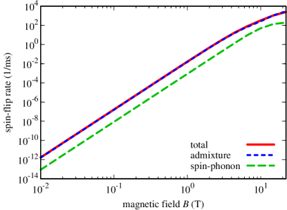
Figure 1: (Color online) The total relaxation rate (solid red line) compared to the rates due to the admixture (dotted blue ) and spin-phonon (dashed green) mechanisms only, as a function of the magnetic field.

In Fig. 1, we show the total spin-flip rate (solid red line), as well as the rates resulting from admixture and spin-phonon mechanisms only (dotted blue and dashed green lines, respectively) as a function of the magnetic field $B$. The admixture mechanisms dominate over the other by over an order of magnitude in the whole range of magnetic fields. Both contributions scale as $B^{5}$ up to about 10 T and at stronger fields the $B$-dependence saturates. The two contributions are almost exactly additive (see Tab. 2 for explicit values).

spin-flip mechanisms and rates (s-1)
total rate   16.31
total admixture	15.42	total spin-phonon	0.874
$d_{\mathrm{v}}$ strain	1.385	$d_{\mathrm{v}}$ phonons	1.169
off-diag strain	3.477	off-diag phonons	0.0237
$d_{\mathrm{v}}$ + off-diag strain	15.36
Dresselhaus	0.238
$C_{2}$ off-diag strain	0.175	$C_{2}$ off-diag phonons	0.0353
“none”	0.185

Table 2: Numerical values of the spin-flip transition rate at $B=1$ T for individual mechanisms and selected combinations of mechanisms.

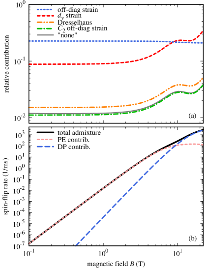
Figure 2: (Color online) (a) Relative contributions to the admixture mechanism from various couplings in the valence band and band-off-diagonal blocks of the $\bm{k}\!\cdot\!\bm{p}$ Hamiltonian as a function of the magnetic field. Each line shows the ratio of the spin flip rate with only one mechanism turned on to the total admixture-induced rate shown in Fig. 1. The thin gray solid line shows the results for all the explicit terms turned off. (b) Contributions of the couplings to different phonon branches as a function of the magnetic field.

The spin-non-conserving admixture can originate either from the Dresselhaus spin-orbit coupling, represented by quadratic terms in $H_{\mathrm{6c8v}}$ and $H_{\mathrm{6c7v}}$ (which is the dominant mechanism in large QDs khaetskii01 ), or from various terms in the valence band, reflecting spin-orbit couplings in a nanostructure, where the crystal symmetry is broken on the mesoscopic level by composition inhomogeneity and strain. In order to determine the dominant contribution in a self-assembled QD, we have studied the spin-flip transition rate for individual contributions to the admixture channel. To this end, we have identified terms in the $\bm{k}\!\cdot\!\bm{p}$ Hamiltonian that lead to spin relaxation via the admixture mechanism (with carrier-phonon coupling via diagonal terms in the conduction band only) and calculated the rate with all these terms switched off in our computational model, except for a single one. The results are shown in Fig. 2(a), where we plot the contributions relative to the total admixture-induced rate. One can see that no single contribution dominates the overall rate. The two most-important ones stem from the shear strain terms that are linear in both momentum and strain in the band-off-diagonal blocks of the $\bm{k}\!\cdot\!\bm{p}$ Hamiltonian $H_{\mathrm{6c8v}}$ and $H_{\mathrm{6c7v}}$ (dashed blue line, labeled “off-diag strain” in Fig. 2(a)) and from the terms in the valence-band blocks $H_{\mathrm{8v8v}}$ and $H_{8v7v}$ proportional to the deformation potential $d_{\mathrm{v}}$ (dashed red line). In order to facilitate quantitative comparison, the rates at $B=1$ T are listed in Tab. 2. The rate obtained when both the dominant channels are turned on is nearly equal to the total rate for admixture mechanisms, while the other mechanisms yield less than 1% of the rate. Note that these two major rates are not additive; in fact, their joint effect is larger than expected even assuming constructive interference of transition amplitudes (which is indeed the case, see Sec. III.3 for more insight). The reason is the large impact of the strain terms in $H_{\mathrm{6c8v}}$ and $H_{\mathrm{6c7v}}$ on the electron $g$-factor: with these terms on, the Zeeman splitting increases by 77% (from 61 to 108 $\mathrm{\SIUnitSymbolMicro}$eV), which enhances relaxation due to growing phonon spectral density at higher frequencies.

The contribution of the remaining channels is very small and leads altogether to a 0.4% correction to the result. This is mostly due to a small Rashba contribution from the overall valence-band-edge inhomogeneity, piezoelectric field in the valence band, and interfaces, which cannot be switched off in our numerical model and remains after all the other explicit couplings are removed; this is represented by the thin solid grey line labeled “none” in Fig. 2(a). Actually, the effect of interfaces is dominant: switching the piezoelectric field in the valence band off reduces this contribution by 3% only. The familiar Dresselhaus coupling ($B_{\mathrm{7v}}$ and $B_{\mathrm{8v}}$ terms in $H_{\mathrm{6c8v}}$ and $H_{\mathrm{6c7v}}$) adds some 50% to this Rashba spin-flip rate. The strain terms proportional to the $C_{2}$ deformation potential contribute negligibly and turn out to interfere destructively with the Rashba part, slightly decreasing the total rate when switched on. These results are in strong contrast to what was found for large QDs in a simple single-band confinement model (corresponding to unstrained, gated QDs) khaetskii01 , where the single Dresselhaus coupling was shown to dominate.

In Fig. 2(b), we have compared the contributions from the deformation-potential(DP, short-dashed orange line) and piezoelectric (PE, dashed blue line) couplings to phonons in $H_{\mathrm{6c6c}}$, which may lead to spin flip in the admixture mechanisms. Up to about 5 T the total rate (black solid lines), as well as its individual components (not shown in the plot) are nearly entirely due to the piezoelectric coupling. As a result, all the rates scale with the magnetic field as $B^{5}$. Deformation-potential coupling produces a $B^{7}$ contribution that is negligible at low and moderate fields but becomes important from about 10 T.

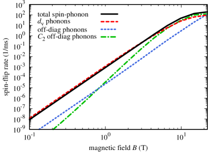
Figure 3: (Color online) Contributions to the spin-phonon mechanism from various phonon couplings in the valence band as a function of the magnetic field.

In Fig. 3 we show selected contributions to the spin-phonon mechanism. Here, the total rate due to this mechanism is clearly dominated by one coupling: the terms proportional to $d_{\mathrm{v}}$ in the valence blocks (with some destructive interference with the other channels). The couplings in off-diagonal blocks have much less importance here at low and moderate fields. However, while the dominant coupling shows a $B^{5}$ behavior up to about 5 T, the $C_{2}$ coupling grows as $B^{7}$ in the range of fields shown (it has a $B^{5}$ to $B^{7}$ crossover at about 0.2 T) and becomes relatively important at field magnitudes of a few Tesla.

III.3 Interpretation in terms of an effective Hamiltonian for the conduction band

We shall now relate the dominant spin-flip contributions to the effective strain-related corrections to the electron Hamiltonian, most of which have been known in different contexts in literature.

Perturbative decoupling of the valence band leads to a correction to the conduction band Hamiltonian, the relevant part of which can be written asMielnik-Pyszczorski2017

$$H_{\mathrm{eff}}=S\mathcal{D}^{-1}S^{{\dagger}},$$ (3)

where $S=\sum_{jl}k_{j}(\delta_{jl}-\epsilon_{jl})\mathcal{T}_{l}P+iC_{2}\sum_{j}\epsilon_{j}\mathcal{T}_{j}$. Here, $\mathcal{T}_{i}=\sqrt{3}T_{i}\oplus(-1/\sqrt{3})\sigma_{i}$ (a $2\times 6$ matrix), $\epsilon_{x}\equiv\epsilon_{yz}$ etc. (by cyclic permutations), $\mathcal{D}=\chi_{\mathrm{c}}\mathbb{I}_{6\times 6}-\widetilde{H}_{\mathrm{v}}$ represents the structure of the valence band, with $\widetilde{H}_{\mathrm{v}}$ approximating the $6\times 6$ valence-band block of the $\bm{k}\!\cdot\!\bm{p}$ Hamiltonian, renormalized by the Löwdin procedure (the details can be found in Ref. [Mielnik-Pyszczorski2017, ], but are not relevant here), and $\chi_{\mathrm{c}}$ is the local conduction band edge (neglecting magnetic contributions, the conduction band block $H_{\mathrm{6c6c}}$ [Eq. 2a] is proportional to unit matrix and can be represented by a scalar function $\chi_{\mathrm{c}}$).

In order to extract the admixture contribution of the terms proportional to $d_{\mathrm{v}}$, we write $\mathcal{D}=\mathcal{D}_{0}-H_{\mathrm{v}}^{(\mathrm{dv})}$, where $\mathcal{D}_{0}=\mathrm{diag}(E_{\mathrm{g}},E_{\mathrm{g}},E_{\mathrm{g}},E_{\mathrm{g}},E_{\mathrm{g}}+\Delta_{\mathrm{SO}},E_{\mathrm{g}}+\Delta_{\mathrm{SO}})$ is a diagonal approximation to $\mathcal{D}$ accounting for the major position-dependent band-edge shifts due to composition and strain (heavy-light hole splitting could be included here as well, in order to slightly improve accuracy, but is neglected for simplicity), and

$$H_{\mathrm{v}}^{(\mathrm{dv})}=-\sqrt{3}d_{\mathrm{v}}\epsilon^{(\mathrm{s})}_{xy}\left(\begin{array}[]{cc}\frac{1}{3}\left\{J_{x},J_{y}\right\}&2T_{xy}^{{\dagger}}\\ 2T_{xy}&0\end{array}\right)+\mathrm{c.p.}$$

is the part of the valence-band block proportional to $d_{\mathrm{v}}$. Here, the blocks of the matrix notation refer to the $\Gamma_{\mathrm{8v}}$ (heavy- and light-hole) and $\Gamma_{\mathrm{7v}}$ (spin-orbit split-off) bands. Substituting this approximate form of $\mathcal{D}$ to Eq. 3, one gets for the relevant part of the conduction band Hamiltonian

$$H_{\mathrm{eff}}^{(\mathrm{dv})}=$$

$$\bm{k}\cdot\bm{\sigma}\frac{2\sqrt{3}P^{2}d_{\mathrm{v}}}{E_{\mathrm{g}}(E_{\mathrm{g}}+\Delta_{\mathrm{SO}})}\left(T_{xy}\epsilon^{(\mathrm{s})}_{xy}+\mathrm{c.p.}\right)\bm{T}^{{\dagger}}\!\cdot\bm{k}+\mathrm{H.c.}$$

$$-\bm{k}\cdot\bm{T}\frac{\sqrt{3}P^{2}d_{\mathrm{v}}}{E_{\mathrm{g}}^{2}}\left(\left\{J_{x},J_{y}\right\}\epsilon^{(\mathrm{s})}_{xy}+\mathrm{c.p.}\right)\bm{T}^{{\dagger}}\!\cdot\bm{k},$$

where we omitted the strain-related contributions to $S$, in order to keep the result linear in strain. The spin-dependent contributions result from the antisymmetric parts of the two terms in Eq. III.3, defined as $[T_{j}\mathcal{O}T_{l}]_{\mathrm{as}}\equiv(1/2)(T_{j}\mathcal{O}T_{l}-T_{l}\mathcal{O}T_{j})$ and $[\sigma_{j}\mathcal{O}T_{l}]_{\mathrm{as}}\equiv(1/2)(\sigma_{j}\mathcal{O}T_{l}-\sigma_{l}\mathcal{O}T_{j})$ for any operator $\mathcal{O}$. Substituting the explicit forms of the matrices one finds

$$\left[T_{x}\left\{J_{x},J_{y}\right\}T_{z}\right]_{\mathrm{as}} =4\left[\sigma_{x}T_{xy}T_{z}\right]_{\mathrm{as}}=\frac{i}{3}\sigma_{x},$$

$$\left[T_{z}\left\{J_{x},J_{y}\right\}T_{y}\right]_{\mathrm{as}} =4\left[\sigma_{z}T_{xy}T_{y}\right]_{\mathrm{as}}=\frac{i}{3}\sigma_{y},$$

with other non-zero terms obtained by asymmetry and by cyclic permutation of indices. Neglecting the non-commutativity of $k_{j}$ with $P$, $d_{\mathrm{v}}$, and $E_{\mathrm{g}}$ and using the relations $[k_{j},k_{l}]=-i(e/\hbar)\sum_{n}\varepsilon_{jln}B_{n}$, $eP^{2}/\hbar=\mu_{\mathrm{B}}E_{\mathrm{P}}$, one obtains

$$H_{\mathrm{eff}}^{(\mathrm{dv})}=\frac{1}{2}\mu_{\mathrm{B}}\bm{B}\delta\hat{g}^{(\mathrm{dv})}\bm{\sigma},$$ (5)

where $\delta\hat{g}$ is a tensor with elements

$$\delta g_{jl}^{(\mathrm{dv})}=\frac{2}{\sqrt{3}}\frac{E_{P}d_{\mathrm{v}}\Delta_{\mathrm{SO}}}{E_{\mathrm{g}}^{2}(E_{\mathrm{g}}+\Delta_{\mathrm{SO}})}\epsilon^{(\mathrm{s})}_{jl}$$

and $E_{P}=2mP^{2}/\hbar^{2}$. This strain-induced mixing term is known in literature VanVleck1940 ; Roth1960 and can be interpreted as a correction $\delta g_{jl}^{(\mathrm{dv})}$ to the electron Landé tensor khaetskii00 ; khaetskii01 .

The second largest contribution, which is due to strain terms in the off-diagonal block of the $\bm{k}\!\cdot\!\bm{p}$ Hamiltonian, enters the effective conduction-band Hamiltonian via strain terms proportional to $P$ in $S$. We now approximate $\mathcal{D}\approx\mathcal{D}_{0}$, which yields, up to linear order in strain,

$$H_{\mathrm{eff}}^{(\mathrm{od})}=-\sum_{jnl}k_{j}P\epsilon^{(\mathrm{s})}_{jn}\mathcal{T}_{n}\mathcal{D}_{0}^{-1}\mathcal{T}_{l}Pk_{l}+\mathrm{H.c.}$$ (6)

Again, only the antisymmetric part yields a spin-dependent term. Using the explicit form of $\mathcal{T}_{j}$, one finds

$$\left[\mathcal{T}_{n}\mathcal{D}_{0}^{-1}\mathcal{T}_{l}\right]_{\mathrm{as}}=-\frac{i}{3}\frac{\Delta_{\mathrm{SO}}}{E_{\mathrm{g}}(E_{\mathrm{g}}+\Delta_{\mathrm{SO}})}\sum_{m}\varepsilon_{nlm}\sigma_{m},$$ (7)

from which one gets

$$H_{\mathrm{eff}}^{(\mathrm{od})}=\frac{1}{2}\mu_{\mathrm{B}}\bm{B}\delta\hat{g}^{(\mathrm{od})}\bm{\sigma},$$

where

$$\delta g_{jl}^{(\mathrm{od})}=-\frac{2}{3}\frac{E_{P}\Delta_{\mathrm{SO}}}{E_{\mathrm{g}}(E_{\mathrm{g}}+\Delta_{\mathrm{SO}})}\epsilon^{(\mathrm{s})}_{jl}.$$

This term has exactly the same structure as the previous one, which explains why the two contributions to spin admixture interfere constructively (note that $d_{\mathrm{v}}$ is negative).

The most important mechanism in the class of direct spin-phonon couplings at low and moderate fields, stemming from the $d_{\mathrm{v}}$ terms, can be mapped onto an effective conduction band Hamiltonian exactly in the same way as the $d_{\mathrm{v}}$ term discussed above. The static strain is replaced by $\epsilon^{(\mathrm{ph})}$, expressed in terms of lattice displacements, and expanded in plane-wave modes. Upon quantization of the latter, one obtains an effective spin-phonon coupling Hamiltonian, discussed already in Refs. [khaetskii00, ] and [khaetskii01, ], which describes spin transitions due to phonon-induced dynamical anisotropic modulation of the $g$-factor.

The spin-phonon contribution proportional to $C_{2}$ appears via terms linear in both $C_{2}$ and strain in Eq. 3,

$$H_{\mathrm{eff}}^{(C2)}=iC_{2}\sum_{jl}\epsilon_{j}\mathcal{T}_{j}\mathcal{D}_{0}^{-1}\mathcal{T}_{l}Pk_{l}+\mathrm{H.c.}$$

Using Eq. 7, one immediately finds

$$H_{\mathrm{eff}}^{(C2)}=\frac{1}{3}\sum_{jlm}\varepsilon_{jlm}\left\{\frac{C_{2}\Delta_{\mathrm{SO}}P}{E_{\mathrm{g}}(E_{\mathrm{g}}+\Delta_{\mathrm{SO}})}\epsilon_{j},k_{l}\right\}\sigma_{m}.$$ (8)

A similar term was derived in the context of the calculation of energy spectrum of strained semiconductors bir61 ; pikus84 ; dyakonov86a . It was discussed as a spin-phonon coupling in the analysis of spin relaxation channels in large QDs khaetskii00 ; khaetskii01 , where it was shown to be much less effective than the “$d_{\mathrm{v}}$” spin-phonon channel discussed above. Interestingly, in a simple model of the “particle-in-a-box” confinement with real ground state wave functions, the effective Hamiltonian $H_{\mathrm{eff}}^{(C2)}$ leads to $B^{5}$ dependence of the spin-flip ratekhaetskii01 , while the numerical values from the 8-band $\bm{k}\!\cdot\!\bm{p}$ theory yield a crossover to $B^{7}$ dependence already below 1 T, as discussed in Sec. III.2.

Another spin-phonon term in the effective Hamiltonian appears from off-diagonal piezoelectric couplings to phonons (see Appendix). This term is non-zero only in an inhomogeneous system but even here its effect is small.

IV Conclusions

In this paper we have presented the results of theoretical modeling of spin-flip relaxation between Zeeman sub-levels of a single electron in a self-assembled InAs/GaAs QD. By analyzing the spin relaxation process with 8-band envelope-function $\bm{k}\!\cdot\!\bm{p}$ theory, we have identified individual spin-flip channels divided into two classes: admixture and spin-phonon mechanisms. We have shown that the former dominates, like in large unstrained dots, although not so overwhelmingly (95% of the total rate). However, in sharp contrast to the latter, the dominant channel of spin relaxation in strained self-assembled QDs is spin admixture induced by symmetry-breaking shear strain, which accounts for 99.6% of the total admixture-induced rate. The dominant processes can be mapped onto two different effective spin-phonon terms in a conduction band (effective mass) Hamiltonian that interfere and interplay in a non-trivial way in producing the total spin-flip rate.

The most important practical consequence of our findings is that the dominant contribution to spin relaxation in self-assembled QDs relies on the particular distribution of shear strain in the structure and, therefore, cannot be modeled by a unique standard term in the Hamiltonian. This is in sharp contrast to larger, unstrained dots, where spin relaxation is dominated by the Dresselhaus coupling easily accounted for by the well-known generic spin-orbit term in the Hamiltonian.

The second observation that we find important is that in magnetic fields up to about 5 T the rates of all the important spin-flip channels, both admixture and spin-phonon, are proportional to $B^{5}$. Therefore, this simple characteristics cannot be used as a key to distinguishing the dominant spin-flip mechanisms in an experiment.

Finally, identifying the dominant spin-flip mechanism as being due to strain suggests that considerable enhancement of spin life time may be possible in structures with reduced strain. This is consistent with the results concerning an impurity-bound electron Linpeng2016 , which is a strain-free system, where the dominating spin-flip channels are related to direct spin-phonon and Dresselhaus SO couplings.

Appendix A Off-diagonal piezoelectric couplings

In this Appendix, we derive the general structure of the off-diagonal piezoelectric carrier-phonon couplings and estimate the resulting spin-phonon terms in the effective Hamiltonian for conduction band electrons.

The strain due to phonons, written in the coordinate representation with respect to the electron and in the second quantization with respect to phonons, has the form

$$\epsilon_{ij}\!\left(\bm{r}\right)=\sum_{\bm{q},\lambda}\epsilon_{ij}^{(\bm{q},\lambda)}e^{i\bm{q}\cdot\bm{r}},$$

where

$$\epsilon_{ij}^{(\bm{q},\lambda)}=-\frac{1}{2}\sqrt{\frac{\hbar}{2\rho V\omega_{q,\lambda}}}\\ \times\!\left[\,\!\left(\hat{\bm{e}}_{\bm{q},\lambda}\right){\!}_{i}\,q_{j}+\!\left(\hat{\bm{e}}_{\bm{q},\lambda}\right){\!}_{j}\,q_{i}\right]\!\left(b_{\bm{q},\lambda}+b_{-\bm{q},\lambda}^{{\dagger}}\right).$$ (9)

Here $V$ is the normalization volume of the phonon system, $\hat{\bm{e}}_{\bm{q},\lambda}=-\hat{\bm{e}}_{-\bm{q},\lambda}^{*}$ is the mode polarization, and $b_{\bm{q},\lambda}^{{\dagger}},b_{\bm{q},\lambda}$ are phonon creation and annihilation operators. The resulting piezoelectric potential in a zincblende crystal is then

$$V(\bm{r})=i\sum_{\bm{q}}v^{(\bm{q})}e^{i\bm{q}\cdot\bm{r}},$$

where

$$v^{(\bm{q})}=2\mathcal{E}_{\mathrm{p}}\frac{1}{q^{2}}\sum_{\lambda}\left(q_{x}\epsilon_{yz}^{(\bm{q},\lambda)}+\mathrm{c.p.}\right).$$

The above equation is correct for an inhomogeneous system in the long wave length limit, when the small-scale details become irrelevant and the system can be approximated by a virtual uniform medium characterized by a constant $\mathcal{E}_{\mathrm{p}}=ee_{14}/\epsilon_{0}\epsilon_{s}$, which should be close to the GaAs matrix value of 1.4 eV/nm.

In the envelope-function approach, one separates the mesoscopic length scales (coarse-grained position $\bm{R}$) from the atomic scales (position $\bm{\xi}$ within a unit cell). It is assumed that material parameters vary only on the mesoscopic scales. The matrix elements of a multi-band $\bm{k}\!\cdot\!\bm{p}$ Hamiltonian at a position $\bm{R}$ are then obtained as matrix elements of the original Hamiltonian between the Bloch functions $u_{\mu},u_{\nu}$ corresponding to the two bands $\mu,\nu$, calculated over one unit cell (u.c.) of volume $v$, located at $\bm{R}$. Writing $\bm{r}=\bm{R}+\bm{\xi}$, one obtains the contribution of the piezoelectric coupling to the matrix elements of the $\bm{k}\!\cdot\!\bm{p}$ Hamiltonian

$$V_{\mu\nu}=i\sum_{\bm{q}}v^{(\bm{q})}e^{i\bm{q}\cdot\bm{R}}\left\langle\mu\left|e^{-\bm{q}\cdot\bm{\xi}}\right|\nu\right\rangle_{\mathrm{u.c.}},$$

where

$$\left\langle\mu\left|\mathcal{O}(\bm{\xi})\right|\nu\right\rangle_{\mathrm{u.c.}}=\frac{1}{v}\int_{\mathrm{u.c.}}\mathrm{d}^{3}\bm{\xi}\,u_{\mu}^{*}(\bm{\xi})\mathcal{O}(\bm{\xi})u_{\nu}(\bm{\xi}).$$

In a mesoscopic structure, the magnitude of $\bm{q}$ for phonons that are efficiently coupled to confined carriers is effectively limited to the range $q\lesssim 1/l\ll 1/a$, where $l$ is the spatial extension of the envelope function and $a$ is the lattice constant. Therefore, $\bm{q}\cdot\bm{\xi}\ll 1$ and the exponent can be expanded in series,

$$e^{i\bm{q}\cdot\bm{\xi}}\simeq 1+i\bm{q}\cdot\bm{\xi}-\frac{\!\left(\bm{q}\cdot\bm{\xi}\right)^{2}}{2}.$$

The zeroth-order term is diagonal due to the orthogonality of Bloch functions and for each of the bands reproduces the standard piezoelectric carrier-phonon coupling. The higher-order terms contribute to inter-band couplings, for which the zeroth-order term vanishes.

With the known composition of Bloch functions in terms of atomic orbitals one can relate the required matrix elements to those between angular momentum eigenstates. Here, we will take the standard assumption that the cb states are $s$-type and the vb states are purely $p$-type. Then, due to parity, the linear term in the expansion contributes only to the off-diagonal cb-vb block of the $\bm{k}\!\cdot\!\bm{p}$ Hamiltonian. Denoting $\langle 1/2,1/2,\mathrm{cb}|\xi_{x}|3/2,3/2,\mathrm{vb}\rangle=d_{1}/\sqrt{2}$ one finds from the Wigner-Eckart theorem

$$\left\{\left\langle\mu\left|\bm{\xi}\right|\nu\right\rangle_{\mathrm{u.c.}}\right\}_{\mu,\nu}=\sqrt{3}d_{1}\bm{\mathcal{T}},$$

where $\mu$ and $\nu$ run through the two conduction and six valence bands, respectively. Hence, the resulting first-order Hamiltonian term is

$$H^{(\mathrm{PE,1})} =\sqrt{3}d_{1}\bm{\mathcal{E}}\cdot\bm{\mathcal{T}}+\mathrm{H.c.},$$ (10)

where

$$\bm{\mathcal{E}}(\bm{R})=-\nabla V(\bm{R})=\sum_{\bm{q}}v^{(\bm{q})}\bm{q}e^{i\bm{q}\cdot\bm{R}}$$

is the piezoelectric field.

The quadratic term has non-vanishing matrix elements only between valence band states. Denoting $\langle 3/2,3/2,\mathrm{vb}|\xi_{x}\xi_{y}|3/2,-1/2,\mathrm{vb}\rangle=-id_{2}/\sqrt{3}$, with $d_{2}$ real, one finds the relevant part of the valence-band piezoelectric perturbation

$$H^{(\mathrm{PE,2})}=\frac{i}{6}d_{2}\frac{\partial\mathcal{E}_{y}(\bm{R})}{\partial x}\left(\begin{array}[]{cc}\left\{J_{x},J_{y}\right\}&6T_{xy}^{{\dagger}}\\ 6T_{xy}&0\end{array}\right)+\mathrm{c.p.},$$ (11)

where we neglected terms proportional to $q_{i}^{2}$ that do not induce spin relaxation.

In order to assess the effect of the linear term 10 on the electron spin-flip processes, we go back to Eq. 3, where we extend $S\to S^{\prime}=S+S_{\mathrm{pe}}$ with $S_{\mathrm{pe}}=H^{(\mathrm{PE,1})}$. From the resulting terms we again select the spin-dependent antisymmetric part, according to Eq. 7. The resulting effective Hamiltonian for the conduction band can be written in two equivalent forms

$$H_{\mathrm{eff}}^{\mathrm{(PE,1)}} =-\frac{i}{\sqrt{3}}\frac{\Delta_{\mathrm{SO}}Pd_{1}}{E_{\mathrm{g}}(E_{\mathrm{g}}+\Delta_{\mathrm{SO}})}\bm{\sigma}\cdot\left(\bm{\mathcal{E}\times\bm{k}}\right)+\mathrm{H.c.}$$

$$=\frac{1}{\sqrt{3}}\left[\bm{\mathcal{E}}\times\nabla\frac{\Delta_{\mathrm{SO}}Pd_{1}}{E_{\mathrm{g}}(E_{\mathrm{g}}+\Delta_{\mathrm{SO}})}\right]\cdot\bm{\sigma},$$ (12)

where we used the fact that $\bm{\mathcal{E}}$ is longitudinal. The first equation represents the effective Hamiltonian in the usual Dresselhaus form with the piezoelectric field as the symmetry-breaking factor. The final equation shows explicitly that the block-off-diagonal terms contribute to electron spin-phonon coupling only in an inhomogeneous system. By comparing Eq. A with Eq. 8 one can see that the overall magnitude of the piezoelectric spin-flip term is reduced by a factor $d_{1}\mathcal{E}_{\mathrm{p}}/C_{2}$. In GaAs $d_{1}=0.11$ nm (estimated in a model of hydrogen-like orbitals with equal distribution of wave functions between the anion and the cationChekhovich2011 ; Clementi1963 ). Hence, $d_{1}\mathcal{E}_{\mathrm{p}}/C_{2}=0.047$ and we expect the resulting rate (proportional to the square of the coupling) to be at least three orders of magnitude lower than that resulting from the $C_{2}$ coupling, which is small itself.

The effective Hamiltonian corresponding to Eq. 11 is constructed by closely following the derivation of Eq. 5. One obtains the analogous term

$$H_{\mathrm{eff}}^{(\mathrm{PE,2})}=\frac{1}{2}\mu_{\mathrm{B}}\bm{B}\delta\hat{g}^{(\mathrm{PE,2})}\bm{\sigma},$$

with

$$\delta g_{jl}^{(\mathrm{PE,2})}=-\frac{2}{3}\frac{E_{P}d_{2}\Delta_{\mathrm{SO}}}{E_{\mathrm{g}}^{2}(E_{\mathrm{g}}+\Delta_{\mathrm{SO}})}\frac{\partial\mathcal{E}_{j}}{\partial x_{l}},\quad j\neq l.$$

Comparison to Eq. 5 shows that the piezoelectric term is smaller by a factor $\mathcal{E}_{\mathrm{p}}d_{2}q_{0}/d_{\mathrm{v}}=1.1\times 10^{-4}$, where we used the estimate $d_{2}=9.3\times 10^{-3}$ nm² (obtained in the same way as $d_{1}$ above) and $q_{0}=g\mu_{\mathrm{B}}B/(\hbar c)\approx 0.04$ nm^-1 is the resonant wave vector for a transition between Zeeman sub-levels. It follows that this term is negligible.

References

- (1) D. Loss and D. P. DiVincenzo, Phys. Rev. A 57, 120 (1998).
- (2) P. Recher, E. V. Sukhorukov, and D. Loss, Phys. Rev. Lett. 85, 1962 (2000).
- (3) M. Kroutvar, Y. Ducommun, D. Heiss, M. Bichler, D. Schuh, G. Abstreiter, and J. J. Finley, Nature 432, 81 (2004).
- (4) F. H. L. Koppens, C. Buizert, K. J. Tielrooij, I. T. Vink, K. C. Nowack, T. Meunier, L. P. Kouwenhoven, and L. M. K. Vandersypen, Nature 442, 766 (2006).
- (5) K. C. Nowack, F. H. L. Koppens, Y. V. Nazarov, and L. M. K. Vandersypen, Science 318, 1430 (2007).
- (6) J. M. Kikkawa and D. D. Awschalom, Phys. Rev. Lett. 80, 4313 (1998).
- (7) M. V. Gurudev Dutt, J. Cheng, B. Li, X. Xu, X. Li, P. R. Berman, D. G. Steel, A. S. Bracker, D. Gammon, S. E. Economou, R.-B. Liu, and L. J. Sham, Phys. Rev. Lett. 94, 227403 (2005).
- (8) A. Greilich, R. Oulton, E. Zhukov, I. Yugova, D. Yakovlev, M. Bayer, A. Shabaev, A. Efros, I. Merkulov, V. Stavarache, D. Reuter, and A. Wieck, Phys. Rev. Lett. 96, 227401 (2006).
- (9) M. Atatüre, J. Dreiser, A. Badolato, A. Högele, K. Karrai, and A. Imamoglu, Science 312, 551 (2006).
- (10) M. Kroner, K. M. Weiss, B. Biedermann, S. Seidl, S. Manus, A. W. Holleitner, A. Badolato, P. M. Petroff, B. D. Gerardot, R. J. Warburton, and K. Karrai, Phys. Rev. Lett. 100, 156803 (2008).
- (11) X. Xu, B. Sun, P. R. Berman, D. G. Steel, A. S. Bracker, D. Gammon, and L. J. Sham, Nat. Phys. 4, 692 (2008).
- (12) F. Dubin, M. Combescot, G. K. Brennen, and R. Melet, Phys. Rev. Lett. 101, 217403 (2008).
- (13) A. J. Ramsay, S. J. Boyle, R. S. Kolodka, J. B. B. Oliveira, J. Skiba-Szymanska, H. Y. Liu, M. Hopkinson, A. M. Fox, and M. S. Skolnick, Phys. Rev. Lett. 100, 197401 (2008).
- (14) D. Brunner, B. D. Gerardot, P. A. Dalgarno, G. Wuest, K. Karrai, N. G. Stoltz, P. M. Petroff, and R. J. Warburton, Science 325, 70 (2009).
- (15) T. M. Godden, J. H. Quilter, A. J. Ramsay, Y. Wu, P. Brereton, S. J. Boyle, I. J. Luxmoore, J. Puebla-Nunez, A. M. Fox, M. S. Skolnick, Phys. Rev. Lett. 108, 017402 (2012).
- (16) O. Gywat, H. J. Krenner, and J. Berezovsky, Spins in Optically Active Quantum Dots: Concepts and Methods (Wiley-VCH, Weinheim, 2010).
- (17) A. J. Ramsay, Semicond. Sci. Technol. 25, 103001 (2010).
- (18) R. J. Warburton, Nat. Mater. 12, 483 (2013).
- (19) K. De Greve, D. Press, P. L. McMahon, and Y. Yamamoto, Rep. Prog. Phys. 76, 92501 (2013).
- (20) W. B. Gao, A. Imamoglu, H. Bernien, and R. Hanson, Nat. Photonics 9, 363 (2015).
- (21) S. Mackowski, T. A. Nguyen, T. Gurung, K. Hewaparakrama, H. E. Jackson, L. M. Smith, J. Wrobel, K. Fronc, J. Kossut, and G. Karczewski, Phys. Rev. B 70, 245312 (2004).
- (22) B. Pal and Y. Masumoto, Phys. Rev. B 80, 125334 (2009).
- (23) D. Heiss, V. Jovanov, F. Klotz, D. Rudolph, M. Bichler, G. Abstreiter, M. S. Brandt, and J. J. Finley, Phys. Rev. B 82, 245316 (2010).
- (24) C.-Y. Lu, Y. Zhao, A. N. Vamivakas, C. Matthiesen, S. Fält, A. Badolato, and M. Atatüre, Phys. Rev. B 81, 035332 (2010).
- (25) I. A. Akimov, D. H. Feng, and F. Henneberger, Phys. Rev. Lett. 97, 056602 (2006).
- (26) M. Syperek, D. R. Yakovlev, I. A. Yugova, J. Misiewicz, I. V. Sedova, S. V. Sorokin, A. A. Toropov, S. V. Ivanov, and M. Bayer, Phys. Rev. B 84, 085304 (2011).
- (27) A. V. Khaetskii and Y. V. Nazarov, Phys. Rev. B 64, 125316 (2001).
- (28) A. V. Khaetskii and Y. V. Nazarov, Phys. Rev. B 61, 12639 (2000).
- (29) L. M. Woods, T. L. Reinecke, and Y. Lyanda-Geller, Phys. Rev. B 66, 161318 (2002).
- (30) A. Alcalde, O. Diniz Neto, and G. Marques, Microelectronics J. 36, 1034 (2005).
- (31) S. T. Pavlov and Y. A. Firsov, Fiz. Tv. Tela 7, 2634 (1965) [Sov. Phys. Soild State 7, 2131 (1966)].
- (32) S. T. Pavlov and Y. A. Firsov, Fiz. Tv. Tela 9, 1780 (1967) [Sov. Phys. Solid State 9, 1394 (1966)].
- (33) A. Alcalde, Q. Fanyao, and G. Marques, Physica E 20, 228 (2004).
- (34) C. L. Romano, G. E. Marques, L. Sanz, and A. M. Alcalde, Phys. Rev. B 77, 033301 (2008).
- (35) Z.-W. Wang and S.-S. Li, Solid State Commun. 152, 1098 (2012).
- (36) H. Westfahl, A. O. Caldeira, G. Medeiros-Ribeiro, and M. Cerro, Phys. Rev. B 70, 195320 (2004).
- (37) J. L. Cheng, M. W. Wu, and C. Lü, Phys. Rev. B 69, 115318 (2004).
- (38) E. Zipper, M. Kurpas, J. Sadowski, and M. M. Maśka, J. Phys. Condens. Matter 23, 115302 (2011).
- (39) W.-P. Li, S.-J. Li, J.-W. Yin, Y.-F. Yu, and Z.-W. Wang, Solid State Commun. 192, 1 (2014).
- (40) H. Wei, M. Gong, G.-C. Guo, and L. He, Phys. Rev. B 85, 045317 (2012).
- (41) R. Winkler, Spin-Orbit Coupling Effects in Two-Dimensional Electron and Hole Systems, Vol. 191 of Springer Tracts in Modern Physics (Springer, Berlin, 2003).
- (42) L. C. Lew Yan Voon and M. Willatzen, The k p Method (Springer, Berlin, Heidelberg, 2009).
- (43) C. Pryor, J. Kim, L. W. Wang, A. J. Williamson, and A. Zunger, J. Appl. Phys. 83, 2548 (1998).
- (44) T. Eissfeller and P. Vogl, Phys. Rev. B 84, 195122 (2011).
- (45) G. Bester, A. Zunger, X. Wu, and D. Vanderbilt, Phys. Rev. B 74, 081305 (2006).
- (46) M. A. Migliorato, J. Pal, R. Garg, G. Tse, H. Y. Al-Zahrani, U. Monteverde, S. Tomić, C.-K. Li, Y.-R. Wu, B. G. Crutchley, I. P. Marko, and S. J. Sweeney, AIP Conf. Proc. 1590, 32 (2014).
- (47) M. A. Caro, S. Schulz, and E. P. O’Reilly, Phys. Rev. B 91, 075203 (2015).
- (48) T. Andlauer, R. Morschl, and P. Vogl, Phys. Rev. B 78, 075317 (2008).
- (49) S. Birner, Ph.D. thesis, Technische Universität München, 2011.
- (50) P. Lawaetz, Phys. Rev. B 4, 3460 (1971).
- (51) T. Eissfeller, Ph.D. thesis, Technische Universität München, 2012.
- (52) I. Vurgaftman, J. R. Meyer, and L. R. Ram-Mohan, J. Appl. Phys. 89, 5815 (2001).
- (53) M. I. D’yakonov, V. A. Marushchak, V. I. Perel’, and A. N. Titkov, Zh. Exp. Teor. Fiz. 90, 1123 (1986) [Sov. Phys. JETP 63, 655 (1986)].
- (54) P.-O. Löwdin, J. Chem. Phys. 19, 1396 (1951).
- (55) G. E. Pikus and A. N. Titkov, in Opt. Orientat., edited by F. Meier and B. P. Zakharchenya (Elsevier, Amsterdam, 1984), p. 73.
- (56) L. M. Roth, Phys. Rev. 118, 1534 (1960).
- (57) A. Mielnik-Pyszczorski, K. Gawarecki, and P. Machnikowski, Sci. Rep. 8, 2873 (2018).
- (58) J. H. Van Vleck, Phys. Rev. 57, 426 (1940).
- (59) G. L. Bir and G. E. Pikus, Fiz. Tverd. Tela 3, 3050 (1961) [Sov. Phys. Solid State 3, 2221 (1962)].
- (60) X. Linpeng, T. Karin, M. V. Durnev, R. Barbour, M. M. Glazov, E. Y. Sherman, S. P. Watkins, S. Seto, and K.-M. C. Fu, Phys. Rev. B 94, 125401 (2016).
- (61) E. A. Chekhovich, M. M. Glazov, A. B. Krysa, M. Hopkinson, P. Senellart, A. Lemaître, M. S. Skolnick, and A. I. Tartakovskii, Nat. Phys. 9, 74 (2012).
- (62) E. Clementi and D. L. Raimondi, J. Chem. Phys. 38, 2686 (1963).