Towards Fully Environment-Aware UAVs: Real-Time Path Planning with Online 3D Wind Field Prediction in Complex Terrain

Abstract

Today, low-altitude fixed-wing Unmanned Aerial Vehicles (UAVs) are largely limited to primitively follow user-defined waypoints. To allow fully-autonomous remote missions in complex environments, real-time environment-aware navigation is required both with respect to terrain and wind, which can easily exceed the aircraft maximum airspeed or vertical speed in complex terrain. This paper presents two relevant initial contributions: First, the literature’s first-ever local 3D wind field prediction method which can run in real time onboard a UAV is presented. The simple downscaling approach retrieves low-resolution global weather data, and uses potential flow theory to adjust the wind field such that terrain boundaries, mass conservation, and the atmospheric stratification are observed. Synthetic test cases show good qualitative results. A comparison with 1D LIDAR data shows an overall wind error reduction of 23% with respect to the zero-wind assumption that is mostly used for UAV path planning today. However, given that the vertical winds are not resolved accurately enough further research is required and identified. Second, a sampling-based path planner that considers the aircraft dynamics in non-uniform wind iteratively via Dubins airplane paths is presented. Performance optimizations, e.g. obstacle-aware sampling and fast 2.5D-map collision checks, render the planner 50% faster than the Open Motion Planning Library (OMPL) implementation. Synthetic and simulated test cases in Alpine terrain show that the wind-aware planning performs up to 50x less iterations than shortest-path planning and is thus slower in low winds, but that it tends to deliver lower-cost paths in stronger winds. More importantly, in contrast to the shortest-path planner, it always delivers collision-free paths. Overall, our initial research demonstrates the feasibility of 3D wind field prediction from a UAV and the advantages of wind-aware planning. This paves the way for follow-up research on fully-autonomous environment-aware navigation of UAVs in real-life missions and complex terrain.

1 Introduction

Motivation

The aerial scanning capabilities provided by Unmanned Aerial Vehicles are of significant benefit in search-and-rescue support, agricultural sensing, industrial inspection or border patrol [10]. However, today’s UAVs are largely limited to a primitive set of waypoint-following tasks and have little awareness of the environment in which they fly. As a result, today, low-altitude UAV missions are mostly performed on a small scale. To penetrate into applications that can be of pivotal societal and commercial use, UAVs need to be capable of fully autonomous large-scale operations including beyond-visual-line-of-sight (BVLOS) conditions. In such missions, cluttered terrain poses a significant risk to a UAV not only because of a potential terrain collision but also because of local meteorological effects: While rain, thunderstorms and global winds are large-scale effects that are predictable using Numerical Weather Prediction (NWP) systems, local turbulence including updrafts and downdrafts is usually caused by terrain features that are not resolved by the low-resolution NWP system. However, unexpected turbulence or downdrafts behind ridges can either damage the UAV directly or exceed its climb speed and thereby cause collision with terrain. Especially slow, fragile and low propulsion-power-to-weight vehicles such as solar-powered UAVs (Figure 1) are susceptible to such weather effects.

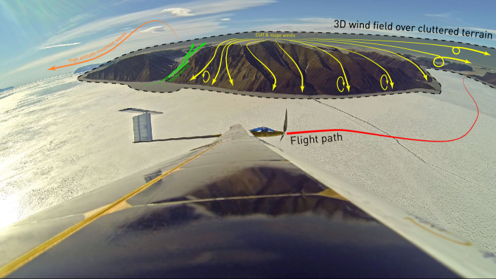
Figure 1: Cluttered terrain and strong winds pose a significant risk to a UAV. This paper therefore presents a downscaling method to predict the local 3D wind field in real time and a path planner to calculate optimal trajectories with respect to the perceived terrain and the calculated 3D wind field. AtlantikSolar’s flights next to the mountains and strong winds above the Arctic in summer 2017 are a prime application for such a framework.

Safe operations in such environments require three technologies that do not exist on today’s small-scale UAVs: First, a Simultaneous Localization And Mapping (SLAM) system to create a map of the environment, second, a method to predict the local 3D wind field around the UAV, and third, a path planner to calculate an optimal collision-free path with respect to the terrain and 3D wind field. The focus of this paper is on wind field prediction and path planning. Such a system needs to run in real time to react to new terrain information. In addition, to guarantee flight safety at all times, including conditions with a degraded communication link, the system needs to run onboard and be independent from local infrastructure.

The current literature does consider path planning in wind. However, the wind fields are not calculated in real time but are pre-calculated using NWP systems on ground-based computers or supercomputers. The UAV can therefore neither react to weather forecast changes nor to terrain features that were not considered by the NWP system. A comprehensive overview of the current state of the art is given in the respective sections on wind field prediction (Section 2.1) and path planning (Section 3.1).

Contributions

This paper presents a path planning framework which integrates local 3D wind field predictions to guarantee the safe and efficient operation of fixed-wing Unmanned Aerial Vehicles in cluttered terrain. The framework runs in real time on the limited computational resources of the UAV’s onboard computer. The on-board implementation is chosen to guarantee that the framework can generate safe paths at all times, i.e. also in cluttered terrain and during remote missions where the telecommunications link is degraded. Two central research contributions are presented:

• Local 3D wind field prediction: Our downscaling method receives low-resolution NWP data as an input via low-bandwidth data links (e.g. satellite communication) and then leverages potential flow theory to generate a high-resolution 3D wind field close to the UAV. The method is assessed in simulations and with LIDAR wind profiles from Swiss Alpine regions.

• Real-time wind-aware path planning: A sampling-based path planner that plans shortest- or time-optimal collision-free paths in the presence of the predicted non-uniform winds is presented. The planner is based on the Open Motion Planning Library (OMPL). We extend this planner to consider the vehicle dynamics through Dubins aircraft primitives and to speed up the planning via obstacle-aware sampling, heuristics for faster nearest neighbor search and fast collision checking on a pre-processed 2.5D map. The calculation of Dubins airplane paths in non-uniform wind is presented.

This paper is the first in the literature to implement real-time 3D wind field predictions from onboard a UAV. Therefore, we consider this paper initial work on the path towards full onboard weather-awareness and path planning with UAVs. It is not expected that the simple wind field downscaling method can capture all the different flow patterns occuring in complex terrain. From a scientific viewpoint, the paper therefore seeks to assess, first, how accurately our simple method can predict the wind field when running onboard a UAV in real time, and second, what path cost advantages and computational demands wind-aware path planning results in.

The remainder of this paper is organized as follows. Section 2 presents the design, implementation and assessment of the 3D wind field prediction method. Section 3 presents the wind-aware path planning framework and assesses it in synthetic and real-terrain test cases with wind fields generated by our wind downscaling method. Section 4 presents a summary and concluding remarks.

2 Prediction of 3D Wind Fields from a UAV

This chapter investigates the feasibility of predicting the local 3D wind field in high resolution and real time on the limited computational resources of small UAVs. Given that large-scale weather models are too computationally expensive, we instead trade-off, implement and assess downscaling-based methods. It is assumed that the model has access to low-resolution Numerical Weather Prediction data and terrain information as inputs. Its output is used by the path planner of Section 3.

2.1 State of the Art

The current UAV literature does not discuss UAV-based wind predictions, but only in-situ wind measurements: Filtering approaches that fuse the information of an Inertial Measurement Unit (IMU), Global Positioning System (GPS) and airspeed sensor are mostly used [45, 29]. Approaches that estimate the wind vector without an airspeed sensor also exist [43]. In addition, formations of UAVs have been used to cooperatively measure wind fields [30]. To find suitable methods for the online prediction of 3D wind fields from UAVs, downscaling methods that historically come from the fields of meteorology and flow simulation are therefore investigated. In general, these downscaling methods are of three different types:

• Statistical methods use previously measured wind data in a certain region and thereof derive wind expectations for the same region using statistical methods. Given that we aim to predict the wind over unvisited terrain, these methods are not suitable for our application.

• Prognostic models calculate the approximate solution of differential equations describing the Atmospheric Boundary Layer (ABL). They can reproduce small-scale weather effects, but are computationally expensive. ARPS, the Advanced Regional Prediction System [59, 60], has been applied to complex terrain [36, 37, 21, 46] and is freely available. GRAMM, the Graz Mesoscale Model [3], considers mass, momentum, potential temperature and humidity conservation and is often used together with the dispersion model GRAL (Graz Lagrangian Model), e.g. in Oettl [41]. It is free and provides a GUI.

• Diagnostic methods do not have a proper physical background but return a physically consistent wind field with respect to mass or momentum conservation. They are less computationally demanding than prognostic models but cannot predict local effects such as slope winds [47] or the time-dependency of the flow. MATHEW [52, 53] is a diagnostic mass consistent model which adds a potential field to an initial wind field to make it divergence free. The source code of a modified model is available [58]. CALMET [1] additionally models kinematic terrain effects, slope flows and blocking effects and can incorporate observational data at the cost of increased computational cost. The usage of CALMET coupled to NWP data showed a significant improvement with respect to NWP outputs [56, 35]. Software licences are available for free. WindNinja [12] provides two different models: A mass-conserving model which resembles MATHEW, and a mass- and momentum-conserving model that uses commercial computational fluid dynamics software. Near surface winds are improved especially for high-wind events [57]. The software with GUI is available for free.

2.2 Method Selection

Requirements

Based on the overall goal postulated in Section 1, the following specific requirements are derived for the wind prediction framework: It shall

• be able to calculate a sufficiently accurate 3D wind field for an area of $1\,\mathrm{km^{3}}$ (with the UAV at its center) and 25 m grid resolution in less than 30 s calculation time on the UAV’s onboard computer, which we assume corresponds to 10 s on a standard laptop computer.

• have a robust and fully automated execution that does not require any human intervention.

• be usable on UAVs operating remotely or in cluttered terrain where the communication bandwidth to the ground station is limited.

• be modular and easily modifiable.

Model selection

Five different models were traded off against the requirements presented above. First, both ARPS and GRAMM/GRAL were discarded because they violate the computation time constraint, i.e. usually require far more time to guarantee that a numerically stable solution is reached. The mass- and momentum-conserving version of WindNinja is discarded due to computation time disadvantages, too. Of the remaining models, CALMET is considered slower and has a less modular code base. The two remaining models are MATHEW and the mass-conserving WindNinja, which essentially solve the same mathematical problem. Finally, MATHEW is selected because it has a slim and modular source code and can, as shown by Walt [58], solve similar meteorological downscaling problems within the calculation time requirements. In addition, it solves the internal Finite Element Method (FEM) using FEniCS, an open-source library that already provides many different solvers and preconditioners, has both Python and C++ bindings, and supports various grid types.

2.3 Fundamentals

Mathematical derivation

MATHEW calculates the divergence-free wind field $\vec{u}$ from an initial wind field $\vec{u}^{\text{I}}$ (retrieved from a NWP system), a Digital Elevation Model (DEM) and the stability matrix $\bm{S}$. The problem domain $\Omega$ is an open set in 3-dimensional space and its boundaries are the Dirichlet boundary $\Gamma_{\text{D}}$, which covers the open-flow boundary, and the Neumann boundary $\Gamma_{\text{N}}$ defining the terrain (Figure 2).

Figure 2: Computational domain and boundaries of MATHEW on 2D grid: The red lines and dots represent the open-flow boundary whereas blue is used for the terrain. The black dots are the grid points within the domain $\Omega$ and the black lines illustrate the cells.

The central hard constraint enforced by MATHEW is that the resulting $\vec{u}$ needs to be divergence free over the domain $\Omega$, i.e.

$$\nabla\cdot\vec{u}=0\;.$$ (1)

This essentially means that the flow is incompressible. The main soft constraint is that the adjustments between the initial wind field $\vec{u}^{\text{I}}$ and the final wind field $\vec{u}$ shall be minimal. This expresses the assumption that the initial wind field observation $\vec{u}^{\text{I}}$ contains valuable information collected through sensing or a prior model — and is thus to some degree correct (see Section 2.5.1 for a violation of that assumption). Mathematically, MATHEW reduces the accumulated error between $\vec{u}$ and $\vec{u}^{\text{I}}$ over the domain in a least-squares sense by minimizing the functional

$$\pazocal{L}(\vec{u};\lambda)=\int\limits_{\Omega}\left(\frac{1}{2}\bm{S}\left(\vec{u}-\vec{u}^{\text{I}}\right)\cdot\left(\vec{u}-\vec{u}^{\text{I}}\right)+\lambda\nabla\cdot\vec{u}\right)dV\;,$$ (2)

with velocity potential $\lambda$ and stability matrix $\bm{S}$ (explained in the following subsection). The Euler-Lagrange equations for vector functions

$$\frac{\partial\pazocal{L}}{\partial f_{i}}-\frac{d}{dx}\Big{(}\frac{\partial\pazocal{L}}{\partial f_{i}^{\prime}}\Big{)}=0$$ (3)

are applied to Eq. 2 in order to minimize the functional. The problem definition now has the form

$$\vec{u}=\vec{u}^{\text{I}}+\bm{S}^{-1}\nabla\lambda\;.$$ (4)

Note that while the added potential flow field $S^{-1}\nabla\lambda$ in Eq. 4 is vorticity-free, the final wind field $\vec{u}$ can still contain vorticity (for example recirculation behind a ridge) if it is already present in $\vec{u}^{\text{I}}$. Two boundary conditions are now applied: The no-flow through terrain assumption, which translates to $\vec{u}\cdot\vec{n}=0$ where $\vec{n}$ is the normal vector at the terrain, and the assumption of no adjustment of the normal velocities at the open-flow boundaries, which translates to $\lambda=0$. The resulting system of equations is

$$\vec{u} =\vec{u}^{\text{I}}+\bm{S}^{-1}\nabla\lambda \text{in }\Omega$$ (5)

$$\nabla\cdot\vec{u} =0 \text{in }\Omega$$

$$\lambda =0 \text{on }\Gamma_{\text{D}}$$

$$\vec{u}\cdot\vec{n} =0 \text{on }\Gamma_{\text{N}}\;.$$

These equations can be expressed as a Partial Differential Equation (PDE) for the velocity potential $\lambda$ by taking the scalar product with the gradient operator on both sides of the equations of Eq. 5:

$$-\nabla\cdot\left(\bm{S}^{-1}\nabla\lambda\right) =\nabla\cdot\vec{u}^{\text{I}} \text{in }\Omega$$ (6)

$$\lambda =0 \text{on }\Gamma_{\text{D}}$$

$$\left(-\bm{S}^{-1}\nabla\lambda\right)\cdot\vec{n} =\vec{u}^{\text{I}}\cdot\vec{n} \text{on }\Gamma_{\text{N}}\;.$$

Equation 6 is an elliptic PDE. For the transformation into a FEM problem, the first line in Eq. 6 needs to be post-multiplied with a test function $\pazocal{F}$ satisfying its boundary condition ($\pazocal{F}=0$ on $\Gamma_{\text{D}}$) and integrated over the problem domain $\Omega$:

$$-\int\limits_{\Omega}\nabla\cdot\left(\bm{S}^{-1}\nabla\lambda\right)\pazocal{F}\,dV=\int\limits_{\Omega}\left(\nabla\cdot\vec{u}^{\text{I}}\right)\pazocal{F}\,dV$$ (7)

With the use of Green’s Theorem the left-hand side of Eq. 7 evolves to:

$$-\int\limits_{\Omega}\nabla\cdot\left(\bm{S}^{-1}\nabla\lambda\right)\pazocal{F}\,dV =\int\limits_{\Omega}\left(\bm{S}^{-1}\nabla\lambda\right)\cdot\nabla\pazocal{F}\,dV+\int\limits_{\Gamma_{\text{D}}\cup\Gamma_{\text{N}}}\underbrace{\left(\left(-\bm{S}^{-1}\nabla\lambda\right)\cdot\vec{n}\right)}_{=\vec{u}^{\text{I}}\cdot\vec{n}}\pazocal{F}\,dS$$ (8)

$$=\int\limits_{\Omega}\left(\bm{S}^{-1}\nabla\lambda\right)\cdot\nabla\pazocal{F}\,dV+\int\limits_{\Gamma_{\text{N}}}\left(\vec{u}^{\text{I}}\cdot\vec{n}\right)\pazocal{F}\,dS\;.$$

When plugging the result of Eq. 8 into Eq. 7 and rearranging the terms, the so called weak formulation of the problem is derived:

$$\underbrace{\int\limits_{\Omega}\left(\bm{S}^{-1}\nabla\lambda\right)\cdot\nabla\pazocal{F}\,dV}_{a(\lambda,\pazocal{F})}=\underbrace{\int\limits_{\Omega}\left(\nabla\cdot\vec{u}^{\text{I}}\right)\pazocal{F}\,dV-\int\limits_{\Gamma_{\text{N}}}\left(\vec{u}^{\text{I}}\cdot\vec{n}\right)\pazocal{F}\,dS}_{l(\pazocal{F})}\;,$$ (9)

with bilinear form $a(\lambda,\pazocal{F})$ and linear form $l(\pazocal{F})$. The procedure is to now solve for the velocity potential $\lambda$ using the Ritz-Galerkin discretization (for details see Walt [58]), and to finally re-insert $\lambda$ into Eq. 4 to retrieve the final 3D wind field $\vec{u}$.

Stability matrix

The stability matrix is defined as

$$\bm{S}=\begin{pmatrix}\alpha_{\text{h}}^{2}&0&0\\ 0&\alpha_{\text{h}}^{2}&0\\ 0&0&\alpha_{\text{v}}^{2}\end{pmatrix}\;,$$ (10)

where $\alpha_{\text{h}}$ and $\alpha_{\text{v}}$ are weights for the horizontal and vertical component. In contrast to the work by Sherman [52], they are herein defined as $\alpha_{i}^{2}=1/\sigma_{i}^{2}$, where $\sigma_{i}$ are the observation errors or deviations of the observed and desired wind field. The weights $\alpha_{\text{h}}$ and $\alpha_{\text{v}}$ are used to define the stability parameter $\alpha$ as

$$\alpha=\frac{\alpha_{\text{h}}^{2}}{\alpha_{\text{v}}^{2}}=\left(\frac{w}{u}\right)^{2}\;,$$ (11)

where $u$ and $w$ are the magnitudes of the expected horizontal and vertical wind speeds, respectively. Inserting $\alpha$ into the definition of the stability matrix, its inverse becomes

$$\bm{S}^{-1}=c\cdot\begin{pmatrix}1&0&0\\ 0&1&0\\ 0&0&\alpha\end{pmatrix}\;.$$ (12)

Note that the constant factor $c$ can be and is neglected ($c=1$) in [58, 34] because it, first, does not have an effect on the final wind field $\vec{u}$ as during the solution of Eq. 9 $\lambda$ would automatically be scaled by 1/c, and second, it cannot be used to adjust the atmospheric stability. This is however possible using the stability parameter $\alpha$. Sherman [52] assesses multiple test cases and determines a typical value of $\alpha\approx 10^{-4}$. A larger $\alpha$ implies that the wind field is mainly corrected in vertical direction, a smaller one that the correction is principally applied to the horizontal direction.

2.4 Implementation

Architecture

Figure 3 presents the data sources and steps required by our implementation of MATHEW. The framework is implemented in Python with Robot Operating System (ROS) support. The input data are the simulation parameters, a DEM and coarse NWP data (wind profiles around and within the region of interest). The input data is monitored at 0.5 Hz and the model is initialized when the inputs have changed. The grid is generated and the initial wind field $\vec{u}^{\text{I}}$ is calculated by linearly interpolating the coarse NWP data to the vertical layer heights of the high-resolution grid. Afterwards bilinear interpolation is used within each vertical layer to calculate the wind components at each grid point. The mathematical operations described in Section 2.3 are then executed to solve for the velocity potential $\lambda$, which allows to calculate the adjusted wind field $\vec{u}$ by using Eq. 4. This final wind field is published to ROS nodes such as the flight planner (Section 3).

Figure 3: Wind downscaling architecture: Input data changes trigger the wind field downscaling calculation, which then publishes its outputs to ROS and the flight planner.

The decision to implement the architecture of Figure 3 onboard a UAV instead of a ground-based computer is motivated by the requirement to have wind field forecasts available at all times, i.e. even when flying remotely with reduced communication bandwidth to the ground station. The transmitted data volume therefore needs to be minimal. However, even the $1\,\mathrm{km^{3}}$ high-resolution wind field defined in Section 2.2 contains 1681 horizontal grid points with multiple vertical layers. Calculating this wind field on a ground-based computer and transmitting the results via low-speed telemetry links (for example degraded line-of-sight based telemetry or satellite communication) is not possible in real-time. Therefore, an onboard implementation is chosen. The NWP data is provided by the European Consortium for Small-Scale Modeling (COSMO) model [2] at 1–7 km horizontal resolution and up to 80 vertical layers. A ground-based client computer only extracts the NWP data at the specific time and region of interest. Assuming COSMO-1 NWP data, the $1\,\mathrm{km^{3}}$ region of interest then consists of only 9 horizontal grid points with different vertical levels that need to be transmitted via telemetry. Even low-bandwidth links such as the satellite communication link on AtlantikSolar [38] can manage such a bandwidth. The DEM data comes from an octomap [19] that is either preloaded or generated directly onboard the UAV by a vision-based SLAM node [18].

Parameter optimization

The framework’s accuracy and required computation time depend on three critical parameters: The vertical grid point spacing and the preconditioner and solver used by FEniCS. These are optimized by comparing the model to the analytical results for flow around a hemisphere with radius 0.25 m (Figure 4). It is placed at the origin of the domain $[-1,-1,0]\times[1,1,1]$ (in m) with 1 $\nicefrac{{m}}{{s}}$ inflow in positive $x$-direction. $N_{x}=N_{y}=41$ horizontal grid points are used. The stability parameter is $\alpha=1$. While the horizontal spacing is constant, the vertical spacing is not: The vertical position $z$ of a grid point at vertical index $n$ and position $x,y$ is defined as

$$z(x,y,n)=h(x,y)+\big{(}t(x,y)-h(x,y)\big{)}\cdot\gamma(n)\;,$$ (13)

where $h(x,y)$ is the terrain height and $t(x,y)$ is the top vertical domain boundary at the $x,y$ position. The discrete function $\gamma(n)$ needs to be strictly monotonically increasing and fulfill $\gamma(0)=0$ and $\gamma(N_{z})=1$, where $N_{z}$ is the number of vertical grid points. Equidistant, square-root, linear and squared spacing functions $\gamma(n)$ are tested. The error at a location is defined as the length of the difference vector between the model output and the analytic solution. The weighed total error sums up the product of each local error with the ratio between the height of the respective cell and the average cell height of the entire domain. The median weighted error for all vertical spacings is nearly the same, i.e. about 0.005 $\nicefrac{{m}}{{s}}$. For the linear vertical spacing, the weighted errors show a low standard deviation and a low maximum weighted error of only 0.14 $\nicefrac{{m}}{{s}}$. The linear vertical spacing is therefore selected.

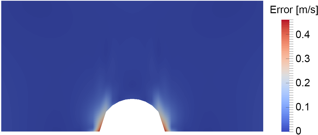
Figure 4: Non-weighted local errors, i.e. the magnitude of the difference between the wind field vectors predicted by the model and the analytical solution, for the hemisphere. The linear vertical spacing, ILU preconditioner and CG solver are used. The largest errors occur in a small region with abrupt terrain change at the bottom of the hemisphere.

The elliptic PDE of Eq. 6 was previously solved [58] using a direct solver. In order to fulfill the stringent computation time requirements, different FEniCS preconditioners and iterative solvers were assessed using the aforementioned hemisphere test case. The best combination is found to be the FEniCS Incomplete LU-decomposition (ILU) preconditioner with the Conjugate Gradient (CG) solver. Averaged over 10 runs, this combination reduces the computation time for $\lambda$ from 81.8 s for the direct solver to only 6.3 s. The calculation time requirements of Section 2.2 are thus fulfilled. The additional errors introduced into the wind field have a norm of less than $10^{-4}\,\nicefrac{\mathrm{m}}{\mathrm{s}}$ and are deemed acceptable given that a time reduction of 92 % is achieved. Figure 4 shows the overall non-weighted errors of the framework. More detailed information on the implementation and parameter optimization is presented by Müller [34].

2.5 Results

2.5.1 Synthetic Test Cases

Steep and narrow valley

The steep and narrow valley (Figure 5) tests how mass conservation is achieved for different stability parameters. At the center of the valley ($x=0$, $y=0$) the width is one fourth of the inflow width. The initial wind field $\vec{u}^{\text{I}}=[5,0,0]\nicefrac{\mathrm{m}}{\mathrm{s}}$ is constant over the entire domain. While $\vec{u}^{\text{I}}$ is divergence free over $\Omega$, it violates the terrain boundary conditions. The model output $\vec{u}$ is shown in Figures 5b and 6. The ratio of the average inflow speed to the average valley wind speed is roughly 1/4, thus mass conservation is fulfilled. However, the average wind speed in the domain is reduced (Table 1) and the expected 20 $\nicefrac{{m}}{{s}}$ within the valley are not reached. For $\alpha=1.00$, the flow is also able to avoid the orifice represented by the valley by rising in front of the valley and sinking again afterwards. Given the open flow boundary above the valley this behavior is expected. Overall, the test case shows that $\vec{u}$ is made divergence free, terrain following and mass consistent. However, it also shows a major drawback of the model: As indicated in Section 2.3, the initial wind field $\vec{u}^{\text{I}}$ is assumed to be a rather close representation of the final flow field. In this case $\vec{u}^{\text{I}}$ inside the valley was however too low by a factor of four. The model does not have a physically-intuitive way to deal with this (e.g. inflow boundary conditions that constrain the problem). Instead it strictly applies Eq. 2 to minimize the total least squares error between $\vec{u}$ and $\vec{u}^{\text{I}}$, which is smaller if $\vec{u}$ is decreased in the inflow than if it is kept constant at the inflow but significantly increased inside the valley.

Table 1: Characteristic wind speeds for the valley test and two stability parameters $\alpha$.

Stability parameter	$\alpha=0.01$	$\alpha=1.00$
Mean valley inflow [m/s]	2.32	2.75
Maximal wind speed [m/s]	11.86	11.55
Average domain wind [m/s]	4.48	4.62

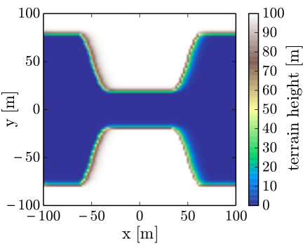
(a)

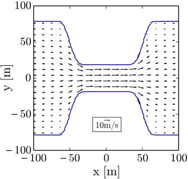
(b)

Figure 5: Synthetic valley. Left: Terrain. Right: Adjusted flow (black arrows) at $z=40\,\mathrm{m}$ and $\alpha=1.00$. As expected, the wind speed in the valley is roughly four times as high as at the in and outflow.

(a)

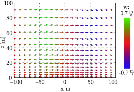
(b)

Figure 6: Adjusted wind fields $\vec{u}$ for $\alpha=0.01$ (left) and $\alpha=1.00$ (right) for the synthetic valley test case in the $x$-$z$ cross section at $y=0$. The arrow color represents the vertical component $w$. As expected, the wind speed is higher inside the valley. The overall wind magnitude is decreased in both cases. For $\alpha=1.00$, the flow is also adjusted vertically.

Ramp

The synthetic ramp test case is also initialized with $\vec{u}^{\text{I}}=[5,0,0]\nicefrac{\mathrm{m}}{\mathrm{s}}$ over the entire domain. The results for the domain heights 160 m and 600 m are visualized in Figure 7. The geometry again represents an orifice for the flow, and the overall wind magnitudes are therefore decreased at the inflow and increased at the outflow. The ratio between inflow and outflow velocities is however lower than in the valley test because the geometry narrows less and the top domain boundary is an open flow boundary where some mass is expelled. The vertical flow field and the regions of maximum wind speed close to the top of the ramp — where soaring flight would be optimal — are represented well. However, differences in the vertical component $w$ above 130 m can be observed: For the domain size of 160 m they are higher and less realistic as the influence of the obstacle should decrease with increasing distance. This is attributable to the fact that the relative sink size (the ratio outflow to inflow) of the initial wind field is much higher for the first case. MATHEW therefore requires a sufficiently large domain height. For the remaining analysis the domain factor, i.e. the ratio of domain height to the height of the tallest obstacle, is therefore set to 3.5. Overall, the results again emphasize that a good initial wind field $\vec{u}^{\text{I}}$ is required. However, in a qualitative sense the results agree very well with the intuitive solution.

(a) Domain height 160 m: 3.85 $\nicefrac{{m}}{{s}}$ average inflow, 5.59 $\nicefrac{{m}}{{s}}$ average outflow, 1.26 $\nicefrac{{m}}{{s}}$ minimal wind, 9.74 $\nicefrac{{m}}{{s}}$ maximal wind.

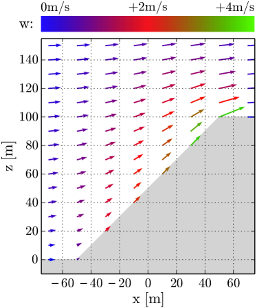
(b) Domain height 600 m: 3.79 $\nicefrac{{m}}{{s}}$ average inflow, 5.79 $\nicefrac{{m}}{{s}}$ average outflow, 1.23 $\nicefrac{{m}}{{s}}$ minimal wind, 9.69 $\nicefrac{{m}}{{s}}$ maximal wind.

Figure 7: Results for the synthetic ramp test case: Both the observed flow acceleration and the vertical components $w$ correspond well to an intuitive solution. The arrows scale with the magnitude and the color visualizes $w$.

2.5.2 Experimental Validation

Measurement and simulation setup

To compare the model output to actual wind data, an extensive literature review for measured multi-dimensional wind fields in complex terrain and at typical flying altitudes of a UAV was performed. Unfortunately, even after multiple weeks of searching no such measurements could be found. Therefore, 1-D LIDAR measurements of wind vectors at multiple altitude levels are used. Figure 8 visualizes an exemplary LIDAR profile. The LIDAR data was recorded by the Zurich University of Applied Sciences at three different locations and time periods (Table 2). It was filtered and averaged to exclude invalid raw data, missing measurements, or excessive changes within consecutive time steps. More details about the exact instrumentation and measurements can be found in [28] and [17] for San Bernardino/Bivio and Vorab, respectively.

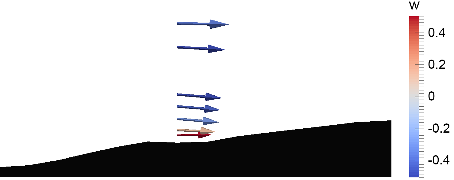
Figure 8: An exemplary LIDAR profile from Vorab, with the arrows representing wind vectors at different heights. While we’d expect $w>0$ due to the left-to-right winds and the increasing terrain altitude in that direction, the LIDAR measurements show $w<0$ for most altitudes. Such unintuitive LIDAR measurements occur regularly. They are often caused by terrain or effects that lie outside the computational domain (e.g. large-scale mountain-waves), which the downscaling model can of course not take into account.

Table 2: LIDAR measurement sites in Switzerland, time periods and amount of valid data (in days and valid LIDAR profiles). The days with valid data are less than the time period because data had to be filtered out e.g. when clouds decreased the data quality.

Site	Lat. ∘N/ Lon. ∘E	Year	Period	Valid data
San Bernardino	46.46357 / 9.18465	2015	Jun.2–Jun.17	2 days/30 prof.
Bivio	46.46251 / 9.66864	2015	Jun.17–Jul.21	2 days/36 prof.
Vorab	46.87398 / 9.18186	2016	Mar.22–Apr.4	6 days/70 prof.

Figure 9 visualizes the terrain, the computational domain and the LIDAR, which is always positioned at the center of the computational domain with side length 2.2 km. A grid with 20 vertical layers and 50 m horizontal resolution is used. Note that for San Bernardino and Bivio only COSMO-2 weather data is available, while the higher-resolution COSMO-1 data can be used for Vorab.

(a) San Bernardino

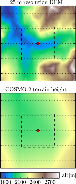
(b) Bivio

(c) Vorab

Figure 9: Terrain (5x5 km), downscaling domain (2.2x2.2 km, dashed line) and LIDAR locations (red diamond). North is up. The COSMO-2 terrain is not able to resolve the cluttered terrain in San Bernardino and Bivio. The initial wind field $\vec{u}^{\text{I}}$ provided by COSMO-2 will thus not be a good approximation for $\vec{u}$. The COSMO-1 terrain represents the terrain at Vorab better. DEM data: © 2016 swisstopo (JD100042), free for educational purposes.

Measured and estimated wind fields

To show how the downscaling model can improve the wind field estimate, but to also show its limitations with respect to modelling small-scale thermally induced wind phenomena, this section exemplarily compares the model output and measured winds for Bivio. As visible in Figure 9b the LIDAR is located in a steep east-west valley but the corresponding COSMO-2 terrain is basically flat. As a result, on July 8th 9:00 UTC the interpolated COSMO-2 wind field indicates flow coming from south-east (Figure 10) and therefore violates the assumption of no flow through the terrain boundaries. The downscaling model is able to rotate $\vec{u}$ in the correct direction such that the winds satisfy the terrain boundary conditions. The measured wind direction agrees well with the downscaled wind field. However, the wind speed is significantly underestimated both by the initial wind field and the adjusted wind field. The overall observed situation is a so called mountain breeze, i.e. a cold air mass that moves from the mountain into the valley during the night and early morning hours.

(a)

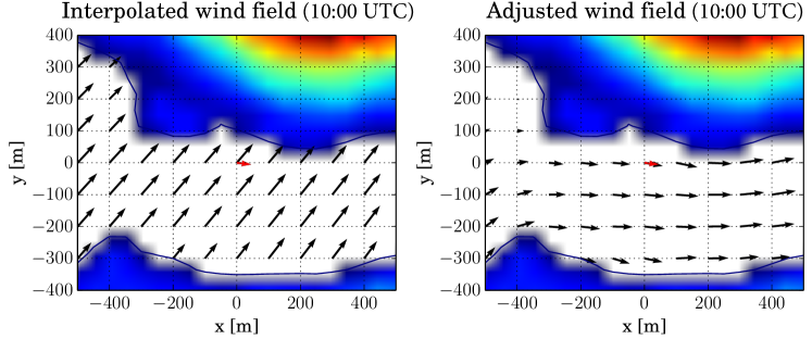
(b)

Figure 10: Initial and adjusted wind fields $\vec{u}$ (black arrows) at Bivio for 09:00UTC (top) and 10:00UTC (bottom) on July 8th 2015. The wind is shown at 1900 m AMSL. The red arrow is the wind measured by the LIDAR.

One hour later, at 10:00 UTC, the wind direction has changed and wind is flowing from the valley to the mountains. This valley breeze situation is shown in Figure 10. The interpolated wind direction again does not respect the terrain boundaries and also differs significantly from the measured wind direction. The downscaling model is again able to predict the correct wind direction. The wind magnitude is overestimated by both approaches, but the error for the downscaling model is much smaller.

To analyze the reason for the underestimated wind speed at 09:00 UTC, Figure 11 plots the measured, interpolated and modeled wind profiles. The measured horizontal wind profile shows a distinct maximum 40 m above ground. This small-scale phenomenon is called low-level jet and is not represented in the interpolated wind profile. Given that the downscaling model has no deeper physical understanding of thermally-induced effects, it also cannot predict this behavior. At 10:00 UTC, the interpolated wind is again too high but the downscaling model can partially correct for this. In both cases, the downscaling model clearly improves the wind direction such that the overall agreement between the modeled and measured wind vectors is improved.

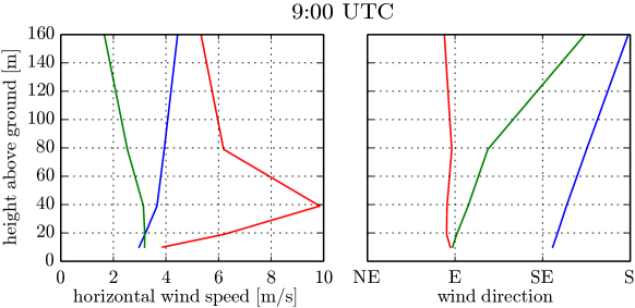
(a)

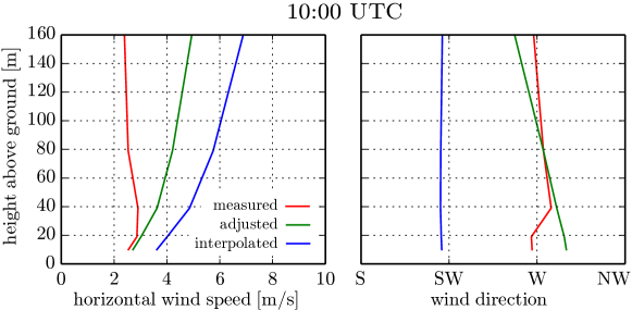
(b)

Figure 11: Wind profiles at Bivio on July 8th 2015 at 9:00 UTC (top) and 10:00 UTC (bottom). In the top plot, the LIDAR measures a so-called low-level jet. The downscaling model significantly improves the wind direction and tends to improve the wind speed.

Statistical evaluation

To quantitatively assess the wind field improvement, a comparison of the downscaling model against LIDAR measurements is performed over all test cases. Given that we only want to investigate modeling errors but not errors due to a badly selected stability parameter, we always first run the model for $\alpha=[10^{-6},10^{1}]$ and select the run with the optimal $\alpha$, i.e. the one which yields the minimum Root Mean Square Error (RMSE) between the modeled and measured wind profile. This approach of course has a certain risk of overfitting such that the following results have to be considered best-case results. In the future, the wind field downscaling model will automatically select the best $\alpha$ by assessing the current atmospheric stratification using the temperature profiles in the NWP data.

Given that only 1D measurement data exists, all wind fields can only be compared locally at the LIDAR’s position. In addition to the downscaled wind field $\vec{u}$, we also compare the initial wind field $\vec{u}^{\text{I}}$ and a zero-wind field $\vec{u}^{0}=0$. The LIDAR measurements serve as ground-truth. The comparison metric is the root mean square error. It is calculated for two newly introduced variables: First, the weighted horizontal vector error is

$$e_{\text{hor}}=\frac{\sqrt{(u_{\text{p}}-u_{\text{m}})^{2}+(v_{\text{p}}-v_{\text{m}})^{2}}}{v_{\text{air}}}\;.$$ (14)

Here, the subscripts p and m stand for the predicted and measured components, and $v_{\text{air}}$ is the nominal airspeed of 9 $\nicefrac{{m}}{{s}}$ for AtlantikSolar. The variable $e_{\text{hor}}$ therefore normalizes the horizontal wind estimate error with the aircraft speed. If $e_{\text{hor}}>1$, the wind is too strong to overcome the wind and collision with terrain can occur. The second variable is the weighted vertical error

$$e_{\text{ver}}=\begin{cases}\frac{w_{\text{p}}-w_{\text{m}}}{w_{\text{sr}}}&\textnormal{if }w_{\text{p}}-w_{\text{m}}\leq 0,\\ \frac{w_{\text{p}}-w_{\text{m}}}{w_{\text{cr}}}&\textnormal{if }w_{\text{p}}-w_{\text{m}}>0\;,\end{cases}$$ (15)

where $w_{\text{sr}}$ is the maximum sink rate (positive) and $w_{\text{cr}}$ the maximum climb rate. For AtlantikSolar these are 3 $\nicefrac{{m}}{{s}}$ and 1.5 $\nicefrac{{m}}{{s}}$ respectively. This error is especially important for fragile or low-power aircraft: For example, if the predicted vertical wind $w_{\text{p}}=0\,\nicefrac{\mathrm{m}}{\mathrm{s}}$ and $e_{\text{ver}}<-1$, then the aircraft sink rate is exceeded when altitude hold is required and the aircraft may get damaged. Equivalently, when $w_{\text{p}}=0\,\nicefrac{\mathrm{m}}{\mathrm{s}}$ but $e_{\text{ver}}>1$, then the actual downwards wind magnitude is higher than the aircraft climb rate and the aircraft is in risk of colliding with terrain. Overall, if any of the error magnitudes exceed unity, the aircraft is in danger.

Table 3 shows the final results. The root mean square horizontal errors, vertical errors, and — given that they were already properly normalized with the aircraft nominal speed, climb rate and sink rate — their sum are presented. In Bivio, the vertical error is reduced by neither the initial nor the downscaled wind field but the horizontal error is reduced by 38 % by the downscaling model. In San Bernardino, the vertical error is slightly reduced by both $\vec{u}^{\text{I}}$ and $\vec{u}$. The horizontal error is reduced by 27 % by $\vec{u}^{\text{I}}$ and by 31 % by $\vec{u}$. In Vorab, the initial wind field yields a much larger vertical error than the zero-wind assumption and the downscaling model can only marginally compensate for that. The horizontal error is however reduced by 46 % by $\vec{u}^{\text{I}}$ and by 48 % by $\vec{u}$. Averaged over all three test cases (with equal weight for each), it becomes clear that both COSMO-2 and the higher-resolution COSMO-1 model provide initial wind fields which have similar or higher vertical errors than the zero-wind assumption. The low-quality terrain representation (Figure 9) is certainly contributing to this issue. The downscaling model then does not have the leverage to significantly improve this: On average, $\vec{u}^{\text{I}}$ increases the vertical error by 30 %, and the error increase after downscaling is still 26 %. However, the horizontal error is reduced by 31 % by the initial wind field and by 41 % for the downscaled wind field. The sum of both errors reduces by 15 % with the initial wind field and by 23 % with the presented downscaling method.

The error histograms are displayed in Figure 12. In a first step, only the horizontal error distribution is analysed: The no wind assumption shows a wide distribution with two peaks at approximately 4 $\nicefrac{{m}}{{s}}$ and 12 $\nicefrac{{m}}{{s}}$. The interpolation of NWP data already performs better and the respective error distribution has only one peak at slightly below 4 $\nicefrac{{m}}{{s}}$. The output for the model with optimal stability parameter performs even better, the respective peak is around 3 $\nicefrac{{m}}{{s}}$. Looking at the vertical error distributions, the zero wind assumption leads to the smallest RMSE. The interpolated wind field shows a much higher vertical RMSE and thus more spread in the error distribution. The adjusted wind field shows a very similar distribution. As discussed before, this mainly comes from the measurements in Vorab ($e_{\text{ver}}=$0.713/0.272/0.142 for Vorab/San Bernardino/Bivio respectively), which show vertical winds that cannot be described by simple phenomena (see for example Figure 8) and are therefore not covered in COSMO data. It should be noted that modeling local anomalies such as mountain waves or thermal flows is also very challenging for more complex (e.g. prognostic) downscaling models. In addition it is also possible that the LIDAR data is error-prone because of clouds, fog or precipitation. All in all, the adjusted wind field however has a 23% and 15% smaller RMSE than the zero-wind and interpolated wind fields respectively.

Table 3: Horizontal and vertical wind estimate root mean square errors for the zero-wind assumption $\vec{u}^{0}$, the NWP-based interpolation $\vec{u}^{\text{I}}$ and the adjusted wind field $\vec{u}$ with optimal stability parameter. The LIDAR measurement serves as wind ground truth. The percentage values are the relative changes with respect to the zero-wind assumption.

Type	RMSE($e_{\text{ver}}$)	RMSE($e_{\text{hor}}$)	Sum
Bivio
Zero wind	0.130	0.541	0.671
Interpolated wind	0.159 (+22%)	0.522 (-4%)	0.681 (+1%)
Optimal adjusted wind	0.142 (+9%)	0.339 (-38%)	0.481 (-28%)
San Bernardino
Zero wind	0.299	0.713	1.012
Interpolated wind	0.268 (-10%)	0.517 (-27%)	0.785 (-22%)
Optimal adjusted wind	0.272 (-9%)	0.493 (-31%)	0.765 (-24%)
Vorab
Zero wind	0.466	1.200	1.666
Interpolated wind	0.737 (+58%)	0.643 (-46%)	1.380 (-17%)
Optimal adjusted wind	0.713 (+53%)	0.627 (-48%)	1.340 (-20%)
All test cases combined
Zero wind	0.298	0.818	1.116
Interpolated wind	0.388 (+30%)	0.561 (-31%)	0.949 (-15%)
Optimal adjusted wind	0.376 (+26%)	0.486 (-41%)	0.862 (-23%)

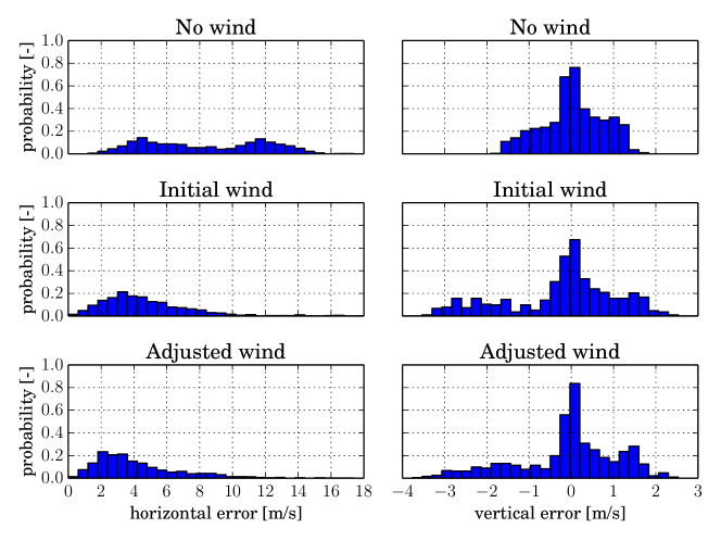
Figure 12: Error histograms: The horizontal error distribution is clearly improved by the downscaling model, but the vertical component is worse than the no wind assumption.

3 Real-Time Wind-Aware Path Planning for UAVs

This section presents a wind-aware path planner that runs in real time on a UAV’s onboard computer and incorporates the real-time 3D wind field predictions from Section 2. It uses near-optimal Dubins aircraft paths to represent the vehicle dynamics and terrain information from a SLAM system to generate safe and efficient paths through wind and cluttered terrain. This section presents the state of the art, fundamentals, improvements for fast shortest-path planning (Section 3.4), the wind-aware time-optimal planning (Section 3.5), and overall results (Section 3.6).

3.1 State of the Art

Motion planning can be performed using grid-based approaches [16], Artificial Potential Fields [26] or sampling-based methods. Rapidly-exploring Random Trees (RRT) [31] are a well-known non-optimal sampling-based planning technique for high dimensional problems or vehicles with nonholonomic constraints. The non-optimal RRT has been extended with the asymptotically optimal RRT* [23]. Other optimal sampling-based planners include BIT* [15], PRM* [24], or FMT* [22]. Gammell et al. [14] introduce IRRT*, a planner that uses information from already known solutions to improve the convergence to the optimal path. Sampling-based planners have been applied to time-optimal planning in uniform wind by Ceccarelli et al. [7], Hota and Ghose [20], and Schopferer and Pfeifer [51]. The extension, time-optimal planning in non-uniform wind, is presented by Lawrance and Sukkarieh [32] and Otte et al. [42]. The approach presented by Chakrabarty and Langelaan [8] is able to compute the time-optimal path in non-uniform time-varying wind fields. In previous work [39] we have presented a similar approach that plans optimal paths considering extensive non-uniform time-varying weather data, but does not run in real time. To our knowledge, no approach that can plan cost-optimal aircraft paths in non-uniform 3D wind fields in real time has been demonstrated.

3.2 Fundamentals

Motion planning is the problem of finding a path from start state $q_{\text{start}}\in Q_{\text{free}}$ to the goal configuration $q_{\text{goal}}\in Q_{\text{free}}$ through the free space $Q_{\text{free}}={Q\setminus Q_{\text{obs}}}$ while obeying additional constraints (e.g. vehicle dynamics). Here, $Q$ is the set of all possible robot configurations and $Q_{\text{obs}}$ is the set of robot states that are infeasible e.g. due to obstacles. While the states can be selected using grid-based approaches [16], this paper focuses on sampling-based planning methods and more specifically the asymptotically optimal RRT* [23] and its informed counterpart IRRT* [14].

3.2.1 Sampling-Based Path Planning Methods

RRT*

Sampling-based planners are advantageous because their computational complexity stays manageable for higher-dimensional problems and $Q_{\text{free}}$ does not have to be constructed explicitly. Such planners are probabilistically complete, i.e. are guaranteed to find a solution if one exists and infinite time is available. RRT* is also asymptotically optimal, i.e. the path converges to the optimal path over time. Algorithm 1 contains pseudo-code for RRT*. After initialization of the motion tree $T$, such planners randomly select a configuration $q_{\text{rand}}$ from $Q$. The current configuration $q_{\text{nearest}}\in T$ which has the smallest distance to $q_{\text{rand}}$ is then found. The actual new state $q_{\text{new}}$ is then selected such that it lies on the path between $q_{\text{rand}}$ and $q_{\text{nearest}}$ and is no further than $d_{\text{max}}$ away from $q_{\text{nearest}}$. This capping step in the so-called steering function avoids excessively long path segments in $T$ because they have a higher probability of collision and therefore yield only few valid motions. Next the motion from $q_{\text{nearest}}$ to $q_{\text{new}}$ is checked for validity, meaning that it does not collide with any obstacle. If that is the case, then either the $k$-nearest neighbors of $q_{\text{new}}$ or all states within a distance $r$ from $q_{\text{new}}$ are determined and stored in $Q_{\text{near}}$. The values of $k$ and $r$ are dependent on the number of nodes in the motion tree $n$:

$$k =k_{\text{rrg}}\ln\left(n\right)$$ (16)

$$r =\sqrt[\text{dim}]{r_{\text{rrg}}\frac{\ln(n)}{n}}\;,$$ (17)

where $k_{\text{rrg}}$ and $r_{\text{rrg}}$ are variable parameters and dim is the dimension of the state space. The neighbor in $Q_{\text{near}}$ with the lowest cost-to-go to $q_{\text{new}}$ (with respect to a cost function $f_{\text{cost}}$) is selected as parent $q_{\text{parent}}$. The edge from $q_{\text{parent}}$ to $q_{\text{new}}$, which is part of the currently best-known path from $q_{\text{start}}$ to $q_{\text{new}}$, is added to the motion tree $T$ and $q_{\text{new}}$ is added as a vertex. The so-called rewiring step is one of the main differences to RRT as it provides the optimality-properties of RRT*: It checks whether any of the paths from $q_{\text{new}}$ to the elements of $Q_{\text{near}}$ is more optimal than the previously known respective path. If so, then that path is rewired, i.e. the parent of $q\in Q_{\text{near}}$ is set to $q_{\text{new}}$. The RRT* algorithm terminates if the termination condition, e.g. expressed through the number of iterations or a certain error metric, is fulfilled.

Algorithm 1 RRT* Algorithm: A motion tree $T$ is generated from the initial configuration $q_{\text{start}}$ until the terminationCondition is fulfilled.

1:procedure solve

2:     $T$.init$\left(q_{\text{start}}\right)$

3:     while $\left(\textsc{terminationCondition}==\text{false}\right)$ do

4:         $q_{\text{rand}}\leftarrow\textsc{sampleRandomState}\left(\right)$

5:         $q_{\text{nearest}}\leftarrow\textsc{getNearestNeighbor}\left(q_{\text{rand}},T\right)$

6:         $q_{\text{new}}\leftarrow\textsc{Steer}\left(q_{\text{nearest}},q_{\text{rand}},d_{\text{max}}\right)$

7:         if $\textsc{motionValid}\left(q_{\text{nearest}},q_{\text{new}}\right)$ then

8:              $Q_{\text{near}}\leftarrow\textsc{getNeighbors}\left(q_{\text{new}},T\right)$

9:              $q_{\text{parent}},\text{cost}\leftarrow\textsc{getBestParent}\left(q_{\text{new}},Q_{\text{near}},f_{\text{cost}}\right)$

10:              $T$.add_edge$\left(q_{\text{parent}},q_{\text{new}},\text{cost}\right)$

11:              $T$.add_vertex$\left(q_{\text{new}}\right)$

12:              $\textsc{rewireTree}\left(q_{\text{new}},Q_{\text{near}},f_{\text{cost}}\right)$

13:         end if

14:     end while

15:end procedure

Informed RRT*

The Informed RRT* algorithm [14] proceeds exactly like RRT* until a first feasible path is found. After that, it leverages the information on the initial solution to speed up the convergence towards an optimal solution: First, it only samples the informed subset $Q_{\text{inf}}$, i.e. the solutions which are known to be able to improve the solution:

$$Q_{\text{inf}}=\{q\in Q|h(q)\leq c_{\text{best}}\}\;.$$ (18)

Here, $c_{\text{best}}$ is the cost of the current best solution and $h(q)$ is a heuristic function which returns a lower limit for the cost of a path from start $q_{\text{start}}$ to goal $q_{\text{goal}}$ which is constrained to go through $q$. As an example, for shortest-path planning problems in $\mathbb{R}^{n}$ the Euclidean distance is a valid heuristic such that the informed subset becomes

$$Q_{\text{inf}}=\big{\{}q\in Q\big{|}\|q_{\text{start}}-q\|_{{}_{2}}+\|q_{\text{goal}}-q\|_{{}_{2}}\leq c_{\text{best}}\big{\}}\;.$$ (19)

This informed subset is an $n$-dimensional prolate hyperspheroid (a special form of a hyperellipsoid) with focal points $q_{\text{start}}$ and $q_{\text{goal}}$. For simple cases such as an ellipsoid, states from the informed subset are sampled directly [14]. For more complicated cases such as general cost functions or differential constraints, indirect sampling based on rejecting all samples $q\not\in Q_{\text{inf}}$ has to be used. Given that this process becomes very inefficient for high-dimensional problems, Kunz et al. [27] propose the hierarchical rejection sampling method. Second, Informed RRT* performs tree pruning, i.e. after a new solution is found all states in the motion tree $T$ that cannot improve the solution anymore are removed. Overall, the combination of informed sampling and tree pruning significantly speeds up the planner’s convergence.

3.2.2 Dubins Airplane Paths Without Wind

The Dubins path [11] is the shortest path between two states in an obstacle-free world for a car which can only drive forward at constant velocity and turn at a bounded turning rate. The shortest path consists of three segments which are either straight (S), left turn (L), or right turn (R) with the maximum turn rate. Six optimal maneuvers exist: RSR, LSL, RSL, LSR, RLR, LRL. For certain cases, the classification scheme by Shkel and Lumelsky [54] can determine the optimal maneuver type without explicitly computing the length of all six maneuvers. The Dubins airplane [9] is the extension of the Dubins car to 3D. The aircraft state $q$ is subject to the dynamics

$$\dot{q}=\begin{bmatrix}\dot{x}\\ \dot{y}\\ \dot{z}\\ \dot{\psi}\end{bmatrix}=\begin{bmatrix}v_{\text{air}}\cdot\cos(\gamma)\cdot\cos(\psi)\\ v_{\text{air}}\cdot\cos(\gamma)\cdot\sin(\psi)\\ v_{\text{air}}\cdot\sin(\gamma)\\ u_{\psi}\end{bmatrix}\;,$$ (20)

where $x$, $y$, and $z$ represent the position and $\psi$ the heading. The aircraft airspeed $v_{\text{air}}$ is assumed to be constant. The two inputs of the system are the path angle (climb and sink angle) $\gamma$ and the turn rate $u_{\psi}$. The inputs are subject to the constraints

$$\gamma \in\big{[}-\gamma_{\text{max}},\gamma_{\text{max}}\big{]}\;,$$ (21)

$$u_{\psi} \in\big{[}-\frac{g}{v_{\text{air}}}\cdot\tan\left(\phi_{\text{max}}\right),\frac{g}{v_{\text{air}}}\cdot\tan\left(\phi_{\text{max}}\right)\big{]}\;,$$ (22)

where $\gamma_{\text{max}}$ is the maximum allowed path angle, $g$ the gravitational acceleration, and $\phi_{\text{max}}$ the maximum allowed bank angle. The bank angle limit can also be expressed in terms of the aircraft’s minimum turn radius

$$r_{\text{turn}}=\frac{v_{\text{air}}^{2}}{\tan\left(\phi_{\text{max}}\right)\cdot g}\;.$$ (23)

The Dubins airplane path is the shortest path under these dynamics between two states in an obstacle-free environment without wind. The calculation method [9] relies on projecting the start and goal states into a horizontal plane, solving the respective Dubins car problem, and then expanding the path back to three dimensions by computing the climbing angle and adding a climb/sink helix if necessary. The so called low- and high-altitude Dubins airplane paths are calculated optimally. However, no closed-form solution for the medium altitude case exists. To speed up the planning, this paper therefore uses the approximation described in [50] for the $<5\%$ medium altitude cases that occur in usual planning problems. The error with respect to the optimal solution is bounded, but strictly speaking, not all Dubins airplane paths are optimal. More generally, standard Dubins airplane paths have two main limitations: First, they are only a very rough approximation of the aircraft dynamics because the discontinuities in the turn rate make them dynamically infeasible. Scheuer and Laugier [49], Richter et al. [48], or Askari et al. [6] therefore present the generation of curvature continuous paths. Second, they are only valid in zero-wind. However, McGee et al. [33] extend them to uniform wind, and Section 3.5.1 extends McGee’s work towards Dubins airplane paths for non-uniform wind.

3.3 Implementation and Testing Setup

The path planning framework is implemented in C++ and is deeply integrated with the Robot Operating System (ROS), which provides the interfaces to load the octomap [19] or DEM and the wind field data from the downscaling method described in Section 2. The planning framework is based on and extends OMPL [55]. A variety of planners, among them RRT*, FMT*, PRM* and the informed planners IRRT* and BIT*, is supported. The path’s waypoints are exported to a MAVLink compatible autopilot via Mavros. The whole framework, including generation and processing of its inputs and waypoint outputs, can therefore be tested in a Hardware-in-the-loop simulation using Gazebo/RotorS [13] (Figure 13). In the following sections, the planning performance is assessed with an Intel i7-6500U dual-core processor with 16 GB RAM using the OMPL benchmarking tools. If not mentioned otherwise, each test case is run 100 times with the aircraft and planning parameters in Table 4. More details on the implementation and parameters are presented by Achermann [4].

Table 4: The default parameters used for the planner benchmarking.

Parameter	Variable	Value
Planner parameters
Planner		RRT*
Maximum planning time		2 s/15 s
Terrain altitude source		2.5D map (height checking)
Obstacle aware sampling		true
Custom nearest neighbor search		true
Pre-evaluated height map		false
Bounding box side length	$s_{\text{bb}}$	30 m (all sides)
Terrain height map resolution	$r_{\text{hm}}$	30 m
Meteo map resolution	$r_{\text{mm}}$	30 m
Max. Dubins motion length	$d_{\text{max}}$	$0.2\cdot\text{map size}$
Airplane parameters
Minimum turn radius	$r_{\text{min}}$	25 m
Maximum climbing/sinking angle	$\gamma_{\text{max}}$	0.15 rad
Airspeed	$v_{\text{air}}$	9.0 $\nicefrac{{m}}{{s}}$

Figure 13: The time-optimal planner running in real time in a HIL simulation: RVIZ (left) and Gazebo/RotorS [13] (right) visualizations. The aircraft (yellow arrow) avoids the Alpine terrain and leverages favorable winds that, as indicated by the black arrows, blow from start (green circle) to goal (red circle) in the lower section of the valley.

3.4 Improving Shortest-Distance Path Planning Performance

This section contributes computational performance improvements for shortest-distance aircraft motion planning with RRT*-like methods. The combined performance improvement is analyzed in Section 3.4.6. Two different test cases in Alpine terrain are used: The Dom mountain range (Figure 14a) with start and goal on opposite sides of the mountain and the Kandertal Low test case (Figure 14c).

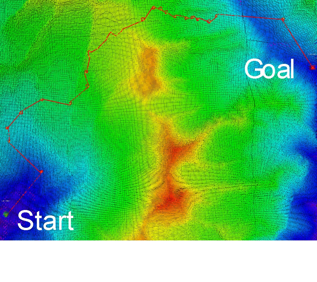
(a) Dom mountain range scenario

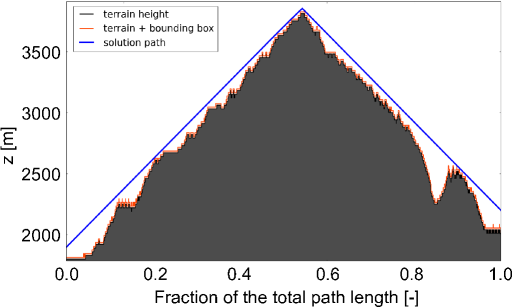
(b) Dom mountain range scenario

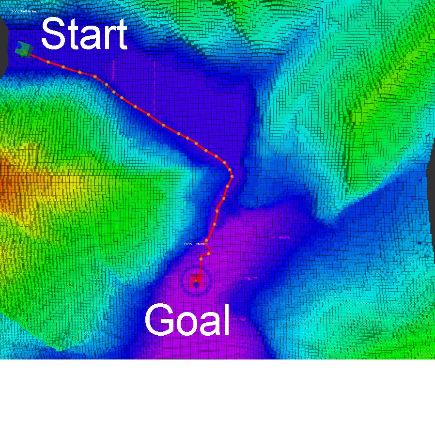
(c) Kandertal Low scenario

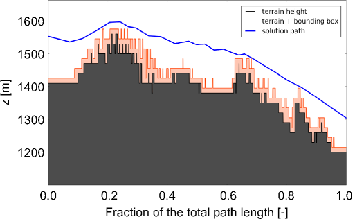
(d) Kandertal Low scenario

Figure 14: The test scenarios with the optimal path after 2 hours of planning. Left: Terrain height (blue equals low terrain, red high terrain) and the path (red). Right: Terrain and path along the total path length fraction.

3.4.1 An Improved Informed Subset for a Dubins Airplane

The Euclidean distance is always shorter than the Dubins aircraft [9] path between two states. It is thus a valid heuristic $h(q)$. However, due to the constrained path angle (and thus climb and sink rate) the aircraft has to fly a helix or lengthen its horizontal path if the goal altitude is too high or low. This fact is used to clip the informed sampling ellipse in $z$-direction. Defining

$$d_{\text{eucl}}(q_{1},q_{2}) =\|q_{1}-q_{2}\|_{{}_{2}}$$ (24)

$$d_{\text{climb}}(q_{1},q_{2}) =\frac{|q_{1}.z-q_{2}.z|}{\sin\left|\gamma_{\text{max}}\right|}\;,$$ (25)

where $q_{1},q_{2}\in Q_{\text{free}}$, then the resulting cost heuristic $h(q)$ for the airplane path length from $q_{\text{start}}$ through $q$ to $q_{\text{goal}}$ is

$$h(q) =\max\big{(}d_{\text{eucl}}(q_{\text{start}},q),d_{\text{climb}}(q_{\text{start}},q)\big{)}$$

$$+\max\big{(}d_{\text{eucl}}(q,q_{\text{goal}}),d_{\text{climb}}(q,q_{\text{goal}})\big{)}\;.$$ (26)

This formulation of $h(q)$ results in the informed subset $Q_{\text{inf}}$ shown in Figure 15. The size of $Q_{\text{inf}}$ is reduced as a function of $\gamma_{\text{max}}$. Of course only informed planners (i.e. IRRT* and BIT* in this framework) benefit from this improved heuristic.

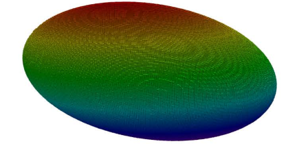
(a)

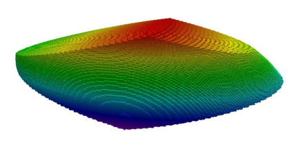
(b)

Figure 15: The left ellipsoid visualizes $Q_{\text{inf}}$ if $h(q)$ is the Euclidean distance only. The right ellipse is the heuristic of Eq. 26, which is capped in positive and negative $z$-direction. Here, a maximum path angle of $\gamma_{\text{max}}=0.25\,\mathrm{rad}$ is used.

3.4.2 Collision Checking

The MotionValid function in Algorithm 1 checks whether a motion lies in $Q_{\text{free}}$. In addition to the initial and final states $q_{1},q_{2}$, all intermittent states are checked by discretizing the motion with the user-specified intermediate collision check distance $d_{\text{icc}}$. This distance should be small enough so that all collisions are detected but large enough to not slow down the motion checking excessively. Our framwork implements both the Flexible Collision Library (FCL) [44] and 2.5D map height checking. For flight at medium to high altitude in outdoor environments, the full 3D collision checking capability of FCL is however not needed. The overhanging geometry of certain obstacles (bridges, power lines, trees) can simply be modeled as 2.5D features to speed up the collision checking.

This paper therefore presents a pre-evaluation method for 2.5D-map based height checking. Standard 2.5D height checking defines the terrain altitude $h_{\text{ter}}(x,y)$ and considers the space below $h_{\text{ter}}$ obstacle space $Q_{\text{obs}}$. The map is then collision-checked against the bounding box of the aerial vehicle. The box size is chosen to fully contain the vehicle in all attitudes. A safety margin for the minimum desired distance to terrain is added. In our implementation, the 2.5D-map is internally always stored at the bounding box resolution. This approach is conservative but efficient because a maximum of four cells of the 2.5D map have to be checked. As shown in Figure 16a, the bounding box can generally intersect with the eight surrounding cells of the current aircraft position. The pre-evaluation calculates the relevant collision area for a cell with center $x_{c},y_{c}$ and any arbitrary aircraft position inside that cell

$$x_{\text{c}}-0.5\left(r_{\text{hm}}+s_{\text{bb}}\right) \leq x\leq x_{\text{c}}+0.5\left(r_{\text{hm}}+s_{\text{bb}}\right)$$ (27)

$$y_{\text{c}}-0.5\left(r_{\text{hm}}+s_{\text{bb}}\right) \leq y\leq y_{\text{c}}+0.5\left(r_{\text{hm}}+s_{\text{bb}}\right)\;.$$ (28)

Here, $r_{\text{hm}}$ is the height map resolution and $s_{\text{bb}}$ is the bounding box side length. The largest $h_{\text{ter}}$ in the relevant area is determined and filled into the corresponding cell of the pre-processed height map (Figure 16b). As a result, instead of checking four cells, only the single cell the aircraft actually is in has to be checked. The downside is that the pre-evaluated collision checking is more conservative, i.e. it effectively increases the bounding box size with a virtual safety margin $\Delta_{\text{sm}}\leq r_{\text{hm}}$.

Figure 16: Left: Standard collision checking with exemplary cell (red) and relevant collision area (orange). Right: Pre-evaluated collision checking with corresponding pre-evaluated cell (red). The numbers represent the terrain height $h_{\text{ter}}$. The figure assumes $s_{\text{bb}}=r_{\text{hm}}$. An exemplary path (red solid line) is shown together with the bounding box swath (red dashed lines) and the cells that need to be checked (grey).

Preliminary results

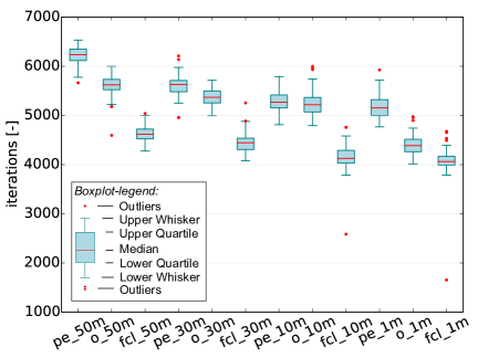
(a) Number of iterations

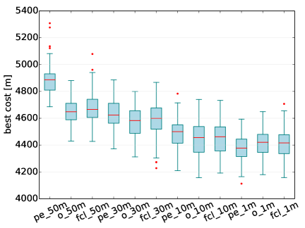
(b) Path cost in meters

Figure 17: Comparison of original 2.5D-map (o_), pre-evaluated 2.5D-map (pe_) and FCL (fcl_) height checking with respect to number of iterations and path cost after 2 s of planning for $r_{\text{hm}}=[1\,\mathrm{m},50\,\mathrm{m}]$ and $s_{\text{bb}}=30\,\mathrm{m}$.

Whereas FCL-based collision checking requires 20–30% of the total planning time, both the original and pre-evaluated height map collision checking require $\leq 0.1\,\mathrm{\%}$ of the planning time for $r_{\text{hm}}\approx s_{\text{bb}}$. Figure 17a plots the number of completed iterations after 2 s of planning in the Kandertal Low scenario. FCL clearly completes the lowest number of iterations. The pre-evaluated height map checking is always faster than the original approach because it only needs to check one cell per planning iteration. The difference is most significant around 1 m map resolution. The result of the increased number of planning iterations on the path cost is shown in Figure 17b. Interestingly, the pre-evaluation only yields better results for $r_{\text{hm}}=1\,\mathrm{m}$. Two separate reasons can be identified: First, the pre-evaluation virtually increases the size of obstacles such that the path around such obstacles has to be longer. While this might not be desired, it is no disadvantage per se because it also makes the path more conservative. Second, the increased obstacle size also leads to more of the sampled states being invalid such that, despite the same number of planning iterations, less valid states can be used for path planning. The overall conclusion is therefore that the pre-evaluated height map should only be used if the height map resolution is small (ca. $r_{\text{hm}}<\frac{1}{30}s_{\text{bb}}$) compared to the bounding box.

3.4.3 Obstacle-Aware Sampling

In Euclidean space, an optimal path generally sticks as close as possible to the straight line path and passes obstacles at small distance. As a result, samples close to obstacles have a higher likelihood to improve the solution path than samples in large open space. Amato [5] presented the idea of obstacle-aware sampling for generic configuration spaces. In this paper we extend Amato’s work by using the specific structure of the aircraft path planning problem, i.e. the fact that start and goal pose are known and the obstacles are represented by a 2.5D map. Let $z_{\text{s,g}}^{\text{min}}=\min(z_{\text{start}},z_{\text{goal}})$ and $z_{\text{s,g}}^{\text{max}}=\max(z_{\text{start}},z_{\text{goal}})$. Then for Dubins airplane shortest-path planning in a 2.5D map, the optimal path always stays above the plane $z=\smash{z_{\text{s,g}}^{\text{min}}}$. The algorithm for obstacle-aware sampling is:

1. Draw a uniform sample $q=(x,y,z,\psi)$ from the state space $Q$ (or from the state $Q_{\text{inf}}$ in the informed case).

2. If $z<z_{\text{s,g}}^{\text{min}}$, resample the $z$-component from a uniform distribution with the boundaries $[z_{\text{s,g}}^{\text{min}},z_{\text{s,g}}^{\text{max}}]$.

3. If $q\in Q_{\text{obs}}$, shift the state $q$ in positive $z$-direction with $\text{dz}_{\text{shift}}$ until $q\in Q_{\text{free}}$. If $q$ is outside the state space $Q$ (for the uninformed case) or the informed subspace $Q_{\text{inf}}$ (for the informed case), return to Step 1.

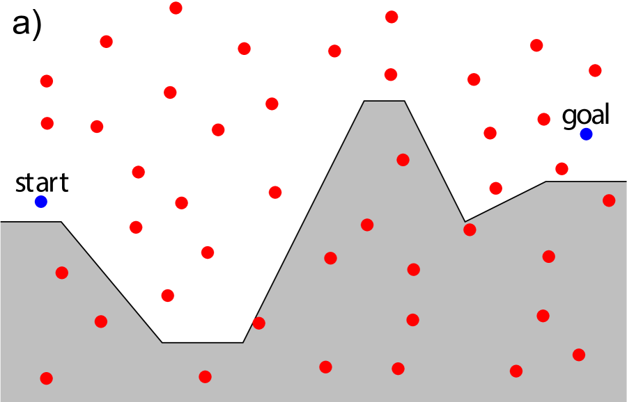
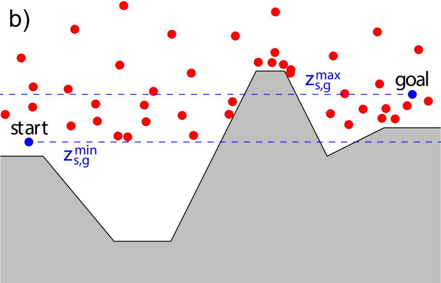
Figure 18: Obstacle unaware (left) and aware (right) sampling. The obstacle-unaware samples are generated over the full map and also inside obstacles. Applying the obstacle aware shifting algorithm results in no states inside obstacles and more states close to terrain.

This sampling approach avoids samples below $z_{\text{s,g}}^{\text{min}}$ which cannot improve the path cost. It increases the sampling density in the regions which contribute most to improving the path cost, i.e. the band between $z_{\text{s,g}}^{\text{min}}$ and $z_{\text{s,g}}^{\text{max}}$, or if this band is fully or partially occupied by terrain, the band with height $\text{dz}_{\text{shift}}$ above the terrain. For example, in Figure 18b there are no samples in the valley but many samples at the top of the hill crest where the optimal path from $q_{\text{start}}$ to $q_{\text{goal}}$ would pass.

Preliminary results

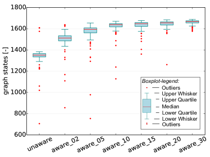
(a) Number of states in the motion tree.

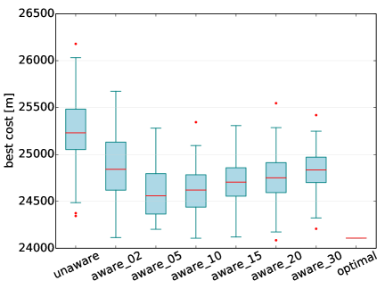
(b) Path cost in meters.

Figure 19: Comparison of obstacle-unaware and obstacle-aware planning (with $k=[2,30]$ given as a postfix) in the Dom scenario after two seconds of planning. The right plot includes the cost after 2 hours of planning (optimal) as a reference.

The iterative $z$-shift is $\text{dz}_{\text{shift}}=k\cdot d_{\text{icc}}$, where $d_{\text{icc}}$ again denotes the intermediate collision check distance and $k$ is a design parameter that is varied for this analysis. The Dom scenario is chosen. Note that due to the significant altitude changes in this scenario, the optimal path consists exclusively of maximum climb or sink rate operation (Figure 14b). As a result, the planner does not chose the most direct path in the horizontal plane (Figure 14a), but could instead choose any path that allows constant maximum climb and sink rate. Figure 19a compares the number of valid states in the motion tree after two seconds of planning. The number of valid states is lowest for obstacle-unaware sampling. It increases asymptotically with $k$ for obstacle-aware sampling. The path costs in Figure 19b clearly show that due to more valid states the obstacle-aware sampling results in lower path costs. The cost errors of the worst configuration (obstacle-unaware sampling) and best configuration (obstacle-aware sampling with $k=5$) to the optimal cost are 1080 m (4.5% error) and 430 m (1.8%) respectively. The error has thus been reduced by more than half, which due to the asymptotic convergence of the planner means that the obstacle-ware planning leads to significantly faster convergence of the solution. For larger $k$ and thus $dz_{\text{shift}}$, the path cost increases again because the shifted samples have a higher distance from the terrain and the path can thus not follow the terrain as closely. The obstacle-aware sampling benefits are high in the Dom scenario because the terrain $Q_{\text{obs}}$ is a significant part of the state space $Q$. Achermann [4] presents further test cases with flatter terrain. Overall, the results suggest to choose $k=[5,10]$.

3.4.4 Nearest Neighbor Search

The nearest neighbor search identifies the closest neighbor or the k-nearest neighbors of a state. RRT* performs each of these computations once per planning iteration. The neighbor search makes up 90 % of the planning time because it involves multiple Dubins path calculations. Two contributions are therefore outlined below.

Speeding up the nearest neighbor search via a Dubins path approximation

When reusing the definitions of $d_{\text{eucl}}$ from Eq. 24 and $d_{\text{climb}}$ from Eq. 25, one can define the Dubins distance approximation

$$\hat{d}_{\text{dubins}}(q_{1},q_{2})=\max\big{(}d_{\text{eucl}}(q_{1},q_{2}),d_{\text{climb}}(q_{1},q_{2})\big{)}\;.$$ (29)

Computing $\hat{d}_{\text{dubins}}$ is around ten times faster than computing the Dubins distance $d_{\text{dubins}}$ itself. The Dubins approximation can be used to define an upper bound for the actual Dubins distance:

$$d_{\text{dubins}}\leq\hat{d}_{\text{dubins}}+\frac{(4\pi+2)\cdot r_{\text{turn}}}{\cos(\gamma_{\text{max}})}\;,$$ (30)

where $\text{r}_{\text{turn}}$ is the aircraft minimum turn radius. Both $r_{\text{turn}}$ and $\gamma_{\text{max}}$ are fixed aircraft parameters and the term on the right hand side is thus constant. It is derived by considering the worst case difference between Dubins distance and Euclidean distance: When the start and goal position are equal but their heading $\psi$ is offset by 180°, then the path offset is $\left(2\pi+2\right)\cdot\text{r}_{\text{turn}}$. The division by $\cos(\gamma_{\text{max}})$ accounts for climb or sink operations. An additional $2\pi r_{\text{turn}}/\cos(\gamma_{\text{max}})$ needs to be added to the offset because the sub-optimal Dubins airplane path is used for the medium altitude case [50]. The proposed method to compute the nearest neighbors then is:

1. Compute the approximation $\hat{d}_{\text{dubins}}$ from the input state to every state in the motion tree and order them from smallest to largest $\hat{d}_{\text{dubins}}$.

2. For the nearest neighbor search the threshold distance is set to the first distance in the ordered list, i.e. $d_{\text{thres}}=\hat{d}_{\text{dubins}}[1]$. For the k-nearest neighbor search it is set to $\smash{\hat{d}_{\text{dubins}}[k]}$, i.e. the k-th element.

3. Identify the index $i$ of the first element in the list for which

   $$\hat{d}_{\text{dubins}}[i]>d_{\text{thres}}+\frac{(4\pi+2)\cdot r_{\text{turn}}}{\cos(\gamma_{\text{max}})}\;.$$ (31)

4. Compute the actual Dubins distance $d_{\text{dubins}}$ from the input state to all states in the sorted list up to $i-1$ and return the nearest or k-nearest states, i.e. those with the smallest value $d_{\text{dubins}}$.

We expect that the planner’s convergence is sped up because the Dubins distance is only calculated for the first $i-1$ states and not all states in the motion tree. This should apply especially for the late planning stages when the motion tree is large.

Considering Dubins path asymmetry during the nearest neighbor calculation

The standard RRT* in OMPL is only designed for symmetric paths. However, the Dubins airplane path is not symmetric, i.e. the distances $q_{1}\rightarrow q_{2}$ and $q_{2}\rightarrow q_{1}$ are generally not equal. Therefore, the k-nearest neighbors from input state to motion tree (required in the RRT* rewiring step) might differ from the k-nearest neighbors from motion tree to input state (required to initially connect the motion tree to the new input state). However, the standard RRT* planner [23] and its OMPL-implementation only compute a single set of nearest neighbors and thus use a potentially wrong neighborhood. We therefore adapt the OMPL RRT* to compute the k-nearest neighbors in both directions. While this is the correct way for asymmetric motions, it of course requires twice the amount of k-nearest neighbor calculations per iteration.

Preliminary results

Table 5: The nearest-neighbor search test configurations. Dub. means the standard OMPL implementation, which calculates the Dubins path to all neighbors, is used. Dub.Appx. means the Dubins approximation of Eq. 30 is used. The 1-way calculation in a Dubins case always represents the motion from the state to the motion tree.

	Nearest neighbor		k-nearest neighbors
	Method	Direction	Method	Direction
ompl_lin	Dub.	1-way	Dub.	1-way
1way_both	Dub.Appx.	1-way	Dub.Appx.	1-way
2way_both	Dub.Appx.	1-way	Dub.Appx.	2-way
1way_onlyk	Dub.	1-way	Dub.Appx.	1-way
2way_onlyk	Dub.	1-way	Dub.Appx.	2-way

The assessment uses the Kandertal Low scenario and the nearest/k-nearest neighbor search configurations in Table 5: First, the RRT* standard neighbor search method which calculates the Dubins distance to all neighbors but is still called linear in OMPL, and second, the Dubins approximation of Eq. 30. Figure 20a shows the number of iterations completed in 15 s planning time, which generally decreases for the custom neighbor search implementation: While ompl_lin computes the distance from the input state to every state in the motion tree once (complexity $O\left(n\right)$), our custom implementation involves sorting $\hat{d}_{\text{dubins}}$ and thus has complexity $O\left(n\log\left(n\right)\right)$. Hence, the custom implementation is slower although fewer Dubins paths are computed. Nevertheless, as shown in Figure 20b, the path cost tends to improve. The 2way_both and 2way_onlyk configurations decrease the remaining error with respect to the optimal path by 25% because they always select the correct neighborhood and therefore the optimal connection between every state in the motion tree is found. This is not always the case for the standard one-way implementation. Note that Achermann [4] presents further test scenarios. The overall conclusion is that the 2way_onlyk configuration yields the largest improvement and should thus be used.

(a) Number of iterations.

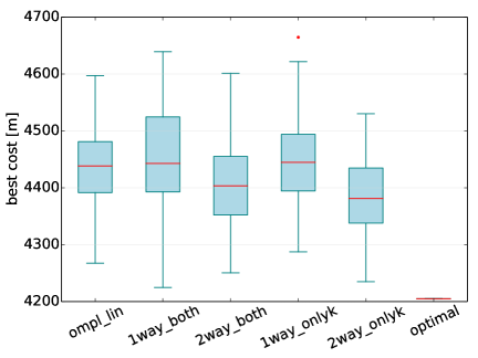
(b) Path length in meters.

Figure 20: Comparison of the OMPL and custom nearest-neighbor search methods in the Kandertal Low scenario after 15 s planning time. The optimal path is shown for reference.

3.4.5 Code Optimization

The Dubins path computation and interpolation is the path planning bottleneck and makes up 80 % of the total planning time. Code optimizations were therefore implemented: First, trigonometric and square-root evaluations for constant angles (e.g. $\gamma_{\text{max}}$) were replaced by pre-computed functions. In addition, trigonometric functions are only evaluated with single instead of double precision, giving a speed up of factor four per evaluation at negligible precision loss (on the order of millimeters). Second, the Dubins path interpolation is improved: The Dubins airplane path consists of at most six segments: Start helix, left/right turn, additional turn in case of the optimal path for the medium altitude case, straight line or left/right turn, another left/right turn, and the goal helix. The segment types, lengths, and climbing angles uniquely define the Dubins airplane path. Previously, for interpolating a state in the $i$-th segment, as required numerous times during collision checking, all previous $i-1$ segments were recomputed. Our implementation calculates the segment ends for a path only once and then caches them for further reuse.

Preliminary results

The performance improvements are evaluated in the Dom, Kandertal Low, and Kandertal High scenarios (where Kandertal High uses the same map as Kandertal Low but a higher-altitude goal state). The number of iterations after two seconds of planning (Figure 21a) increases by around 10 %. The motion tree is therefore also 10 % larger. Due to the asymptotic convergence of the planner, the effect on the path length is much smaller (Figure 21b). The largest performance gain is seen for Kandertal Low where the cost is decreased by about 0.5 percent points (7% of the remaining error to the solution after 2 hours of planning). Nevertheless, the Dubins path interpolation speed up is important because the time-optimal planning of Section 3.5 requires even more Dubins path calculations than the shortest-path planning.

(a) Number of iterations

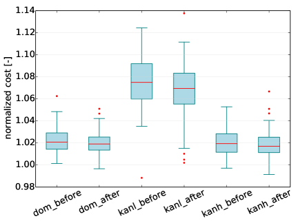
(b) Solution cost after two seconds normalized by the cost after two hours of planning.

Figure 21: Iterations and path cost before and after the code optimization when planning 2 s. The scenarios are Dom (dom_), Kandertal Low (kanl_) and Kandertal High (kanh_).

3.4.6 Performance Results

This section assesses the RRT* planning performance improvements resulting from the features implemented in Sections 3.4.1, 3.4.2, 3.4.3, 3.4.4 and 3.4.5. The selected optimum configuration is a) obstacle-aware sampling with a shifting parameter $k=5$, b) height checking with the original 2.5D map, and c) custom nearest neighbor search only for k-nearest but in both directions. The number of motion tree states after two seconds of planning (Figure 22a) is increased by 30–60 %. Figure 22b shows that the path length errors with respect to the optimal path are reduced from 5.2 to 1.9 percent points (63% reduction), from 10.4 to 7.0 percent points (33% reduction) and from 2.9 to 1.7 percent points (41% reduction) respectively in the Dom, Kandertal low and Kandertal high scenarios. Overall, the error relative to the optimal path is approximately cut in half. Figure 23a shows that a 5% error with respect to the optimal path is reached 10x, 20x and 5x faster than without the optimizations in the Dom, Kandertal Low and Kandertal High scenarios respectively. The presented methods thus significantly improve the planning performance. Figure 23b visualizes the convergence of the planner: For the map sizes, resolution and the non-informed RRT* planner used here, solutions with $<8\%$ error to the optimal solution are on average available after one second and a $<5\%$ error is reached within two seconds. This is a main reason why we consider the framework capable of real-time path planning for a UAV.

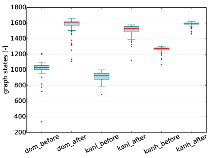
(a) Number of states in the motion tree.

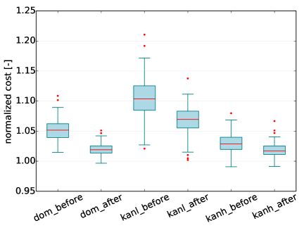
(b) Cost of solution path after two seconds normalized by cost after two hours of planning.

Figure 22: Number of motion tree states and path cost after two seconds of planning time before and after the improvements implemented in this paper. The scenarios are Dom(dom_), Kandertal Low(kanl_), and Kandertal High(kanh_).

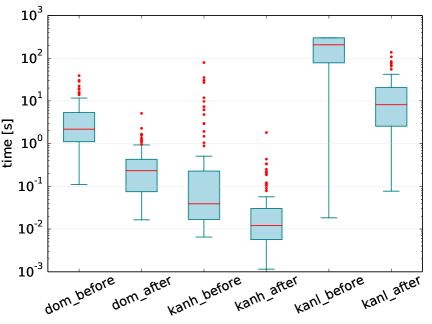
(a) Time required to find a solution at most 5% longer than the path after two hours of planning. The planning time is limited to 300 s.

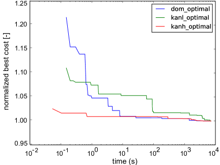
(b) Convergence behavior, i.e. normalized path cost over two hours of planning time.

Figure 23: Performance metrics before and after the implementation of the new methods. The scenarios are Dom(dom_), Kandertal Low(kanl_), and Kandertal High(kanh_).

3.5 Wind-Aware Path Planning

To extend the shortest-path planning to time-optimal planning in 3D wind fields, first, Section 3.5.1 describes the iterative Dubins airplane path calculation in wind. Second, Section 3.5.2 presents the adapted motion cost heuristic. Third, the obstacle-aware sampling of Section 3.4.3 is still partially possible, however, given that in wind the path does not generally fulfill $z>z_{\text{s,g}}^{\text{min}}$ this assumption is removed. Fourth, the standard OMPL neighbor search is used given that Eq. 29 is not valid in wind.

3.5.1 Computing the Dubins Airplane Path in Presence of Wind

Airplane motion planning in wind fields is discussed by numerous authors [7, 42, 8]. McGee et al. [33] present an algorithm to compute the Dubins airplane path for a uniform wind field. Given that this paper also employs Dubins airplane paths, we extend McGee’s approach for spatially varying wind fields. Algorithm 2 presents our iterative approach: First, the Dubins path without wind is computed as described in Section 3.2.2. Second, the resulting path is simulated with wind and the resulting goal pose error due to the wind drift $\smash{\Delta q_{\text{goal}}^{\text{wind}}}$ is determined (Figure 24a). Third, the new shifted virtual goal state $\smash{q_{\text{goal}}^{\text{virt}}=q_{\text{goal}}-\Delta q_{\text{goal}}^{\text{wind}}}$ is determined. The three steps are then repeated iteratively with the new virtual goal state until the ground-relative Dubins path end point and the original goal state have converged to within 1 m Euclidean distance.

Algorithm 2 Computing the Dubins airplane path in spatially-varying wind

1:procedure computeDubinsPathWithWind($q_{\text{start}},q_{\text{goal}},\text{windfield}$)

2:     $q_{\text{goal}}^{\text{virt}}\leftarrow q_{\text{goal}}$

3:     while $\left(\text{converged}==\text{false}\right)$ do

4:         $\text{airpath}\leftarrow\textsc{computeDubinsPathWithoutWind}\left(q_{\text{start}},q_{\text{goal}}^{\text{virt}}\right)$

5:         $\Delta q_{\text{goal}}^{\text{wind}}\leftarrow\textsc{computeWindDrift}\left(\text{airpath},\text{windfield}\right)$

6:         $q_{\text{goal}}^{\text{virt}}\leftarrow\textsc{shiftState}\left(q_{\text{goal}},\Delta q_{\text{goal}}^{\text{wind}}\right)$

7:         $\text{converged}\leftarrow\textsc{isConverged}\left(\text{airpath},\text{windfield}\right)$

8:     end while

9:end procedure

Algorithm 3 describes the wind drift computation. The aircraft position is retrieved through interpolating the air-relative Dubins path and adding the current wind drift. GetWindData determines the wind at the current ground-relative position. The wind drift over the time segment $\Delta t$ is accumulated and the process repeated until the Dubins path is complete. A small $\Delta t_{\text{max}}$ increases the calculation accuracy but also the computation time because more Dubins path interpolations are required (which is why the improvements of Section 3.4.5 are important).

Algorithm 3 Computing the wind drift through numerical integration.

1:procedure computeWindDrift($\text{airpath},\text{windfield}$)

2:     $t\leftarrow 0.0$

3:     $\Delta q_{\text{goal}}^{\text{wind}}\leftarrow\left(0.0,0.0,0.0\right)$

4:     while $t\leq 1.0$ do

5:         $\Delta t\leftarrow\min\left(\Delta t_{\text{max}},1.0-t\right)$

6:         $q_{\text{air}}\leftarrow\textsc{interpolate}\left(\text{airpath},t\right)$

7:         $q_{\text{ground}}\leftarrow q_{\text{air}}+\Delta q_{\text{goal}}^{\text{wind}}$

8:         $\text{winddata}\leftarrow\textsc{getWindData}\left(\text{windfield},q_{\text{ground}}\right)$

9:         $\Delta q_{\text{goal}}^{\text{wind}}\leftarrow\textsc{incrementWindDrift}\left(\Delta t,\text{winddata}\right)$

10:         $t\leftarrow t+\Delta t$

11:     end while

12:     return $\Delta q_{\text{goal}}^{\text{wind}}$

13:end procedure

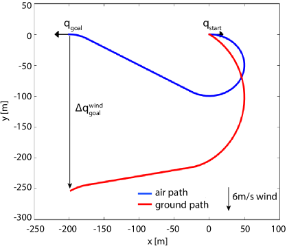
(a) The Dubins path in wind with respect to the ground and air. The wind-induced shift between the end positions of the two paths is $\smash{\Delta q_{\text{goal}}^{\text{wind}}}$.

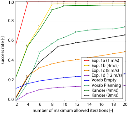
(b) The success rate of computing the Dubins airplane path in presence of wind versus the maximum number of allowed iterations.

Figure 24: Approach and performance of the Dubins airplane path calculation in wind

Preliminary Results

The experimental scenarios conducted to examine the convergence of the Dubins path calculation in the presence of wind are given below. The airspeed is $v_{\text{air}}=9\,\nicefrac{\mathrm{m}}{\mathrm{s}}$. Each experiment is run 100’000 times with random start and goal states.

1. Experiment 1a-d: Wind field of Figure 26b with size 3500 m x 3500 m x 3000 m and wind magnitude a) 1 $\nicefrac{{m}}{{s}}$, b) 4 $\nicefrac{{m}}{{s}}$, c) 8 $\nicefrac{{m}}{{s}}$, and d) 12 $\nicefrac{{m}}{{s}}$.

2. Experiment 2a/b: Vorab region with a 3000 m x 3000 m x 2000 m wind field calculated by the meteo node (Section 2). The maximum wind is 37 $\nicefrac{{m}}{{s}}$, i.e. $v_{\text{wind}}\gg v_{\text{air}}$. Case a) uses uninformed sampling, case b) uses informed sampling such that the start/goal states are closer to each other.

3. Experiment 3a/b: Kandertal region with, for exp. 3a) the same wind field as in exp. 1b), and for exp. 3b) the same wind field as in exp. 1c).

Figure 24b visualizes the percentage of successful Dubins path calculations in wind versus the maximum number of allowed iterations. The success rate increases somewhat asymptotically. In Exp. 1d and Exp. 2a, where $v_{\text{wind}}>v_{\text{air}}$, the success rates stay below 30%. In Exp. 1c and Exp. 3b, where $v_{\text{wind}}$ is only slightly below $v_{\text{air}}$, the success rate increases slowly and only reaches 95% after 100 iterations. Such slow convergence can slow down the overall planner significantly. A maximum number of 12 iterations is therefore chosen. Obviously, finding feasible Dubins paths in strong wind is harder and may even become infeasible at $v_{\text{wind}}>v_{\text{air}}$. McGee et al. [33] explain that for a convergence rate of 1.0 the path may need to be lengthened artificially. Given that, first, this method is not implemented yet, and second, the number of iterations is limited, the optimality property is violated in strong winds and only near-optimal paths are returned.

3.5.2 Motion Cost Heuristic

To allow the use of informed planning and tree pruning in 3D wind fields, the Euclidean motion cost heuristic of Section 3.4.1 needs to be extended: First, the Euclidean distance $d_{\text{eucl}}$ (Eq. 24) between the two states $q_{1},q_{2}$ is computed. Then the maximum components of the wind in $x$-, $y$-, and $z$-direction are determined separately for each axis over the whole wind field. This makes sure that the heuristic is actually a lower bound. The magnitude of this vector projected in the direction of the vector from $q_{1}$ to $q_{2}$ is identified and denoted $v_{\text{wind}}^{\text{proj}}$. Then the time heuristic $h$ is

$$h=\frac{d_{\text{eucl}}}{v_{\text{air}}+v_{\text{wind}}^{\text{proj}}}\;.$$ (32)

Preliminary results

The heuristic must be a lower bound for the actual path cost, but should approximate it as closely as possible such that the heuristic quality $l(q_{1},q_{2})=h(q_{1},q_{2})/c(q_{1},q_{2})\rightarrow 1$. Figure 25 assesses the distribution of the heuristic quality in four different cases: a) zero wind b) uniform 4.0 $\nicefrac{{m}}{{s}}$ horizontal wind, c) uniform 1.0 $\nicefrac{{m}}{{s}}$ vertical wind and d) Exp. 2a from Section 3.5.1. For each setup 1’000’000 different start and goal states are sampled from a 4000 m x 4000 m x 500 m cuboid. The heuristic approximates the zero-wind test case, which is equivalent to a shortest-path problem, best. On average, $l=0.979$. In the time-optimal case, for a vertical wind of 1 $\nicefrac{{m}}{{s}}$ the average quality is $l=0.940$. In the 4.0 $\nicefrac{{m}}{{s}}$ horizontal wind the heuristic quality drops to $l=0.664$, and for the wind field from Exp. 2a it drops to $l=0.189$. The reason is that one small map region has strong wind of 37 $\nicefrac{{m}}{{s}}$. By taking the maximum wind magnitude over the whole wind field, this small region impacts the heuristic over the whole wind field. The very simple heuristic presented here is valid (i.e. $h(q_{1},q_{2})<c(q_{1},q_{2})$) and very fast to compute because it only needs to be calculated once a new wind field is available. It is clearly better than not using a heuristic at all, but it underestimates the cost especially for wind fields with large spatial variations.

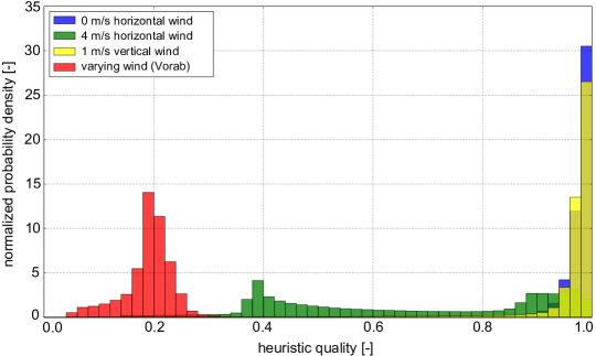
Figure 25: The distribution of the heuristic quality, i.e. the fraction of the motion heuristic divided by the actual motion cost, in four different wind fields.

3.6 Results

The wind-aware and shortest-path planning are compared by running each of them 100 times for 15 s. After each run the planned path is simulated, checked for terrain collisions, and the actual flight time is recorded. Six scenarios that comprise both synthetic test cases and cases with real terrain and wind fields are used:

• w0: No obstacles, horizontal wind of 4.5 $\nicefrac{{m}}{{s}}$ (Figure 26a).

• w1: No obstacles, horizontal wind of 6.0 $\nicefrac{{m}}{{s}}$ (Figure 26b).

• w2: No obstacles, vertical wind with 1 $\nicefrac{{m}}{{s}}$ ( Figure 26c).

• w3: Kandertal low terrain (Figure 14c) with a synthetic wind field that contains horizontal wind of 6 $\nicefrac{{m}}{{s}}$ from $q_{\text{start}}\rightarrow q_{\text{goal}}$ for $z>1850\,\mathrm{m}$ and wind in the opposite direction below this plane.

• vorab 1/2: vorab 1 is the same as Exp. 2a in Section 3.5.1. The maximum wind is 37 $\nicefrac{{m}}{{s}}$ but close to the ground the wind speed is much lower. vorab 2 uses an even stronger wind field with a maximum wind of 59 $\nicefrac{{m}}{{s}}$.

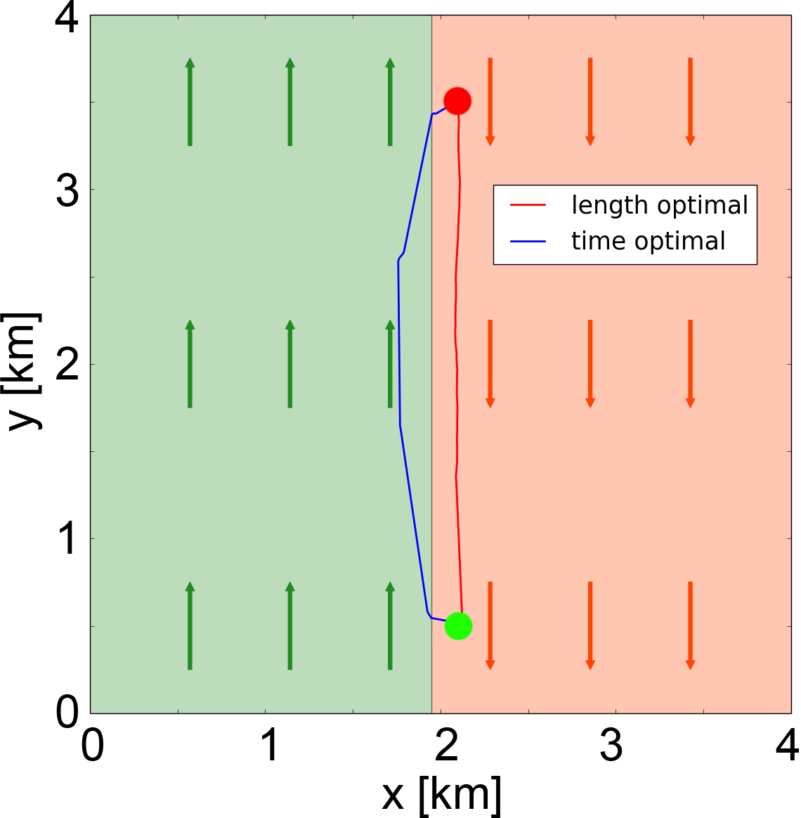
(a) Scen. w0, top down view. 4.5 $\nicefrac{{m}}{{s}}$ wind in the $x$-$y$ plane.

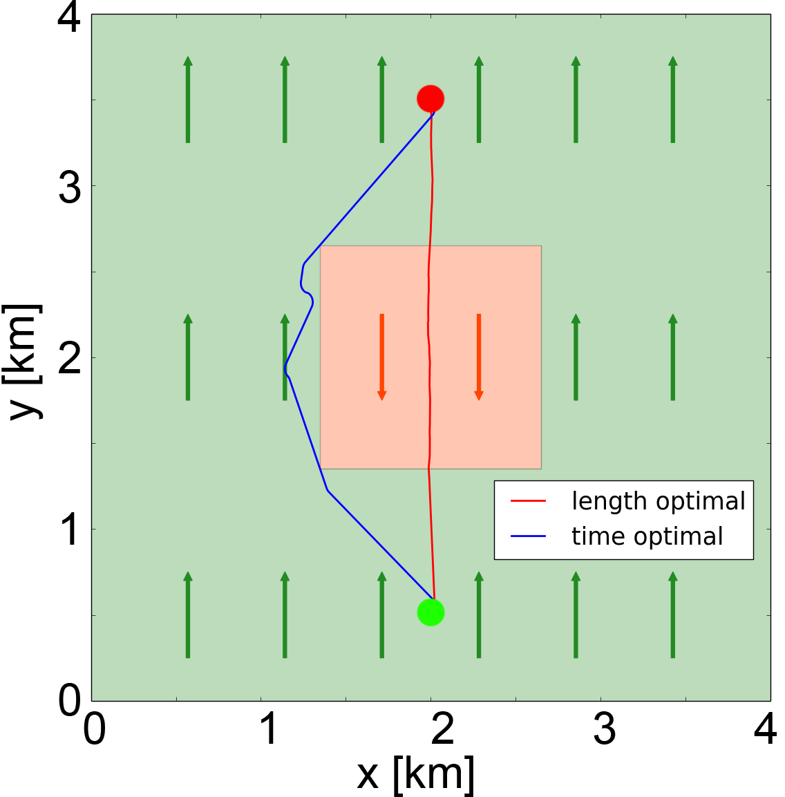
(b) Scen. w1, top down view. 6.0 $\nicefrac{{m}}{{s}}$ wind in the $x$-$y$ plane.

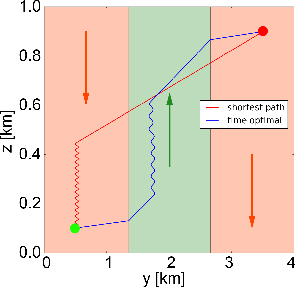
(c) Scen. w2, side view. 1.0 $\nicefrac{{m}}{{s}}$ wind in $z$-direction.

Figure 26: Synthetic test scenarios for planning in wind. The arrows represent wind, the green and red dot start and goal. The shortest and time-optimal path are shown.

Path cost and feasibility

As shown in Figures 26a and 26b, in scenarios w0 and w1 the time-optimal planner always chooses the tailwind areas of the map whereas the shortest-path planner flies through the significant headwind. The time-optimal planner therefore cuts the path cost of the shortest-path planner in half (Figure 28a). Similarly, in scenario w2 shown in Figure 26c, the time-optimal planner optimally leverages the column of rising air to gain altitude more quickly. For real missions this means that the planner can exploit thermal updrafts as described in our previous work [40]. More importantly, as shown in Figure 28b, in scenarios w2 and w3 the time-optimal planner finds feasible paths in 100% of all cases whereas the shortest-path planner does not provide feasible paths at all. The w3 scenario (Figure 27) also clearly shows how the planner leverages favorable horizontal winds: It stays at higher altitude and thus in tailwind longer than the shortest path and thereby reaches its goal in less time. The vorab scenarios show a mixed picture: The shortest-path planner only finds feasible paths in 22% and 68% of all cases for vorab 1 and vorab 2 respectively. The rest of the cases are infeasible and unsafe, i.e. result in collision with terrain due to the neglected influence of the wind. While in vorab 1 the shortest-path planner finds paths with lower cost than the time-optimal planner, these costs are only calculated using the 22% feasible paths. In addition, in vorab 2 the time-optimal planner finds lower cost paths by again actively using the stronger winds at higher altitude.

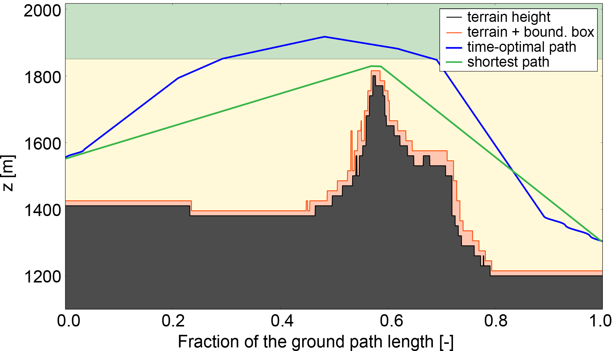
Figure 27: A vertical slice along the path of the w3 scenario. The $x$-axis is the fraction of the ground-relative path length. The winds above 1850 m altitude blow from start$\rightarrow$goal and below that in the opposite direction. The shortest path does not consider this fact, but the time-optimal planner clearly leverages the favorable winds at higher altitude.

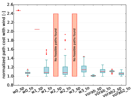
(a) Path cost, i.e. time required to actually fly the path in wind, normalized by the cost of the time-optimal planner after 2 h of planning.

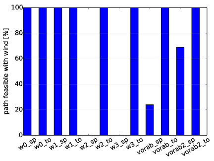
(b) Percentage of feasible paths. Paths are infeasible if the wind causes a terrain collision or if the Dubins path in wind cannot be computed.

Figure 28: The cost and percentage of feasible paths for the time-optimal (_to) and shortest-path (_sp) planner in case of wind. The TO-planner always produces feasible (and thus safe) paths while the SP-planner often causes the aircraft to crash into terrain.

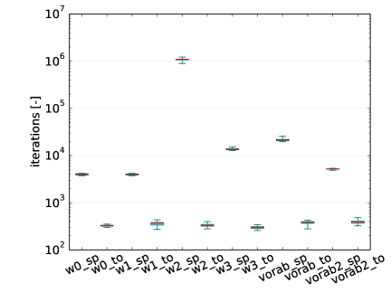
(a) Number of iterations

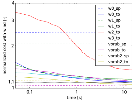
(b) Normalized cost

Figure 29: Number of iterations (left) and cost convergence (right) over 15 s for the time-optimal (_to) and shortest-path (_sp) planners. On the right, the cost is normalized with the time-optimal path cost after two hours of planning. The costs for w0_sp and w1_sp do not converge because the calculated shortest path is not optimal in wind. The results for the w2_sp and w3_sp scenarios are not shown as no valid path was found.

The reason why the feasible shortest paths can be of lower simulated cost than the feasible time-optimal paths is that the time-optimal planning, and particularly the iterative Dubins path calculation in wind, is slow. Figure 29a shows the amount of iterations performed by both planners in 15 s. For the time-optimal planner, the number of iterations is up to 50x lower. As a result, the convergence of the time-optimal planner is much slower (Figure 29b). While the shortest-path planner requires only a couple of milliseconds to converge to below 10% error with respect to the path after two hours of planning, the time-optimal planner needs several seconds. As a result, especially in large maps it may be advantageous to first plan a shortest path and, once more time is available, to then create the wind-aware path.

Influence of the bounding box

Given that many shortest paths result in terrain collisions, it is investigated whether simply choosing a larger bounding box can mitigate the problem. Figure 30a shows the percentage of feasible paths with the shortest-path planning and enlarged bounding boxes. More feasible paths are found and only a slight increase of the solution cost is observed (Figure 30b). Therefore, while no feasibility guarantees for the path can be given, increasing the bounding box size is an efficient way to increase the robustness of the shortest-path planner in wind when the time-optimal planner cannot be used (e.g. on very large maps).

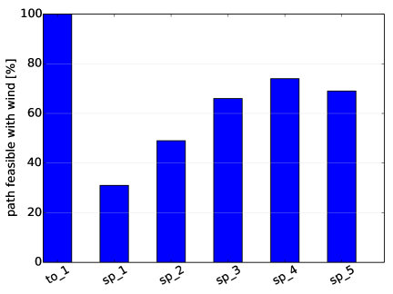
(a) Percentage of feasible paths.

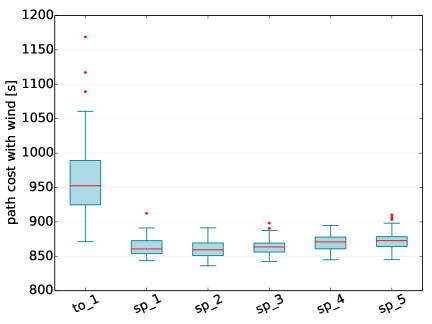
(b) Path cost.

Figure 30: Percentage of feasible paths and path cost with different bounding box sizes in the vorab 1 scenario. The time-optimal (to_) and shortest-path planner (sp_) are run for 15 s. The bounding box side length is a multiple (appendix of the experiment name) of the original bounding box side length.

Effect of the wind magnitude

Figures 31a and 31b show the cost and the fraction of feasible paths for the w0 scenario versus wind magnitudes between 0–8 $\nicefrac{{m}}{{s}}$. Stronger wind results in a lower percentage of feasible paths for the shortest-path planning. The time-optimal planning results in 100 % feasible paths except for when $v_{\text{wind}}\approx v_{\text{air}}$. For 0 $\nicefrac{{m}}{{s}}$ wind speed both planners yield nearly the same cost because the iterative Dubins path calculation already converges after the first run, i.e. it is not more computationally expensive than the non-iterative Dubins calculation in the shortest-path planner. For larger wind speeds more iterations are required, however, the time-optimal planner then also exploits the stronger wind field better. Given sufficient convergence time, the cost advantages of the time-optimal planner increase at higher wind speed. Note that Achermann [4] presents results for the other scenarios which confirm these findings.

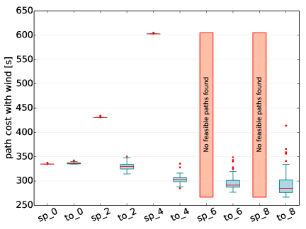
(a) Solution path cost.

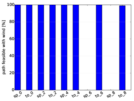
(b) Fraction of feasible paths.

Figure 31: Path cost (left) and feasible paths (right) after 15 s of planning in the w0 scenario for the shortest-path (sp_) and time-optimal planning (to_) and different wind magnitudes. The wind magnitude in $\nicefrac{{m}}{{s}}$ is the number in the experiment name.

4 Conclusion

This paper has presented initial work on a complete real-time environment-aware UAV navigation system: It combines the literature’s first 3D wind field prediction system that runs onboard a UAV and a more standard yet performance-optimized wind-aware path planner. The conclusions and potential future work are summarized below.

3D wind field prediction from onboard a UAV

The onboard 3D wind field prediction is based on downscaling low-resolution wind data from a global weather model. This data is first interpolated to retrieve the initial wind field $\vec{u}^{\text{I}}$. Using simple potential flow theory, $\vec{u}^{\text{I}}$ is adjusted to observe the terrain boundaries in a high-resolution 2.5D height map, mass conservation and the atmospheric stratification. Due to the model’s simplicity, typical flow fields (i.e. $1\,\mathrm{km^{3}}$ size at 25 m resolution) are calculated in below 10 s on a standard laptop computer, thus allowing near real time execution on the onboard computer of a UAV.

In synthetic test cases the method yields good qualitative results in the sense that the flow matches an intuitive solution: The flow accelerates within orifices such as a steep valley and both rises and accelerates in front of a ramp. However, given that the model has no actual physical understanding of the flow the quantitative results are less accurate, i.e. the wind speed is often underestimated. The comparison to 1D LIDAR profiles collected in the Swiss Alps shows an average horizontal wind error decrease of 41 % over the zero-wind assumption that is mostly used in UAV path planning today. In other words, a horizontal wind speed error of 82 % — close to AtlantikSolar’s nominal airspeed — is reduced to only 49 % of AtlantikSolar’s airspeed. This clearly improves flight safety by helping the aircraft to avoid dangerous high-wind areas. However, the vertical wind error is increased from 30 % for the zero-wind assumption to 38 % error (again, relative to the aircraft climb or sink rate) for the downscaled wind field. All in all, as shown in Table 3, the method decreases the overall error with respect to a zero-wind assumption by 23%. It is thus definitely more accurate than not considering any wind during the planning stage at all, and is also slightly better than the pure interpolation of a global weather model.

Still, significant uncertainties in this initial evaluation remain. For example, the increased vertical wind error is mostly caused by the Vorab LIDAR measurements, which occasionally contain local anomalies such as mountain waves or thermal flows that are also hard to predict for more sophisticated models and human intuition. The accuracy of the LIDAR data might also occasionally be compromised by clouds, fog or precipitation that were not filtered out. To remedy these uncertainties and to improve the framework, the following future work is proposed:

• Weather data: The current LIDAR data is not extensive and reliable enough to allow a final conclusion on the methods accuracy. Given the lack of such data in the literature, comprehensive 3D wind field data should be collected by UAVs with accurate airspeed probes.

• Short-term improvements: Although the method decreases the overall error over the no-wind assumption by 23%, the vertical errors are still about 0.8 $\nicefrac{{m}}{{s}}$: While this may be accurate enough for standard UAVs, relying only on this model for unsupervised flight of fragile low-power solar-powered UAVs in cluttered terrain is not recommended. Proposed short-term solutions are an increase of the computational domain to resolve large-scale effects (e.g. mountain waves), or to for now only use the horizontal wind prediction that delivers improvements of 41%.

• Future work: A central problem of the proposed approach is the often low quality of the initial wind field $\vec{u}^{\text{I}}$, which can not be corrected sufficiently by the simple potential-field based method because its very assumption is that $\vec{u}^{\text{I}}$ is already a decent estimate. Two very different solutions are:

  • Improve $\vec{u}^{\text{I}}$: UAVs usually measure the wind vector along their trajectory. Fusing this information into the initial wind field can augment $\vec{u}^{\text{I}}$ substantially. For example, such a method could easily detect the wind direction errors in $\vec{u}^{\text{I}}$ in Figure 10.

  • Neglect $\vec{u}^{\text{I}}$: Methods which do not only adjust the initial wind field $\vec{u}^{\text{I}}$, but which completely recalculate the wind field should be investigated. Such methods are more complex and closer to Computation Fluid Dynamics (CFD) approaches, and may require machine learning techniques to speed up the calculation.

Real-time path planning in wind

The OMPL-based wind-aware path planning framework presented in this paper supports a variety of non-informed (e.g. RRT*) and informed (e.g. IRRT*) planners. It approximates the aircraft dynamics via Dubins airplane motion primitives and retrieves terrain information from 3D octomaps or 2.5D height maps that can be preloaded or generated onboard by a computer vision node. Performance improvements that allow real-time path planning are presented: Obstacle-aware sampling, fast 2.5D map based collision checks and optimal nearest neighbor search are implemented and, for a given planning time, cut the average error with respect to the optimal path in half. To incorporate 3D wind field data, a motion cost heuristic in wind and an iterative Dubins airplane path calculation are implemented. Due to its iterative approach, the time-optimal planner executes up to 50x less iterations per time than the shortest-path planner and thus converges to the optimal solution more slowly. If sufficient computation time is available, then the time-optimal planner’s cost advantage over the shortest-path planner increases with wind speed. However, more important than the optimality of the path is its feasibility: While the wind-aware planner always produces collision-free paths in wind, the shortest path often results in terrain collisions. For safe flight through cluttered terrain and complex wind fields, there is therefore no alternative to using a wind-aware path planner.

While the slow convergence of the wind-aware planner is acceptable for flight at high altitude, it is a hindrance when new solutions are required rapidly, such as when flying into previously unmapped terrain where new obstacles may need to be avoided. Speeding up the planner is therefore the main remaining research challenge. For the speed up of local path planning and collision avoidance, two methods are proposed:

• Wind-aware planning, but with a computational area decreased to the direct vicinity of the airplane (e.g. the area reachable within 20 s).

• Shortest-path planning, but with an enlarged bounding box. As shown in this paper, especially in weaker winds this provides an initial solution on the order of milliseconds. Once more computation time is available, this path should then be improved using the wind-aware planner.

To also speed up the wind-aware planning for large computational domains, we propose to investigate Probabilistic Roadmap (PRM) [25, 24] approaches. These multi-query planners store the graph of wind-aware Dubins airplane edge costs, and replanning tasks are then performed much more quickly by reusing the stored graph instead of recalculating the Dubins motions. Similarly, when exploring new terrain, the graph only has to be extended with new nodes in this area while the rest can be reused.

Overall conclusion

This paper has contributed initial research on the fully-autonomous environment-aware navigation of UAVs by providing a real-time terrain- and wind-aware path planner and the first-ever method for 3D wind field prediction from onboard a UAV. The wind-aware path planner finds feasible collision-free paths even in strong wind and the wind prediction achieves an important improvement over the currently employed no-wind assumption especially in the horizontal wind error. However, a significant body of work remains: As a result, based on the future research challenges outlined in this paper, ETH’s Autonomous Systems Lab has recently acquired an INTEL-funded project on real-time machine-learning based 3D wind field prediction in complex terrain. In addition, a research proposal that incorporates wind-aware path planning in Alpine environments was recently handed in to the Swiss National Science Foundation (SNF). This paper has therefore laid the groundwork for follow-up research on first fully-autonomous real-life missions with UAVs in complex terrain.

Acknowledgements

We’d like to thank Prof. Bruno Neininger and David Braig from the Zurich University of Applied Sciences both for providing the LIDAR wind measurements and assistance in evaluating the data.

References

- [1] A User’s Guide for the CALMET Meteorological Model. https://www.arpae.it/cms3/documenti/_cerca_doc/meteo/ambiente/manuale_calmet.pdf. Accessed: 2016-08-28.
- [2] MeteoSwiss: COSMO forecasting system. http://www.meteoswiss.admin.ch/home/measurement-and-forecasting-systems/warning-and-forecasting-systems/cosmo-forecasting-system.html. Accessed: 2017-04-08.
- [3] Documentation of the prognostic mesoscale model GRAMM (Graz Mesoscale Model) Vs. 16.1. https://lampx.tugraz.at/~gral/index.php/download. Accessed: 2016-08-29.
- Achermann [2017] Florian Achermann. Real-time optimal path planning for fixed wing aircraft in non-uniform wind. Master’s thesis, ETH Zurich, 2017.
- Amato [1998] Nancy M Amato. OBPRM: An obstacle-based PRM for 3D workspaces. In Proc. 3rd International Workshop on Algorithmic Foundations of Robotics, Houston, TX, 1998, pages 155–168, 1998.
- Askari et al. [2015] A. Askari, M. Mortazavi, H. Talebi, and A. Motamedi. A new approach in UAV path planning using Bezier-Dubins continuous curvature path. Proceedings of the Institution of Mechanical Engineers, Part G: Journal of Aerospace Engineering, 0(0):1–11, 2015. ISSN 0954-4100. doi: 10.1177/0954410015603415. URL http://pig.sagepub.com/lookup/doi/10.1177/0954410015603415.
- Ceccarelli et al. [2007] Nicola Ceccarelli, John J. Enright, Emilio Frazzoli, Steven J. Rasmussen, and Corey J. Schumacher. Micro UAV Path Planning for Reconnaissance in Wind. Proceedings of the 2007 American Control Conference, (1-4244-0989-6):5310–5315, 2007.
- Chakrabarty and Langelaan [2013] Anjan Chakrabarty and Jack Langelaan. UAV Flight Path Planning in Time Varying Complex Wind-Fields. In American Control Conference (ACC), 2013.
- Chitsaz and LaValle [2007] Hamidreza Chitsaz and Steven M. LaValle. Time-Optimal Paths for a Dubins Airplane. Proceedings of the IEEE Conference on Decision and Control, pages 2379–2384, 2007. ISSN 01912216. doi: 10.1109/CDC.2007.4434966.
- Colella and Wenneker [1996] N.J. Colella and G.S. Wenneker. Pathfinder: Developing a solar rechargeable aircraft. IEEE Potentials, 15(1):18–23, 1996.
- Dubins [1957] L. E. Dubins. On Curves of Minimal Length with a Constraint on Average Curvature, and with Prescribed Initial and Terminal Positions and Tangents. American Journal of Mathematics, 79(3):497–516, 1957. ISSN 0002-9327. doi: 10.2307/2372560. URL http://www.jstor.org/stable/10.2307/2372560.
- Forthofer et al. [2014] Jason M Forthofer, Bret W Butler, and Natalie S Wagenbrenner. A comparison of three approaches for simulating fine-scale surface winds in support of wildland fire management. Part I. Model formulation and comparison against measurements. International Journal of Wildland Fire, 23(7):969–981, 2014. doi: 10.1071/WF12089.
- Furrer et al. [2016] Fadri Furrer, Michael Burri, Markus Achtelik, and Roland Siegwart. Rotors—a modular gazebo mav simulator framework. In Robot Operating System (ROS), pages 595–625. Springer, 2016.
- Gammell et al. [2014] Jonathan D. Gammell, Siddhartha S. Srinivasa, and Timothy D. Barfoot. Informed RRT*: Optimal sampling-based path planning focused via direct sampling of an admissible ellipsoidal heuristic. IEEE International Conference on Intelligent Robots and Systems, pages 2997–3004, 2014. ISSN 21530866. doi: 10.1109/IROS.2014.6942976.
- Gammell et al. [2015] Jonathan D. Gammell, Siddhartha S. Srinivasa, and Timothy D. Barfoot. Batch Informed Trees (BIT*): Sampling-based optimal planning via the heuristically guided search of implicit random geometric graphs. Proceedings - IEEE International Conference on Robotics and Automation, 2015-June(June):3067–3074, 2015. ISSN 10504729. doi: 10.1109/ICRA.2015.7139620. URL http://arxiv.org/pdf/1405.5848.pdf.
- Hart et al. [1968] Peter E. Hart, Nils J. Nilsson, and Bertram Raphael. A Formal Basis for the Heuristic Determination of Minimum Cost Paths. IEEE Transactions on Systems Science and Cybernetics, 4(2):100–107, 1968.
- Hasler and Maron [2016] Marina Hasler and Janine Maron. LIDAR-Anwendungen für die Aviaktik und die Windenergie. Bachelorarbeit, ZHAW, 2016.
- Hinzmann et al. [2016] Timo Hinzmann, Thomas Schneider, Marcin Tomasz Dymczyk, Amir Melzer, Thomas Mantel, Roland Siegwart, and Igor Gilitschenski. Robust map generation for fixed-wing uavs with low-cost highly-oblique monocular cameras. In 2016 IEEE International Conference on Intelligent Robots and Systems (IROS), October 2016.
- Hornung et al. [2013] Armin Hornung, Kai M Wurm, Maren Bennewitz, Cyrill Stachniss, and Wolfram Burgard. OctoMap: An efficient probabilistic 3D mapping framework based on octrees. Autonomous Robots, 34(3):189–206, 2013. doi: 10.1007/s10514-012-9321-0.
- Hota and Ghose [2009] Sikha Hota and Debasish Ghose. A Modified Dubins Method for Optimal Path Planning of a Miniature Air Vehicle Converging to a Straight Line Path. Proceedings of the American Control Conference, pages 2397–2402, 2009. ISSN 07431619. doi: 10.1109/ACC.2009.5160342.
- Hug et al. [2005] Christophe Hug, Francoise Faure, Michael Lehning, Stephen Mobbs, Norbert Raderschall, and Jacques-Andre Hertig. Small scale wind field simulations for the steep Gaudergrat ridge using CFX-4 and ARPS; influence of the boundary conditions and comparison with measurements. Hrvatski meteorološki časopis, 40(40):46–49, 2005.
- Janson and Pavone [2014] Lucas Janson and Marco Pavone. Fast Marching Trees : a Fast Marching Sampling-Based Method for Optimal Motion Planning in Many Dimensions – Extended Version. International Journal of Robotics Research, pages 1–59, 2014. doi: 10.1007/978-3-319-28872-7.
- Karaman and Frazzoli [2010] Sertac Karaman and Emilio Frazzoli. Optimal Kinodynamic Motion Planning using Incremental Sampling-Based Methods. Proceedings of the IEEE Conference on Decision and Control, pages 7681–7687, 2010. ISSN 01912216. doi: 10.1109/CDC.2010.5717430.
- Karaman and Frazzoli [2011] Sertac Karaman and Emilio Frazzoli. Sampling-Based Algorithms for Optimal Motion Planning. The International Journal of Robotics Research, 30(7):846–894, 2011. doi: 10.1177/0278364911406761. URL http://ijr.sagepub.com/content/30/7/846.short.
- Kavraki et al. [1996] Lydia E Kavraki, Petr Svestka, J-C Latombe, and Mark H Overmars. Probabilistic roadmaps for path planning in high-dimensional configuration spaces. IEEE transactions on Robotics and Automation, 12(4):566–580, 1996.
- Khatib [1986] Oussama Khatib. Real-time obstacle avoidance for manipulators and mobile robots. The International Journal of Robotics Research, 5(1):90–98, 1986.
- Kunz et al. [2016] Tobias Kunz, Andrea Thomaz, and Henrik Christensen. Hierarchical Rejection Sampling for Informed Kinodynamic Planning in High-Dimensional Spaces. Proceedings - IEEE International Conference on Robotics and Automation, 2016-June:89–96, 2016. ISSN 10504729. doi: 10.1109/ICRA.2016.7487120.
- Kuratle and Sauter [2015] Alexander Kuratle and Gregor Sauter. Windprofilewindmessungen mit LIDAR im Gebirge. Projektarbeit, ZHAW, 2015.
- Langelaan et al. [2011] Jack W Langelaan, Nicholas Alley, and James Neidhoefer. Wind field estimation for small unmanned aerial vehicles. Journal of Guidance Control and Dynamics, 34(4):1016, 2011.
- Larrabee et al. [2014] Trenton Larrabee, Haiyang Chao, Matthew Rhudy, Yu Gu, and Marcello R Napolitano. Wind field estimation in UAV formation flight. In American Control Conference (ACC), 2014, pages 5408–5413. IEEE, 2014.
- LaValle [1998] Steven M LaValle. Rapidly-exploring random trees: A new tool for path planning. 1998.
- Lawrance and Sukkarieh [2011] Nicholas R.J. Lawrance and Salah Sukkarieh. Path Planning for Autonomous Soaring Flight in Dynamic Wind Fields. Robotics and Automation, IEEE International Conference, pages 2499–2505, 2011.
- McGee et al. [2005] Tg McGee, Stephen Spry, and Jk Hedrick. Optimal Path Planning in a Constant Wind with a Bounded Turning Rate. AIAA Guidance, Navigation, and Control Conference, (August):1–11, 2005. doi: 10.2514/6.2005-6186. URL http://arc.aiaa.org/doi/abs/10.2514/6.2005-6186{%}5Cnhttp://arc.aiaa.org/doi/pdf/10.2514/6.2005-6186.
- Müller [2016] Benjamin Müller. Terrain-based 3d wind-field and meteorology modeling for environment-aware operation of unmanned aerial vehicles. Master’s thesis, ETH Zurich, 2016.
- Morales et al. [2012] Luis Morales, Francisco Lang, and Cristian Mattar. Mesoscale wind speed simulation using CALMET model and reanalysis information: An application to wind potential. Renewable Energy, 48:57–71, 2012. doi: 10.1016/j.renene.2012.04.048.
- Mott and Lehning [2010] Rebecca Mott and Michael Lehning. Meteorological modeling of very high-resolution wind fields and snow deposition for mountains. Journal of Hydrometeorology, 11(4):934–949, 2010. doi: 10.1175/2010JHM1216.1.
- Mott et al. [2010] Rebecca Mott, Michael Schirmer, M Bavay, T Grünewald, and M Lehning. Understanding snow-transport processes shaping the mountain snow-cover. The Cryosphere, 4(4):545–559, 2010. doi: 10.5194/tc-4-545-2010.
- Oettershagen et al. [2017] Philipp Oettershagen, Amir Melzer, Thomas Mantel, Konrad Rudin, Thomas Stastny, Bartosz Wawrzacz, Timo Hinzmann, Stefan Leutenegger, Kostas Alexis, and Roland Siegwart. Design of small hand-launched solar-powered UAVs: From concept study to a multi-day world endurance record flight. Journal of Field Robotics (JFR), 34(7):1352–1377, October 2017.
- Oettershagen et al. [2018a] Philipp Oettershagen, Julian Förster, Lukas Wirth, Jacques Ambühl, and Roland Siegwart. Meteorology-Aware Multi-Goal Path Planning for Large-Scale Inspection Missions with Solar-Powered Aircraft. Journal of Aerospace Information Systems (submitted), 2018a. https://arxiv.org/abs/1711.10328.
- Oettershagen et al. [2018b] Philipp Oettershagen, Thomas Stastny, Timo Hinzmann, Konrad Rudin, Thomas Mantel, Amir Melzer, Bartosz Wawrzacz, Gregory Hitz, and Roland Siegwart. Robotic Technologies for Solar-Powered UAVs: Fully-Autonomous Updraft-Aware Aerial Sensing for Multi-Day Search-and-Rescue Missions. Journal of Field Robotics (JFR), 2018b.
- Oettl [2015] D Oettl. A multiscale modelling methodology applicable for regulatory purposes taking into account effects of complex terrain and buildings on pollutant dispersion: a case study for an inner Alpine basin. Environmental Science and Pollution Research, 22(22):17860–17875, 2015.
- Otte et al. [2016] Michael Otte, William Silva, and Eric Frew. Any-Time Path-Planning: Time-Varying Wind Fiel + Moving Obstacles. IEEE International Conference on Robotics and Automation (ICRA), (978-1-4673-8026-3):2575–2582, 2016.
- Palanthandalam-Madapusi et al. [2008] Harish J Palanthandalam-Madapusi, Anouck Girard, and Dennis S Bernstein. Wind-field reconstruction using flight data. In American Control Conference, 2008, pages 1863–1868. IEEE, 2008.
- Pan et al. [2012] Jia Pan, Sachin Chitta, and Dinesh Manocha. FCL: A general purpose library for collision and proximity queries. Proceedings - IEEE International Conference on Robotics and Automation, pages 3859–3866, 2012. ISSN 10504729. doi: 10.1109/ICRA.2012.6225337. http://gamma.cs.unc.edu/FCL/fcl_docs/webpage/generated/index.html.
- Petrich and Subbarao [2011] Jan Petrich and Kamesh Subbarao. On-board wind speed estimation for UAVs. In AIAA Guidance Navigation and Control Conference, 2011.
- Raderschall et al. [2008] N Raderschall, M Lehning, and C Schär. Fine-scale modeling of the boundary layer wind field over steep topography. Water Resources Research, 44(9), 2008. doi: 10.1029/2007WR006544.
- Ratto et al. [1994] CF Ratto, R Festa, C Romeo, OA Frumento, and M Galluzzi. Mass-consistent models for wind fields over complex terrain: The state of the art. Environmental Software, 9(4):247–268, 1994. doi: 10.1016/0266-9838(94)90023-X.
- Richter et al. [2013] Charles Richter, Adam Bry, and Nicholas Roy. Polynomial Trajectory Planning for Quadrotor Flight. International Conference on Robotics and Automation, pages 1–16, 2013. URL http://www.michigancmes.org/papers/roy7.pdf.
- Scheuer and Laugier [1998] A. Scheuer and Ch. Laugier. Planning Sub-Optimal and Continuous-Curvature Paths for Car-Like Robots. IEEE-RSJ Int. Conf. on Intelligent Robots and Systems, 1:25–31 vol.1, 1998. doi: 10.1109/IROS.1998.724591.
- Schneider [2016] Daniel Schneider. Path planning for fixed-wing unmanned aerial vehicles. Master’s thesis, ETH Zurich, 2016.
- Schopferer and Pfeifer [2015] Simon Schopferer and Thorsten Pfeifer. Performance-Aware Flight Path Planning for Unmanned Aircraft in Uniform Wind Fields. International Conference on Unmanned Aircraft Systems (ICUAS), (978-1-4799-6009-5):1138–1147, 2015.
- Sherman [1978a] Christine A Sherman. A mass-consistent model for wind fields over complex terrain. Journal of applied meteorology, 17(3):312–319, 1978a. doi: 10.1175/1520-0450(1978)017¡0312:AMCMFW¿2.0.CO;2.
- Sherman [1978b] Christine S Sherman. MATHEW: A mass-consistent wind field model. PhD thesis, University of California/Livermore, 1978b.
- Shkel and Lumelsky [2001] A. M. Shkel and V. Lumelsky. Classification of the Dubins set. Robotics and Autonomous Systems, 34(4):179–202, 2001. ISSN 09218890. doi: 10.1016/S0921-8890(00)00127-5.
- Şucan et al. [2012] Ioan A. Şucan, Mark Moll, and Lydia E. Kavraki. The Open Motion Planning Library. IEEE Robotics & Automation Magazine, 19(4):72–82, December 2012. doi: 10.1109/MRA.2012.2205651. http://ompl.kavrakilab.org.
- Truhetz et al. [2007] Heimo Truhetz, Andreas Gobiet, and Gottfried Kirchengast. Evaluation of a dynamic-diagnostic modelling approach to generate highly resolved wind fields in the Alpine region. Meteorologische Zeitschrift, 16(2):191–201, 2007. doi: 10.1127/0941-2948/2007/0192.
- Wagenbrenner et al. [2016] Natalie S Wagenbrenner, Jason M Forthofer, Brian K Lamb, Kyle S Shannon, and Bret W Butler. Downscaling surface wind predictions from numerical weather prediction models in complex terrain with WindNinja. Atmospheric Chemistry and Physics, 16(8):5229–5241, 2016. doi: 10.5194/acp-16-5229-2016.
- Walt [2016] Roger Walt. Divergence-Free Wind Downscaling using Numerical Weather Prediction Data. Master’s thesis, ETH Zurich, 2016.
- Xue et al. [2000] Ming Xue, Kelvin K Droegemeier, and Vince Wong. The Advanced Regional Prediction System (ARPS)–A multi-scale nonhydrostatic atmospheric simulation and prediction model. Part I: Model dynamics and verification. Meteorology and atmospheric physics, 75(3-4):161–193, 2000. doi: 10.1007/s007030070003.
- Xue et al. [2001] Ming Xue, Kelvin K Droegemeier, V Wong, A Shapiro, Keith Brewster, Fred Carr, D Weber, Ym Liu, and D Wang. The Advanced Regional Prediction System (ARPS)–A multi-scale nonhydrostatic atmospheric simulation and prediction tool. Part II: Model physics and applications. Meteorology and atmospheric physics, 76(3-4):143–165, 2001. doi: 10.1007/s007030170027.