On a perturbation theory of Hamiltonian systems with periodic coefficients

Abstract

A theory of rank $k\geq 2$ perturbation of symplectic matrices and Hamiltonian systems with periodic coefficients using a base of isotropic subspaces, is presented. After showing that the fundamental matrix ${\displaystyle\left(\widetilde{X}(t)\right)_{t\geq 0}}$ of the rank $k$ perturbation of Hamiltonian system with periodic coefficients and the rank $k$ perturbation of the fundamental matrix ${\displaystyle\left(X(t)\right)_{t\geq 0}}$ of the unperturbed system are the same, the Jordan canonical form of ${\displaystyle\left(\widetilde{X}(t)\right)_{t\geq 0}}$ is given. Two numerical examples illustrating this theory and the consequences of rank $k$ perturbations on the strong stability of Hamiltonian systems were also given.

2010 Mathematics Subject Classification : 35E05 - 65F10 - 65F15 - 70H05 - 93D20.

Key words	:	Hamiltonian system - symplectic matrix - isotropic subspace - perturbations -
		strong stability

1 Introduction

The Hamiltonian systems with periodic coefficients are generally derived from physical problems and engineering [20]. These systems are differential equations with periodic coefficients that originate from the theory of optimal control [1, 12] and parametric resonance [10]. They can be put in the form

$$J\frac{dx(t)}{dt}=H(t)x(t),\quad t\in\mathbb{R}$$ (1.1)

where $H(t)\in\mathbb{R}^{2N\times 2N}$ is symmetric and $P$-periodic i.e. $H(t+P)=H(t)=(H(t))^{T}$ and $J$ is skew-symmetric matrix of $\mathbb{R}^{2N\times 2N}$. The square matrix $X(t)$ with columns $x_{1}(t),x_{2}(t),...,x_{2N}(t)$ belonging to fundamental set of solutions of equation (1.1), is called a fundamental matrix. Considering the following matrix system [20, Vol. 1, chap. 2]

$$\left\{\begin{array}[]{rcl}J\dfrac{dX(t)}{dt}&=&H(t)X(t),\;t\in\mathbb{R}_{+}\\ &&\\ X(0)&=&I\end{array}\right.$$ (1.2)

whose matrix solution $\left(X(t)\right)_{t\in\mathbb{R}_{+}}$ satisfies the relationship $X(t+nP)=X(t)X^{n}(P),\;\forall\;t\in\,\mathbb{R}_{+}$ and $\forall\;n\in\mathbb{N}.$ We have the following definition

Definition 1.1

The matrix $X(t)$ satisfying equation (1.2) is called the matrizant of equation (1.1). The value at the period $P$ of the matrizant $X(t)$ defined by the initial condition $X(0)=I_{2N}$, is called the monodromy matrix and its eigenvalues are the multipliers of system (1.1).

An important property of Hamiltonian system with periodic coefficients is that the matrizant $X(t)\in\mathbb{R}^{2N\times 2N}$ of $(\ref{Eq2})$ verifies the identity

$$X(t)^{T}JX(t)=J\;,$$ (1.3)

i.e. $X(t)$ is $J$-orthogonal or $J$-symplectic. These matrices were studied in [3, 5, 7, 8, 9]. We recall that the spectrums of the symplectic matrices are generaly divided into three groups of eigenvalues (see e.g [3, 9]) : $N_{\infty}$ eigenvalues outside the unite circle, $N_{0}=N_{\infty}$ eigenvalues inside the unite circle and $2(N-N_{0})$ eigenvalues on the unite circle.

Considering the symmetric matrix [3, 7, 8, 9, 10]

$$S_{0}=(1/2)\left((JW)+(JW)^{T}\right),$$

where $W$ is a $J$-symplectic matrix of $\mathbb{R}^{2N\times 2N}$ and $J$ a skew-symmetric matrix of system (1.1). S.K. Godunov and Sadkane in [9] gave a classification of the eigenvalues which lie on the unit circle as follows

Definition 1.2

An eigenvalue $\rho$ of $W$ on the unit circle is an eigenvalue of red color or $r$-eigenvalue (respectively an eigenvalue of green color or $g$-eigenvalue) if $\left(S_{0}x,\,x\right)>0$ (respectively $\left(S_{0}x,\,x\right)<0$) for any eigenvector $x$ associated with $\rho$. However if $\left(S_{0}x,\,x\right)=0,$ then $\rho$ is of mixed color.

From this definition, we give the following theorem [3]

Theorem 1.1

The matrix $W$ is strongly stable if and only if, one of the following conditions is verified

1. $W$ has only $r$- and/or $g$- eigenvalues and the quantity

   $$\delta_{S}=min\{|e^{i\theta_{l}}-e^{i\theta_{j}}|:e^{i\theta_{l}},e^{i\theta_{j}}\;\text{are\, $r$-\, and \,$g$-eigenvalues\, of\, $W$}\}$$ (1.4)

   should not be close to zero.

2. $\mathbb{P}_{r}+\mathbb{P}_{g}=I,$ and $\mathbb{P}^{T}_{r}S_{0}\mathbb{P}_{g}=0,$ where $\mathbb{P}_{r}$ and $\mathbb{P}_{g}$ are the projectors associated respectively with $r$-eigenvalues and $g$-eigenvalues of $W,$ and

   $$S_{r}=\mathbb{P}^{T}_{r}S_{0}\mathbb{P}_{r}=S^{T}_{r}\text{ and\;}S_{g}=\mathbb{P}^{T}_{g}S_{0}\mathbb{P}_{g}=S^{T}_{g}.$$

3. the sequence of averaged matrix $\left(S^{(n)}\right)_{n\geq 0}$ defined by ${\displaystyle S^{(n)}=\dfrac{1}{2^{n}}\sum_{k=1}^{2^{n}}(W^{T})^{k-1}W^{k-1}}$ converges to a positive definite symmetric constant matrix $S^{(\infty)}$ and the quantity defined in (1.4) is not close to zero.

Regarding the strong stability analysis of the Hamiltonian system with periodic coefficients, we give the following theorem (see [3, 4, 5])

Theorem 1.2

System (1.2) is strongly stable if and only if, one of the following conditions is verified

1. If there exists $\varepsilon>0$ such that any Hamiltonian system with $P$-periodic coefficients of the form

   $$J\dfrac{dX(t)}{dt}=\widetilde{H}(t)X(t),\;$$ (1.5)

   and verifying ${\displaystyle\|H-\widetilde{H}\|\equiv\int_{0}^{P}|H(t)-\widetilde{H}(t)|dt<\varepsilon}$ is stable.

2. The monodromy matrix $X(P)$ of system (1.2) is strongly stable.

Thus the analysis of the strong stability of a Hamiltonian system with periodic coefficients is linked to the stability of any small perturbation of the system preserving its structure. Which leads us to study the perturbation of these type of system. In this paper, we are interesting in a type of perturbation called perturbation of rank $k\geq 2$ of Hamiltonian system with periodic coefficients. A study of rank one perturbations was made in [2] from a study of rank one perturbation of symplectic in [16, 17]. In our study, we use matrices whose columns generate Lagrangian invariant subspaces. Thus to understand the rank $k\geq 2$ perturbation theory of Hamiltonian systems with periodic coefficients, we give some basic properties of the isotropic subspaces in section 2. in section 3 the theory of rank $k\geq 2$ perturbations of symplectic matrices is proposed. Section 4 explains the concept of rank $k$ perturbation of Hamiltonian systems with periodic coefficients. In section 5, we analyse the Jordan canonical form of matrizant of rank $k$ perturbation of 1.2. In section 6, We give some numerical examples which illustrate our theoretical results. Finally, we make some concluding remarks in section 7.
Throughout the paper, we use the following notation: The identity and zero matrices of order $k$ are respectively denoted by $I_{k},\;\text{and\;}0_{k}$ or just $I$ and $0$ when the order is clear from the context. And by the symbols $\|A\|$ and $U^{T}$ we denote the $2$-norm of the matrix $A$ and the transposed matrix (or vector) $U$ respectively.

2 Some basic notions on some types of subspaces

Start by basic notions on the Lagragian and isotropic subspaces.

2.1 Lagrangian subspaces

These subspaces are defined as follow [17]

Definition 2.1

Let $J\in\mathbb{R}^{2N\times 2N}$ be either skew-symmetric and invertible (or in the complex case only, Hermitian and invertible, respectively).
A subspace $\mathcal{L}$ of $\mathbb{C}^{2N}$ is called $J$-Lagrangian if it has the dimension $N$ and

$$<Jx,y>=0,\quad\forall\,x,y\in\mathcal{L}.$$

or in the case $J$ Hermitian if $<x,y>_{*}=0,\quad\forall\;x,y\in\mathcal{L}$ where the standard bilinear and sesquilinear forms are defined as follow

$$<x,y>=\sum_{j=1}^{2N}x_{j}y_{j},\quad x=[x_{1},\ldots,x_{2N}]^{T},\;y=[y_{1},\ldots,y_{2N}]^{T}\in\mathbb{R}^{2N},$$

$$<x,y>_{*}=\sum_{j=1}^{2N}x_{j}\overline{y_{j}},\quad x=[x_{1},\ldots,x_{2N}]^{T},\;y=[y_{1},\ldots,y_{2N}]^{T}\in\mathbb{C}^{2N},$$

Specially, a subspace $\mathcal{L}$ is called Lagrangian subspace if and only if there exists a matrix $L$ whose columns generating $\mathcal{L}$ satisfies $rank(L)=N$ and $L^{\star}J_{2N}L=0.$

Consider the following definition

Definition 2.2

A matrix $\mathcal{H}\in\mathbb{C}^{2N\times 2N}$ is called Hamiltonian if $J\mathcal{H}=\left(J\mathcal{H}\right)^{*}$ is Hermitian, where $J=\left[\begin{array}[]{cc}0&I_{N}\\ -I_{N}&0\end{array}\right]$ and the superscript $*$ denotes the conjugate transpose.

The following lemma gives the link between the $J$-symplectic and the $J$-Hamiltonian matrices via the Caley transform, see e.g., [11, 15, 17]

$$\mathcal{C}_{1}(M)=(I-M)^{-1}(I+M),\quad\mathcal{C}_{-1}(N)=(I+N)^{-1}(I-N)$$

for $M,N\in\mathbb{R}^{2N\times 2N}$ with $1$ and $-1$ not belonging to the spectrum of $M$ and $N$ respectively.

Lemma 2.1 (Caley Transform)

Let $W\in\mathbb{R}^{2N\times 2N}$ be $J$-symplectic.

1. If $W$ has not of eigenvalues 1, then the matrix $A=\mathcal{C}_{1}(W)=(I-W)^{-1}(I+W)$ is $J$-Hamiltonian and $\pm 1$ are not eigenvalues of $A$. Moreover, we have

   $$W=\mathcal{C}_{1}^{-1}(A)=(A-I)(A+I)^{-1}.$$

2. If $W$ has not of eigenvalues $-1$, then the matrix $B=\mathcal{C}_{-1}(W)=(I+W)^{-1}(I-W)$ is $J$-Hamiltonian and $\pm 1$ are not eigenvalues of $B$. Moreover, we have

   $$W=\mathcal{C}_{-1}^{-1}(B)=(I-B)(B+I)^{-1}.$$

The following proposition gives us a relations between the Lagrangian subspaces and the symplectic matrices (see in [6, 17])

Proposition 2.1

1. Let $W\in\mathbb{C}^{2N\times 2N}$ be a symplectic matrix. Then the columns of $W\left[\begin{array}[]{c}I_{N}\\ 0_{N}\end{array}\right]$ span a Lagrangian subspace. Moreover, if the columns of a matrix $L\in\mathbb{C}^{2N\times N}$ span a Lagrangian subspace, then there exists a symplectic matrix $\widetilde{W}$ such that $range\left(\widetilde{W}\left[\begin{array}[]{l}I_{N}\\ 0_{N}\end{array}\right]\right)=range(L).$

2. Let $\mathcal{H}\in\mathbb{C}^{2N\times 2N}$ be a Hamiltonian matrix. There exists a Lagragian invariant subspace $\mathcal{L}$ of $\mathcal{H}$ if and only if there exists a symplectic matrix $W$ such that range $\left(W\left[\begin{array}[]{c}I_{N}\\ 0\end{array}\right]\right)=\mathcal{L}$ and we have the Hamiltonian block triangular form

   $$W^{-1}\mathcal{H}W=\left[\begin{array}[]{cc}R&D\\ 0&-R^{*}\end{array}\right].$$

2.2 Isotropic subspaces

The isotropic subspaces of certain types of matrices are usually of interest in applications [13, 19].

Definition 2.3

A subspace $\mathcal{X}\subseteq\mathbb{R}^{2N}$ is called isotropic if $\mathcal{X}\perp J_{2N}\mathcal{X}$. A maximal isotropic subspace is called Lagrangian.

We collect some properties on the isotropic subspaces in the theorem below

Proposition 2.2

1. Let $\mathcal{X}$ be an isotropic subspace. Then the dimension of $\mathcal{X}$ is less than or equal to $N$.

2. All isotropic subspace is contained in a Lagrangian subspaces.

3. Let $S=[S_{1}\;S_{2}]\in\mathbb{R}^{2N\times 2N}$ be a symplectic matrix with $S_{i}\in\mathbb{R}^{2N\times N},\;i=1,2$ ; then the columns of $S_{1}$ and $S_{2}$ span isotropic subspaces.

Recall us two usefull lemmas on the isotropic subspace [13]

Lemma 2.2

Let $\mathcal{X}_{S}\subseteq\mathbb{R}^{2N}$ be a subspace that is invariant under a Hamiltonian matrix $S$ which has all its eigenvalues associated with $\mathcal{X}_{S}$ satisfying $\mathcal{R}(\lambda)<0$. Then $\mathcal{X}_{S}$ is isotropic.

The below lemma gives a link between the invariant isotropic subspaces and the existence of the orthogonal symplectic matrices i.e. the matrix $U$ which has the representation $U=\left(\begin{array}[]{cc}U_{1}&U_{2}\\ -U_{2}&U_{1}\end{array}\right),\;\;U_{1},U_{2}\in\mathbb{R}^{n,n}$ [13].

Lemma 2.3

Let $S\in\mathbb{R}^{2n\times 2n}$ be a skew-Hamiltonian matrix and $X\in\mathbb{R}^{2n\times k}(k\leq n)$ with orthogonal columns. Then the columns of $X$ span an isotropic invariant subspace of $S$ if and only if there exists an orthogonal symplectic matrix $U=[X,Z,J^{T}X,J^{T}Z]$ with some $Z\in\mathbb{R}^{2n\times(n-k)}$ so that

$$U^{T}SU=\left.\begin{array}[]{cc}&\left.\begin{array}[]{cccc}k&n-k&k&n-k\end{array}\right.\\ \left.\begin{array}[]{c}k\\ n-k\\ k\\ n-k\end{array}\right.&\left[\begin{array}[]{cccc}A_{11}&A_{12}&G_{11}&G_{12}\\ 0&A_{22}&-G_{12}^{T}&G_{22}\\ 0&0&A_{11}^{T}&0\\ 0&H_{22}&A_{12}^{T}&A_{22}^{T}\end{array}\right]\end{array}\right.$$

We can build isotropic subspaces from the methods of Krylov subspace. Recall that the Krylov subspaces are of the form

$$\mathcal{K}_{m}\equiv\mathcal{K}(A,v)=span\left\{v,A,Av,A^{2}v,\ldots,A^{m-1}v\right\}$$

where $A\in\mathbb{R}^{n,m}$ and $v\in\mathbb{R}^{m}$. The Krylov subspace methods are : the Hermitian or skew-hermitian Lanczos algorithm and Arnoldi’s method and its variations. We give the following proposition which contains some properties of these subspaces (see [18, p. 126])

Proposition 2.3

1. The Krylov subspace $\mathcal{K}_{m}$ is the subspace of all vectors in $\mathbb{C}^{n}$ which can be written as $x=p(A)v$, where $p$ is a polynomial of degree less than or equal to $m-1$.

2. Let $m_{0}$ be the degree of the minimal polynomial of $v$. Then $\mathcal{K}_{m_{0}}$ is invariant under $A$ and $\mathcal{K}_{m}=\mathcal{K}_{m_{0}}$ for all $m\geq m_{0}$.

3. The Krylov subspace $\mathcal{K}_{m}$ is of dimension $m$ if and only if the grade of $v$ with respect to $A$ is larger than $m-1$.

Thus any Krylov process constructed from a skew-Hamiltonian matrix automatically produces an isotropic subspace. Hence the following proposition (see [19, p. 399])

Proposition 2.4

Let $S\in\mathbb{R}^{2N\times 2N}$ be a skew-Hamiltonian matrix and $u\in\mathbb{R}^{2N}$ be an arbitrary nonzero vector. Then the Krylov subspace $\mathcal{K}_{j}(S,u)$ is isotropic for all $j$.

3 Rank $k$ perturbation of symplectic matrices

Consider a symplectic matrix $W$ and a $J$-Lagrangian subspace $\mathcal{L}$ of dimension $N$. Let $u_{1},\cdots,u_{k}$ be $k$ vectors of $\mathcal{L}$, where $k\leq N$. Setting $U=[u_{1};\ldots;u_{k}],$ and considering the matrix

$$\widetilde{W}=\left(I+UU^{T}J\right)W,$$

we have the following proposition

Proposition 3.1

the matrix $\widetilde{W}$ is $J$-symplectic.

Proof
We have the following inequalities

$$\widetilde{W}^{T}J\widetilde{W} =W^{T}(I-JUU^{T})(J+JUU^{T}J)W$$

$$=W^{T}\left[J+\underbrace{JUU^{T}J-JUU^{T}J}_{=0}-JU\underbrace{(U^{T}JU)}_{=0}U^{T}J\right]W$$

$$=W^{T}JW=J.$$

$\square$
The following proposition is a set of results deduced from [21].

Proposition 3.2

Consider the matrix $\widetilde{I}=(I+UU^{T}J)$. Then

1. $\widetilde{I}$ is $J$-symplectic.

2. $\widetilde{I}^{-1}=I-UU^{T}J.$

3. $dim\left(ker(\widetilde{I}-I)\right)=2N-k,$ where $k$ is the rank of $U.$

4. $1\in\sigma(\widetilde{I}),$ where $\sigma(\widetilde{I})$ is the spectrum of $\widetilde{I}.$

Proof
The proof is easily deduced from those of [21]. $\square$
From the foregoing, we give the following definition

Definition 3.1

Let $W$ be a symplectic matrix. We call rank $k$ perturbation of $W,$ any matrix of the form

$$\widetilde{W}=(I+UU^{T}J)W,$$ (3.1)

where $U$ is a matrix of rank $k$ whose columns belong in a $J$-Lagrangian subspace.

Remark 3.1

The matrix $\widetilde{W}$ can be put in the form

$$\widetilde{W}=(I+\sum_{j=1}^{k}u_{j}u_{j}^{T}J)W.$$

More specially, this remark shows that any rank $k$ perturbation of $W$ is $k$ rank one perturbations of the symplectic matrix $W.$ We have

$$\left(\prod_{j=1}^{k}\left(I+u_{j}u^{T}_{j}J\right)\right)W=\left(I+\sum_{j=1}^{k}u_{j}u^{T}_{j}J\right)W.$$

Consider a symplectic matrix of function $(X(t))_{t\in\mathbb{R}}$ ; we can consider for example the solution of Hamiltonian system (1.2) which are $J$-symplectic. We have the following definition

Definition 3.2

We call rank $k$ perturbation of $X(t)$ any function matrix of the form

$$\widetilde{X}(t)=(I+UU^{T}J)X(t),$$ (3.2)

where $rank(U)=k$ and the columns of $U$ belong in a $J$-Lagrangian subspace.

Remark 3.2

Since the function matrix $(X(t))_{t\in\mathbb{R}}$ is $J$-symplectic, its rank $k$ perturbation will be $J-$symplectic.

From definition 3.2 and remark 3.2, we can introduce the theory of rank $k$ perturbation of Hamiltonian system with periodic coefficients.

4 Rank $k$ perturbation of Hamiltonian system with periodic coefficients

Let $U$ be a constant matrix of rank $k$ such that its columns belong in a $J$-Lagrangian subspace and $(X(t))_{t\geq 0}$ be the fundamental solution of (1.2). We have the following proposition

Proposition 4.1

Consider the following perturbed Hamiltonian system

$$J\dfrac{d\widetilde{X}(t)}{dt}=\left[H(t)+E(t)\right]\widetilde{X}(t)$$ (4.1)

where

$$E(t)=(JUU^{T}H(t))^{T}+JUU^{T}H(t)+(UU^{T}J)^{T}H(t)(UU^{T}J).$$

Then $\widetilde{X}(t)=(I+UU^{T}J)X(t)$ is a solution of system (4.1).

Proof
  
By derivation of $\widetilde{X}(t)$, we obtain:

$$J\dfrac{d\widetilde{X}(t)}{dt}= J(I+UU^{T}J)J^{-1}J\dfrac{dX(t)}{dt}$$

$$= J(I+UU^{T}J)J^{-1}H(t)X(t),\quad\text{according \,form \, system}\,(\ref{Eq2})$$

$$= [H(t)+JUU^{T}H(t)](I+UU^{T}J)^{-1}\widetilde{X}(t)$$

$$= \left[H(t)+\underbrace{(JUU^{T}H(t))^{T}+JUU^{T}H(t)+(UU^{T}J)^{T}H(t)(UU^{T}J)}_{E(t)}\right]\widetilde{X}(t)$$

Hence system (4.1) where

$$E(t)=(JUU^{T}H(t))^{T}+JUU^{T}H(t)+(UU^{T}J)^{T}H(t)(UU^{T}J).$$ (4.2)

$\square$
We can easily check that $E(t)$ is symmetric and periodic i.e. $E(t)^{T}=E(t)$ and $E(t+P)=E(t)$ for all $t\in\mathbb{R}_{+}.$
The following corollary gives us a simplified form of system (4.1), with $X(0)=I.$

Corollary 4.1

Equation (4.1) can be put in the form

$$\left\{\begin{array}[]{rcl}J\dfrac{d\widetilde{X}(t)}{dt}&=&\left(I-UU^{T}J\right)^{T}H(t)\left(I-UU^{T}J\right)\widetilde{X}(t),\;t\in\mathbb{R}_{+},\\ &&\\ \widetilde{X}(0)&=&I+UU^{T}J\end{array}\right.$$ (4.3)

Proof
Developing $(I-UU^{T}J)^{T}H(t)(I-UU^{T}J),$ we see that

$$(I-UU^{T}J)^{T}H(t)(I-UU^{T}J) =H(t)+$$

$$\underbrace{(J^{T}UU^{T}H(t))^{T}+J^{T}UU^{T}H(t)+(UU^{T}J)^{T}H(t)(UU^{T}J)}_{E(t)}$$

and $\widetilde{X}(0)=(I+UU^{T}J)X(0)=I+UU^{T}J.$ $\square$
We give the following corollary

Corollary 4.2

Any solution $(\widetilde{X}(t))_{t\geq 0}$ of the perturbed system (4.1) of system (1.2), is of the form

$$\widetilde{X}(t)=(I+UU^{T}J)X(t),$$

where $(X(t))_{t\geq 0}$ is the fundamental solution of system (1.2).

Proof
From proposition 4.1, if $X(t)$ is the solution of (1.2), then the perturbed matrix $\widetilde{X}(t)=(I+UU^{T}J)X(t)$ is the solution of (4.3). Reciprocally, for any solution $\widetilde{X}(t)$ of (4.3), let

$$X(t)=(I-UU^{T}J)\widetilde{X}(t)$$

where $U$ is the matrix defined in system (4.3). Then $\widetilde{X}(t)=(I+UU^{T}J)X(t).$ Replacing $\widetilde{X}(t)$ in (4.3), we get

$$J(I+UU^{T}J)\dfrac{dX(t)}{dt} =(I-UU^{T}J)^{T}H(t)X(t)$$

$$\underbrace{(I+UU^{T}J)^{T}J(I+UU^{T}J)}_{=J}\dfrac{dX(t)}{dt} =H(t)X(t)$$

$$\Rightarrow J\dfrac{dX(t)}{dt} =H(t)X(t)$$

and $X(0)=(I-UU^{T}J)\widetilde{X}(0)=(I-UU^{T}J)(I+UU^{T}J)=I.$ Consequently, $X(t)$ is the solution of (1.2). $\square$

Remark 4.1

Basing on remark 3.1, system (4.3) can be written as below

$$\left\{\begin{array}[]{rcl}J\dfrac{d\widetilde{X}(t)}{dt}&=&\left(I-\sum_{j=1}^{k}u_{j}u^{T}_{j}J\right)^{T}H(t)\left(I-\sum_{j=1}^{k}u_{j}u^{T}_{j}J\right)\widetilde{X}(t)\\ &&\\ \widetilde{X}(0)&=&(I+\sum_{j=1}^{k}u_{j}u^{T}_{j}J)\end{array}\right.$$ (4.4)

where each vector $\left(u_{j}\right)_{1\leq j\leq k}\subset\mathbb{R}^{2N}$ belongs in a same $J$-Lagrangian subspace.

We can immediately see that the rank $k$ perturbation of (1.2) can be interpreted as $k$ rank one perturbations of (1.2). In fact, since

$$I-UU^{T}J=I-\sum_{j=1}^{k}u_{j}u^{T}_{j}J=\prod_{j=1}^{k}\left(I-u_{j}u^{T}_{j}J\right),$$

we easily see that system (4.4) can be put in the following form

$$\left\{\begin{array}[]{rcl}J\dfrac{d\widetilde{X}(t)}{dt}&=&\left(\prod_{j=1}^{k}\left(I-u_{j}u^{T}_{j}J\right)\right)^{T}H(t)\left(\prod_{j=1}^{k}\left(I-u_{j}u^{T}_{j}J\right)\right)\widetilde{X}(t)\\ &&\\ \widetilde{X}(0)&=&\prod_{j=1}^{k}\left(I+u_{j}u^{T}_{j}J\right)\end{array}\right.$$ (4.5)

which is the same as the bellow system, for all $p\in\{1,2,...,k-1\}:$

$$\left\{\begin{array}[]{rcl}J\dfrac{d\widetilde{X}(t)}{dt}&=&\left(\prod_{j=p+1}^{k}(I-u_{j}u^{T}_{j}J)\right)^{T}H^{(p)}(t)\left(\prod_{j=p+1}^{k}(I-u_{j}u^{T}_{j}J)\right)\widetilde{X}(t)\\ &&\\ \widetilde{X}(0)&=&\left(\prod_{j=p+1}^{k}(I+u_{(k+p-j+1)}u^{T}_{(k+p-j+1)}J)\right)\overline{X}^{(p)}(0)\end{array}\right.$$ (4.6)

where

$$H^{(p)}(t)=\left(\prod_{j=1}^{p}(I-u_{j}u^{T}_{j}J)\right)^{T}H(t)\left(\prod_{j=1}^{p}(I-u_{j}u^{T}_{j}J)\right)\;\text{ and\;}\overline{X}^{(p)}(0)=\prod_{j=1}^{p}\left(I+u_{(p-j+1)}u^{T}_{(p-j+1)}J\right).$$

Now, let us interest to the Jordan canonical form of the solution $(\widetilde{X}(t))_{t\geq 0}$ of the perturbed system (4.3) of (1.2) in following section.

5 Jordan canonical form of $(\widetilde{X}(t))_{t>0}$

Theorem 5.1

Let $J\in\mathbb{C}^{2N\times 2N}$ be skew-symmetric and nonsingular matrix, $(X(t))_{t>0}$ fondamental solution of system (1.2) and $\lambda(t)\in\mathbb{C}$ an eigenvalue of $X(t)$ for all $t>0$. Assume that $X(t)$ has the Jordan canonical form

$$\left(\bigoplus_{j=1}^{l_{1}}\mathcal{J}_{n_{1}}(\lambda(t))\right)\oplus\left(\bigoplus_{j=1}^{l_{2}}\mathcal{J}_{n_{2}}(\lambda(t))\right)\oplus\cdots\oplus\left(\bigoplus_{j=1}^{l_{m(t)}}\mathcal{J}_{n_{m(t)}}(\lambda(t))\right)\oplus\mathcal{J}(t),$$

where $n_{1}>\cdots>n_{m(t)}$ with $m\;:\;\mathbb{R}\longrightarrow\mathbb{N}^{*}$ a function of index such that the algebraic multiplicities is $a(t)=l_{1}n_{1}+\cdots+l_{m(t)}n_{m(t)}$ and $\mathcal{J}(t)$ with $\sigma(\mathcal{J}(t))\subseteq\mathbb{C}\setminus\{\lambda(t)\}$ contains all Jordan blocks associated with eigenvalues different from $\lambda(t)$. Furthermore, let $B(t)=UU^{T}JX(t)$ where $U\in\mathbb{C}^{2N\times k}$ is such that its columns generate a Lagrangian subspace.

1. If $\forall t>0$, $\lambda(t)\not\in\{-1,1\}$, then generically with respect to the components of $U$, the matrix $X(t)+B(t)$ has the Jordan canonical form

   $$\left\{\begin{array}[]{lcl}{\displaystyle\left(\bigoplus_{j=1}^{l_{1}-k}\mathcal{J}_{n_{1}}(\lambda(t))\right)\oplus\left(\bigoplus_{j=1}^{l_{2}}\mathcal{J}_{n_{2}}(\lambda(t))\right)\oplus\cdots\oplus\left(\bigoplus_{j=1}^{l_{m(t)}}\mathcal{J}_{n_{m(t)}}(\lambda(t))\right)\oplus\widetilde{\mathcal{J}}(t)},&\text{if}&k\leq l_{1}\\ &&\\ {\displaystyle\left(\bigoplus_{j=1}^{l_{i}-k_{i}}\mathcal{J}_{n_{i}}(\lambda(t))\right)\oplus\left(\bigoplus_{j=1}^{l_{i+1}}\mathcal{J}_{n_{i+1}}(\lambda(t))\right)\oplus\cdots\oplus\left(\bigoplus_{j=1}^{l_{m(t)}}\mathcal{J}_{n_{m(t)}}(\lambda(t))\right)\oplus\widetilde{\mathcal{J}}(t)},&\text{if}&\left\{\begin{array}[]{c}{\displaystyle k=\sum_{s=1}^{i-1}l_{s}+k_{i}}\\ \text{with}\;\;k_{i}\leq l_{i}\\ \text{and}\;\;i>1.\end{array}\right.\end{array}\right.$$

   where $\widetilde{\mathcal{J}}(t)$ contains all the Jordan blocks of $X(t)+B(t)$ associated with eigenvalues different from $\lambda(t)$.

2. If $\exists t_{0}>0$, verifying $\lambda(t_{0})\in\{+1,1\}$, we have

   1. if ${\displaystyle k=\sum_{s=1}^{i-1}l_{s}+k_{i}}$ with $n_{1},n_{2},\ldots,n_{i}$ are even and $k_{i}\leq l_{i}$, then generically with respect to the components of $U$, the matrix $X(t_{0})+B(t_{0})$ has the Jordan canonical form

      $$\left(\bigoplus_{j=1}^{l_{i}-k_{i}}\mathcal{J}_{n_{i}}(\lambda(t_{0}))\right)\oplus\left(\bigoplus_{j=1}^{l_{i+1}}\mathcal{J}_{n_{i+1}}(\lambda(t_{0}))\right)\oplus\cdots\oplus\left(\bigoplus_{j=1}^{l_{m(t)}}\mathcal{J}_{n_{m(t)}}(\lambda(t_{0}))\right)\oplus\widetilde{\mathcal{J}}(t_{0}),$$

      where $\widetilde{\mathcal{J}}(t_{0})$ contains all the Jordan blocks of $X(t_{0})+B(t_{0})$ associated with eigenvalues different from $\lambda(t_{0})$.

   2. if ${\displaystyle k=\sum_{s=1}^{i-1}l_{s}+2k_{i}-1}$ with $2k_{i}\leq l_{i}$ and $n_{i}$ is odd, then $l_{i}$ is even and generically with respect to the components of $U$, the matrix $X(t_{0})+B(t_{0})$ has the Jordan canonical form

      $$\mathcal{J}_{n_{i}+1}(\lambda(t_{0}))\oplus\left(\bigoplus_{j=1}^{l_{i}-2i}\mathcal{J}_{n_{i}}(\lambda(t_{0}))\right)\oplus\cdots\oplus\left(\bigoplus_{j=1}^{l_{m(t)}}\mathcal{J}_{n_{m(t)}}(\lambda(t_{0}))\right)\oplus\widetilde{\mathcal{J}}(t_{0}),$$

      where $\widetilde{\mathcal{J}}(t_{0})$ contains all the Jordan blocks of $X(t_{0})+B(t_{0})$ associated with eigenvalues different from $\lambda(t_{0})$.

Proof
we recall that the rank $k$ perturbation $X(t)+B(t)$ of $X(t)$ can be put on the form of $k$ rank one perturbation $(X(t))_{t>0}$ by

$$\widetilde{X}(t)=\left[\prod_{j=1}^{k}\left(I+u_{k-j+1}u_{k-j+1}^{T}J\right)\right]X(t)$$

where each vector $u_{j}$ are the columns of the matrix $U$.

1. If $\lambda(t)\not\in\left\{-1,1\right\}$, $\forall t\geq 0$,

   • For $k\leq l_{1}$, we have (see [2, Theorem 10] ) :

     • $\widetilde{X}_{1}=\left(I+u_{1}u_{1}^{T}\right)X(t)$ has the following Jordan canonical form

       $$\left(\bigoplus_{j=1}^{l_{1}-1}\mathcal{J}_{n_{1}}(\lambda(t))\right)\oplus\left(\bigoplus_{j=1}^{l_{2}}\mathcal{J}_{n_{2}}(\lambda(t))\right)\oplus\cdots\oplus\left(\bigoplus_{j=1}^{l_{m(t)}}\mathcal{J}_{n_{m(t)}}(\lambda(t))\right)\oplus\widetilde{\mathcal{J}}_{1}(t),$$

       where $\widetilde{\mathcal{J}}_{1}(t)$ contains all the Jordan blocks of $\widetilde{X}_{1}(t)$ associated with eigenvalues different from $\lambda(t)$.

     • $\widetilde{X}_{2}=\prod_{j=1}^{2}\left(I+u_{2-j+1}u_{2-j+1}^{T}\right)=\left(I+u_{2}u_{2}^{T}\right)(\left(I+u_{1}u_{1}^{T}\right)X(t)$ has the following Jordan canonical form

       $$\left(\bigoplus_{j=1}^{l_{1}-2}\mathcal{J}_{n_{1}}(\lambda(t))\right)\oplus\left(\bigoplus_{j=1}^{l_{2}}\mathcal{J}_{n_{2}}(\lambda(t))\right)\oplus\cdots\oplus\left(\bigoplus_{j=1}^{l_{m(t)}}\mathcal{J}_{n_{m(t)}}(\lambda(t))\right)\oplus\widetilde{\mathcal{J}}_{2}(t),$$

       where $\widetilde{\mathcal{J}}_{2}(t)$ contains all the Jordan blocks of $\widetilde{X}_{2}(t)$ associated with eigenvalues different from $\lambda(t)$.

     • $\widetilde{X}(t)=\widetilde{X}_{k}=\prod_{j=1}^{k}\left(I+u_{k-j+1}u_{k-j+1}^{T}\right)$ has the following Jordan canonical form

       $$\left(\bigoplus_{j=1}^{l_{1}-k}\mathcal{J}_{n_{1}}(\lambda(t))\right)\oplus\left(\bigoplus_{j=1}^{l_{2}}\mathcal{J}_{n_{2}}(\lambda(t))\right)\oplus\cdots\oplus\left(\bigoplus_{j=1}^{l_{m(t)}}\mathcal{J}_{n_{m(t)}}(\lambda(t))\right)\oplus\widetilde{\mathcal{J}}_{k}(t),$$

       where $\widetilde{\mathcal{J}}(t)=\widetilde{\mathcal{J}}_{k}(t)$ contains all the Jordan blocks of $\widetilde{X}(t)$ associated with eigenvalues different from $\lambda(t)$.

   • For $k=\sum_{s=1}^{i-1}l_{s}+k_{i}$ with $k_{i}\leq l_{i}$ ;

     • if $i=2$, then $k=l_{1}+k_{i}$. We have

       $$\widetilde{X}(t)=\left[\prod_{j=1}^{k-l_{1}}\left(I+u_{k-j+1}u_{k-j+1}^{T}\right)\right].\underbrace{\left[\prod_{j=k-l_{1}+1}^{k}\left(I+u_{k-j+1}u_{k-j+1}^{T}\right)\right]X(t)}_{\widetilde{X}_{l_{1}}}$$

       where $\widetilde{X}_{l_{1}}(t)$ is $l_{1}$ rank one perturbations of $X(t)$ ; then the symplectic matrix $\widetilde{X}_{l_{1}}(t)$ therefore has the following Jordan canonical form

       $$\left(\bigoplus_{j=1}^{l_{2}}\mathcal{J}_{n_{2}}(\lambda(t))\right)\oplus\left(\bigoplus_{j=1}^{l_{3}}\mathcal{J}_{n_{3}}(\lambda(t))\right)\oplus\cdots\oplus\left(\bigoplus_{j=1}^{l_{m(t)}}\mathcal{J}_{n_{m(t)}}(\lambda(t))\right)\oplus\widetilde{\mathcal{J}}_{l_{1}}(t)$$

       using [2, Theorem 10]. On the other hand $\widetilde{X}(t)$ is $k_{i}$ rank one perturbations of $\widetilde{X}_{l_{1}}(t)$ with $k_{1}<l_{2}$ ; it therefore has the following Jordan form

       $$\left(\bigoplus_{j=1}^{l_{2}-k_{i}}\mathcal{J}_{n_{2}}(\lambda(t))\right)\oplus\left(\bigoplus_{j=1}^{l_{3}}\mathcal{J}_{n_{3}}(\lambda(t))\right)\oplus\cdots\oplus\left(\bigoplus_{j=1}^{l_{m(t)}}\mathcal{J}_{n_{m(t)}}(\lambda(t))\right)\oplus\widetilde{\mathcal{J}}_{k}(t);$$

     • if $i>2$. Putting $\alpha(i)=\sum_{s=1}^{i-1}l_{s}$, we have

       $$\widetilde{X}(t)=\left[\prod_{j=1}^{k-\alpha(i)}\left(I+u_{k-j+1}u_{k-j+1}^{T}\right)\right].\underbrace{\left[\prod_{j=k-\alpha(i)+1}^{k}\left(I+u_{k-j+1}u_{k-j+1}^{T}\right)\right]X(t)}_{\widetilde{X}_{\alpha(i)}}$$

       where $\widetilde{X}_{\alpha(i)}$ is $\alpha(i)$ rank one perturbations of $X(t)$. Using [2, Theorem 10], the symplectic matrix $\widetilde{X}_{\alpha(i)}$ has the following Jordan form

       $$\left(\bigoplus_{j=1}^{l_{i}}\mathcal{J}_{n_{i}}(\lambda(t))\right)\oplus\left(\bigoplus_{j=1}^{l_{i+1}}\mathcal{J}_{n_{i+1}}(\lambda(t))\right)\oplus\cdots\oplus\left(\bigoplus_{j=1}^{l_{m(t)}}\mathcal{J}_{n_{m(t)}}(\lambda(t))\right)\oplus\widetilde{\mathcal{J}}_{\alpha(i)}(t)$$

       where $\widetilde{\mathcal{J}}_{\alpha(i)}(t)$ contains all the Jordan blocks of $\widetilde{X}_{\alpha(i)}$ associated with eigenvalues different from $\lambda(t)$. On the other hand $\widetilde{X}(t)$ is $k_{i}$ rank one perturbations of $\widetilde{X}_{l_{1}}(t)$ with $k_{1}<l_{2}$ ; it therefore has the following Jordan form

       $$\left(\bigoplus_{j=1}^{l_{i}-k_{i}}\mathcal{J}_{n_{i}}(\lambda(t))\right)\oplus\left(\bigoplus_{j=1}^{l_{i+1}}\mathcal{J}_{n_{i+1}}(\lambda(t))\right)\oplus\cdots\oplus\left(\bigoplus_{j=1}^{l_{m(t)}}\mathcal{J}_{n_{m(t)}}(\lambda(t))\right)\oplus\widetilde{\mathcal{J}}_{k}(t)$$

       where $\widetilde{\mathcal{J}}(t)=\widetilde{\mathcal{J}}_{k}(t)$ contains all the Jordan blocks of $\widetilde{X}(t)$ associated with eigenvalues different from $\lambda(t)$.

2. Consider that there exists $t_{0}>0$ verifying $\lambda(t_{0})\in\{1,-1\}$.

   • if ${\displaystyle k=\sum_{s=1}^{i-1}l_{s}+k_{i}}$ with $n_{1},n_{2},...,n_{i}$ are even and $k_{i}\leq l_{i}$, then using [2, Theorem 10, $(2a)$], we have : the symplectic matrix $\widetilde{X}(t)$, $k$ rank one perturbations of $X(t)$, has the following canonical Jordan form

     $$\left(\bigoplus_{j=1}^{l_{i}-k_{i}}\mathcal{J}_{n_{i}}(\lambda(t))\right)\oplus\left(\bigoplus_{j=1}^{l_{i+1}}\mathcal{J}_{n_{i+1}}(\lambda(t))\right)\oplus\cdots\oplus\left(\bigoplus_{j=1}^{l_{m(t)}}\mathcal{J}_{n_{m(t)}}(\lambda(t))\right)\oplus\widetilde{\mathcal{J}}(t)$$

     where $\widetilde{\mathcal{J}}(t)$ contains all the Jordan blocks of $\widetilde{X}(t)$ associated with eigenvalues different from $\lambda(t)$.

   • if ${\displaystyle k=\sum_{s=1}^{i-1}l_{s}+2k_{i}-1}$ with $2k_{i}\leq l_{i}$ and $n_{i}$ is odd, then we have

     • for $i=1$, $k=2k_{1}-1$ and $n_{1}$ is odd. According to $(2b)$ of [2, Theorem 10], $l_{1}$ is even and we have

       $$\widetilde{X}(t)=\left[\prod_{j=1}^{2k_{1}-1}\left(I+u_{2k_{1}-j}u_{2k_{1}-j}^{T}J\right)\right]X(t)$$

       and step by step we have

       • $\widetilde{X}_{1}(t)=\left(I+u_{1}u_{1}^{T}J\right)X(t)$ has the following canonical Jordan form

         $$\mathcal{J}_{n_{1}+1}^{(1)}(\lambda(t_{0}))\oplus\left(\bigoplus_{j=1}^{l_{1}-2}\mathcal{J}_{n_{i}}(\lambda(t_{0}))\right)\oplus\cdots\oplus\left(\bigoplus_{j=1}^{l_{m(t)}}\mathcal{J}_{n_{m(t)}}(\lambda(t_{0}))\right)\oplus\widetilde{\mathcal{J}}_{1}(t_{0}),$$

         where $\widetilde{\mathcal{J}}_{1}(t_{0})$ contains all the Jordan blocks of $\widetilde{X}_{1}(t_{0})$ associated with eigenvalues different from $\lambda(t_{0})$.

       • $\widetilde{X}_{2}(t)=\left(I+u_{2}u_{2}^{T}J\right)\left(I+u_{1}u_{1}^{T}J\right)X(t)$ has the following canonical Jordan form

         $$\left(\bigoplus_{j=1}^{l_{1}-2}\mathcal{J}_{n_{i}}(\lambda(t_{0}))\right)\oplus\cdots\oplus\left(\bigoplus_{j=1}^{l_{m(t)}}\mathcal{J}_{n_{m(t)}}(\lambda(t_{0}))\right)\oplus\widetilde{\mathcal{J}}_{2}(t_{0}),$$

         using $(2a)$ of [2, Theorem 10] because $n_{1}+1$ is even.

       • $\widetilde{X}_{3}(t)=\left[\prod_{j=1}^{3}\left(I+u_{4-j}u_{4-j}^{T}J\right)\right]X(t)$ has the following canonical Jordan form

         $$\mathcal{J}_{n_{1}+1}^{(2)}(\lambda(t_{0}))\oplus\left(\bigoplus_{j=1}^{l_{1}-2\times 2}\mathcal{J}_{n_{1}}(\lambda(t_{0}))\right)\oplus\cdots\oplus\left(\bigoplus_{j=1}^{l_{m(t)}}\mathcal{J}_{n_{m(t)}}(\lambda(t_{0}))\right)\oplus\widetilde{\mathcal{J}}_{3}(t_{0}),$$

         where $\widetilde{\mathcal{J}}(t_{0})$ contains all the Jordan blocks of $\widetilde{X}_{3}(t_{0})$ associated with eigenvalues different from $\lambda(t_{0})$ using $(2b)$ of [2, Theorem 10].

       • $\widetilde{X}(t)=\left[\prod_{j=1}^{2k_{1}-1}\left(I+u_{2k_{1}-j}u_{2k_{1}-j}^{T}J\right)\right]X(t)$ has the following canonical Jordan form

         $$\mathcal{J}_{n_{1}+1}^{(k_{1})}(\lambda(t_{0}))\oplus\left(\bigoplus_{j=1}^{l_{1}-2k_{1}}\mathcal{J}_{n_{1}}(\lambda(t_{0}))\right)\oplus\cdots\oplus\left(\bigoplus_{j=1}^{l_{m(t)}}\mathcal{J}_{n_{m(t)}}(\lambda(t_{0}))\right)\oplus\widetilde{\mathcal{J}}_{k}(t_{0}),$$

         where $\widetilde{\mathcal{J}}(t_{0})=\widetilde{\mathcal{J}}_{k}(t_{0})$ contains all the Jordan blocks of $\widetilde{X}(t_{0})$ associated with eigenvalues different from $\lambda(t_{0})$.

     • for $i=2$, $k=l_{1}+2k_{2}-1$ and $n_{2}$ odd and we have

       $$\widetilde{X}(t)=\left[\prod_{j=1}^{k-l_{1}}\left(I+u_{k-j+1}u_{k-j+1}^{T}\right)\right].\underbrace{\left[\prod_{j=k-l_{1}+1}^{k}\left(I+u_{k-j+1}u_{k-j+1}^{T}\right)\right]X(t)}_{\widetilde{X}_{l_{1}}}$$

       • if $n_{1}$ is even, then using $(2a)$ [2, Theorem 19], $\widetilde{X}_{l_{1}}$ has the following Jordan canonical form

         $$\left(\bigoplus_{j=1}^{l_{2}}\mathcal{J}_{n_{2}}(\lambda(t_{0}))\right)\oplus\cdots\oplus\left(\bigoplus_{j=1}^{l_{m(t)}}\mathcal{J}_{n_{m(t)}}(\lambda(t_{0}))\right)\oplus\widetilde{\mathcal{J}}_{l_{1}}(t_{0}),$$

         and using the preceding point $\widetilde{X}(t)$ has the following Jordan canonical form

         $$\mathcal{J}_{n_{2}+1}^{(k_{2})}(\lambda(t_{0}))\oplus\left(\bigoplus_{j=1}^{l_{2}-2k_{2}}\mathcal{J}_{n_{2}}(\lambda(t_{0}))\right)\oplus\cdots\oplus\left(\bigoplus_{j=1}^{l_{m(t)}}\mathcal{J}_{n_{m(t)}}(\lambda(t_{0}))\right)\oplus\widetilde{\mathcal{J}}_{k}(t_{0}),$$

         where $\widetilde{\mathcal{J}}(t_{0})=\widetilde{\mathcal{J}}_{k}(t_{0})$ contains all the Jordan blocks of $\widetilde{X}(t_{0})$ associated with eigenvalues different from $\lambda(t_{0})$.

       • if $n_{1}$ is odd then according $(2b)$ of [2, Theorem 10], $l_{1}$ is even and we deduct that $\widetilde{X}_{l_{1}}$ also has the following form

         $$\left(\bigoplus_{j=1}^{l_{2}}\mathcal{J}_{n_{2}}(\lambda(t_{0}))\right)\oplus\cdots\oplus\left(\bigoplus_{j=1}^{l_{m(t)}}\mathcal{J}_{n_{m(t)}}(\lambda(t_{0}))\right)\oplus\widetilde{\mathcal{J}}_{l_{1}}(t_{0}),$$

         by successively applying $l_{1}$ rank one perturbations.

         Using again the previous point, we deduct that $\widetilde{X}(t)$ has the Jordan canonical form

         $$\mathcal{J}_{n_{2}+1}^{(k_{2})}(\lambda(t_{0}))\oplus\left(\bigoplus_{j=1}^{l_{2}-2k_{2}}\mathcal{J}_{n_{2}}(\lambda(t_{0}))\right)\oplus\cdots\oplus\left(\bigoplus_{j=1}^{l_{m(t)}}\mathcal{J}_{n_{m(t)}}(\lambda(t_{0}))\right)\oplus\widetilde{\mathcal{J}}_{k}(t_{0}),$$

         where $\widetilde{\mathcal{J}}(t_{0})=\widetilde{\mathcal{J}}_{k}(t_{0})$ contains all the Jordan blocks of $\widetilde{X}(t_{0})$ associated with eigenvalues different from $\lambda(t_{0})$.

     • for $i>2$, $n_{i}$ is odd. Whether $n_{1}$, $n_{2}$….. $n_{i-1}$ are even or odd, using successively $(2a)$ and $(2b)$ of [2, Theorem 10], we deduct that $\widetilde{X}_{\alpha(i)}$ also has the following Jordan canonical form

       $$\left(\bigoplus_{j=1}^{l_{i}}\mathcal{J}_{n_{i}}(\lambda(t_{0}))\right)\oplus\cdots\oplus\left(\bigoplus_{j=1}^{l_{m(t)}}\mathcal{J}_{n_{m(t)}}(\lambda(t_{0}))\right)\oplus\widetilde{\mathcal{J}}_{\alpha(i-1)}(t_{0}),$$ (5.1)

       by successively applying ${\displaystyle\alpha(i)=\sum_{s=1}^{i-1}l_{s}}$ rank one perturbations. Since $n_{i}$ is odd, we affirm, using $(2b)$ of [2, Theorem 10], that $l_{i}$ is even. To end, using the preceding point, we deduct that $\widetilde{X}(t)$ has the canonical Jordan form

       $$\mathcal{J}_{n_{i}+1}^{(k_{i})}(\lambda(t_{0}))\oplus\left(\bigoplus_{j=1}^{l_{i}-2k_{i}}\mathcal{J}_{n_{i}}(\lambda(t_{0}))\right)\oplus\cdots\oplus\left(\bigoplus_{j=1}^{l_{m(t)}}\mathcal{J}_{n_{m(t)}}(\lambda(t_{0}))\right)\oplus\widetilde{\mathcal{J}}_{k}(t_{0}),$$

       where $\widetilde{\mathcal{J}}(t_{0})=\widetilde{\mathcal{J}}_{k}(t_{0})$ contains all the Jordan blocks of $\widetilde{X}(t_{0})$ associated with eigenvalues different from $\lambda(t_{0})$.

$\square$

Remark 5.1

In point $(2)$ of [2, Theorem 10], if ${\displaystyle k=\sum_{s=1}^{i-1}l_{s}+2k_{i}}$ with $2k_{i}\leq l_{i}$ and $n_{i}$ is odd, then $l_{i}$ is even and generally with respect to the components of $U$, the rank $k$ perturbation $\widetilde{X}(t_{0})=X(t_{0})+B(t_{0})$ of $X(t_{0})$, has the canonical Jordan form

$$\left(\bigoplus_{j=1}^{l_{i}-2k_{i}}\mathcal{J}_{n_{i}}(\lambda(t_{0}))\right)\oplus\cdots\oplus\left(\bigoplus_{j=1}^{l_{m(t_{0})}}\mathcal{J}_{n_{m(t_{0})}}(\lambda(t_{0}))\right)\oplus\widetilde{\mathcal{J}}_{k}(t_{0}),$$

where $\widetilde{\mathcal{J}}(t_{0})=\widetilde{\mathcal{J}}_{k}(t_{0})$ contains all the Jordan blocks of $\widetilde{X}(t_{0})$ associated with eigenvalues different from $\lambda(t_{0})$.

From points $(2a)$ and $(2b)$ of [2, Theorem 10], we deduce the following corollary

Corollary 5.1

Suppose there exists $t_{0}>0$ such that $\lambda(t_{0})\in\{1,-1\}$. If ${\displaystyle k=\sum_{s=1}^{i-1}l_{s}+k_{i}}$ and $n_{i}$ is even with $k_{i}\leq l_{i}$, then generically with respect to the components of $U$, the matrix $X(t_{0})+B(t_{0})$ has the Jordan canonical form

$$\left(\bigoplus_{j=1}^{l_{i}-k_{i}}\mathcal{J}_{n_{i}}(\lambda(t_{0}))\right)\oplus\left(\bigoplus_{j=1}^{l_{i+1}}\mathcal{J}_{n_{i+1}}(\lambda(t_{0}))\right)\oplus\cdots\oplus\left(\bigoplus_{j=1}^{l_{m(t_{0})}}\mathcal{J}_{n_{m(t_{0})}}(\lambda(t_{0}))\right)\oplus\widetilde{\mathcal{J}}(t_{0}),$$ (5.2)

where $\widetilde{\mathcal{J}}(t_{0})$ contains all the Jordan blocks of $X(t_{0})+B(t_{0})$ associated with eigenvalues different from $\lambda(t_{0})$.

Proof

• If $i=1$, we $k=k_{1}$ and $n_{1}$ is even. Thus, according to $(2a)$ of Theorem 5.1, $\widetilde{X}_{k}(t_{0})$ has the Jordan canonical form

  $$\left(\bigoplus_{j=1}^{l_{1}-k_{1}}\mathcal{J}_{n_{1}}(\lambda(t_{0}))\right)\oplus\left(\bigoplus_{j=1}^{l_{2}}\mathcal{J}_{n_{2}}(\lambda(t_{0}))\right)\oplus\cdots\oplus\left(\bigoplus_{j=1}^{l_{m(t_{0})}}\mathcal{J}_{n_{m(t_{0})}}(\lambda(t_{0}))\right)\oplus\widetilde{\mathcal{J}}(t_{0}),$$

  where $\widetilde{\mathcal{J}}(t_{0})$ contains all the Jordan blocks of $X(t_{0})+B(t_{0})$ associated with eigenvalues different from $\lambda(t_{0})$.

• If $i=2$, we have $k=l_{1}+k_{2}$ (with $k_{2}\leq l_{2}$) and $n_{2}$ is even. Thus

  $$\widetilde{X}_{k}(t_{0})=\prod_{j=1}^{(k-l_{1})}(I+u_{k-j+1}u_{k-j+1}^{T}J)\underbrace{\prod_{j=1}^{l_{1}}(I+u_{l_{1}-j+1}u_{l_{1}-j+1}^{T}J)X(t_{0})}_{\widetilde{X}_{l_{1}}(t_{0})}$$

  • if $n_{1}$ is even then according to $(2a)$ of Theorem 5.1, $\widetilde{X}_{l_{1}}(t_{0})$ has the Jordan canonical form

    $$\left(\bigoplus_{j=1}^{l_{2}}\mathcal{J}_{n_{2}}(\lambda(t_{0}))\right)\oplus\cdots\oplus\left(\bigoplus_{j=1}^{l_{m(t_{0})}}\mathcal{J}_{n_{m(t_{0})}}(\lambda(t_{0}))\right)\oplus\widetilde{\mathcal{J}}_{l_{1}}(t_{0}),$$ (5.3)

    where $\widetilde{\mathcal{J}}_{l_{1}}(t_{0})$ contains all the Jordan blocks of $\widetilde{X}_{l_{1}}(t_{0})$ associated with eigenvalues different from $\lambda(t_{0})$. However $\widetilde{X}_{k}(t_{0})$ is $k_{2}$ rank one perturbations of $\widetilde{\mathcal{J}}_{l_{1}}(t_{0})$ ; thus according to $(2a)$ of Theorem 5.1, the Jordan canonical form of $\widetilde{X}_{k}(t_{0})$ is given by (5.2).

  • if $n_{1}$ is odd then according to $(2b)$ of Theorem 5.1, the Jordan canonical form of $\widetilde{X}_{l_{1}}(t_{0})$ is given by 5.3. Moreover $n_{2}$ being even and $\widetilde{X}_{k}$ being $k$ rank one perturbations of $\widetilde{X}_{l_{1}}(t_{0})$, we obtain that the Jordan canonical form of $\widetilde{X}_{k}(t_{0})$ is given by (5.2) using $(2a)$ of Theorem 5.1.

• If $i>2$ then we have ${\displaystyle k=\sum_{s=1}^{i-1}l_{s}+k_{i}}$ with $k_{i}\leq l_{1}$ and $n_{i}$ even. Thus

  $$\widetilde{X}_{k}(t_{0})=\prod_{j=1}^{(k-\alpha(i-1))}(I+u_{k-j+1}u_{k-j+1}^{T}J)\underbrace{\prod_{j=1}^{\alpha(i-1)}(I+u_{\alpha(i-1)-j+1}u_{\alpha(i-1)-j+1}^{T}J)X(t_{0})}_{\widetilde{X}_{\alpha(i-1)}(t_{0})}$$

  where ${\displaystyle\alpha(i)=\sum_{j=1}^{i}l_{s}}$.
  From $(2a)$ and $(2b)$ of Theorem 5.1 and the above, the Jordan canonical form of $\widetilde{X}_{\alpha(i-1)}(t_{0})$ is given by (5.1). Thus applying $(2a)$ of Theorem 5.1 to symplectic matrix $\widetilde{X}_{\alpha(i-1)}(t_{0})$, we obtain the Jordan canonical form (5.2) of $\widetilde{X}_{k}(t_{0})$.

$\square$

6 Algorithm and numerical examples

We start to recall the following two rotation matrices [13, 14]

$$G_{j,j+N}=\left(\begin{array}[]{ccccc}I_{j-1}&&&&\\ &\cos(\theta)&&\sin(\theta)&\\ &&I_{N-1}&&\\ &-\sin(\theta)&&\cos(\theta)&\\ &&&&I_{N-j}\\ \end{array}\right),\qquad 1\leq j\leq N,$$

for some $\theta\in[-\frac{\pi}{2},\frac{\pi}{2}[$ and the direct sum of two identical $N\times N$ Householder matrices

$$\left(H_{j}\oplus H_{j}\right)(v,\,\beta)=\left[\begin{array}[]{cc}I_{N}-\beta vv^{T}&\\ &\\ &I_{N}-\beta vv^{T}\end{array}\right],$$

where $v$ is a vector of length $N$ with its first $j-1$ elements equal to zero and $\beta$ a scalar satisfying $\beta(\beta v^{T}v-2)=0$. The symbol $\oplus$ denotes the direct sum of matrices. From these matrices, we propose Algorithm 6.1 which is the synthesis of Algorithms $23,$ and $24$ of [14]. This Algorithm determines a basis of an isotropic subspace from a random matrix.

Algorithm 6.1 (Computation of isotropic subspace)

1. Imput : $A\in\mathbb{R}^{2N\times k}$, with $N\geq k$.

2. Output : $\mathcal{U}\in\mathbb{R}$ isotropic subspace.

   1. $Q=I_{2N}$

   2. for $j=1,...,k$

      • Let $x=Ae_{j}$

      • Determine $v\in\mathbb{R}^{N}$ and $\beta\in\mathbb{R}$ such that the last $N-j$ elements of

        $$x=\left(H_{j}\oplus H_{j}\right)(v,\beta)x$$

        are zero

      • Determine $\theta\in[-\frac{\pi}{2},\frac{\pi}{2}[$ such that $(N+j)$th element of $x=G_{j,j+k}(\theta)$ is zero

      • Dertemine $\omega\in\mathbb{R}^{N}$ and $\gamma\in\mathbb{R}$ such that the $(j+1)$th to the kth elements of

        $$x=\left(H_{j}\oplus H_{j}\right)(\omega,\gamma)x$$

        are zero

      • compute $E_{j}(x)=(H_{j}\oplus H_{j})(v,\beta)G_{j,j+k}(\theta)(H_{j}\oplus H_{j})(w,\gamma)$.

      • Put $A=E^{T}_{j}(x)A$ and $Q=QE_{j}(x)$

   3. $\mathcal{U}=span(Q(:,1:k))$

In the following examples we show that any rank k perturbation of the solution of (1.2) is the solution of (4.3). The software used for calculating and plotting the curves of the examples below is MATLAB 7.9.0(R2009b).

Example 6.1

Consider the system of differential equations (see [20, Vol.2,P.412])

$$\left\{\begin{array}[]{lll}q_{1}\dfrac{d^{2}\eta_{1}}{dt^{2}}+p_{1}\eta_{1}+\left[\epsilon\eta_{1}\cos(\gamma t)+(\delta\cos(2\gamma t)+c\sin(2\gamma t))\eta_{2}\right]=0\\ &&\\ q_{2}\dfrac{d^{2}\eta_{2}}{dt^{2}}+p_{2}\eta_{2}+\left[g\eta_{3}\sin(5\gamma t)\right]=0\\ &&\\ q_{3}\dfrac{d^{2}\eta_{3}}{dt^{2}}+p_{3}\eta_{3}+\left[(\delta\cos(2\gamma t)+c\sin(2\gamma t))\eta_{1}+g\eta_{2}\sin(5\gamma t)\right]=0\par\end{array}\right.$$ (6.1)

which can be written down as

$$\dfrac{d^{2}\eta}{dt^{2}}+P(t)\eta=0$$ (6.2)

with

$$\eta=\left(\begin{array}[]{c}\dfrac{\eta_{1}}{\sqrt{q_{1}}}\\ \\ \dfrac{\eta_{2}}{\sqrt{q_{2}}}\\ \\ \dfrac{\eta_{3}}{\sqrt{q_{3}}}\end{array}\right)\quad\text{and}\quad P(t)=\left(\begin{array}[]{ccc}\frac{p1+\epsilon\cos(\gamma t)}{q_{1}}&0&\frac{\delta\cos(2\gamma t)+c\sin(2\gamma t)}{\sqrt{q1q3}}\\ \\ 0&\frac{p_{2}}{q_{2}}&\frac{g\sin(5\gamma t)}{\sqrt{q_{1}q_{2}}})\\ \\ \frac{\delta\cos(2\gamma t)+c\sin(2\gamma t)}{\sqrt{q_{1}q_{3}}}&\frac{g\sin(5\gamma t)}{\sqrt{q_{1}q_{2}}}&\frac{p_{3}}{q_{3}}\end{array}\right)$$

Putting

$$X(t)=\left(\begin{array}[]{c}\eta(t)\\ \dfrac{d\eta(t)}{dt}\end{array}\right),\quad J=\left(\begin{array}[]{lll}0_{3}&&-I_{3}\\ I_{3}&&0_{3}\end{array}\right),\quad\text{and}\quad H(t)=\left(\begin{array}[]{cc}P(t)&0_{3}\\ &\\ 0_{3}&I_{3}\end{array}\right).$$

We get a canonical Hamiltonian system

$$J\dfrac{dX(t)}{dt}=H(t)X(t),\quad X(0)=I_{6}$$ (6.3)

where $H(t)=H(t+\frac{2\pi}{\sqrt{7}})=H^{T}(t)$. In this example, we take $\gamma=\sqrt{7},\;q_{1}=q_{2}=q_{3}=1,\;p_{1}=4,\;p_{2}=3,\;p_{3}=2,$ $a=g=\epsilon,\;b=\delta\;\text{and\;}c=0.$

From a random matrix $A\in\mathbb{R}^{6\times 3}$, we deduce a matrix $U\in\mathbb{R}^{6\times k}$ of rank $k\leq 3$ whose columns generate an isotropic subspace using algorithm 6.1

Consider the perturbed system (4.3) of (6.3). We show that the rank $k=2,3$ perturbation of the fundamental solution of (6.3) is the solution of perturbed system (4.3). For that, consider

$$\Psi(t)=\|\widetilde{X}(t)-X_{1}(t)\|,\,\forall\,t\geq 0$$

where $\widetilde{X}(t)$ is the solution of (4.3), and $X_{1}(t)=(I+UU^{T}J)X(t)$. We show by numerical examples that $\Psi(t)$ is very close to zero, $\forall\,t\in[0,\,\frac{2\pi}{\sqrt{7}}]$.

• for $\epsilon=2$ and $\delta=4,$ consider the random matrix $A={\small\left[\begin{array}[]{ccc}0.8147&0.2785&0.9572\\ 0.9058&0.5469&0.4854\\ 0.1270&0.9575&0.8003\\ 0.9134&0.9575&0.1419\\ 0.6324&0.1576&0.4218\\ 0.0975&0.9706&0.9157\\ \end{array}\right].}$ Using Algorithm 6.1 to matrix $A$, we obtain the matrix $V={\small\left[\begin{array}[]{ccc}-0.4918&0.1282&0.4009\\ -0.5468&0.0030&-0.3293\\ -0.0767&-0.6566&0.1582\\ -0.5514&-0.1635&-0.5002\\ -0.3818&0.3003&0.5972\\ -0.0589&-0.6599&0.3146\end{array}\right]}$ whose columns span an isotropic subspace.

  • Let’s take $U=V(:,1:2)$. In Figure 1, we consider the matrix $U$ of rank $2$ which permits to perturb system (6.3) by the matrices $U,\;10^{-1}U,\;10^{-2}U,\;\text{and\;}10^{-3}U.$ We remark that all the figures are so that $\Psi(t)\leq 3.5\times 10^{-14}$. This proves that $\widetilde{X}(t)\equiv X_{1}(t),\;\forall\;t\in[0,\;\frac{2\pi}{\sqrt{7}}]$.

    

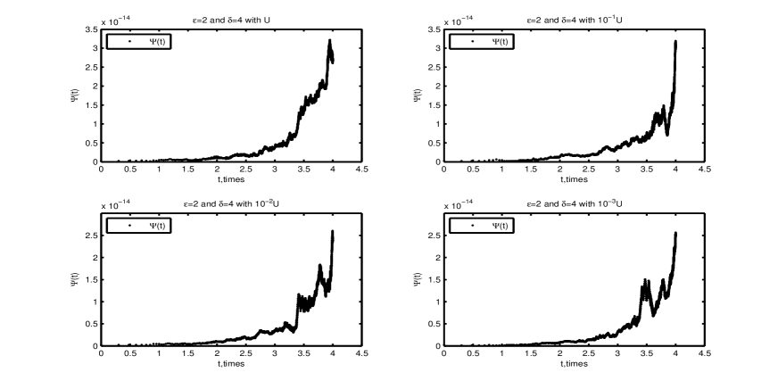
    Figure 1: Comparison of two solutions (Example 1)

    However, unperturbed system (6.3) is strongly stable. We remark that the rank $2$ perturbed system (4.3) of (6.3) is unstable for the matrix $U$ of rank $2$ and remains strongly stable for a matrix taken in $\{10^{-1}U,\;10^{-2}U,\;10^{-3}U\}$. Table 1 gives the different norms of projectors, the quantity $\delta_{S}$ and a convergence illustration of $S^{(n)}.$

    Table 1: Checking of the (strong) stability of (4.3) by the approachs defined in [3, 5] (Example 1)

    		U	$10^{-1}U$	$10^{-2}U$	$10^{-3}$	$U\equiv 0$
    $\|S^{(n)}\|$		$5.4202\times 10^{+33}$	7.9357	7.9838	7.9842	7.9842
    $\delta_{S}$		-	0.3645	0.3626	0.3625	0.3625
    $tr(\mathbb{P}_{0})$		$1$	$-2.6908\times 10^{-34}$	$5.3580\times 10^{-35}$	$1.0632\times 10^{-34}$	$1.9780\times 10^{-34}$
    $\|\mathbb{P}_{0}^{2}-\mathbb{P}_{0}\|_{2}$		$1.2741\times 10^{-16}$	$1.2611\times 10^{-34}$	$2.7797\times 10^{-34}$	$1.8430\times 10^{-34}$	$2.5227\times 10^{-34}$
    $tr(\mathbb{P}_{\infty})$		1	0	0	0	0
    $\|\mathbb{P}_{\infty}^{2}-\mathbb{P}_{\infty}\|_{2}$		$3.8592\times 10^{-16}$	$2.1197\times 10^{-35}$	$2.1197\times 10^{-35}$	$3.3161\times 10^{-35}$	$2.7261\times 10^{-35}$
    $tr(\mathbb{P}_{r})$		-	0	0	0	0
    $\|\mathbb{P}_{r}^{2}-\mathbb{P}_{r}\|_{2}$		-	0	0	0	0
    $tr(\mathbb{P}_{g})$		-	6	6	6	6
    $\|\mathbb{P}_{g}^{2}-\mathbb{P}_{g}\|_{2}$		-	$3.4285\times 10^{-19}$	$3.4285\times 10^{-19}$	$1.1102\times 10^{-16}$	0
    $\|\mathbb{P}_{r}+\mathbb{P}_{g}-I_{6}\|$		-	$3.4285\times 10^{-19}$	$3.4285\times 10^{-19}$	$1.1102\times 10^{-16}$	0

    Table 1 justifies the existence of a neighborhood in which any rank $2$ perturbation of the system remains strongly stable.

  • In Figure 3, we consider $U=V$ to perturb system (6.3). We can see that $\Psi(t)\leq 6\times 10^{-14}$ for all the figures. This shows that $\widetilde{X}(t)\equiv X_{1}(t),\;\forall\;t\in[0,\;\frac{2\pi}{\sqrt{7}}]$.

    

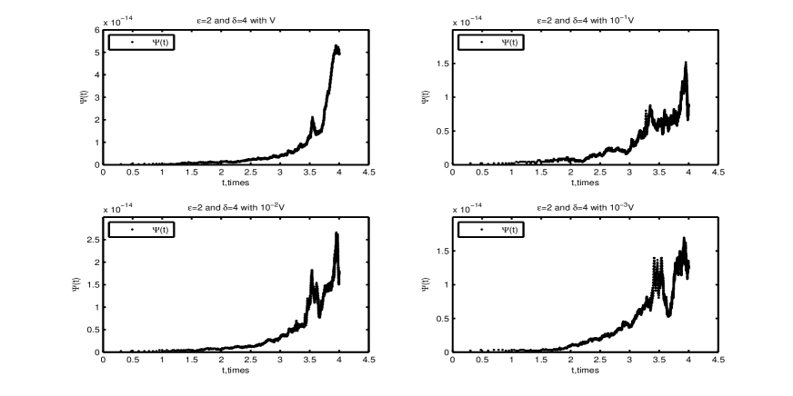
    Figure 2: Comparison of two solutions (Example 1)

  In this example, the unperturbed system is strongly stable for all $U$ taken in $\{10^{-1}V,10^{-2}V,10^{-3}V\}$ and not stable when $U=V$. This is illustrated in Table 2 which gives the norms of different projectors, the quantity $\delta$ and a convergence illustration of $S^{(n)}$.

  Table 2: Checking of the (strong) stability of (4.3) by the approachs defined in [3, 5] (Example 1)

  		U	$10^{-1}U$	$10^{-2}U$	$10^{-3}$	$U\equiv 0$
  $\|S^{(n)}\|$		$9.1853\times 10^{+33}$	7.9544	7.9839	7.9842	7.9842
  $\delta_{S}$		-	0.3645	0.3626	0.3625	0.3625
  $tr(\mathbb{P}_{0})$		$1$	$2.4361\times 10^{-35}$	$1.7323\times 10^{-35}$	$8.9556\times 10^{-35}$	$1.9780\times 10^{-34}$
  $\|\mathbb{P}_{0}^{2}-\mathbb{P}_{0}\|_{2}$		$1.3362\times 10^{-16}$	$2.3274\times 10^{-34}$	$1.4722\times 10^{-34}$	$1.2520\times 10^{-34}$	$2.5227\times 10^{-34}$
  $tr(\mathbb{P}_{\infty})$		1	0	0	0	0
  $\|\mathbb{P}_{\infty}^{2}-\mathbb{P}_{\infty}\|_{2}$		$3.6937\times 10^{-16}$	$2.6155\times 10^{-35}$	$8.4412\times 10^{-35}$	$3.4485\times 10^{-35}$	$2.7261\times 10^{-35}$
  $tr(\mathbb{P}_{r})$		-	0	0	0	0
  $\|\mathbb{P}_{r}^{2}-\mathbb{P}_{r}\|_{2}$		-	0	0	0	0
  $tr(\mathbb{P}_{g})$		-	6	6	6	6
  $\|\mathbb{P}_{g}^{2}-\mathbb{P}_{g}\|_{2}$		-	$5.4210\times 10^{-20}$	$2.5411\times 10^{-21}$	$1.1102\times 10^{-16}$	0
  $\|\mathbb{P}_{r}+\mathbb{P}_{g}-I_{6}\|$		-	$5.4210\times 10^{-20}$	$2.5411\times 10^{-21}$	$1.1102\times 10^{-16}$	0

  The second Table justifies the existence of a neighborhood in which any rank $3$ perturbation of the system remains strongly stable.

• for $\epsilon=15$ and $\delta=4$, we consider the random matrix $A={\small\left[\begin{array}[]{ccc}0.7482&0.8258&0.9619\\ 0.4505&0.5383&0.0046\\ 0.0838&0.9961&0.7749\\ 0.2290&0.0782&0.8173\\ 0.9133&0.4427&0.8687\\ 0.1524&0.1067&0.0844\\ \end{array}\right]}$. Using Algorithm 6.1 to matrix $A$, we obtain the matrix $V={\small\left[\begin{array}[]{ccc}-0.5773&-0.1332&0.4709\\ -0.3476&0.1520&0.1331\\ -0.0647&-0.9504&-0.2474\\ -0.1767&-0.1538&0.6077\\ -0.7047&0.1706&-0.5591\\ -0.1176&-0.0103&-.1320\\ \end{array}\right]}$ of rank $3$ whose columns span an isotropic subspace.

  • Let’s take $U=V(:,1:2)$. Figure 3 is obtained for values of any matrix of rank $2$ taken in $\{U,\;10^{-1}U,\;10^{-2}U,\;10^{-3}U\}.$ We remark that all the figures of Figure 3, verify $\Psi(t)\leq 1.4\times 10^{-12}$. This shows that $\widetilde{X}(t)\equiv X_{1}(t),\;\forall\,t\in[0,\;\frac{2\pi}{\sqrt{7}}].$

    

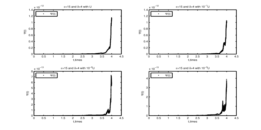
    Figure 3: Comparison of two solutions.

    In this example, the unperturbed system is unstable, and the rank $2$ perturbation systems remain unstable for any matrix of rank $2$ taken in $\{U,\;10^{-1}U,\;10^{-2}U,\;10^{-3}U\}$. This is illustrated in following Table 3

    Table 3: Checking of the (strong) stability of (4.3) by the dichotomy approach (Example 1)

    		U	$10^{-1}U$	$10^{-2}U$	$10^{-3}$	$U\equiv 0$
    $\|S^{(n)}\|$		$2.1415\times 10^{+48}$	$7.8057\times 10^{+32}$	$1.8698\times 10^{+35}$	$1.9709\times 10^{+35}$	$7.7999\times 10^{+41}$
    $\delta_{S}$		0	0	0	0	0
    $tr(\mathbb{P}_{0})$		2	2	2	2	2
    $\|\mathbb{P}_{0}^{2}-\mathbb{P}_{0}\|_{2}$		$7.1061\times 10^{-16}$	$3.7032\times 10^{-15}$	$9.4574\times 10^{-16}$	$2.6236\times 10^{-15}$	$3.7549\times 10^{-15}$
    $tr(\mathbb{P}_{\infty})$		2	2	2	2	2
    $\|\mathbb{P}_{\infty}^{2}-\mathbb{P}_{\infty}\|_{2}$		$1.1448\times 10^{-15}$	$7.4439\times 10^{-15}$	$4.0245\times 10^{-15}$	$2.5933\times 10^{-15}$	$3.8816\times 10^{-15}$

    Thus there doesn’t exist of a neighborhood of the unperturbed system in which any rank $2$ perturbation of the system is stable.

  • Taking $U=V$, Figure 4 shows that $\widetilde{X}(t)\equiv X_{1}(t),\;\forall\,t\in[0,\;\frac{2\pi}{\sqrt{7}}]$ for any matrix $U$ of rank $3$ taken in $\{U,\;10^{-1}U,\;10^{-2}U,\;10^{-3}U\}.$ In the first two subfigures of Figure 3, we see that $\Psi(t)\leq 1.4\times 10^{-12}$, while in the other subfigures, we note that $\Psi(t)\leq 8\times 10^{-13}.$

    

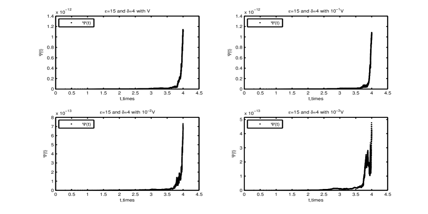
    Figure 4: Comparison of two solutions.

    However Table 4 shows that the perturbed system is not stable for any matrix taken in $\{U,10^{-1}U,10^{-2}U,10^{-2}U,O_{6}\}$.

    Table 4: Checking of the (strong) stability of (4.3) by the dichotomy approach (Example 1)

    		U	$10^{-1}U$	$10^{-2}U$	$10^{-3}$	$U\equiv 0$
    $\|S^{(n)}\|$		$1.3786\times 10^{+53}$	$5.7183\times 10^{+30}$	$1.7903\times 10^{+35}$	$1.9701\times 10^{+35}$	$1.9720\times 10^{+35}$
    $\delta_{S}$		0	0	0	0	0
    $tr(\mathbb{P}_{0})$		2	2	2	2	2
    $\|\mathbb{P}_{0}^{2}-\mathbb{P}_{0}\|_{2}$		$4.3586\times 10^{-16}$	$9.1634\times 10^{-16}$	$9.5301\times 10^{-16}$	$2.0073\times 10^{-156}$	$2.1088\times 10^{-15}$
    $tr(\mathbb{P}_{\infty})$		2	2	2	2	2
    $\|\mathbb{P}_{\infty}^{2}-\mathbb{P}_{\infty}\|_{2}$		$3.8829\times 10^{-16}$	$3.8684\times 10^{-15}$	$4.5557\times 10^{-15}$	$2.0032\times 10^{-15}$	$6.0387\times 10^{-15}$

Example 6.2

Consider the following differential system:

$$\left\{\begin{array}[]{lll}\dfrac{d^{2}\beta_{1}}{dt^{2}}+\left(4+a\cos(7t)\right)\beta_{1}+b\beta_{3}cos(14t)=0\\ \\ \dfrac{d^{2}\beta_{2}}{dt^{2}}+\left(a+b\sin(14t)\right)\beta_{2}+a\beta_{3}\sin(35t)=0\\ \\ \dfrac{d^{2}\beta_{3}}{dt^{2}}+3\beta_{3}+b\beta_{1}\cos(14t)+a\beta_{2}\sin(35t)=0\end{array}\right.,$$ (6.4)

where $a\in\mathbb{R}$ and $b\in\mathbb{R}^{\star}$ are real parameters. Let

$$\beta=\left(\begin{array}[]{c}\beta_{1}\\ \beta_{2}\\ \beta_{3}\par\end{array}\right)\quad x=\left(\begin{array}[]{c}\beta\\ \dfrac{d\beta}{dt}\end{array}\right).$$

System (6.4) can be written as a Hamiltonian of the form (1.2) with $T=\dfrac{2\pi}{7}$ and

$$P(t)=\left(\begin{array}[]{ccc}4+a\cos(7t)&0&b\cos(14t)\\ 0&a+b\sin(14t)&a\sin(35t)\\ b\cos(14t)&a\sin(35t)&3\end{array}\right)\quad\text{and}\quad H(t)=\left(\begin{array}[]{ccc}P(t)&0_{3}\\ 0_{3}&I_{3}\end{array}\right).$$

We show that the rank $k=2,3$ perturbation of the fundamental solution of (1.2) is the solution of its rank $k=2,3$ perturbation system. Consider

$$\Psi(t)=\|\widetilde{X}(t)-X_{1}(t)\|,\,\forall\,t\in[0,\;\frac{2\pi}{7}]$$

where $X_{1}(t)=(I+UU^{T}J)X(t)$ and $\widetilde{X}(t))_{t\in[0,\,\frac{2\pi}{7}]}$ is the solution of the rank $k=2,3$ perturbation Hamiltonian system (4.3) of (1.2). the following figures represent the norm of the difference between $\widetilde{X}_{1}(t)$ and $\widetilde{X}(t)$.

• for $a=2$ and $b=2,$ consider the random matrix $A=\left[\begin{array}[]{ccc}0.5377&-0.4336&0.7254\\ 1.8339&0.3426&-0.0631\\ -2.2588&3.5784&0.7147\\ 0.8622&2.7694&-0.2050\\ 0.3188&-1.3499&-0.1241\\ -1.3077&3.0349&1.4897\\ \end{array}\right]$. Applying Algorithm 6.1 to matrix $A$, we get the following matrix

  $$V=\left[\begin{array}[]{ccc}-0.1599&0.0405&0.5357\\ -0.5453&-0.3844&0.2439\\ 0.6717&-0.4143&0.1441\\ -0.2564&-0.7645&-0.1887\\ -0.0948&0.1272&0.6857\\ 0.3889&-0.2798&0.3563\end{array}\right]$$

  of rank 3 whose columns generate an isotropic subspace.

  • Considering the matrix $U=V(:,1:2)$, we get Figure 5 perturbing system (1.2) by matrices taken in $\{U,\;10^{-1}U,\;\;10^{-2}U,\;\;10^{-3}U\}$.

    In Figure 5, we note that all the figures verify $\Psi(t)\leq 2.5\times 10^{-14}$. This shows that $\widetilde{X}(t)\equiv X_{1}(t),\;\forall\;t\in[0,\;\frac{2\pi}{7}].$

    

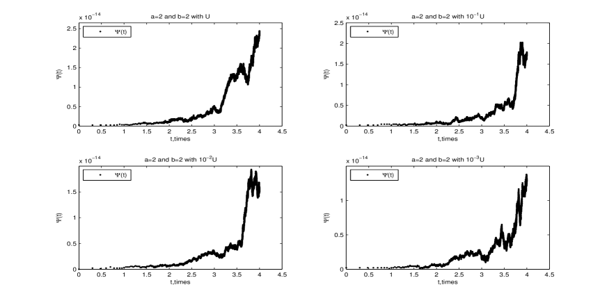
    Figure 5: Comparison of two solutions (Example 2)

    In this first example, the unperturbed system is strongly stable and the rank $2$ perturbation of the system is also strongly stable for any matrix of rank $2$ belonging to $\{10^{-1}U,\;\;10^{-2}U,\;\;10^{-3}U\}$ and is unstable for any matrix of rank $2$ with $U$. This discussion is summaries in Table $5$

    Table 5: Checking of the (strong) stability of (4.3) by the approachs defined in [3, 5] (Example 2)

    		$U$	$10^{-1}U$	$10^{-2}U$	$10^{-3}U$	$U\equiv 0$
    $\|S^{(n)}\|,\;(n=30)$		$7.8892$	$2.1128$	$2.1115$	$2.1115$	$2.1115$
    $\delta_{S}$		$0.4628$	$0.2574$	$0.2528$	$0.2528$	$0.2528$
    $tr(\mathbb{P}_{0})$		$-4.2126\times 10^{-17}$	$-1.9678\times 10^{-16}$	$1.3498\times 10^{-16}$	$-2.2171\times 10^{-16}$	$-4.2126\times 10^{-17}$
    $\|\mathbb{P}_{0}^{2}-\mathbb{P}_{0}\|_{2}$		$1.3434\times 10^{-16}$	$1.1411\times 10^{-16}$	$1.1709\times 10^{-16}$	$1.4804\times 10^{-16}$	$1.3434\times 10^{-16}$
    $tr(\mathbb{P}_{\infty})$		$-3.6385\times 10^{-17}$	$-1.0876\times 10^{-17}$	$-9.4959\times 10^{-17}$	$-2.2708\times 10^{-16}$	$-3.6385\times 10^{-17}$
    $\|\mathbb{P}_{\infty}^{2}-\mathbb{P}_{\infty}\|_{2}$		$1.4218\times 10^{-16}$	$1.4991\times 10^{-16}$	$1.0851\times 10^{-16}$	$1.7867\times 10^{-16}$	$1.4218\times 10^{-16}$
    $tr(\mathbb{P}_{r})$		$6$	$6$	$6$	$6$	$6$
    $\|\mathbb{P}_{r}^{2}-\mathbb{P}_{r}\|_{2}$		$0$	$0$	$0$	$0$	$0$
    $tr(\mathbb{P}_{g})$		$0$	$0$	$0$	$0$	$0$
    $\|\mathbb{P}_{g}^{2}-\mathbb{P}_{g}\|_{2}$		$0$	$0$	$0$	$0$	$0$
    $\|\mathbb{P}_{r}+\mathbb{P}_{g}-I_{6}\|_{2}$		$0$	$0$	$0$	$0$	$0$

    This justifies the existence of a neighborhood of the unperturbed system in which any random rank $2$ perturbation of the system remains strongly stable.

  • Let’s take $U=V$ ; Figure 6 shows that $\Psi(t)<3.5\times 10^{-14},\,\forall\,t\in[0,\;\frac{2\pi}{7}]$ for all the figures. This shows that $\widetilde{X}(t)\equiv X_{1}(t).$

    

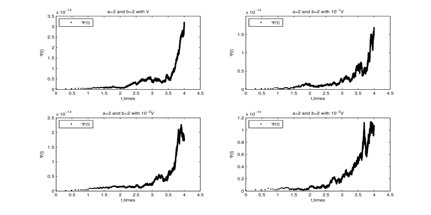
    Figure 6: Comparison of two solutions (Example 2)

    In this case, the unperturbed system (1.2) is strongly stable for any random matrix $U$ of rank $3$ belonging to $\{V,\;10^{-1}V,\;10^{-2}V,\,10^{-3}V\}$. This is illustrated in Table 6

    Table 6: Checking of the (strong) stability of (4.3) by the approachs defined in [3, 5] (Example 2)

    		$V$	$10^{-1}V$	$10^{-2}V$	$10^{-3}V$	$V\equiv 0$
    $\|S^{(n)}\|,\;(n=30)$		$11.8852$	$2.1209$	$2.1116$	$2.1115$	$2.1115$
    $\delta_{S}$		$0.3599$	$0.2532$	$0.2528$	$0.2528$	$0.2528$
    $tr(\mathbb{P}_{0})$		$-2.0382\times 10^{-16}$	$1.2364\times 10^{-16}$	$1.0578\times 10^{-18}$	$-9.0143\times 10^{-17}$	$-4.2126\times 10^{-17}$
    $\|\mathbb{P}_{0}^{2}-\mathbb{P}_{0}\|_{2}$		$1.1186\times 10^{-16}$	$1.7572\times 10^{-16}$	$5.8457\times 10^{-17}$	$8.4476\times 10^{-17}$	$1.3434\times 10^{-16}$
    $tr(\mathbb{P}_{\infty})$		$-2.2819\times 10^{-16}$	$-1.0701\times 10^{-17}$	$-6.8127\times 10^{-19}$	$-1.0956\times 10^{-17}$	$-3.6385\times 10^{-17}$
    $\|\mathbb{P}_{\infty}^{2}-\mathbb{P}_{\infty}\|_{2}$		$1.1307\times 10^{-16}$	$2.5771\times 10^{-16}$	$6.3190\times 10^{-17}$	$1.1784\times 10^{-16}$	$1.4218\times 10^{-16}$
    $tr(\mathbb{P}_{r})$		$6$	$6$	$6$	$6$	$6$
    $\|\mathbb{P}_{r}^{2}-\mathbb{P}_{r}\|_{2}$		$0$	$0$	$0$	$0$	$0$
    $tr(\mathbb{P}_{g})$		$0$	$0$	$0$	$0$	$0$
    $\|\mathbb{P}_{g}^{2}-\mathbb{P}_{g}\|_{2}$		$0$	$0$	$0$	$0$	$0$
    $\|\mathbb{P}_{r}+\mathbb{P}_{g}-I_{6}\|_{2}$		$0$	$0$	$0$	$0$	$0$

    This justifies the existence of a neighborhood of the unperturbed system in which any random rank $3$ perturbation of the system remains strongly stable.

• For $a=18.95$ and $b=2,$ consider the random matrix

  $$A=\left[\begin{array}[]{ccc}1.4090&0.4889&0.8884\\ 1.4172&1.0347&-1.1471\\ 0.6715&0.7269&-1.0689\\ -1.2075&-0.3034&-0.8095\\ 0.7172&0.2939&-2.9443\\ 1.6302&-0.7873&1.4384\end{array}\right].$$

  Applying the algorithm 6.1 to the matrix $A$, we have the following random matrix

  $$V=\left[\begin{array}[]{ccc}-0.4677&-0.3232&0.6729\\ -0.4704&-0.4311&-0.3311\\ -0.2229&-0.1819&0.2867\\ 0.4008&-0.1814&0.1744\\ -0.2381&-0.3203&-0.5692\\ -0.5412&0.7356&-0.0323\end{array}\right]$$

  of rank $3$ whose columns generate an isotropic subspace.

  • Let’s take $U=V(:,1:2)$. The following Figure shows that $\widetilde{X}(t)\equiv X_{1}(t),\;\,\forall\;t\in[0,\;\frac{2\pi}{7}]$, for any matrix of rank $2$ belonging to $\{U,\;10^{-1}U,\;10^{-2}U,\;10^{-3}U\}.$ Thus in Figure 7, we can observe that $\Psi(t)\leq 1\times 10^{-13},\,\forall\,t\in[0,\;\frac{2\pi}{7}]$ for all figures.

    

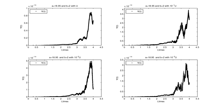
    Figure 7: Comparison of two solutions (Example 2)

    In this case, the unperturbed system is unstable and its rank $2$ perturbation systems remain unstable for any matrix of rank $2$ taken in $\{U,\,10^{-1}U,\;10^{-2}U,\;10^{-3}U\}$. This is illustrated in Table 7

    Table 7: Checking of the (strong) stability of (4.3) by the approachs defined in [3, 5] (Example 2)

    		$U$	$10^{-1}U$	$10^{-2}U$	$10^{-3}U$	$U\equiv 0$
    $\|S^{(n)}\|,\;(n=30)$		$4.9239\times 10^{+57}$	$5.7014\times 10^{+45}$	$5.2235\times 10^{+45}$	$5.2189\times 10^{+45}$	$5.2189\times 10^{+45}$
    $tr(\mathbb{P}_{0})$		$2$	$1$	$1$	$1$	$1$
    $\|\mathbb{P}_{0}^{2}-\mathbb{P}_{0}\|_{2}$		$7.3293\times 10^{-16}$	$3.0130\times 10^{-16}$	$1.8699\times 10^{-16}$	$1.8367\times 10^{-16}$	$7.4397\times 10^{-17}$
    $tr(\mathbb{P}_{\infty})$		$2$	$1$	$1$	$1$	$1$
    $\|\mathbb{P}_{\infty}^{2}-\mathbb{P}_{\infty}\|_{2}$		$1.6104\times 10^{-15}$	$2.0658\times 10^{-16}$	$2.2422\times 10^{-16}$	$1.0577\times 10^{-15}$	$1.1106\times 10^{-15}$

    This justifies the existence of a neighborhood of the unperturbed system in which any rank $2$ perturbation of the system remains unstable.

  • In this latter example, we consider $U=V$ to perturb system (1.2). Figure 8 is obtained for value of any random matrix $U$ of rank $3$ taken in $\{U,\,10^{-1}U,\,10^{-2}U,\,10^{-3}U\}$. We can see that $\Psi(t)\leq 5.25\times 10^{-14},\,\forall\,t\in[0,\;\frac{2\pi}{7}]$ for all figures. Hence, we have $\widetilde{X}(t)\equiv X_{1}(t),\;\,\forall\;t\in[0,\;\frac{2\pi}{7}]$.

    

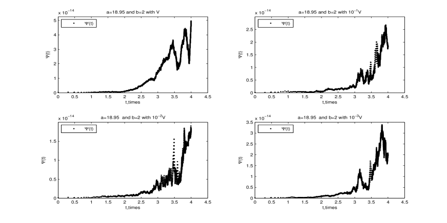
    Figure 8: Comparison of two solutions (Example 2)

    However the following Table 8 shows that the perturbed system is not stable for any random matrix $U$ of rank $3$ taken in $\{U,\;10^{-1}U,\;10^{-2}U,\;10^{-3}U,\,O_{6,3}\}$.

    Table 8: Checking of the (strong) stability of (4.3) by the approachs defined in [3, 5] (Example 2)

    		$U$	$10^{-1}U$	$10^{-2}U$	$10^{-3}U$	$U\equiv 0$
    $\|S^{(n)}\|,\;(n=30)$		$1.6182\times 10^{+55}$	$7.3921\times 10^{+45}$	$5.2372\times 10^{+45}$	$5.2191\times 10^{+45}$	$5.2189\times 10^{+45}$
    $tr(\mathbb{P}_{0})$		$2$	$1$	$1$	$1$	$1$
    $\|\mathbb{P}_{0}^{2}-\mathbb{P}_{0}\|_{2}$		$2.0170\times 10^{-16}$	$1.3412\times 10^{-16}$	$2.9536\times 10^{-16}$	$2.0371\times 10^{-16}$	$7.4397\times 10^{-17}$
    $tr(\mathbb{P}_{\infty})$		$2$	$1$	$1$	$1$	$1$
    $\|\mathbb{P}_{\infty}^{2}-\mathbb{P}_{\infty}\|_{2}$		$8.5346\times 10^{-16}$	$5.0453\times 10^{-16}$	$4.8715\times 10^{-16}$	$1.0011\times 10^{-15}$	$1.1106\times 10^{-15}$

7 Concluding remarks

In this research work, after defining a rank $k$ perturbation theory of a Hamiltonian system with periodic coefficients with $k\geq 2$, we showed that the solution of its rank $k$ perturbation is the same as the rank $k$ perturbation of the solution of unperturbed system. Then we analyzed Jordan canonical form of the solution of the unperturbed system when it is subjected to a rank $k$ perturbation. This analysis is a generalization of that made by M. Dosso, et al. in [2] in the case of a rank one pertubation of Hamiltonian system with periodic coefficients. Finally we proposed numerical examples which confirm this theory. However, these examples use an algorithm that randomly constructs an isotropic subspace basis. From these numerical examples we notice that when a system is strongly stable (respectively unstable), there exists a neighborhood in which any rank $k$ perturbation of the system in this neighborhood remains strongly stable (respectively unstable)

In future work, we will compare the zone of stability (strong) of the Hamiltonian systems with periodic coefficients and their rank $k\geq 1$ perturbations. Then it would be boring to find a link between any random perturbation and rank $k\geq 1$ perturbation of Hamiltonian system with periodic coefficients.

References

- [1] C. Brezinski, Computational Aspects of Linear Control, Kluwer Academic Publishers, 2002.
- [2] M.Dosso, T.G.Y. Arouna., and J.C.Koua. Brou, On rank one perturbations of Hamiltonian system with periodic coefficients. Wseas Translations on Mathematics. Volume 15, 2016, Pages 502-510.
- [3] M. Dosso and M. Sadkane. On the strong stability of symplectic matrices. Numerical Linear Algebra with Applications 20(2) (2013), 234-249.
- [4] M.Dosso and N. Coulibaly, Symplectic matrices and strong stability of Hamiltonian systems with periodic coefficients. Journal of Mathematical Sciences : Advances and Applications. Vol. 28(2014), pp 15-38.
- [5] M. Dosso, N. Coulibaly and L. Samassi, Strong stability of symplectic matrices using a spectral dichotomy method, Far East Journal Applied Mathematics. Vol. 79, No 2, 2013, pp 73-110.
- [6] G. Freiling, V. Mehrmann, and H. Xu. Existence, uniqueness and parametrization of Lagrangian invariant subspaces. SIAM J. Matrix Anal. Appl., 23:10451069, 2002.
- [7] Godunov SK, Verification of boundedness for the powers of symplectic matrices with the help of averaging. Siber. Math. J. 1992 ; 33 : 939-949.
- [8] S.K. Godunov, Stability of iterations of symplectic transformations, Siberian Math. J. 30, 54-63 (1989).
- [9] S.K. Godunov, M. Sadkane, Numerical determination of a canonical form of a symplectic matrix, Siberian Math. J. 42, 629-647 (2001)
- [10] S.K. Godunov, M. Sadkane, Spectral analysis of symplectic matrices with application to the theory of parametric resonance, SIAM J. Matrix Anal. Appl. 28, 1083-1096 (2006)
- [11] I. Gohberg, P. Lancaster, and L. Rodman. Indefinite Linear Algebra and Applications. Birkhäuser, Basel, 2005.
- [12] B. Hassibi, A. H. Sayed, T. Kailath, Indefinite-Quadratic Estimation and Control, SIAM, Philadelphia, PA, 1999.
- [13] D. Kressner, Perturbation bounds for isotropic invariant subspaces of skew-Hamiltonian matrices. SIAM J. Matrix Analysis Applications 26(4): 947-961, 2005.
- [14] D. Kressner, Numerical Methods for General and Structured Eigenvalue Problems. Lecture Notes in Computational Science and Engineering 46, Springer 2005. ISBN 978-3-540-24546-9, pp. I-XIV, 1-264.
- [15] P. Lancaster and L. Rodman. The Algebraic Riccati Equation. Oxford University Press, Oxford, 1995.
- [16] C. Mehl, V. Mehrmann, A. C. M. Ran and L. Rodman. Eigenvalues Perturbation theory of structured matrices under generic structured rank one perturbations ; Symplectic, othogonal and unitary matrices. BIT, 54(2014), 219-255.
- [17] C. Mehl, V. Mehrmann, A. C. M. Ran and L. Rodman. Perturbation analysis of Lagrangian invariant subspaces of symplectic matrices. Linear and Multilinear Algebra, 57:141-184, 2009.
- [18] Y. Saad, Numerical methods for large eugenvalue problems. SIAM, 2nd ed., 2011.
- [19] D. S. Watkins, The matrix eigenvalue problem. GR and Krylov Subspace Methods ,SIAM, Philadelphia, 2007.
- [20] V.A. Yakubovich, V.M. Starzhinskii, Linear differential equations with periodic coefficients, Vol. 1 & 2., Wiley, New York (1975)
- [21] YAN Qing-you. The properties of a kind og random symplectic matrices. Applied mathematics and Mechanics. Vol 23, No 5, May 2002.