Steering the distribution of agents
in mean-field and cooperative games

Abstract

The purpose of this work is to pose and solve the problem to guide a collection of weakly interacting dynamical systems (agents, particles, etc.) to a specified terminal distribution. The framework is that of mean-field and of cooperative games. A terminal cost is used to accomplish the task; we establish that the map between terminal costs and terminal probability distributions is onto. Our approach relies on and extends the theory of optimal mass transport and its generalizations.

Keywords: Mean-field games, linear stochastic systems, weakly interacting particle system, McKean-Vlasov dynamics, optimal control.

I Introduction

Mean-field game (MFG) theory is the study of noncooperative games involving a large number of agents. The basic model requires agents to abide by identical dynamics and seek to minimize an individual cost function that is also the same for all. As the number of agents increases to infinity, the empirical distribution of their states becomes indifferent to the strategy of any single agent and yet it couples their individual responses. Thus, the aggregate response of the agents (mean field) drives individual responses while the action of individual agents is insignificant. On the flip side, cooperative games refer to the situation where agents seek to jointly optimize a common performance index. Either way, the desire to minimize cost, individually or collectively, drives the empirical distribution of agents in suitable ways. The purpose of this work to study for both, MFG and cooperative games, the control problem to steer the collective response of agents over a finite window of time between two specified end-point marginal distributions by suitable choice of cost (i.e., incentives) in non-cooperative games and centralized control with cooperative agents, and also the problem to ensure a desired stationary distribution under similar conditions. This viewpoint is influenced by optimal mass transport (OMT) theory that deals with the flow of time-marginal densities for a collective (agents, particles, resources) and corresponding control and modeling problems.

The study of MFG’s was introduced into the engineering literature by Huang, Malhamé and Caines [1] and, independently, by Lasry and Lions [2]. Earlier, in the economics literature, similar models were considered by Jovanovic and Rosental [3]. The importance of the subject stems from the wide range of applications that include modeling and control of multi-agent dynamical systems, stock market dynamics, crowd dynamics, power systems and more; see [1, 2, 4, 5], and also see [6, 7, 8, 9] in the special case of linear dynamics and quadratic cost. On the other hand, OMT originates in the work of Monge [10] and aims directly at relating/transporting distributions under minimum cost. Kantorovich [11] introduced linear programming and duality theory for solving OMT resource allocation problems and, in recent years, a fast developing phase was spurred by a wide range of applications of OMT to probability theory, economics, weather modeling, biology and mathematical physics [12, 13, 14, 15, 16, 17, 18, 19]. The connection between dynamic OMT [20] and stochastic control has been explored in our work, e.g. [21, 22], where the focus has been on regulating stochastic uncertainty of diffusion processes and of stochastically driven dynamical systems by suitable control action. These stochastic control problems, in turn, relate to a classical maximum entropy problem on path space known as the Schrödinger bridge problem, see e.g., [23, 24, 25, 26, 27, 28].

The goal of the present work is to study density steering problems in an MFG framework or, equivalently, explore the role of interaction potential and decentralized strategies when steering an initial distribution to a terminal one. In particular, we are interested on how to design an added terminal cost so as to provide incentives for agents, under a Nash equilibrium strategy, to move collectively as specified. To this end, we establish that the map between terminal costs and terminal probability distributions is onto. Thereby, we develop an MFG-based synthesis framework for OMT-type stochastic control problems with or without stochastic excitation.

The paper evolves along the following lines. First, we discuss the motivation and problem formulation in Section II. The solution is provided in Section III. In Section IV we study similar problems with less or no disturbance. Section V is dedicated to the special case with Gaussian marginal distributions. Similar problems in the stationary setting are investigated in Section VI. In Section VII, we developed the cooperative game counterpart of the density steering problem. This follows by a simple academic example in Section VIII and a brief concluding remark in Section IX.

II Problem formulation

We herein investigate the collective dynamical response of a group of agents (also thought of as particles, players, and so on) that interact weakly with each other. The terminology “weakly” refers to the agents being statistically indistinguishable (anonymous) and affecting each other’s response only through their empirical distribution [29]. Thus, we consider such a system of $N$ agents with dynamics specified by

$$dx_{i}(t) = Ax_{i}(t)dt+\frac{1}{N-1}\sum_{j\neq i}{\bar{A}}x_{j}(t)dt+Bu_{i}(t)dt+Bdw_{i}(t),$$

$$~{}~{}x_{i}(0)=x_{0}^{i},~{}~{}i=1,\ldots,N.$$

Here, $x_{i},u_{i},w_{i}$ represent the state, control input, white noise disturbance, respectively, for the $i$th agent, and the model parameters are the same for all. We further assume that their initial conditions $x_{0}^{1},x_{0}^{2},\ldots,x_{0}^{N}$ are all independent with the same probability density $\rho_{0}$. The $i$th agent interacts with the rest through the averaged position. The matrices $A,\bar{A}\in{\mathbb{R}}^{n\times n},B\in{\mathbb{R}}^{n\times m}$ are continuous functions of time; for notational simplicity we often use e.g., $A$ instead of $A(t)$. It is assumed that the pair is controllable in the sense that the reachability Gramian

$$M(t,s)=\int_{s}^{t}\Phi(t,\tau)B(\tau)B(\tau)^{\prime}\Phi(t,\tau)^{\prime}d\tau$$

is invertible for all $s<t$. Here, $\Phi(\cdot,\cdot)$ denotes the state transition matrix that is defined via

$$\frac{\partial\Phi(t,s)}{\partial t}=A\Phi(t,s),~{}~{}\Phi(s,s)=I.$$

Clearly, in case when $A$ is time-invariant, $\Phi(t,s)=e^{A(t-s)}$.

In MFG [1], each agent searches for an optimal control strategy to minimize its own cost

$$J_{i}(u_{i})={\mathbb{E}}\left\{\int_{0}^{1}f(t,x_{i}(t),u_{i}(t),\mu^{N}(t))dt+g(x_{i}(1),\mu^{N}(1))\right\},$$ (2)

where

$$\mu^{N}(t)=\frac{1}{N}\sum_{i=1}^{N}\delta_{x_{i}(t)}$$ (3)

is the empirical distribution of the states of the $N$ agents at time $t$. Thus, this is a non-cooperative game and the cost of the $i$th agent is affected by the strategies of others only through the empirical distribution. An optimal control corresponds to a Nash equilibrium for the game. We follow the arguments in [5], and restrict ourselves to equilibria that correspond to symmetric Markovian control strategies (state feedback)

$$u_{i}(t)=\phi(t,x_{i}(t)),i=1,\ldots,N.$$ (4)

When $N$ is large, the empirical distribution $\mu^{N}$ is indifferent to small perturbations of control strategy of a single agent. This points to the following approach [5] to obtain an approximate Nash equilibrium: fix a family $(\mu(t))_{0\leq t\leq 1}$ of probability measures and solve the standard stochastic control problem

$$\phi^{\star}=\operatorname{argmin}_{\phi}{\mathbb{E}}\left\{\int_{0}^{1}f(t,x(t),\phi(t,x(t)),\mu(t))dt+g(x(1),\mu(1))\right\}$$ (5)

subject to the dynamics

$$dx(t)=Ax(t)dt+{\bar{A}}{\bar{x}_{\mu}}(t)dt+B\phi(t,x(t))dt+Bdw(t),~{}~{}x(0)=x_{0}~{}\mbox{a.s.}$$ (6)

where

$$\bar{x}_{\mu}:=\langle x,\mu(t)\rangle$$

denotes the mean of the distribution $\mu(t)$, and $x_{0}$ is a random vector with probability density $\rho_{0}$. Considering the choice $(\mu(t))_{0\leq t\leq 1}$ as a parameter, the remaining issue is to choose this distribution flow so that the actual distribution of the solution $x(t)$ of (6) with optimal control strategy

$$u^{\star}(t)=\phi^{\star}(t,x(t))$$ (7)

coincides with $\mu(t)$. The solution to the MFG problem involves establishing the existence and uniqueness of the solution to two coupled partial differential equations (PDEs) [5]. It has been shown that a Nash equilibrium point for this mean-field game exists under rather mild assumptions on the cost function [1, 2, 4, 5, 6, 7, 8, 9]. That is, there exists a family $(\mu(t))_{0\leq t\leq 1}$ such that the distribution flow of the solution $x(t)$ of (6) under optimal control strategy $\phi^{\star}$ coincides with this same $\mu$. In addition, this optimal control $\phi^{\star}$ is proven to be an $\varepsilon$-Nash equilibrium to the $N$-player-game for $N$ large [5, 30].

Departing from previous literature, this paper deals with the density steering problem of the $N$-player-game system. More specifically, we are interested in introducting a suitable cost incentive so that the system is driven to a specific distribution $\mu_{1}$ at time $t=1$ under (7). In fact, it turns out that under mild conditions, a quadratic running cost in both the control and state (i.e., group linear tracking as in the work of Huang, Malamé and Caines [1]), can be enhanced by a suitable terminal cost $g$ as follows

$$J_{i}(u_{i})={\mathbb{E}}\left\{\int_{0}^{1}\left(\frac{1}{2}\|u_{i}(t)\|^{2}+\frac{1}{2}\|x_{i}(t)-\bar{x}(t)\|_{Q}^{2}\right)dt+g(x_{i}(1),\mu^{N}(1))\right\}$$ (8)

so as to acomplish the task of steering the initial distribution to the desired terminal one. In other words, we show that the mapping between a choice of $g$ and the terminal distribution $\mu_{1}$ is onto. Formally, the problem we are interested in can be stated as follows.

Problem 1

Given $N$ agents governed by (II) with initial probability density $\rho_{0}$, find a terminal cost $g$ such that, in the Nash equilibrium with cost functional (8), the agents will reach a given terminal density $\rho_{1}$ at time $t=1$, in the limit as $N$ goes to $\infty$.

III General approach and solution

Without loss of generality and for simplicity of the exposition we only consider a running cost only in the control actuation (i.e., taking the matrix $Q$ in (8) to be zero). We begin by considering the optimal steering problem [31, 27, 28, 32] without terminal cost, i.e., for a fixed density flow $(\mu(t))_{0\leq t\leq 1}$, consider the control problem to minimize

$$J(u)={\mathbb{E}}\left\{\int_{0}^{1}\frac{1}{2}\|u(t)\|^{2}dt\right\}$$

subject to the dynamics

$$dx(t)=Ax(t)dt+{\bar{A}}{\bar{x}_{\mu}}(t)dt+Bu(t)dt+Bdw(t),~{}~{}x(0)=x_{0}\sim\rho_{0}~{}$$ (9)

and the constraint that $x(1)$ has probability density $\rho_{1}$. This problem can be (formally) posed as

$$\inf_{\rho,u}\quad\int_{0}^{1}\int_{{\mathbb{R}}^{n}}\frac{1}{2}\rho(t,x)\|u(t,x)\|^{2}dxdt,$$ (10a)

$$\frac{\partial\rho}{\partial t}+\nabla\cdot((Ax+{\bar{A}}{\bar{x}_{\mu}}+Bu)\rho)-\frac{1}{2}\operatorname{tr}(BB^{\prime}\nabla^{2}\rho)=0,$$ (10b)

$$\rho(0,\cdot)=\rho_{0},\quad\rho(1,\cdot)=\rho_{1}.$$ (10c)

Following a similar argument as in [22], we can establish the following sufficient condition for optimality.

Proposition 1

If there exists a function $\lambda$ such that $\rho^{\star},\lambda$ satisfy

$$\frac{\partial\lambda}{\partial t}+\nabla\lambda\cdot Ax+\nabla\lambda\cdot{\bar{A}}{\bar{x}_{\mu}}+\frac{1}{2}\operatorname{tr}(BB^{\prime}\nabla^{2}\lambda)+\frac{1}{2}\nabla\lambda\cdot BB^{\prime}\nabla\lambda=0,$$ (11a)

$$\frac{\partial\rho^{\star}}{\partial t}+\nabla\cdot((Ax+{\bar{A}}{\bar{x}_{\mu}}+BB^{\prime}\nabla\lambda)\rho^{\star})-\frac{1}{2}\operatorname{tr}(BB^{\prime}\nabla^{2}\rho^{\star})=0,$$ (11b)

and boundary conditions

$$\rho^{\star}(0,\cdot)=\rho_{0},\quad\rho^{\star}(1,\cdot)=\rho_{1},$$ (11c)

then $(\rho^{\star},u^{\star}=B^{\prime}\nabla\lambda)$ is a solution to (36).

Replacing $\mu$ in (11) by $\rho^{\star}$ we obtain the system of (nonlinear) PDE’s

$$\frac{\partial\lambda}{\partial t}+\nabla\lambda\cdot Ax+\nabla\lambda\cdot{\bar{A}}\bar{x}_{\rho^{\star}}+\frac{1}{2}\operatorname{tr}(BB^{\prime}\nabla^{2}\lambda)+\frac{1}{2}\nabla\lambda\cdot BB^{\prime}\nabla\lambda=0,$$ (12a)

$$\frac{\partial\rho^{\star}}{\partial t}+\nabla\cdot((Ax+{\bar{A}}\bar{x}_{\rho^{\star}}+BB^{\prime}\nabla\lambda)\rho^{\star})-\frac{1}{2}\operatorname{tr}(BB^{\prime}\nabla^{2}\rho^{\star})=0,$$ (12b)

$$\rho^{\star}(0,\cdot)=\rho_{0},\quad\rho^{\star}(1,\cdot)=\rho_{1}.$$ (12c)

We will show below that, under mild assumptions, (12) has a solution. In fact, we will construct such a solution relying on standard Schrödinger bridge theory [21, 22].

Remark 2

Note that the coupled PDEs (12a-12b) are the same as the PDEs that arise in classic MFG problems corresponding to (II) and (8). However, the usual boundary conditions

$$\rho^{\star}(0,\cdot)=\rho_{0},\quad\lambda(1,x)=-g(x,\rho^{\star}(1,\cdot)),$$

are now different and given by (12c). Evidently, the Lagrange multiplier $-\lambda$ is the value (cost-to-go) function of the associated optimal control problem.

To solve (12), we first consider the Schrödinger bridge problem with prior dynamics

$$dx(t)=Ax(t)dt+Bdw(t).$$ (13)

Let

$$\hat{\rho}_{0}(x)=\rho_{0}(x+\bar{x}_{\rho_{0}})$$

and

$$\hat{\rho}_{1}(x)=\rho_{1}(x+\bar{x}_{\rho_{1}}),$$

then

$$\langle x,\hat{\rho}_{0}\rangle=0,~{}~{}\langle x,\hat{\rho}_{1}\rangle=0.$$

The Schrödinger bridge with prior dynamics (13) and marginal distributions $\hat{\rho}_{0}$ and $\hat{\rho}_{1}$ is [21, 22]

$$dx(t)=Ax(t)dt+BB^{\prime}\nabla\hat{\lambda}(t,x(t))dt+Bdw(t),$$ (14)

where $\hat{\lambda}$ satisfies

$$\frac{\partial\hat{\lambda}}{\partial t}+\nabla\hat{\lambda}\cdot Ax+\frac{1}{2}\operatorname{tr}(BB^{\prime}\nabla^{2}\hat{\lambda})+\frac{1}{2}\nabla\hat{\lambda}\cdot BB^{\prime}\nabla\hat{\lambda}=0,$$ (15)

or, equivalently, $\varphi=\exp(\hat{\lambda})$ satisfies

$$\frac{\partial\varphi}{\partial t}+\nabla\varphi\cdot Ax+\frac{1}{2}\operatorname{tr}(BB^{\prime}\nabla^{2}\varphi)=0.$$

The boundary condition $\hat{\lambda}(1,\cdot)$ for $\hat{\lambda}$ is chosen in a way so that the resulting density flow $\hat{\rho}(t,x)$ of (14), which is

$$\frac{\partial\hat{\rho}}{\partial t}+\nabla\cdot((Ax+BB^{\prime}\nabla\hat{\lambda})\hat{\rho})-\frac{1}{2}\operatorname{tr}(BB^{\prime}\nabla^{2}\hat{\rho})=0,$$

matches the marginal distributions $\hat{\rho}_{0}$ and $\hat{\rho}_{1}$. The pair $(\hat{\lambda},\hat{\rho})$ satisfies that

$$\langle\nabla\hat{\lambda}(t,\cdot),\hat{\rho}(t,\cdot)\rangle=0$$ (16)

and therefore

$$\langle x,\hat{\rho}(t,\cdot)\rangle=0$$ (17)

for all $0\leq t\leq 1$. The intuition is that if the expectation of the control, i.e., $\langle\nabla\hat{\lambda}(t,\cdot),\hat{\rho}(t,\cdot)\rangle$, is not constantly $0$, then one can always shift the control by its mean to achieve a smaller cost. Now let

$$m(t)=\Phi(1,t)^{\prime}\bar{M}_{10}^{-1}(\bar{x}_{\rho_{1}}-\bar{\Phi}_{10}\bar{x}{\rho_{0}}),$$

$y(t)$ the solution to

$$\dot{y}(t)=(A+{\bar{A}})y(t)+BB^{\prime}m(t),~{}~{}y(0)=\bar{x}_{\rho_{0}},$$

and

$$\gamma(t)=-\int_{0}^{t}({\bar{A}}y(s)\cdot m(s)+\frac{1}{2}m(s)\cdot BB^{\prime}m(s))ds.$$

Here $\bar{\Phi}_{10}:=\bar{\Phi}(1,0)$ with $\bar{\Phi}$ being the state transition matrices for the pair $(A+{\bar{A}},B)$ and the “coupled” Gramian

$$\bar{M}_{10}=\int_{0}^{1}\bar{\Phi}(1,\tau)BB^{\prime}\Phi(1,\tau)^{\prime}d\tau$$

is assumed to be invertible. Note that $y(1)=\bar{x}_{\rho_{1}}$.

With these ingredients, we construct a solution to (12) as follows. Define $(\lambda,\rho^{\star})$ by

$$\lambda(t,x)=\hat{\lambda}(t,x-y(t))+m(t)\cdot x+\gamma(t),$$ (18a)

and

$$\rho^{\star}(t,x)=\hat{\rho}(t,x-y(t)).$$ (18b)

In so doing, $(\lambda,\rho^{\star})$ is a solution of (12). On one hand, substituting (18) into (12b), in view of (17), we obtain

$$\frac{\partial\rho^{\star}}{\partial t}+\nabla\cdot((Ax+{\bar{A}}\bar{x}_{\rho^{\star}}+BB^{\prime}\nabla\lambda)\rho^{\star})-\frac{1}{2}\operatorname{tr}(BB^{\prime}\nabla^{2}\rho^{\star})$$

$$= \frac{\partial\hat{\rho}}{\partial t}-\nabla\hat{\rho}\cdot((A+{\bar{A}})y+BB^{\prime}m)$$

$$~{}~{}~{}+\nabla\cdot((Ax+BB^{\prime}\nabla\lambda)\hat{\rho})+{\bar{A}}\langle\xi,\hat{\rho}(t,\xi-y)\rangle\cdot\nabla\hat{\rho}-\frac{1}{2}\operatorname{tr}(BB^{\prime}\nabla^{2}\hat{\rho})$$

$$= -\nabla\hat{\rho}\cdot({\bar{A}}y+BB^{\prime}m)+\nabla\cdot(BB^{\prime}m\hat{\rho})+{\bar{A}}\langle\xi,\hat{\rho}(t,\xi-y)\rangle\cdot\nabla\hat{\rho}=0,$$

where we referred to (17) in the last step. The fact that $\rho^{\star}$ matches the boundary conditions (12c) follows directly from the definition (18b). On the other hand, plugging (18) into (12a) yields

$$\frac{\partial\lambda}{\partial t}+\nabla\lambda\cdot Ax+\nabla\lambda\cdot{\bar{A}}\bar{x}_{\rho^{\star}}+\frac{1}{2}\operatorname{tr}(BB^{\prime}\nabla^{2}\lambda)+\frac{1}{2}\nabla\lambda\cdot BB^{\prime}\nabla\lambda$$

$$= \frac{\partial\hat{\lambda}}{\partial t}-\nabla\hat{\lambda}\cdot((A+{\bar{A}})y+BB^{\prime}m)+\dot{m}\cdot x+\dot{\gamma}$$

$$~{}~{}~{}+(\nabla\hat{\lambda}+m)\cdot(Ax+{\bar{A}}\bar{x}_{\rho^{\star}})+\frac{1}{2}\operatorname{tr}(BB^{\prime}\nabla^{2}\hat{\lambda})$$

$$+\frac{1}{2}(\nabla\hat{\lambda}+m)\cdot BB^{\prime}(\nabla\hat{\lambda}+m)$$

$$= -\nabla\hat{\lambda}\cdot{\bar{A}}y+\dot{m}\cdot x+\dot{\gamma}+(\nabla\hat{\lambda}+m)\cdot{\bar{A}}\bar{x}_{\rho^{\star}}+m\cdot Ax+\frac{1}{2}m\cdot BB^{\prime}m=0.$$

Therefore $(\lambda,\rho^{\star})$ in (18) is indeed a solution to (12). Finally, back to Problem 1, we assert that with terminal cost

$$g(x,\mu)=-\hat{\lambda}(1,x-{\bar{x}_{\mu}})-m(1)\cdot x-\gamma(1),$$ (19)

we can lead the agents to have terminal distribution $\rho_{1}$. To this extent, we follow the strategy in [5] as mentioned in Section II. First fix $\mu=\rho^{\star}$ with $\rho^{\star}$ as in (18b), and then solve the optimal control problem (5). Since $g(x,\rho^{\star}(1,\cdot))=g(x,\rho_{1})=-\lambda(1,x)$, we have

$${\mathbb{E}}\left\{\int_{0}^{1}\frac{1}{2}\|u(t)\|^{2}dt+g(x,\rho^{\star}(1,\cdot))\right\}$$

$$= {\mathbb{E}}\left\{\int_{0}^{1}\frac{1}{2}\|u(t)\|^{2}dt-\lambda(1,x(1))\right\}$$

$$= {\mathbb{E}}\left\{\int_{0}^{1}[\frac{1}{2}\|u(t)\|^{2}dt-d\lambda(t,x(t))]-\lambda(0,x(0))\right\}$$

$$= {\mathbb{E}}\left\{\int_{0}^{1}[\frac{1}{2}\|u(t)\|^{2}dt-\frac{\partial\lambda}{\partial t}dt-\nabla\lambda\cdot dx(t)-\frac{1}{2}\operatorname{tr}(BB^{\prime}\nabla^{2}\lambda)dt]-\lambda(0,x(0))\right\}$$

$$= {\mathbb{E}}\left\{\int_{0}^{1}\frac{1}{2}\|u(t)-B^{\prime}\nabla\lambda(t,x(t))\|^{2}dt\right\}-{\mathbb{E}}\{\lambda(0,x(0)\}.$$

Hence, the unique optimal control strategy is $u^{\star}(t)=B^{\prime}\nabla\lambda(t,x(t))$. It follows from (12) that the probability distribution of the controlled state $x(t)$ is $\rho^{\star}$. Therefore, with terminal cost $g$ as in (19) we are able to steer the system to terminal distribution $\rho_{1}$. Thus, we have established the following result.

Theorem 3

Consider $N$ agents governed by (II) with initial density $\rho_{0}$. Suppose the terminal cost in (8) is as in (19). Then, in the Nash equilibrium, the agents will reach density $\rho_{1}$ at time $t=1$, in the limit as $N$ goes to $\infty$.

Remark 4

In fact, the dependence of $g$ on $\mu$ is not necessary. One can simply take $g(x,\mu)=g(x)=-\lambda(1,x)$. With this terminal cost, we can still conclude that $(\lambda,\rho^{\star})$ corresponds to a Nash equilibrium as well. This is due to the fact that we fix the density flow first when we derive a Nash equilibrium. We might need the dependence of $g$ on $\mu$ to conclude the uniqueness of the equilibrium. It is unclear to us if this is the case.

IV Zero-noise limit

In this section, we study the same problem (Problem 1), with however reduced disturbance. More specifically, we consider a system of $N$ agents with dynamics

$$dx_{i}(t) = Ax_{i}(t)dt+\frac{1}{N-1}\sum_{j\neq i}{\bar{A}}x_{j}(t)dt+Bu_{i}(t)dt+\sqrt{\epsilon}Bdw_{i}(t),$$

$$~{}~{}x_{i}(0)=x_{0}^{i},~{}~{}i=1,\ldots,N,$$

where $\epsilon>0$ represents the variance of the noise. We are especially interested in the limit behavior of the solution to Problem 1 with dynamics (IV) when $\epsilon$ goes to $0$. Following the same arguments as in Section III, we arrive at the coupled PDEs

$$\frac{\partial\lambda}{\partial t}+\nabla\lambda\cdot Ax+\nabla\lambda\cdot{\bar{A}}\bar{x}_{\rho^{\star}}+\frac{\epsilon}{2}\operatorname{tr}(BB^{\prime}\nabla^{2}\lambda)+\frac{1}{2}\nabla\lambda\cdot BB^{\prime}\nabla\lambda=0,$$ (21a)

$$\frac{\partial\rho^{\star}}{\partial t}+\nabla\cdot((Ax+{\bar{A}}\bar{x}_{\rho^{\star}}+BB^{\prime}\nabla\lambda)\rho^{\star})-\frac{\epsilon}{2}\operatorname{tr}(BB^{\prime}\nabla^{2}\rho^{\star})=0,$$ (21b)

$$\rho^{\star}(0,\cdot)=\rho_{0},\quad\rho^{\star}(1,\cdot)=\rho_{1}.$$ (21c)

The optimal control strategy is given by $u(t)=B^{\prime}\nabla\lambda(t,x(t))$ and terminal cost $g$ is as in (19) with adjusted diffusitivity.

Taking the limit of (21) as $\epsilon\rightarrow 0$ gives

$$\frac{\partial\lambda}{\partial t}+\nabla\lambda\cdot Ax+\nabla\lambda\cdot{\bar{A}}\bar{x}_{\rho^{\star}}+\frac{1}{2}\nabla\lambda\cdot BB^{\prime}\nabla\lambda=0,$$ (22a)

$$\frac{\partial\rho^{\star}}{\partial t}+\nabla\cdot((Ax+{\bar{A}}\bar{x}_{\rho^{\star}}+BB^{\prime}\nabla\lambda)\rho^{\star})=0,$$ (22b)

$$\rho^{\star}(0,\cdot)=\rho_{0},\quad\rho^{\star}(1,\cdot)=\rho_{1}.$$ (22c)

With similar analysis as in Section III we conclude that the above PDEs system has a (viscosity) solution [33]. In particular, the solution $(\lambda,\rho^{\star})$ to (22) has the form (18) with $\hat{\lambda}$ being

$$\hat{\lambda}(t,x)=\inf_{y}\left\{\hat{\lambda}(0,y)+\frac{1}{2}(x-\Phi(t,0)y)^{\prime}M(t,0)^{-1}(x-\Phi(t,0)y)\right\},$$

where

$$\hat{\lambda}(0,x)=\psi(M_{10}^{-1/2}\Phi_{10}x)-\frac{1}{2}x^{\prime}\Phi_{10}^{\prime}M_{10}^{-1}\Phi_{10}x$$

and $\psi$ corresponds to the optimal transport map with prior dynamics $\dot{x}=Ax+Bu$, and marginal distributions $\hat{\rho}_{0}$ and $\hat{\rho}_{1}$ after coordinate transformation, see [22, Proposition 2]. The solution to (22) in fact solves the following problem.

Problem 5

Given $N$ agents governed by (IV) with $\epsilon=0$, and initial probability density $\rho_{0}$, find a function $g$ such that, in the Nash equilibrium with cost function (8), the agents would reach a specified density $\rho_{1}$ at time $t=1$, in the limit as $N$ goes to $\infty$.

With the solution to (22), we can choose a terminal cost as in (19). The corresponding equilibrium control strategy is $u(t,x)=B^{\prime}\nabla\lambda(t,x)$.

Theorem 6

Consider $N$ agents governed by (IV) with $\epsilon=0$ and initial density $\rho_{0}$. Suppose the terminal cost $g$ in (8) is as in (19), then, in the Nash equilibrium, the agents will reach density $\rho_{1}$ at time $t=1$, in the limit as $N$ goes to $\infty$.

V Gaussian case

In the special case when $\rho_{0}$ and $\rho_{1}$ are normal (Gaussian) distributions, the solutions have a nice linear structure. Let the two marginal distributions be

$$\rho_{0}\sim{\mathcal{N}}[m_{0},\Sigma_{0}],~{}~{}~{}\rho_{1}\sim{\mathcal{N}}[m_{1},\Sigma_{1}],$$

i.e., Gaussian distributions with, respectively, means $m_{0},m_{1}$ and covariances $\Sigma_{0},\Sigma_{1}$. When $\epsilon=1$, $\hat{\lambda}$ in (15) equals

$$\hat{\lambda}(t,x)=-\frac{1}{2}x^{\prime}\Pi(t)x+\frac{1}{2}\int_{0}^{t}\operatorname{tr}(BB^{\prime}\Pi(s))ds,$$

where $\Pi(t)$ is the solution to the Riccati equation

$$\dot{\Pi}(t)=-A^{\prime}\Pi(t)-\Pi(t)A+\Pi(t)BB^{\prime}\Pi(t)$$ (23)

with boundary condition

$$\Pi(0) =\Sigma_{0}^{-1/2}\left[\frac{I}{2}+\Sigma_{0}^{1/2}\Phi_{10}^{\prime}M_{10}^{-1}\Phi_{10}\Sigma_{0}^{1/2}\right.$$

$$~{}~{}~{}\left.-(\frac{I}{4}+\Sigma_{0}^{1/2}\Phi_{10}^{\prime}M_{10}^{-1}\Sigma_{1}M_{10}^{-1}\Phi_{10}\Sigma_{0}^{1/2})^{1/2}\right]\Sigma_{0}^{-1/2}.$$

where $\Phi_{10}=\Phi(1,0),M_{10}=M(1,0)$. And so, in view of (19), one choice of terminal cost is

$$g(x,\mu)=\frac{1}{2}(x-{\bar{x}_{\mu}})^{\prime}\Pi(1)(x-{\bar{x}_{\mu}})-m(1)\cdot x.$$ (24)

In the above we have discarded some constant terms as it doesn’t affect the final result.

Theorem 7

Consider $N$ agents governed by (II) with initial density $\rho_{0}\sim{\mathcal{N}}[m_{0},\Sigma_{0}]$. Suppose the terminal cost in (8) is (24). Then, in the Nash equilibrium, the agents will reach density $\rho_{1}\sim{\mathcal{N}}[m_{1},\Sigma_{1}]$ at time $t=1$, in the limit as $N$ goes to $\infty$.

Following the discussion in Section IV, the solution to the problem with noise intensity $\epsilon$ is almost identical to the above except that, the initial condition of the Riccati equation (23) becomes

$$\Pi_{\epsilon}(0) =\Sigma_{0}^{-1/2}\left[\frac{\epsilon I}{2}+\Sigma_{0}^{1/2}\Phi_{10}^{\prime}M_{10}^{-1}\Phi_{10}\Sigma_{0}^{1/2}\right.$$

$$~{}~{}~{}\left.-(\frac{\epsilon^{2}I}{4}+\Sigma_{0}^{1/2}\Phi_{10}^{\prime}M_{10}^{-1}\Sigma_{1}M_{10}^{-1}\Phi_{10}\Sigma_{0}^{1/2})^{1/2}\right]\Sigma_{0}^{-1/2}.$$

Taking the limit as $\epsilon\rightarrow 0$ we obtain the solution to the deterministic problem, which corresponds to the initial condition

$$\Pi_{0}(0) =\Sigma_{0}^{-1/2}\left[\Sigma_{0}^{1/2}\Phi_{10}^{\prime}M_{10}^{-1}\Phi_{10}\Sigma_{0}^{1/2}\right.$$

$$~{}~{}~{}\left.-(\Sigma_{0}^{1/2}\Phi_{10}^{\prime}M_{10}^{-1}\Sigma_{1}M_{10}^{-1}\Phi_{10}\Sigma_{0}^{1/2})^{1/2}\right]\Sigma_{0}^{-1/2}.$$

VI Stationary case and Invariant measure

We now turn to the stationary counterpart of the Problem 1. We would like to design a cost function that will lead the the agents to achieve a given invariant measure $\rho$, if the agents follows the equilibrium strategy. In particular, given $N$ agents with identical dynamics (II) that attempt to minimize their control effort

$$J_{i}(u_{i})=\limsup_{T\rightarrow\infty}\frac{1}{T}{\mathbb{E}}\left\{\int_{0}^{T}\frac{1}{2}\|u_{i}(t)\|^{2}dt\right\},$$

we look for an extra cost $g(x,\mu)$ term added to the above such that, in the equilibrium state, the agents have some specified distribution. The new cost function is

$$J_{i}(u_{i})=\limsup_{T\rightarrow\infty}\frac{1}{T}{\mathbb{E}}\left\{\int_{0}^{T}[\frac{1}{2}\|u_{i}(t)\|^{2}+g(x_{i}(t),\mu^{N}(t))]dt\right\}$$ (25)

where $\mu^{N}$ is the empirical distribution (3). Again we are interested in the mean-field limit of the problem, that is, the case when $N$ goes to $\infty$.

Let’s first recall some relevant results in the stationary mean-field game problems. Suppose the $N$ agents with dynamics (II) attempt to minimize the cost function

$$J_{i}(u_{i})=\limsup_{T\rightarrow\infty}\frac{1}{T}{\mathbb{E}}\left\{\int_{0}^{T}f(x_{i}(t),u_{i}(t),\mu^{N}(t))dt\right\}.$$

We restrict ourself to equilibriums with symmetric stationary Markovian strategies

$$u_{i}(t)=\phi(x_{i}(t)).$$

In the mean-field limit, one can adapt the following steps [5]. First, fix a probability measure $\mu$ and then solve the standard stochastic control problem (parametrized by $\mu$)

$$\phi^{\star}=\operatorname{argmin}_{\phi}\lim_{T\rightarrow\infty}\frac{1}{T}{\mathbb{E}}\left\{\int_{0}^{T}f(x(t),\phi(x(t)),\mu(t))dt\right\}$$ (26)

subject to the dynamics

$$dx(t)=Ax(t)dt+{\bar{A}}{\bar{x}_{\mu}}dt+B\phi(x(t))dt+Bdw(t).$$ (27)

Once this standard optimal control problem is solved, the remaining issue is finding the correct distribution $\mu$ such that the stationary distribution of (27) with optimal control strategy

$$u^{\star}(t)=\phi^{\star}(x(t))$$

coincides with $\mu$. The solution to this mean-field game problem involves the coupled PDEs [2, 5]

$$\frac{1}{2}\operatorname{tr}(BB^{\prime}\nabla^{2}\lambda)+\eta-H^{\rho^{\star}}(x,-\nabla\lambda)=0,$$ (28a)

$$\nabla\cdot((Ax+{\bar{A}}\bar{x}_{\rho^{\star}}+B\phi^{\star})\rho^{\star})-\frac{1}{2}\operatorname{tr}(BB^{\prime}\nabla^{2}\rho^{\star})=0,$$ (28b)

$$\rho^{\star}\geq 0,~{}~{}~{}\int\rho^{\star}=1,$$ (28c)

where $\eta$ is a constant, $u^{\star}=\phi^{\star}(x)$ is the minimizer of

$$H^{\rho}(x,p)=\min_{u\in{\mathbb{R}}^{m}}\left\{p^{\prime}(Ax+{\bar{A}}\bar{x}_{\rho}+Bu)+f(x,u,\rho)\right\}.$$

When the cost function is of the form (25), the PDEs boil down to

$$\frac{1}{2}\operatorname{tr}(BB^{\prime}\nabla^{2}\lambda)+\eta+\nabla\lambda\cdot Ax+\nabla\lambda\cdot{\bar{A}}\bar{x}_{\rho^{\star}}+\frac{1}{2}\nabla\lambda\cdot BB^{\prime}\nabla\lambda-g(x,\rho^{\star})=0,$$ (29a)

$$\nabla\cdot((Ax+{\bar{A}}\bar{x}_{\rho^{\star}}+BB^{\prime}\nabla\lambda)\rho^{\star})-\frac{1}{2}\operatorname{tr}(BB^{\prime}\nabla^{2}\rho^{\star})=0,$$ (29b)

$$\rho^{\star}\geq 0,~{}~{}~{}\int\rho^{\star}=1.$$ (29c)

The existence of a solution $(\rho^{\star},\lambda)$ can be shown under some proper assumptions on $g$, see [2, 5].

Back to our problem, the cost function $g$ in (25) becomes a design parameter, which is different from the classic MFG setting. Our goal is to choose a function $g$ such that the corresponding stationary distribution in Nash equilibrium is $\rho^{\star}$. The solution relies on the same PDEs (29), but with different variables. Given a distribution $\rho^{\star}$, we need to find $\lambda$ and the proper cost $g$ that solve (29). It turns out that (29) has solution only for a small class of distributions $\rho^{\star}$, which we call the feasible distributions. We next focus on Gaussian distributions. In this case, the feasible distributions can be characterized by some algebraic equations. The cases of general distributions will be investigated in future study.

Let $\rho^{\star}$ be a Gaussian distribution with mean $m$ and covariance $\Sigma$. Plugging the ansatz

$$\lambda(x)=-\frac{1}{2}x^{\prime}\Pi x+n^{\prime}x$$

with $\Pi=\Pi^{\prime}$, into (29) yields (after discarding constant terms)

$$-\frac{1}{2}\operatorname{tr}(BB^{\prime}\Pi)+\eta+\frac{1}{2}x^{\prime}(-\Pi A-A^{\prime}\Pi+\Pi BB^{\prime}\Pi)x$$ (30a)

$$+n^{\prime}(A-BB^{\prime}\Pi)x-m^{\prime}{\bar{A}}^{\prime}\Pi x-g(x,\rho^{\star})=0$$

$$(A-BB^{\prime}\Pi)\Sigma+\Sigma(A-BB^{\prime}\Pi)^{\prime}+BB^{\prime}=0$$ (30b)

$$(A+{\bar{A}}-BB^{\prime}\Pi)m+BB^{\prime}n=0.$$ (30c)

In order for the solution to exist, in view of (30b), it is necessary that $\Sigma$ satisfies

$$A\Sigma+\Sigma A^{\prime}\in\operatorname{range}({\mathfrak{f}}_{B}),$$ (31a)

where $${\mathfrak{f}}_{B}(X)=BX^{\prime}+XB^{\prime} {\mathbb{R}}^{n\times m} m$$ is a map from to the space of symmetric matrices (see [28] for other equivalent algebraic conditions). Likewise, by (30c), the mean has to satisfy

$$(A+\bar{A})m\in\operatorname{range}(B).$$ (31b)

On the other hand, given $(m,\Sigma)$ satisfying (31), assuming $B$ has full column rank, then (30b) has a unique symmetric solution [28]. Therefore, these two conditions are also sufficient. Now from (30a) it is easy to conclude that a possible cost function is

$$g(x,\rho)=\frac{1}{2}x^{\prime}Qx+n\cdot(A-BB^{\prime}\Pi)x-\bar{x}_{\rho}\cdot{\bar{A}}^{\prime}\Pi x,$$ (32a)

with

$$Q=-\Pi A-A^{\prime}\Pi+\Pi BB^{\prime}\Pi,$$ (32b)

with $\Pi$ being the unique solution to (30b). Therefore, we have established the following result.

Theorem 8

Consider $N$ agents governed by (II). Suppose the $g$ function in the cost (25) is as in (32), then, in the Nash equilibrium, the agents will reach stationary Gaussian distribution with mean $m$ and covariance $\Sigma$, in the limit as $N$ goes to $\infty$.

VII Cooperative game

In this section we shift to a slightly different problem. Given the same interacting agents’ system (II), we would like to investigate the density steering problem in the cooperative game setting. How to select an optimal controller to drive the agents from given initial distribution $\rho_{0}$ to terminal distribution $\rho_{1}$? Again, we restrict ourself to equilibriums given by symmetric Markovian strategies in closed-loop feedback form

$$u_{i}(t)=\phi(t,x_{i}(t)),i=1,\ldots,N.$$ (33)

The cost function we attempt to minimize is the average control energy

$$J(u)={\mathbb{E}}\left\{\sum_{i=1}^{N}\int_{0}^{1}\frac{1}{2}\|u_{i}(t)\|^{2}dt\right\}.$$ (34)

We are interested in the mean-field limit, namely, the asymptotical behavior of the solution when $N\rightarrow\infty$.

Problem 9

Given $N$ agents governed by (II) with initial density $\rho_{0}$, find a control strategy (33) with minimum control energy (34) so that the agents will reach density $\rho_{1}$ at time $t=1$, as $N$ goes to $\infty$.

The major difference between this problem and the mean-field game is that all the agents always use the same control strategy. A small perturbation on the control will affect the probability density flow as the perturbation is applied to the controllers of all the agents, see [5, 34] for more discussions on their differences. The average control energy (34) is equivalent to relative entropy of the controller system with respect to the uncontrolled system [35, 36, 29]. Therefore, the above problem can also be viewed as an Schrödinger bridge problem for interacting particle systems.

Problem 9 can be formulated as an optimal control problem over the McKean-Vlasov model

$$dx(t)=Ax(t)dt+{\bar{A}}\bar{x}(t)dt+Bu(t)dt+Bdw(t),~{}~{}x(0)=x_{0}\sim\rho_{0}.$$ (35)

It has the following fluid dynamic formulation. Let $\rho(t,\cdot)$ be the probability density of the controlled process $x(t)$, then the optimal control problem can be stated as

$$\inf_{\rho,u}\quad\int_{0}^{1}\int_{{\mathbb{R}}^{n}}\frac{1}{2}\rho(t,x)\|u(t,x)\|^{2}dxdt,$$ (36a)

$$\frac{\partial\rho}{\partial t}+\nabla\cdot((Ax+{\bar{A}}\bar{x}_{\rho}+Bu)\rho)-\frac{1}{2}\operatorname{tr}(BB^{\prime}\nabla^{2}\rho)=0,$$ (36b)

$$\rho(0,\cdot)=\rho_{0},\quad\rho(1,\cdot)=\rho_{1}.$$ (36c)

Proposition 2

If there exists $(\lambda,\rho^{\star})$ satisfying

$$\frac{\partial\lambda}{\partial t}+\nabla\lambda\cdot Ax+\nabla\lambda\cdot{\bar{A}}\bar{x}_{\rho^{\star}}+\frac{1}{2}\operatorname{tr}(BB^{\prime}\nabla^{2}\lambda)+\frac{1}{2}\nabla\lambda\cdot BB^{\prime}\nabla\lambda+{\bar{A}}x\cdot\langle\nabla\lambda,\rho^{\star}\rangle=0,$$ (37a)

$$\frac{\partial\rho^{\star}}{\partial t}+\nabla\cdot((Ax+{\bar{A}}\bar{x}_{\rho^{\star}}+BB^{\prime}\nabla\lambda)\rho^{\star})-\frac{1}{2}\operatorname{tr}(BB^{\prime}\nabla^{2}\rho^{\star})=0,$$ (37b)

with boundary conditions

$$\rho^{\star}(0,\cdot)=\rho_{0},\quad\rho^{\star}(1,\cdot)=\rho_{1},$$ (37c)

then $(\rho^{\star},u^{\star}=B^{\prime}\nabla\lambda)$ is a solution to (36).

Equations (37) are highly coupled. In general, one may not expect a solution to exist. But interestingly, as we will see below, (37) always has a solution. In fact, we are going to construct a solution based on standard Schrödinger bridge theory.

Let $(\hat{\rho},\hat{\lambda})$ be as in (13)-(16),

$$m(t)=\bar{\Phi}(1,t)^{\prime}\hat{M}_{10}^{-1}(\bar{x}_{\rho_{1}}-\bar{\Phi}_{10}\bar{x}_{\rho_{0}})$$ (38a)

and $$y(t)$$ the solution to

$$\dot{y}(t)=(A+{\bar{A}})y(t)+BB^{\prime}m(t),~{}~{}y(0)=\bar{x}_{\rho_{0}},$$ (38b)

where $\hat{M}_{10}=\hat{M}(1,0)$ with

$$\hat{M}(t,s)=\int_{s}^{t}\bar{\Phi}(t,\tau)BB^{\prime}\bar{\Phi}(t,\tau)^{\prime}d\tau.$$

Define

$$\gamma(t)=-\int_{0}^{t}({\bar{A}}y(s)\cdot m(s)+\frac{1}{2}m(s)\cdot BB^{\prime}m(s))ds,$$

$$\lambda(t,x)=\hat{\lambda}(t,x-y(t))+m(t)\cdot x+\gamma(t),$$ (39a)

and

$$\rho^{\star}(t,x)=\hat{\rho}(t,x-y(t)),$$ (39b)

then $(\lambda,\rho^{\star})$ solves (37). Apparently, (39b) satisfies the boundary conditions (37c). To verify (37b), substitute (39) into (37b), which gives

$$\frac{\partial\rho^{\star}}{\partial t}+\nabla\cdot((Ax+{\bar{A}}\bar{x}_{\rho^{\star}}+BB^{\prime}\nabla\lambda)\rho^{\star})-\frac{1}{2}\operatorname{tr}(BB^{\prime}\nabla^{2}\rho^{\star})$$

$$= \frac{\partial\hat{\rho}}{\partial t}-\nabla\hat{\rho}\cdot((A+{\bar{A}})y+BB^{\prime}m)+\nabla\cdot((Ax+BB^{\prime}\nabla\lambda)\hat{\rho})$$

$$~{}~{}~{}+{\bar{A}}\langle\xi,\hat{\rho}(\xi-y)\rangle\cdot\nabla\hat{\rho}-\frac{1}{2}\operatorname{tr}(BB^{\prime}\nabla^{2}\hat{\rho})$$

$$= -\nabla\hat{\rho}\cdot({\bar{A}}y+BB^{\prime}m)+\nabla\cdot(BB^{\prime}m\hat{\rho})+{\bar{A}}\langle\xi,\hat{\rho}(\xi-y)\rangle\cdot\nabla\hat{\rho}=0.$$

Similarly, Combing (39) and (37a) yields

$$\frac{\partial\lambda}{\partial t}+\nabla\lambda\cdot Ax+\nabla\lambda\cdot{\bar{A}}\bar{x}_{\rho^{\star}}+\frac{1}{2}\operatorname{tr}(BB^{\prime}\nabla^{2}\lambda)+\frac{1}{2}\nabla\lambda\cdot BB^{\prime}\nabla\lambda+{\bar{A}}x\cdot\langle\nabla\lambda,\rho^{\star}\rangle$$

$$= \frac{\partial\hat{\lambda}}{\partial t}-\nabla\hat{\lambda}\cdot((A+{\bar{A}})y+BB^{\prime}m)$$

$$~{}~{}~{}+\dot{m}\cdot x+\dot{\gamma}+(\nabla\hat{\lambda}+m)\cdot(Ax+{\bar{A}}\bar{x}_{\rho^{\star}})+\frac{1}{2}\operatorname{tr}(BB^{\prime}\nabla^{2}\hat{\lambda})$$

$$+\frac{1}{2}(\nabla\hat{\lambda}+m)\cdot BB^{\prime}(\nabla\hat{\lambda}+m)+{\bar{A}}x\cdot\langle\nabla\hat{\lambda}+m,\rho^{\star}\rangle$$

$$= -\nabla\hat{\lambda}\cdot{\bar{A}}y+\dot{m}\cdot x+\dot{\gamma}+(\nabla\hat{\lambda}+m)\cdot{\bar{A}}\bar{x}_{\rho^{\star}}$$

$$~{}~{}~{}+m\cdot Ax+\frac{1}{2}m\cdot BB^{\prime}m+{\bar{A}}x\cdot m+{\bar{A}}x\cdot\langle\nabla\hat{\lambda},\rho^{\star}\rangle$$

$$= {\bar{A}}x\cdot\langle\nabla\hat{\lambda}(\xi-y),\hat{\rho}(\xi-y)\rangle=0.$$

Therefore, the pair $(\rho^{\star},u^{\star}=B^{\prime}\nabla\lambda)$ is indeed a solution to (37). Next we prove that this pair $(\rho^{\star},u^{\star})$ provides a solution to the optimal control problem (36).

Let $\bar{u}(t)={\mathbb{E}}\{u(t)\}$, then, by (35), we have

$$d\bar{x}(t)=(A+{\bar{A}})\bar{x}(t)dt+B\bar{u}(t)dt$$ (40)

and

$$d(\tilde{x}(t))=A\tilde{x}(t)dt+B\tilde{u}(t)dt+Bdw,$$ (41)

where $\tilde{x}=x-\bar{x}$ and $\tilde{u}=u-\bar{u}$. The control energy can then be decomposed into two parts as

$${\mathbb{E}}\{\int_{0}^{1}\frac{1}{2}\|u(t)\|^{2}dt\}=\int_{0}^{1}\frac{1}{2}\|\bar{u}(t)\|^{2}dt+{\mathbb{E}}\{\int_{0}^{1}\frac{1}{2}\|\tilde{u}(t)\|^{2}dt\}.$$

These two parts of control energy, corresponding to $\bar{u}$ and $u-\bar{u}$ respectively, can be minimized independently since the dynamics (40) and (41) are decoupled. We next show that
i) $\bar{u}^{\star}$ minimizes

$$\int_{0}^{1}\frac{1}{2}\|\bar{u}(t)\|^{2}dt$$ (42)

ii) $\tilde{u}^{\star}$ minimizes

$${\mathbb{E}}\{\int_{0}^{1}\frac{1}{2}\|\tilde{u}(t)\|^{2}dt\}.$$ (43)

For i), recalling

$$u^{\star}(t)=B^{\prime}\nabla\lambda=B^{\prime}\nabla\hat{\lambda}(t,x(t)-y(t))+B^{\prime}m(t),$$

we have

$$\bar{u}^{\star}(t) =B^{\prime}{\mathbb{E}}\{\nabla\hat{\lambda}(t,x(t)-y(t))\}+B^{\prime}m(t)$$

$$=B^{\prime}\langle\nabla\hat{\lambda}(t,x-y(t)),\rho^{\star}(t,x)\rangle+B^{\prime}m(t)=B^{\prime}m(t).$$

Using standard optimal control, it is easy to see that $\bar{u}^{\star}(t)$ minimizes (42) subject to (40) and boundary conditions

$$\bar{x}(0)=\bar{x}_{\rho_{0}},~{}~{}\bar{x}(1)=\bar{x}_{\rho_{1}}.$$

We next show ii). Note

$$\tilde{u}^{\star}(t)=B^{\prime}\nabla\hat{\lambda}(t,x(t)-y(t))=B^{\prime}\nabla\hat{\lambda}(t,x(t)-\bar{x}(t))=B^{\prime}\nabla\hat{\lambda}(t,\tilde{x}(t)).$$

By Schrödinger bridge theory [21, 22] (see also (14)-(15)), it minimizes

$${\mathbb{E}}\{\int_{0}^{1}\frac{1}{2}\|\tilde{u}(t)\|^{2}dt\}$$

subject to

$$d\tilde{x}(t)=A\tilde{x}(t)dt+B\tilde{u}(t)dt+Bdw$$

and marginal distributions of $\tilde{x}(0)$ and $\tilde{x}(1)$, which are $\hat{\rho}_{0}$ and $\hat{\rho}_{1}$, respectively. Hence we have established the following result.

Theorem 10

The pair $(\rho^{\star},u^{\star}=B^{\prime}\nabla\lambda)$ with $\rho^{\star},\lambda$ as in (39) solves (36).

VII-A Linear-Quadratic case

When both of the marginals $\rho_{0}$ and $\rho_{1}$ are normal distributions, the optimal control $u^{\star}$ is a linear state-feedback control. Let the two marginal distributions $\rho_{0}$ and $\rho_{1}$ be

$$\rho_{0}\sim{\mathcal{N}}[m_{0},\Sigma_{0}],~{}~{}\rho_{1}\sim{\mathcal{N}}[m_{1},\Sigma_{1}].$$

By Theorem 10, we need only to compute $\lambda$ as in (39a), which is

$$\lambda(t,x)=\hat{\lambda}(t,x-y(t))+m(t)\cdot x+\gamma(t).$$

The function $\hat{\lambda}$ corresponds to the Schrödinger bridge (14), which satisfies [27]

$$\nabla\hat{\lambda}(t,x)=-\Pi(t)x,$$

where $\Pi(t)$ is the solution to the Riccati equation

$$\dot{\Pi}(t)=-A^{\prime}\Pi(t)-\Pi(t)A+\Pi(t)BB^{\prime}\Pi(t)$$

with boundary condition

$$\Pi(0) =\Sigma_{0}^{-1/2}[\frac{I}{2}+\Sigma_{0}^{1/2}\Phi_{10}^{\prime}M_{10}^{-1}\Phi_{10}\Sigma_{0}^{1/2}$$

$$~{}~{}~{}-(\frac{I}{4}+\Sigma_{0}^{1/2}\Phi_{10}^{\prime}M_{10}^{-1}\Sigma_{1}M_{10}^{-1}\Phi_{10}\Sigma_{0}^{1/2})^{1/2}]\Sigma_{0}^{-1/2}.$$

It follows the optimal control is

$$u^{\star}(t)=B^{\prime}\nabla\lambda(t,x(t))=-B^{\prime}\Pi(t)(x(t)-y(t))+B^{\prime}m(t)=-B^{\prime}\Pi(t)x(t)+B^{\prime}n(t),$$

where

$$n(t) = \Pi(t)y(t)+m(t)$$

$$= \Pi(t)\bar{\Phi}(t,1)\hat{M}(1,t)\hat{M}_{10}^{-1}\bar{\Phi}_{10}m_{0}$$

$$~{}~{}~{}+\Pi(t)\hat{M}(t,0)\bar{\Phi}(1,t)^{\prime}\hat{M}_{10}^{-1}m_{1}+\bar{\Phi}(1,t)^{\prime}\hat{M}_{10}^{-1}(m_{1}-\bar{\Phi}_{10}m_{0}).$$

VII-B Zero-noise limit

We study the optimal steering problem for McKean-Vlasov model (35) with smaller disturbance $\sqrt{\epsilon}dw(t)$, namely,

$$dx(t)=Ax(t)dt+{\bar{A}}\bar{x}(t)dt+Bu(t)dt+\sqrt{\epsilon}Bdw(t),~{}~{}x(0)=x_{0}~{}\mbox{a.s.}.$$ (44)

In particular, we are interested in the zero-noise limit of this problem. That is, optimal steering problem for dynamics

$$dx(t)=Ax(t)dt+{\bar{A}}\bar{x}(t)dt+Bu(t)dt,~{}~{}x(0)=x_{0}~{}\mbox{a.s.}.$$ (45)

We show that the probability flow of the solution to the latter is the limit of that of the former as $\epsilon$ goes to $0$. This is achieved in a constructive manner.

Let’s start with the steering problem for the dynamics

$$dx(t)=Ax(t)dt+Bu(t)dt$$

with marginals $\hat{\rho}_{0}$ and $\hat{\rho}_{1}$. This problem has been studied in [22] and the solution is

$$\tilde{u}(t,x)=B^{\prime}\Phi(1,t)^{\prime}M_{10}^{-1}(T\circ T_{t}^{-1}(x)-\Phi_{10}(T_{t}^{-1}(x)))$$ (46)

where $T$ is the generalized optimal mass transport map [22] with marginals $\hat{\rho}_{0},\hat{\rho}_{1}$, and

$$T_{t}(x)=\Phi(t,1)M(1,t)M_{10}^{-1}\Phi_{10}x+M(t,0)\Phi(1,t)^{\prime}M_{10}^{-1}T(x).$$

The corresponding distribution flow is

$$\hat{\rho}(t,\cdot)=(T_{t})_{\sharp}\hat{\rho}_{0}.$$

Note that $\hat{\rho}$ and $\tilde{u}$ satisfy the continuity equation

$$\frac{\partial\hat{\rho}}{\partial t}+\nabla\cdot((Ax+B\tilde{u})\hat{\rho})=0.$$

We claim that

$$u^{\star}(t,x)=\tilde{u}(t,x-y(t))+B^{\prime}m(t)$$ (47)

with $y,m$ in (38), is the optimal control strategy for the steering problem for the dynamics (45) and the corresponding distribution flow is

$$\rho^{\star}(t,x)=\hat{\rho}(t,x-y(t)).$$ (48)

We shall skip the proof as it is similar to the case with disturbance (see (39)-(43)).

The solution to the density steering problem with dynamics (44), weakly converges to $\rho^{\star}$ as $\epsilon$ goes to $0$. This follows directly from the fact a Schrödinger bridge converges to the corresponding optimal transport solution [22] as $\epsilon$ goes to $0$.

VIII Examples

Consider $N$ agents with dynamics

$$dx_{i}(t)=x_{i}(t)dt-\frac{2}{N-1}\sum_{j\neq i}x_{j}(t)dt+dw_{i}(t),~{}1\leq i\leq N.$$

The two marginal distributions $\rho_{0}$ and $\rho_{1}$ are two normal distributions

$$\rho_{0}\sim{\mathcal{N}}[1,4],\quad\rho_{1}\sim{\mathcal{N}}[-4,1].$$

VIII-A Noncooperative game

One choice of terminal cost that will steer the agents from $\rho_{0}$ to $\rho_{1}$ is

$$g(x,\mu)=0.9805(x-{\bar{x}_{\mu}})^{2}+4.3679x.$$

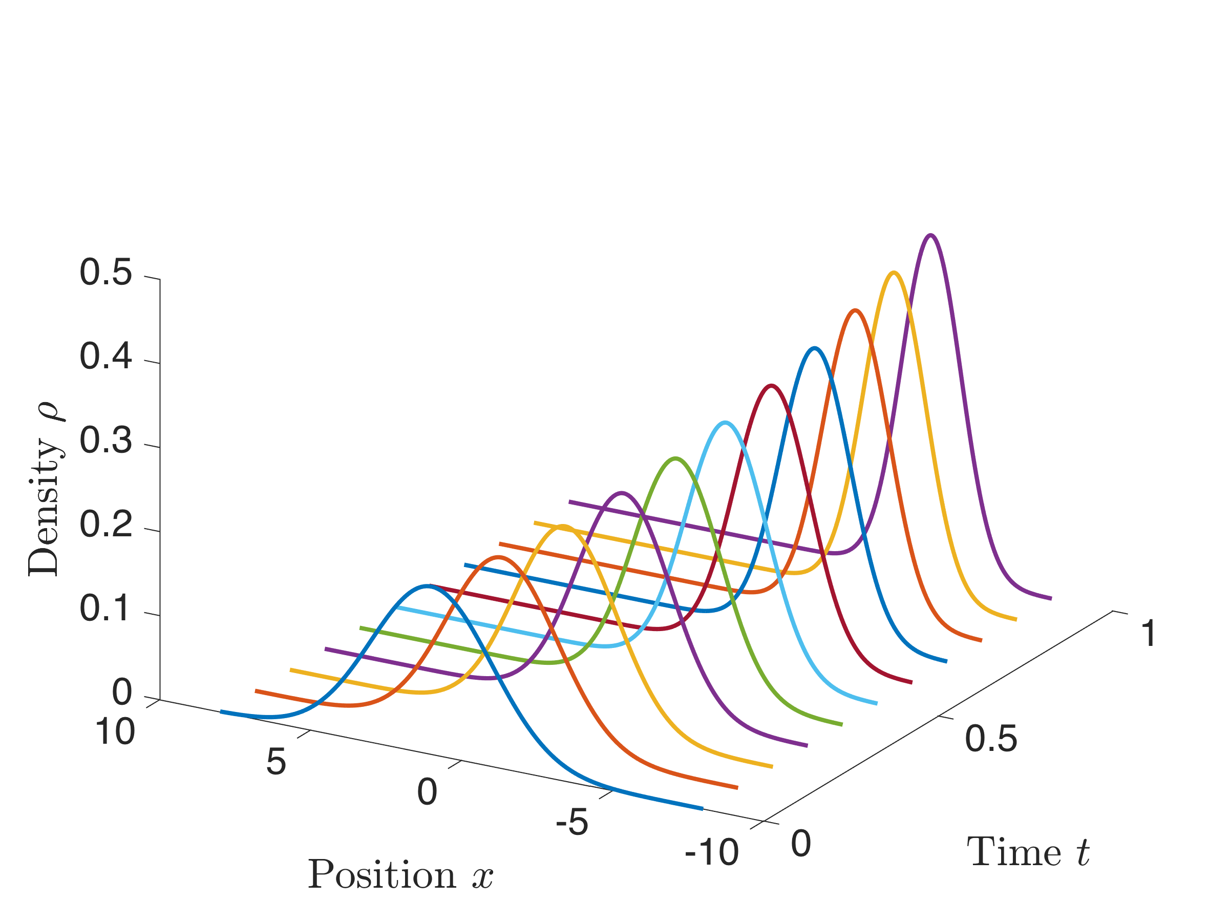
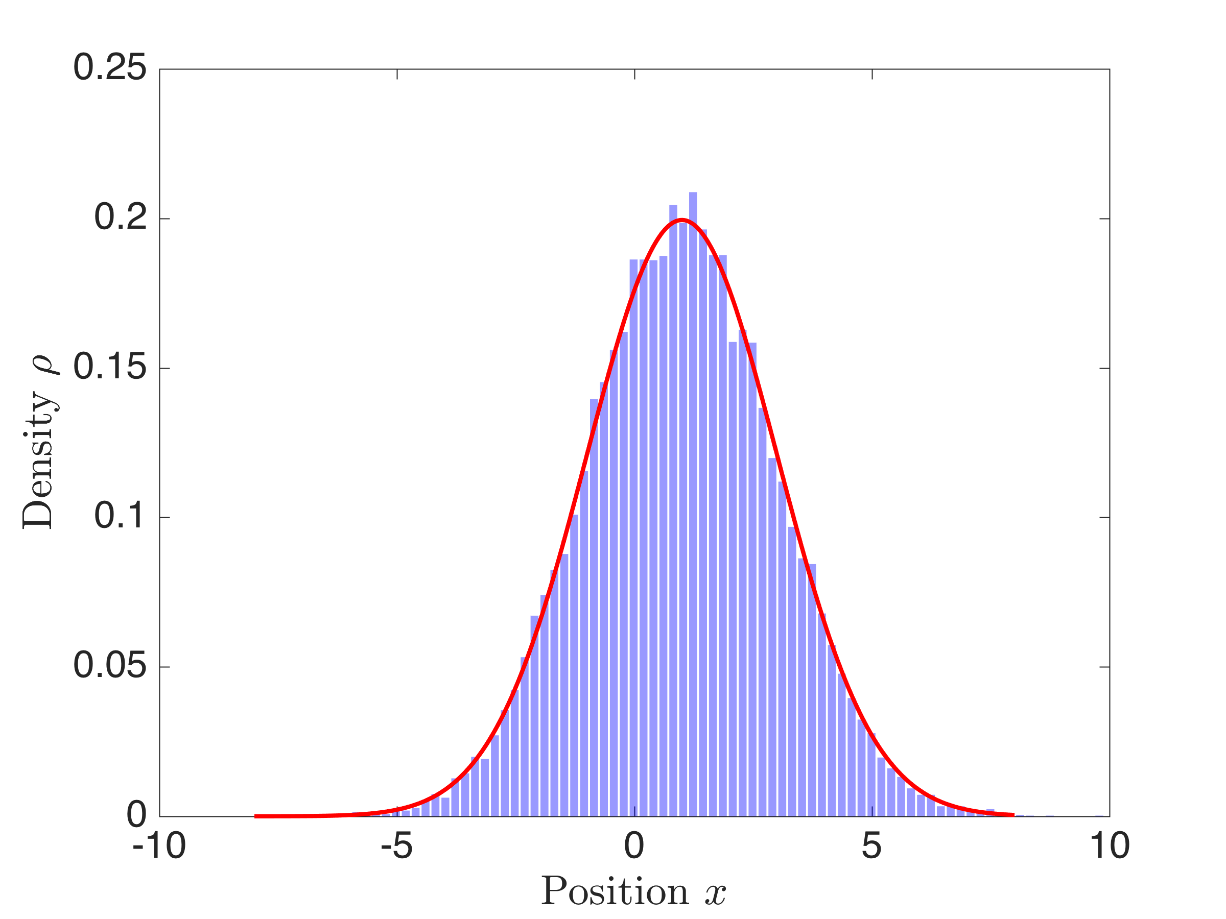
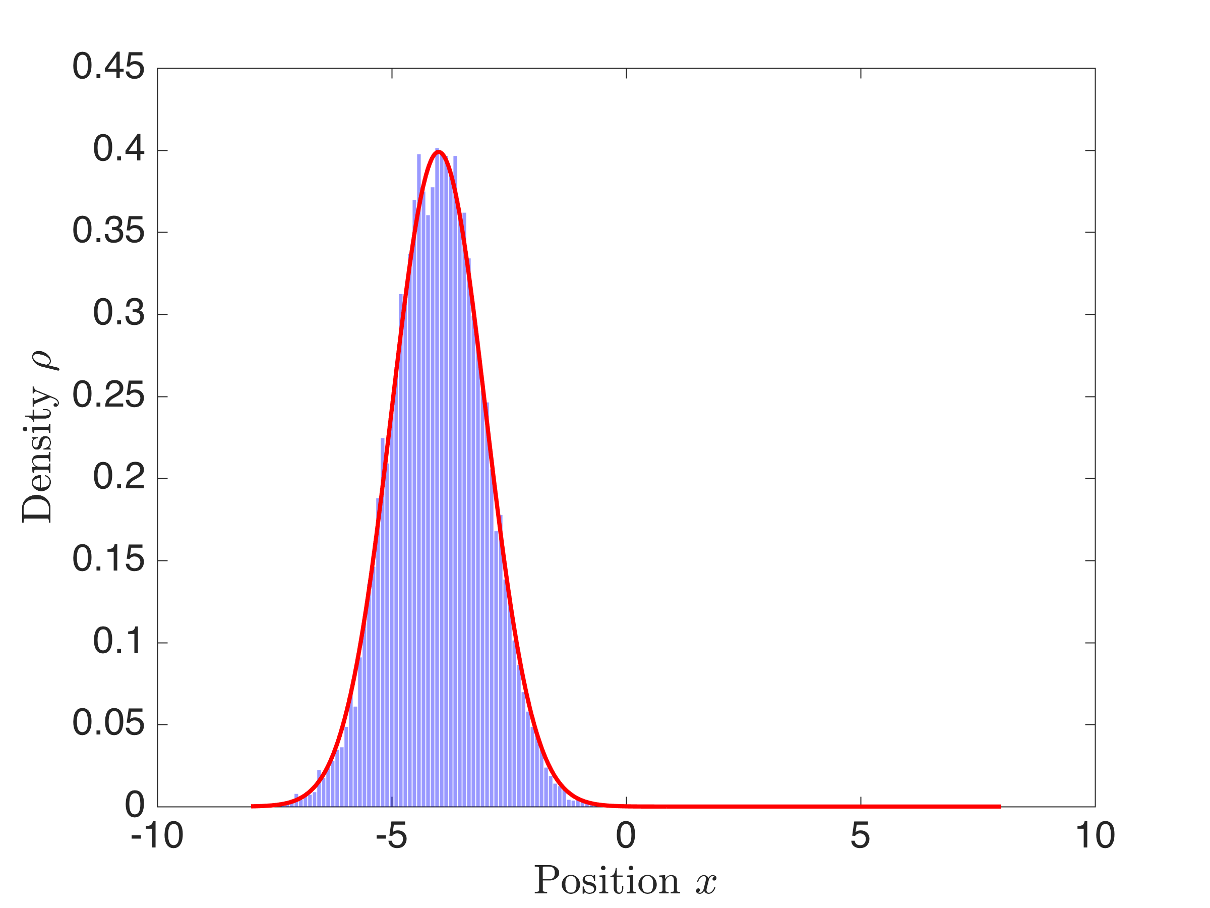
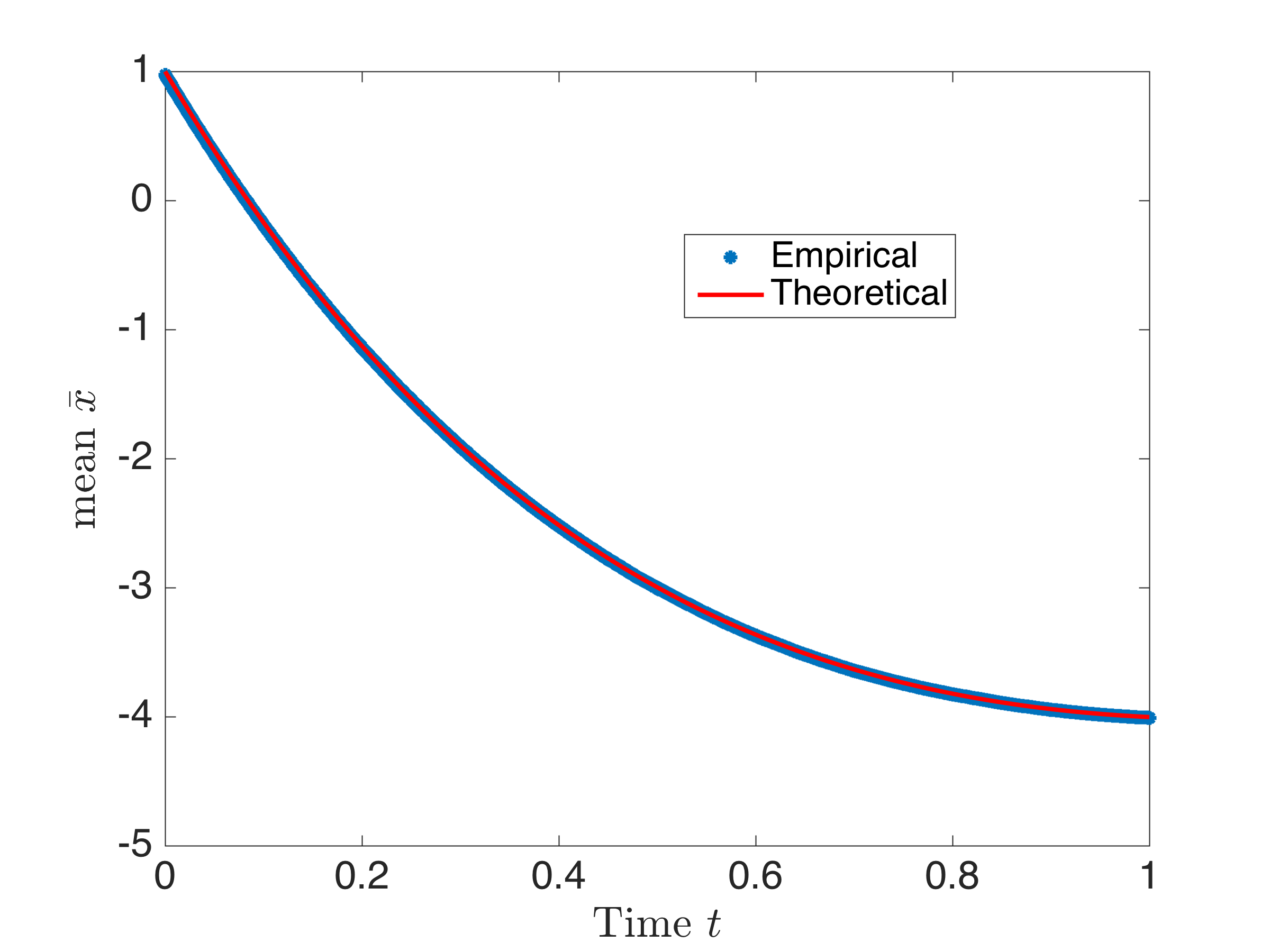
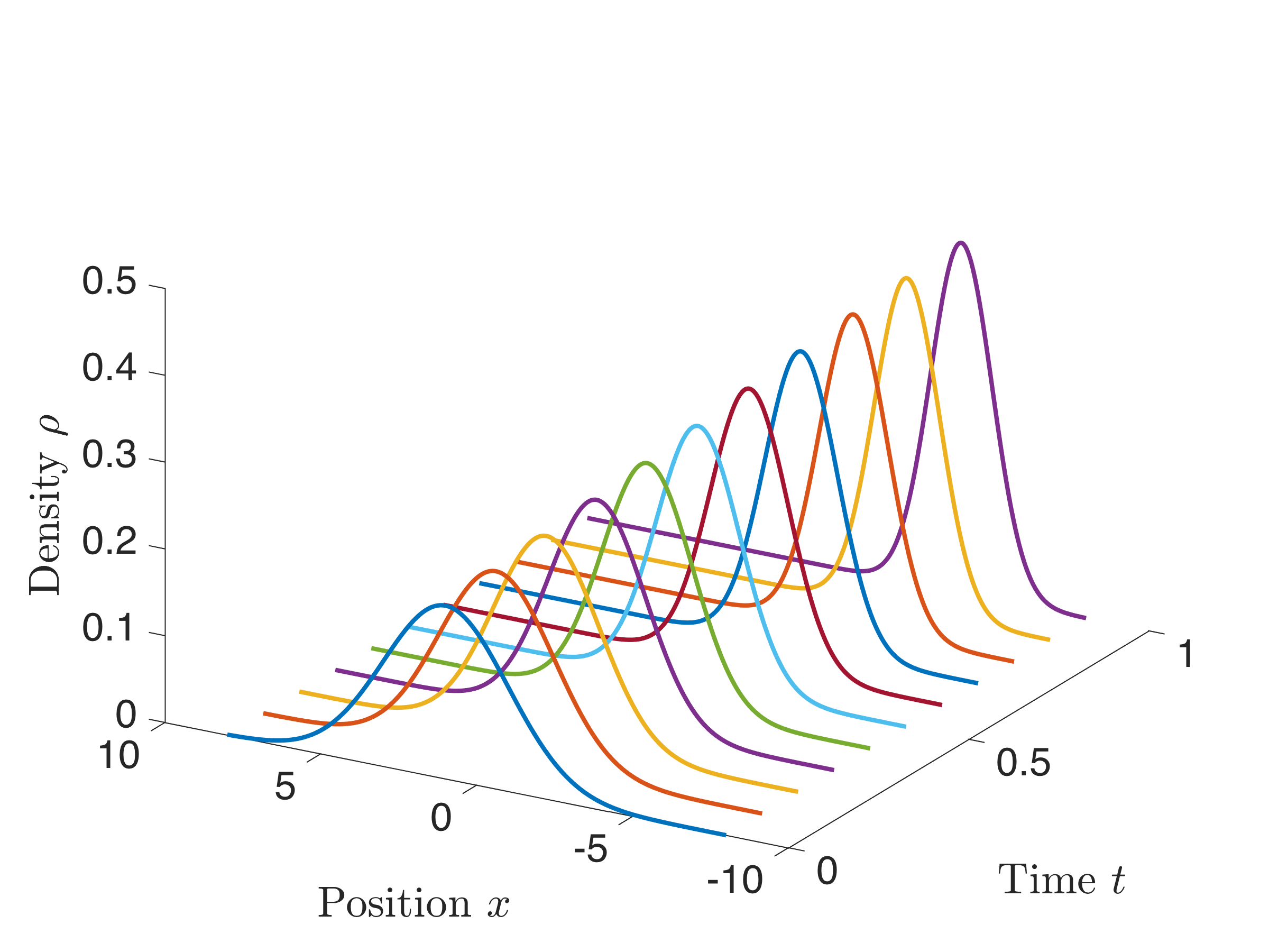
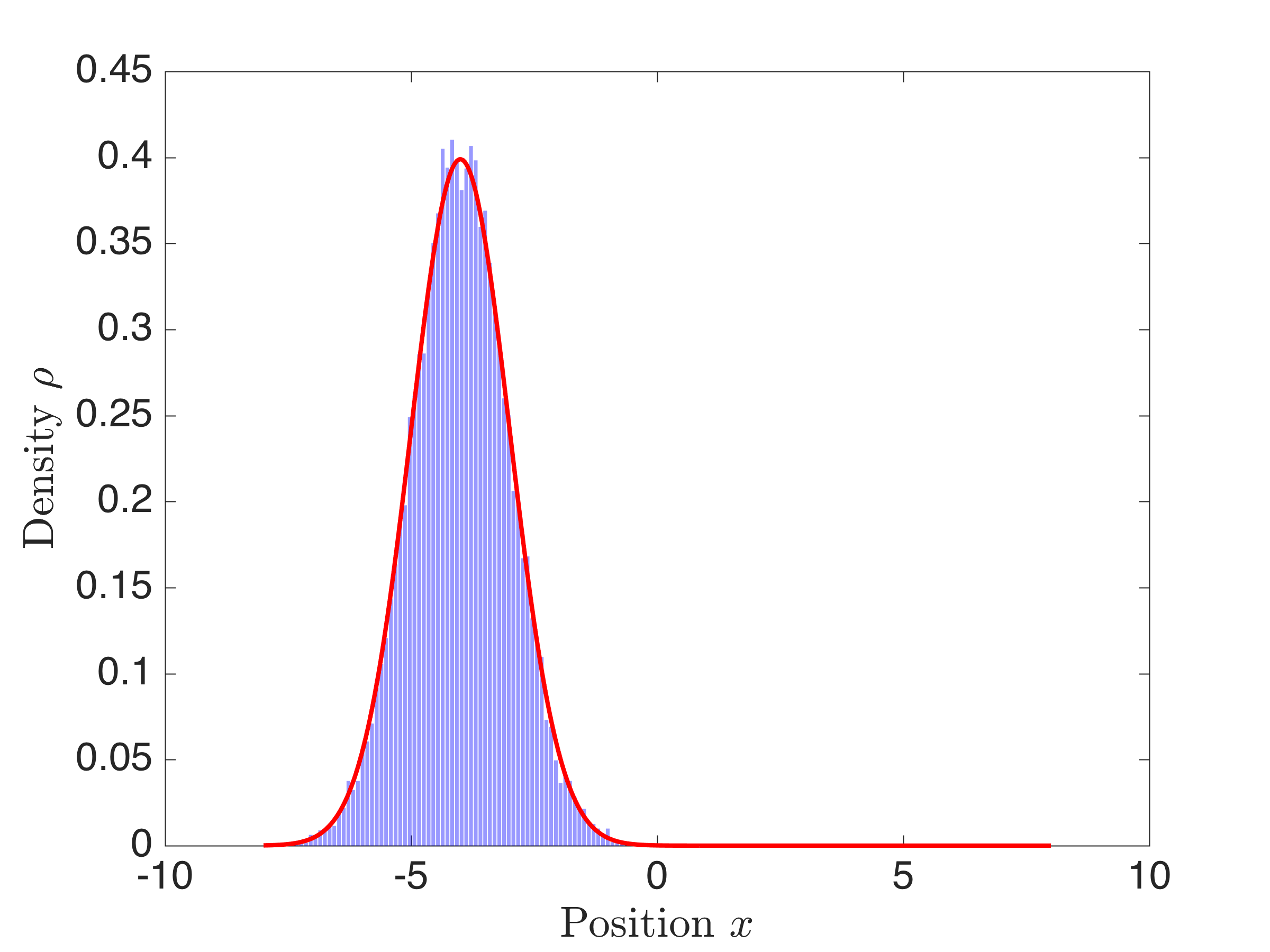
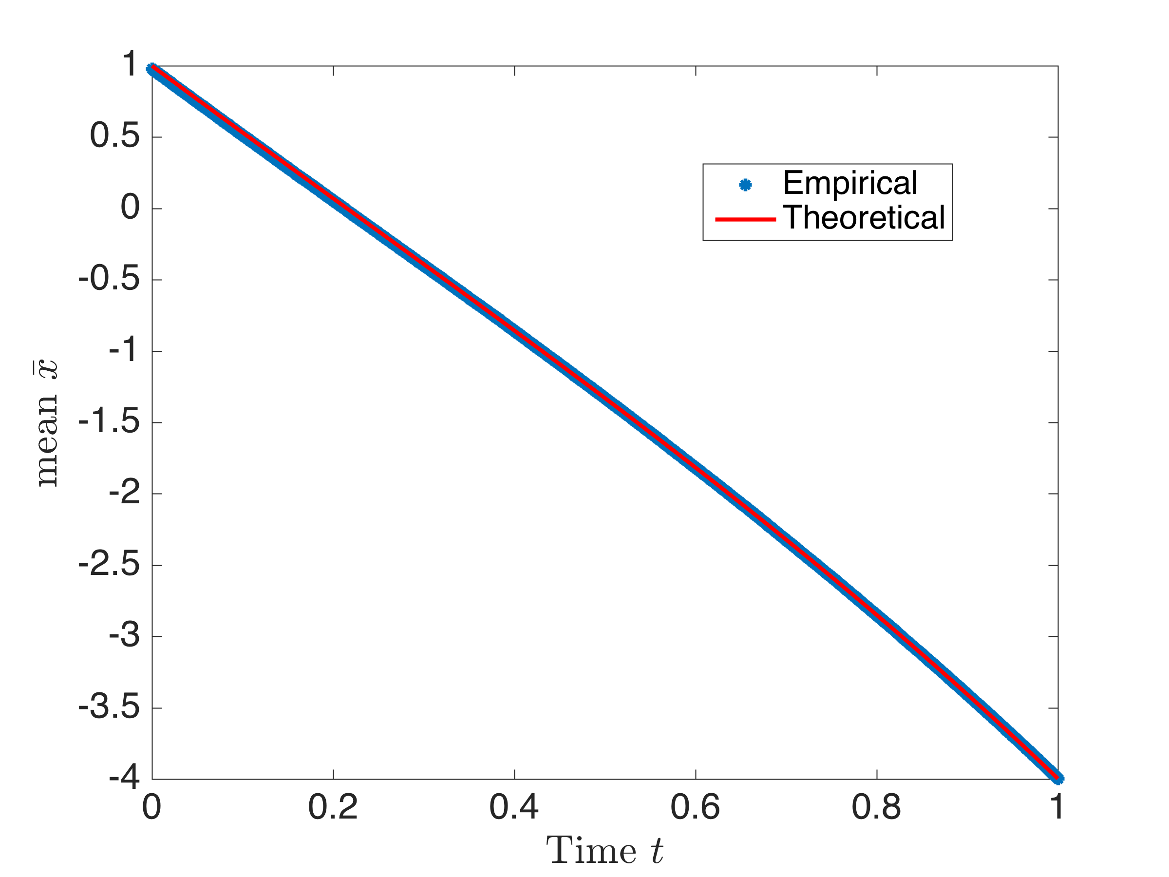
Figure 1 showcases the evolution of the probability density in the Nash equilibrium. To show that the distribution of the agents would evolve according to Figure 1, we simulated the dynamics for a system with $N=20000$ agents under the optimal strategy. Figure 2 and Figure 3 depict the empirical distributions of the particles at time $t=0$ and $t=1$. They match with the theoretical distributions $\rho_{0}$ and $\rho_{1}$ very well. We also show the empirical mean of these particles in Figure 4, which perfectly matches the theoretical result.

Figure 1: Time evolution of probability densities

Figure 2: Empirical distribution of $x(0)$

Figure 3: Empirical distribution of $x(1)$

Figure 4: Time evolution of mean $\bar{x}(t)$

VIII-B Cooperative game

Figure 5 depicts the time evolution of the probability densities with these two marginal distributions in the cooperative game setting. Similarly, we ran some simulations for a particle system with $N=20000$ and obtained Figure 6 and Figure 7 as the empirical distributions of the agents at time $t=0$ and $t=1$. We also show the empirical mean of these particles in Figure 8. Clearly the mean is different to the Nash equilibrium in the noncooperative game setting.

Figure 5: Time evolution of probability densities

Figure 6: Empirical distribution of $x(0)$

Figure 7: Empirical distribution of $x(1)$

Figure 8: Time evolution of mean $\bar{x}(t)$

IX Conclusion

We introduce a paradigm to steer a large number of agents from one distribution to another. The problem lies in the intersection of MFG, OMT and optimal control. We study such problems for linearly weakly interacting agents and solve the problem using tools from all these three areas. Results for several extensions such as stationary and cooperative game problems are also presented. We expect this paradigm to bring in a new dimension to the study and applications of MFG and OMT.

References

• [1] M. Huang, R. P. Malhamé, and P. E. Caines, “Large population stochastic dynamic games: closed-loop mckean-vlasov systems and the nash certainty equivalence principle,” Communications in Information & Systems, vol. 6, no. 3, pp. 221–252, 2006.
• [2] J.-M. Lasry and P.-L. Lions, “Mean field games,” Japanese Journal of Mathematics, vol. 2, no. 1, pp. 229–260, 2007.
• [3] B. Jovanovic and R. W. Rosenthal, “Anonymous sequential games,” Journal of Mathematical Economics, vol. 17, no. 1, pp. 77–87, 1988.
• [4] M. Nourian and P. E. Caines, “ε𝜀\varepsilon-Nash mean field game theory for nonlinear stochastic dynamical systems with major and minor agents,” SIAM Journal on Control and Optimization, vol. 51, no. 4, pp. 3302–3331, 2013.
• [5] R. Carmona, F. Delarue, and A. Lachapelle, “Control of McKean–Vlasov dynamics versus mean field games,” Mathematics and Financial Economics, vol. 7, no. 2, pp. 131–166, 2013.
• [6] M. Huang, P. E. Caines, and R. P. Malhamé, “Individual and mass behaviour in large population stochastic wireless power control problems: centralized and nash equilibrium solutions,” in Decision and Control, 2003. Proceedings. 42nd IEEE Conference on, vol. 1.   IEEE, 2003, pp. 98–103.
• [7] ——, “Large-population cost-coupled LQG problems with nonuniform agents: Individual-mass behavior and decentralized ε𝜀\varepsilon-Nash equilibria,” Automatic Control, IEEE Transactions on, vol. 52, no. 9, pp. 1560–1571, 2007.
• [8] A. Bensoussan, K. Sung, S. C. P. Yam, and S.-P. Yung, “Linear-quadratic mean field games,” Journal of Optimization Theory and Applications, vol. 169, no. 2, pp. 496–529, 2016.
• [9] M. Bardi, “Explicit solutions of some linear-quadratic mean field games,” Networks and Heterogeneous Media, vol. 7, no. 2, pp. 243–261, 2012.
• [10] G. Monge, Mémoire sur la théorie des déblais et des remblais.   De l’Imprimerie Royale, 1781.
• [11] L. V. Kantorovich, “On the transfer of masses,” in Dokl. Akad. Nauk. SSSR, vol. 37, no. 7-8, 1942, pp. 227–229.
• [12] W. Gangbo and R. J. McCann, “The geometry of optimal transportation,” Acta Mathematica, vol. 177, no. 2, pp. 113–161, 1996.
• [13] L. C. Evans, “Partial differential equations and Monge-Kantorovich mass transfer,” Current developments in mathematics, vol. 1997, no. 1, pp. 65–126, 1997.
• [14] L. C. Evans and W. Gangbo, Differential equations methods for the Monge-Kantorovich mass transfer problem.   American Mathematical Soc., 1999, vol. 653.
• [15] C. Villani, Topics in Optimal Transportation.   American Mathematical Soc., 2003, no. 58.
• [16] L. Ambrosio, N. Gigli, and G. Savaré, Gradient flows: in metric spaces and in the space of probability measures.   Springer, 2006.
• [17] C. Villani, Optimal Transport: Old and New.   Springer, 2008, vol. 338.
• [18] L. Ambrosio and N. Gigli, “A user’s guide to optimal transport,” in Modelling and optimisation of flows on networks.   Springer, 2013, pp. 1–155.
• [19] F. Santambrogio, “Optimal transport for applied mathematicians,” Birkäuser, NY, 2015.
• [20] J.-D. Benamou and Y. Brenier, “A computational fluid mechanics solution to the Monge-Kantorovich mass transfer problem,” Numerische Mathematik, vol. 84, no. 3, pp. 375–393, 2000.
• [21] Y. Chen, T. T. Georgiou, and M. Pavon, “On the relation between optimal transport and Schrödinger bridges: A stochastic control viewpoint,” Journal of Optimization Theory and Applications, vol. 169, no. 2, pp. 671–691, 2016.
• [22] ——, “Optimal transport over a linear dynamical system,” IEEE Transactions on Automatic Control, vol. 62, no. 5, pp. 2137–2152, 2017.
• [23] P. Dai Pra, “A stochastic control approach to reciprocal diffusion processes,” Applied mathematics and Optimization, vol. 23, no. 1, pp. 313–329, 1991.
• [24] C. Léonard, “From the Schrödinger problem to the Monge–Kantorovich problem,” Journal of Functional Analysis, vol. 262, no. 4, pp. 1879–1920, 2012.
• [25] ——, “A survey of the Schrödinger problem and some of its connections with optimal transport,” Dicrete Contin. Dyn. Syst. A, vol. 34, no. 4, pp. 1533–1574, 2014.
• [26] I. Gentil, C. Léonard, and L. Ripani, “About the analogy between optimal transport and minimal entropy,” arXiv:1510.08230, 2015.
• [27] Y. Chen, T. T. Georgiou, and M. Pavon, “Optimal steering of a linear stochastic system to a final probability distribution, Part I,” IEEE Trans. on Automatic Control, vol. 61, no. 5, pp. 1158–1169, 2016.
• [28] ——, “Optimal steering of a linear stochastic system to a final probability distribution, Part II,” IEEE Trans. on Automatic Control, vol. 61, no. 5, pp. 1170–1180, 2016.
• [29] M. Fischer, “On the form of the large deviation rate function for the empirical measures of weakly interacting systems,” Bernoulli, vol. 20, no. 4, pp. 1765–1801, 2014.
• [30] P. Cardaliaguet, “Notes on mean field games,” Technical report, Tech. Rep., 2010.
• [31] Y. Chen, “Modeling and control of collective dynamics: From Schrödinger bridges to optimal mass transport,” Ph.D. dissertation, University of Minnesota, 2016.
• [32] Y. Chen, T. T. Georgiou, and M. Pavon, “Optimal steering of a linear stochastic system to a final probability distribution, Part III,” IEEE Trans. on Automatic Control, in print, 2017.
• [33] W. H. Fleming and H. M. Soner, Controlled Markov processes and viscosity solutions.   Springer Science & Business Media, 2006, vol. 25.
• [34] R. Carmona and F. Delarue, “Forward-backward stochastic differential equations and controlled McKean-Vlasov dynamics,” The Annals of Probability, vol. 43, no. 5, pp. 2647–2700, 2015.
• [35] D. A. Dawson and J. Gärtner, “Large deviations from the McKean-Vlasov limit for weakly interacting diffusions,” Stochastics: An International Journal of Probability and Stochastic Processes, vol. 20, no. 4, pp. 247–308, 1987.
• [36] J. Feng and T. G. Kurtz, Large deviations for stochastic processes.   American Mathematical Society Providence, 2006, vol. 131.