Entanglement hamiltonian and entanglement contour in inhomogeneous 1D critical systems

Abstract

Inhomogeneous quantum critical systems in one spatial dimension have been studied by using conformal field theory in static curved backgrounds. Two interesting examples are the free fermion gas in the harmonic trap and the inhomogeneous XX spin chain called rainbow chain. For conformal field theories defined on static curved spacetimes characterised by a metric which is Weyl equivalent to the flat metric, with the Weyl factor depending only on the spatial coordinate, we study the entanglement hamiltonian and the entanglement spectrum of an interval adjacent to the boundary of a segment where the same boundary condition is imposed at the endpoints. A contour function for the entanglement entropies corresponding to this configuration is also considered, being closely related to the entanglement hamiltonian. The analytic expressions obtained by considering the curved spacetime which characterises the rainbow model have been checked against numerical data for the rainbow chain, finding an excellent agreement.

Contents

1 Introduction

Entanglement has become a central tool to study extended quantum systems in different areas of theoretical physics such as condensed matter physics, quantum information theory, quantum optics and quantum gravity [1]. Recent important advances have allowed to set up experiments which have detected characteristic features of entanglement [2].

Entanglement in spatially inhomogeneous systems has attracted a lot of attention. Indeed, being inhomogeneity ubiquitous in experimental settings, it is important to assess the validity of the predicted universal features of entanglement in inhomogeneous systems. For instance, quenched disorder in the coupling constants of a critical system in one spatial dimension can lead to a behavior which is remarkably similar to the conformal case, with a logarithmic growth of the average block entropies [3, 4]. Other interesting inhomogeneous systems in one spatial dimension are fermionic systems in the presence of a trapping potential [5, 6], spin chains with gradients [7], spin chains with exponential growth of the couplings near the edges in order to reduce the boundary effects [8] and the rainbow chain, where exponentially reduced couplings towards the endpoints of a segment lead to a volumetric growth of the entanglement entropy in the ground state [9, 10, 11, 12, 13].

The rainbow chain can be considered as the vacuum of a quantum field theory on a curved background with negative curvature [13]. Interestingly, the ground state of the rainbow chain in a particular limit resembles a thermofield double state, i.e. each half of the chain behaves like a homogeneous system at a finite temperature [11].

Other interesting models have been considered in [14]. The similarity between smoothly inhomogeneous couplings and the occurrence of a static curved background metric has been employed to design simulators for effects which are characteristic of quantum field theory in curved spacetimes, such as the Unruh effect [15].

The entanglement entropies, i.e. the entanglement entropy and the Rényi entropies, are important quantities to study in order to quantify the bipartite entanglement [16, 17, 18, 19]. Other quantities can be introduced which are expected to provide more information about the entanglement of a bipartition. In particular, in this manuscript we consider the entanglement hamiltonian [21, 22, 23, 24, 25], an operator whose spectrum gives the entanglement entropy and the Rényi entropies, and the contour for the entanglement entropies [26, 27, 28, 29]. Our goal is to study quantitatively these magnitudes for some inhomogeneous critical systems in one spatial dimension. The rainbow model is the main benchmark of our analysis.

Given a quantum system in its ground state $|\Psi\rangle$ and a spatial bipartition of the system into two subsystems $A$ and $B$ such that $A\cup B$ is the entire space, one can assume that, correspondingly, the Hilbert space of the system can be factorised as $\mathcal{H}=\mathcal{H}_{A}\otimes\mathcal{H}_{B}$. The reduced density matrix $\rho_{A}\equiv{\rm Tr}_{B}|\Psi\rangle\langle\Psi|$ associated to the subsystem $A$ is obtained by tracing over the degrees of freedom of $B$ and it can always be written as

$$\rho_{A}=e^{-2\pi K_{A}}\,,$$ (1)

where the operator $K_{A}$ is the entanglement hamiltonian. After the seminal work of Bisognano and Wichmann [21], several interesting quantitative results have been obtained about the explicit form of $K_{A}$ in quantum field theories [22, 24]. The entanglement hamiltonian has been studied also in some lattice models [23, 25]. The entanglement spectrum is given by the eigenvalues of $\rho_{A}$ [30, 31].

The Rényi entropies are important scalar quantities defined from the $n$-th power of the reduced density matrix as follows

$$S^{(n)}_{A}\,=\,\frac{1}{1-n}\,\log{\rm Tr}\rho^{n}_{A}\,,$$ (2)

where $n\geqslant 2$ is an integer parameter. The entanglement entropy can be found from the Rényi entropies (2) through the replica limit $S_{A}=\lim_{n\rightarrow 1}S^{(n)}_{A}$, which requires to perform an analytic continuation of the integer parameter $n$. In the following we denote by $S^{(n)}_{A}$ with $n\geqslant 1$ the entanglement entropies, meaning that $S^{(1)}_{A}\equiv S_{A}$. An important property to remind is $S^{(n)}_{A}=S^{(n)}_{B}$ for any $n\geqslant 1$ when the entire system is in a pure state. It is worth remarking that the entanglement entropies are scalar quantities which can be constructed from the entanglement spectrum.

Another interesting quantity to consider is the contour for the entanglement entropies [26, 27, 28, 29]. In a lattice model where a spatial bipartition has been introduced, the contour for the entanglement entropies is given by a non negative function $s_{A}^{(n)}(i)$ (called contour function in the following) which provides information about the contribution of the $i$-th site in $A$ to the entanglement between $A$ and $B$. The minimal properties that the contour function must satisfy are

$$S_{A}^{(n)}=\sum_{i\,\in\,A}s_{A}^{(n)}(i)\,,\;\;\qquad\;\;s_{A}^{(n)}(i)\geqslant 0\,.$$ (3)

It is straightforward to observe that these two conditions do not define the contour function $s_{A}^{(n)}(i)$ in a unique way. The simplest function fulfilling (3) is the flat contour $s_{A}^{(n)}(i)=S_{A}^{(n)}/|A|$, where $|A|$ is the total number of sites in $A$. Nonetheless, we do not expect that all the sites in $A$ equally contribute to $S_{A}^{(n)}$. Indeed, the main contribution should come from the sites near the hypersurface separating $A$ and $B$ (often called entangling hypersurface). In order to improve the definition of the contour for the entanglement entropies, further requirements have been introduced in [27], where an explicit construction of $s_{A}^{(n)}(i)$ for free fermions on the lattice has been proposed. In harmonic lattices, a contour function $s_{A}^{(n)}(i)$ satisfying (3) and other properties close to the ones introduced in [27] has been constructed in [29] (see also [26, 28] for previous work). The CFT description of the contour for the entanglement entropies has been discussed in [29], by employing the analysis of [24]. We remark that, while the entanglement spectrum provides all the entanglement, further information is required to construct the contour for the entanglement entropies.

In this manuscript we consider quantum systems on a one dimensional (1D) lattice whose continuum limit is described by conformal field theories (CFTs). Thus, the complementary domains $A$ and $B$ are made by intervals and the entangling hypersurface by isolated points. In $1+1$ dimensional quantum field theories ${\rm Tr}\rho_{A}^{n}$ can be computed through the replica construction by considering $n$ copies of the underlying model and joining them cyclically in a proper way. An ultraviolet (UV) cutoff $\epsilon$ is needed to regularize the ultraviolet divergencies. Following [17], in the two dimensional Euclidean spacetime where the field theory is defined, the UV cutoff can be introduced by removing infinitesimal disks of radius $\epsilon$ centered at the entangling points separating $A$ and $B$. In [24] this regularization procedure has been adopted to study the entanglement hamiltonian $K_{A}$ for certain configurations. This approach is adopted also in our analysis.

Alternatively, ${\rm Tr}\rho_{A}^{n}$ can be computed as correlation functions of twist fields located at the entangling points [19, 20]. In this approach the UV cutoff is introduced through a thin slit of width $\epsilon$ separating the upper and the lower edge of $A$ in the direction of the euclidean time. This method has been employed also for the entanglement entropies of subsystems made by disjoint intervals [32].

In this manuscript we study the entanglement hamiltonian and the contour function for the entanglement entropies corresponding to a particular configuration in 1D inhomogeneous critical systems. In particular, the system is defined on a segment where the same boundary condition is imposed at the endpoints and the subsystem $A$ is an interval adjacent to one of the boundaries. Analytic results are obtained which are valid for a large class of inhomogeneous critical systems in 1D. The benchmark for our analytic expressions is the rainbow model. A numerical analysis is performed for this inhomogeneous critical chain by adapting the method of [33] for the entanglement hamiltonian and the method of [27] for the contour function for the entanglement entropies. An excellent agreement is found between the lattice data and the corresponding analytic formulas in the continuum.

The manuscript is organized as follows. In §2 we review the results for the homogenous systems that will be extended to inhomogeneous systems, namely some results of [24] for the entanglement hamiltonian and of [29] for the contour function. The rainbow chain is briefly introduced in §3. In §4 we review the results of [6, 13] about the entanglement entropies in inhomogeneous 1D free fermionic systems for an interval adjacent to the boundary of a finite segment, obtained through the twist field method. Focussing on this configuration in the continuum limit of inhomogeneous 1D critical systems, we construct the corresponding entanglement hamiltonian and entanglement spectrum in §5, and in §6 we provide the corresponding contour for the entanglement entropies. In §7 the analytic formulas derived in the previous sections are specified for the rainbow model and checked against numerical data obtained for rainbow chains by adapting the methods of [33] and [27] to this inhomogeneous system. Conclusions are drawn in §8, where some open directions for future work are also discussed.

2 Entanglement hamiltonian and contour in homogenous systems

In this section we review the results of [24] that are needed in the subsequent analysis.

Considering a subsystem $A$ made by an interval of finite length in a larger system which can have either infinite or finite size, the UV regularization of the path integral in the corresponding euclidean spacetime can be performed by removing infinitesimal circles of radius $\epsilon$ around the entangling points, namely the endpoints of $A$ and $B$ which separates $A$ from $B$. The analysis of [24] is valid in CFT and only for certain configurations where $A$ has either one or two entangling points. In the former case, the interval ends on the physical boundary of the whole system.

Once the UV regularization has been introduced, the configurations considered in [24] are such that one can construct a conformal map which sends the spacetime obtained after the removal of the infinitesimal disks (parameterised by the complex coordinate $z$) into an annulus described by another complex coordinate $w=f(z)$. This annulus is a rectangle whose width is $2\pi$ in the ${\rm Im}\,w$ direction and $W_{A}$ in the ${\rm Re}\,w$ direction, where the annular structure is given by the identification ${\rm Im}\,w\sim{\rm Im}\,w+2\pi$. A crucial role is played by the width $W_{A}$ of the annulus, which is provided by the conformal map $f(z)$ as follows

$$W_{A}=\int_{A_{\epsilon}}f^{\prime}(x)\,dx\,,$$ (4)

where $A_{\epsilon}$ corresponds to the interval left after the removal of the infinitesimal disks around the entangling points. The width $W_{A}$ coincides with the difference between the values of $f(x)$ at the endpoints of $A_{\epsilon}$ and it diverges logarithmically as $\epsilon\to 0$. For instance, when $A=(u,v)$ is an interval of length $\ell=v-u$ on the infinite line, we have that $A_{\epsilon}=(u+\epsilon\,,v-\epsilon)$ and $W_{A}=2\log(\ell/\epsilon)+O(\epsilon)$.

The entanglement hamiltonian $K_{A}$ for the static configurations considered in [24] can be written in terms of the conformal map $f(z)$ as follows

$$K_{A}=\int_{A}\frac{T_{00}(x)}{f^{\prime}(x)}\,dx\,,$$ (5)

where $T_{00}=T+\overline{T}$ is a specific component of the energy-momentum tensor of the underlying CFT. This leads to express the trace of the $n$-th power of the reduced density matrix as

$${\rm Tr}\,\rho^{n}_{A}\,=\,e^{-2\pi nK_{A}}\,=\,\frac{\mathcal{Z}_{n\textrm{\tiny-annulus}}}{\mathcal{Z}_{\textrm{\tiny annulus}}^{n}}\,,$$ (6)

where $\mathcal{Z}_{n\textrm{\tiny-annulus}}$ is the partition function of the underlying CFT where the worldsheet is an annulus similar to the one introduced above. In particular, the $n$-annulus is a rectangle whose width is again $W_{A}$ in the ${\rm Re}\,w$ direction, but the width in the ${\rm Im}\,w$ direction is $2\pi n$. Thus, the identification ${\rm Im}\,w\sim{\rm Im}\,w+2\pi n$ is imposed for the $n$-annulus. The boundary conditions are the same for both the annular partition functions occurring in (6).

In the construction of [24], the entanglement entropies can be written in terms of the width $W_{A}$ as follows

$$S^{(n)}_{A}=\frac{c}{12}\left(1+\frac{1}{n}\right)W_{A}+C_{n}+o(1)\,,$$ (7)

where $c$ is the central charge of the CFT and $C_{n}$ is a constant depending on the boundary entropies introduced through the regularisation procedure and therefore on the microscopic details of the model. We remark that the well known logarithmic divergence of $S^{(n)}_{A}$ as $\epsilon\to 0$ comes from $W_{A}$. The analysis of [24] has access only to universal features; therefore the $n$ dependence of the non universal constant $C_{n}$ cannot be addressed.

In [24] also the eigenvalues $\lambda_{j}$ of the reduced density matrix $\rho_{A}$ have been found. They are given by

$$\lambda_{j}=\frac{q^{-c/24+\Delta_{j}}}{\mathcal{Z}_{\textrm{\tiny annulus}}}=\frac{q^{-c/24+\Delta_{j}}}{\langle a|0\rangle\langle 0|b\rangle\,\tilde{q}^{\,-c/24}}\,\big(1+\dots\big)\,,$$ (8)

where the modular parameters of the flat annulus read

$$q\equiv e^{-2\pi^{2}/W_{A}}\,,\qquad\tilde{q}\equiv e^{-2W_{A}}\,,$$ (9)

and $\Delta_{j}$ are the dimensions of the boundary operators consistent with the boundary conditions at the edges of the annulus, which are characterised by the boundary states $|a\rangle$ and $|b\rangle$. The dots in (8) correspond to subleading terms as $\epsilon\to 0$. In the intermediate step of (8), the denominator $\mathcal{Z}_{\textrm{\tiny annulus}}$ is the partition function of the underlying CFT on the flat annulus. From (8) and (9) one easily obtains that

$$-\log\lambda_{j} = -\left(\Delta_{j}-\frac{c}{24}\,\right)\log q+\log\mathcal{Z}_{\textrm{\tiny annulus}}$$ (10)

$$= \frac{c}{12}\,W_{A}+\log\big(\langle a|0\rangle\langle 0|b\rangle\big)+\left(\Delta_{j}-\frac{c}{24}\right)\frac{2\pi^{2}}{W_{A}}+O(\epsilon^{r})\,,$$ (11)

where $r>0$. Taking the limit $n\to 1$ of (7), one finds that the entanglement entropy at leading order is given by $S_{A}=c\,W_{A}/6$. Comparing this result with the expansion (11), it is straightforward to observe that $-\log\lambda_{j}=S_{A}/2$ for any eigenvalue at leading order.

The largest eigenvalue corresponds to $\Delta_{j}=0$, therefore we have

$$-\log\lambda_{\textrm{\tiny max}}\,=\,\frac{c}{12}\,W_{A}+\log\big(\langle a|0\rangle\langle 0|b\rangle\big)-\frac{\pi^{2}c}{12\,W_{A}}+O(\epsilon^{r})\,,$$ (12)

which tells us that the leading divergence of the maximum eigenvalue provides the central charge, while the subleading one contains the boundary conditions. The largest eigenvalue $\lambda_{\textrm{\tiny max}}$ gives the single-copy entanglement and the relation $-\log\lambda_{\textrm{\tiny max}}=S_{A}/2$ in this case is well known [30].

We find it worth introducing the following gaps

$$\log\lambda_{j}-\log\lambda_{k}=\frac{2\pi^{2}}{W_{A}}\,(\Delta_{k}-\Delta_{j})\,,$$ (13)

where the r.h.s. has been obtained from (10) and therefore it includes all orders corrections in $\epsilon$. Considering the largest eigenvalue $\lambda_{j}=\lambda_{\textrm{\tiny max}}$ and adopting the shorthand notation $\mathcal{E}_{k}\equiv\log\lambda_{\textrm{\tiny max}}-\log\lambda_{k}$, we get

$$\mathcal{E}_{k}=\frac{2\pi^{2}\Delta_{k}}{W_{A}}\,.$$ (14)

We find it worth observing that, from (7) and (14) we obtain

$$S^{(n)}_{A}\,\mathcal{E}_{k}\,=\,\frac{\pi^{2}}{6}\left(1+\frac{1}{n}\,\right)\Delta_{k}+\dots\,,$$ (15)

where the dots denote infinitesimal terms as $\epsilon\to 0$.

The above discussion applies to all the static configurations such that the euclidean spacetime obtained after the removal of the regularization disks around the entangling point(s) can be mapped into an annulus [24].

By plugging (4) into (7), it is straightforward to find that the entanglement entropies for the static configurations considered in [24] can be written as

$$S_{A}^{(n)}=\int_{A_{\epsilon}}s_{A}^{(n)}(x)\,dx\,,\;\;\qquad\;\;s_{A}^{(n)}(x)\geqslant 0\,,$$ (16)

where

$$s_{A}^{(n)}(x)=\frac{c}{12}\left(1+\frac{1}{n}\right)f^{\prime}(x)+\frac{C_{n}}{\ell}\,.$$ (17)

In [29] this expression has been proposed as the continuum limit of the contour function for the entanglement entropies in CFTs for the static configurations discussed in [24].

In this manuscript we focus on the case where $A$ is an interval of length $\ell$ adjacent to the boundary of the segment $(-L,L)$, where the same boundary condition is imposed at the endpoints, which is among the ones considered in [24] (comparing to the notations, we have that $2L=L_{\textrm{\tiny there}}$). We can set $A=(x_{0},L)$ and only one entangling point occurs.

For this configuration we have to consider the euclidean spacetime given by the strip $\mathbb{S}=\{(x,t_{\textrm{\tiny E}})\in(-L,L)\times\mathbb{R}\}$, which will be parameterised by the complex coordinate $z=x+\textrm{i}t_{\textrm{\tiny E}}$ in the following. The UV regularization employed in [17, 24] requires to remove the infinitesimal disk $\mathbb{D}_{\epsilon}(x_{0})=\{|z-x_{0}|\leqslant\epsilon\}$ of radius $\epsilon$ centered at the entangling point $z=x_{0}$. The resulting spacetime $\mathbb{S}\setminus\mathbb{D}_{\epsilon}(x_{0})$ is shown in the left panel of Fig. 1. This regularization procedure naturally leads to introduce the regularised intervals $A_{\epsilon}\equiv(x_{0}+\epsilon,L)$ and $B_{\epsilon}\equiv(-L,x_{0}-\epsilon)$.

Figure 1: Euclidean spacetimes describing the case of an interval $A=(x_{0},L)$ of length $\ell=L-x_{0}$ in the segment $(-L,L)$. In the left panel a small disk $\mathbb{D}_{\epsilon}(x_{0})$ of radius $\epsilon$ centered at the entangling point $x_{0}$ has been removed from the strip $\mathbb{S}=\{(x,t_{\textrm{\tiny E}})\in(-L,L)\times\mathbb{R}\}$, where the same boundary condition is imposed on the boundaries (solid black lines). The sequence $z\to\xi\to\zeta\to w$ of conformal transformations allows to construct the conformal map (20), which sends the spacetime $\mathbb{S}\setminus\mathbb{D}_{\epsilon}(x_{0})$ (left panel) into the annulus $\mathbb{A}$ shown in the right bottom panel, where the horizontal segment at $\textrm{Im}\,w=0$ and the one at $\textrm{Im}\,w=2\pi$ delimiting the spacetime in the vertical direction must be identified. The width $W_{A}$ of the annulus $\mathbb{A}$ is given by (23).

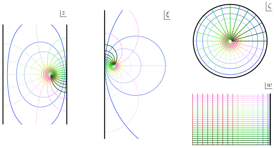
The conformal map $w=f(z)$ which sends the holed strip $\mathbb{S}\setminus\mathbb{D}_{\epsilon}(x_{0})$ into the annulus (right bottom panel in Fig. 1) can be constructed through the following intermediate steps. First one maps the strip $\mathbb{S}$ into the right half plane (middle panel in Fig. 1) through the conformal transformation $z\to\xi=e^{\textrm{i}\pi z/(2L)}$. The entangling point $x_{0}$ is mapped into $\xi_{0}\equiv\xi(x_{0})$. Then, the resulting spacetime can be mapped into the circular crown $\mathbb{D}_{1}\setminus\mathbb{D}_{R}$ (right top panel in Fig. 1), being $\mathbb{D}_{1}=\{\zeta,|\zeta|\leqslant 1\}$ the unit disk and $\mathbb{D}_{R}=\{\zeta,|\zeta|\leqslant R\}$ the infinitesimal disk of radius $R$ centered in the origin. The conformal map $\xi\to\zeta(\xi)$ implementing this transformation must send $\xi_{0}$ into the origin. It reads [34, 24]

$$\zeta(z)=-\,\textrm{i}\,\frac{(1+\bar{\xi}_{0})(\xi-\xi_{0})}{(1+\xi_{0})(\xi+\bar{\xi}_{0})}=\frac{\sin(\pi(z-x_{0})/(4L))}{\cos(\pi(z+x_{0})/(4L))}\,.$$ (18)

The boundaries of $\mathbb{S}$, which have $x=-L$ and $x=L$, are sent into the boundary of $\mathbb{D}_{1}$, which is the circumference $|\zeta|=1$. The disk $\mathbb{D}_{\epsilon}(x_{0})\subset\mathbb{S}$ is mapped into the disk $\mathbb{D}_{R}\subset\mathbb{D}_{1}$ centered in the origin whose radius is infinitesimal as $\epsilon\to 0$; indeed

$$R\simeq\frac{\pi\epsilon/(4L)}{\cos(\pi x_{0}/(2L))}=\frac{\pi\epsilon/(4L)}{\sin(\pi\ell/(2L))}\,,$$ (19)

being $\ell=L-x_{0}$ the length of the interval $A$. The intervals $A$ and $B$ are mapped into the segments $(R,1)$ and $(-1,-R)$ respectively.

Finally, the conformal transformation $w=f(z)$ is given by [24]

$$w=f(z)=\log\big(\zeta(z)\big)=\log\left(\frac{\sin(\pi(z-x_{0})/(4L))}{\cos(\pi(z+x_{0})/(4L))}\right),$$ (20)

which sends $\mathbb{S}\setminus\mathbb{D}_{\epsilon}(x_{0})$ into the annulus $\mathbb{A}=(\log R,0)\times[0,2\pi)$, where ${\rm Im}\,w=0$ is identified with ${\rm Im}\,w=2\pi$ (see the right bottom panel in Fig. 1). The regularised interval $A_{\epsilon}$ is mapped into the interval $[\log R,0]$ on the negative real axis, while the block $B_{\epsilon}$ lies in the center of the annulus having ${\rm Im}\,w=\pi$.

The general expressions discussed above for the entanglement hamiltonian, the entanglement spectrum and the contour for the entanglement entropies can be specified to this configuration by employing the map (20). In this case the boundary states $|a\rangle$ and $|b\rangle$ encode the two (maybe different) boundary conditions that must be specified: along the vertical lines, which correspond to the physical boundary of the segment, and along the boundary of the infinitesimal disk $\mathbb{D}_{\epsilon}(x_{0})$ centered at the entangling point.

The weight function to employ in the expression (5) of the entanglement hamiltonian for this configuration can be easily obtained from (20). It reads

$$\frac{1}{f^{\prime}(x)}\,=\,\frac{2L}{\pi}\;\frac{\sin(\pi x/(2L))-\sin(\pi x_{0}/(2L))}{\cos(\pi x_{0}/(2L))}\,.$$ (21)

From this formula it is straightforward to notice that $f^{\prime}(x)>0$ for $x\in A$.

The expansion of this weight function as $x\to x_{0}$ is given by

$$\frac{1}{f^{\prime}(x)}=(x-x_{0})-\frac{\pi\tan(\pi x_{0}/(2L))}{4L}\,(x-x_{0})^{2}+O\big((x-x_{0})^{3}\big)\,.$$ (22)

The leading term corresponds to the expected behavior dictated by the Bisognano-Wichmann theorem for a semi-infinite line [21]. As for the subleading $O((x-x_{0})^{2})$ term, its sign is opposite to the sign of $x_{0}$; therefore when $x\simeq x_{0}^{+}$ we have that the curve (22) is above the one provided by the Bisognano-Wichmann result for $x_{0}<0$, while it stays below for $x_{0}>0$.

From (20), we have that the width of the $\mathbb{A}$ (right bottom panel of Fig. 1) is [24]

$$W_{A}=f(L)-f(x_{0}+\epsilon)=-\log R=\log\left[\frac{4L}{\pi\epsilon}\sin\left(\frac{\pi\ell}{2L}\right)\right]+O(\epsilon)\,.$$ (23)

By employing this result into (7) we obtain the entanglement entropies

$$S^{(n)}_{A}=\frac{c}{12}\left(1+\frac{1}{n}\right)\log\left[\frac{4L}{\pi\epsilon}\sin\left(\frac{\pi\ell}{2L}\right)\right]+C_{n}+o(1)\,.$$ (24)

For this configuration the gaps (14) become

$${\cal E}_{k}=\frac{2\pi^{2}\Delta_{k}}{\log\big[\tfrac{4L}{\pi\epsilon}\,\sin(\tfrac{\pi\ell}{2L})\big]}\,.$$ (25)

As consistency check, notice that for $A$ given by half system (i.e. $\ell=L$) one recovers the well known scaling dependence $1/\log L$ [23, 35].

Finally, let us write explicitly also the contour function for the entanglement entropies corresponding to this configuration, which can be easily obtained from (17) and (21). The result is

$$s_{A}^{(n)}(x)=\frac{c}{12}\left(1+\frac{1}{n}\right)\frac{\pi}{2L}\;\frac{\cos(\pi x_{0}/(2L))}{\sin(\pi x/(2L))-\sin(\pi x_{0}/(2L))}+\frac{C_{n}}{\ell}\,.$$ (26)

From (22), we have that $s_{A}^{(n)}(x)=\tfrac{c}{12}(1+\tfrac{1}{n})/(x-x_{0})+\dots$ as $x\to x_{0}^{+}$. Instead, it is straightforward to notice $s_{A}^{(n)}(L)$ is finite. We remark that the product $L\,s_{A}^{(n)}(x)$ is a function of $x/L$ parameterised by $n$ and $x_{0}/L$. In [29] the profile (26) has been considered as the continuum limit of a contour for the entanglement entropies in the massless harmonic chain with Dirichlet boundary condition imposed at both the endpoints of the segment.

3 The rainbow model

A relevant family of fermionic models in one spatial dimension is characterised by the following hamiltonian

$$H=-\frac{1}{2}\sum_{i}J_{i}\;c^{\dagger}_{i}c_{i+1}+\mbox{h.c.}\,,$$ (27)

where $c^{\dagger}_{i}$ creates a fermionic particle on the $i$-th site and $J_{i}>0$ are inhomogeneous hopping parameters. In the case of strong inhomogeneity, the ground state of the hamiltonian (27) is a valence bond state that can be studied via the strong disorder renormalization group of Dasgupta and Ma [36, 10]. The entanglement entropy of a given block in this regime can be obtained just by counting the number of bonds cut when the partition between the subsystem and its complement is introduced [3].

If the hopping parameters $J_{i}$ are carefully engineered, this valence bond state becomes a ground state whose entanglement entropy satisfies a volume law. This phenomenon occurs for the rainbow chain [9, 10, 11, 12, 13] which is defined on a lattice made by $2L$ sites and whose hamiltonian belongs to the class defined by (27). In particular, the hamiltonian of the rainbow chain is

$$H=-\frac{J}{2}\,c_{\frac{1}{2}}^{\dagger}c_{-\frac{1}{2}}-\frac{J}{2}\,\sum_{m=\frac{1}{2}}^{L-\frac{3}{2}}e^{-hm}\left[c^{\dagger}_{m}c_{m+1}+c^{\dagger}_{-m}c_{-(m+1)}\right]+\textrm{h.c.}\,,$$ (28)

where the sites indices have been shifted to half-integers for simplicity. The parameter $J>0$ sets the energy scale and $h\geqslant 0$ characterizes the inhomogeneity of the hopping amplitudes. After a Jordan-Wigner transformation, the hamiltonian (28) becomes the hamiltonian of an inhomogeneous spin-1/2 XX chain [9]. The case $h=0$ corresponds to a standard uniform spinless free fermion (tight binding model) with open boundaries, whose low energy properties are described by a boundary CFT with central charge $c=1$ and Luttinger parameter $K=1$.

Figure 2: Rainbow state as valence bond state, where the bonds above the central link connect sites in symmetric position with respect to the center of the chain. The entanglement entropy between the left and the right halves of the chain is $L\log 2$, being $2L$ the total number of sites. In this figure $\alpha\equiv e^{h/2}$.

In [9, 10, 11] the hamiltonian (28) has been studied in the limits of strong and in the weak inhomogeneity, which correspond to $h\gg 1$ and $h\ll 1$ respectively.

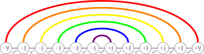
In the strong inhomogeneity limit $h\gg 1$, the application of the strong disorder renormalization group algorithm leads to a valence bond state built from singlets between the sites $m$ and $-m$, for $m=\frac{1}{2},\dots,L-\frac{1}{2}$ (in the XX version of the hamiltonian). Thus, the ground state resembles a rainbow like the one schematically represented in Fig. 2, where the colours of the bonds are associated to the energy required to break them, which is proportional to $e^{-2mh}$. The entanglement entropy between the left and right halves on this state is $S_{A}=L\log 2$, which corresponds to the highest value reachable for a subsystem containing $L$ qubits. In the limit $h\to\infty$ the rainbow state becomes the exact ground state of the hamiltonian (28), but several of its properties persist for all values of $h$. In particular, the entanglement entropy grows linearly with $L$ with a slope which depends on $h$.

In the limit $h\ll 1$ of weak inhomogeneity, the low energy physics of the hamiltonian (28) is described by the following hamiltonian of two chiral fermions $\psi_{L}$ and $\psi_{R}$ [11]

$$H\simeq\textrm{i}Ja\int_{-aL}^{aL}dx\,e^{-\frac{h|x|}{a}}\left[\psi^{\dagger}_{R}\,\partial_{x}\psi_{R}-\psi^{\dagger}_{L}\,\partial_{x}\psi_{L}-\frac{h}{2a}{\rm sign}{(x)}\Big(\psi^{\dagger}_{R}\psi_{R}-\psi^{\dagger}_{L}\psi_{L}\Big)\right],$$ (29)

where $a$ is the lattice spacing, $x=ma$ is the position and the fields $\psi_{L,R}(x)$ are the slow varying modes of the fermion operator $c_{m}$ expanded around the Fermi momenta $\pm k_{F}$ (where $k_{F}=\pi/(2a)$ at half filling), namely

$$\frac{c_{n}}{\sqrt{a}}\,\simeq\,e^{\textrm{i}k_{F}x}\,\psi_{L}(x)+e^{-\textrm{i}k_{F}x}\,\psi_{R}(x)\,.$$ (30)

The continuum limit corresponds to the regime where $a\rightarrow 0$, $h\rightarrow 0$ and $L\rightarrow\infty$, with $h/a$ and $aL$ kept constant. This implies that the product $\lambda\equiv hL$ is independent on the lattice spacing. Several quantities depend on this combination. We find it convenient to rename $h/a\rightarrow h$ and $aL\rightarrow L$. Thus, $h$ and $L$ acquire the dimensions respectively of an inverse length and a length. In (29) the fields $\psi_{L}$ and $\psi_{R}$ are decoupled in the bulk but their coupling comes from the boundary conditions [11]

$$\psi_{R}(\pm L)=\mp\,\textrm{i}\,\psi_{L}(\pm L)\,,$$ (31)

which are imposed at the endpoints of the segment.

4 Entanglement entropies for inhomogeneous fermionic systems

The powerful techniques of CFT in curved backgrounds have been successfully applied to study entanglement entropies of some configurations in some inhomogeneous fermionic systems such as the gas of free fermions trapped by the harmonic potential [6] and the rainbow model [10, 11, 13]. The conclusion of these works is that the long distance behavior of these models can be described by a massless Dirac fermion in a curved spacetime whose metric encodes the inhomogeneity parameters. The analytic expressions obtained for the entanglement entropies agree with high accuracy with the corresponding numerical results obtained through standard techniques.

The field theory we need to consider is a free massless Dirac fermion on the strip $\mathbb{S}$. Its two dimensional euclidean action reads

$$S=\int_{\mathbb{S}}\frac{dzd\bar{z}}{2\pi}\;e^{\sigma(x)}\left[\psi^{\dagger}_{R}\stackrel{{\scriptstyle\leftrightarrow}}{{\partial_{\bar{z}}}}\psi_{R}+\psi^{\dagger}_{L}\stackrel{{\scriptstyle\leftrightarrow}}{{\partial_{z}}}\psi_{L}\right],$$ (32)

where the background metric is given by

$$ds^{2}=e^{2\sigma(x)}dzd\bar{z}\,,$$ (33)

which is Weyl equivalent to the flat metric, with the Weyl factor $e^{\sigma(x)}$ depending only on the spatial variable. We remark that in the analysis of [6, 10] the worldsheet is the whole strip $\mathbb{S}$, while the worldsheet introduced in §2 is the strip where infinitesimal disks centered at the entangling points have been removed.

Since the Weyl factor does not depend on the Euclidean time $t\equiv t_{\textrm{\tiny E}}$, the metric (33) has a timelike Killing vector which guarantees that the corresponding Dirac hamiltonian derived from (32) is conserved. The complex coordinate $z$ in (33) is given in terms of coordinates $(x,t)$ as follows

$$z=\tilde{x}+\textrm{i}\,t\,,\qquad\tilde{x}=\int_{0}^{x}e^{-\sigma(y)}\,dy\,,$$ (34)

where $\tilde{x}$ is such that $\tilde{x}^{\prime}(x)=e^{-\sigma(x)}$. The scalar curvature of the metric (33) is given by

$${\cal R}=-\,2\,e^{-2\sigma(\tilde{x})}\,\partial_{\tilde{x}}^{2}\sigma(\tilde{x})=-\,2\big[\big(\partial_{x}\sigma(x)\big)^{2}+\partial_{x}^{2}\sigma(x)\big]\,,$$ (35)

where (34) has been employed in the last step. We consider background metrics that are symmetric with respect to the center $x=0$ of the segment, namely $\sigma(-x)=\sigma(x)$. In these cases we have

$$\tilde{x}\in(-\tilde{L},\tilde{L})\,,\;\;\qquad\;\;\tilde{L}\equiv\int_{0}^{L}e^{-\sigma(y)}\,dy\,.$$ (36)

For the Fermi gas trapped in a harmonic potential, the Weyl factor is the local Fermi velocity $e^{\sigma(x)}=v_{F}(x)$, which is given by [6]

$$e^{\sigma(x)}=\sqrt{L^{2}-x^{2}}\qquad\Longrightarrow\qquad\tilde{x}=\arcsin\frac{x}{L}\,,\qquad\tilde{L}=\frac{\pi}{2}\,.$$ (37)

The scalar curvature of this background is ${\cal R}=2/[L^{2}(\cos\tilde{x})^{4}]$. For an arbitrary external potential $V(x)$, one has $e^{\sigma(x)}=v_{F}(x)=\sqrt{2(\mu-V(x))}$, where $\mu$ is the number of particles in the gas.

In the rainbow model, the Weyl factor encodes the local hopping amplitudes decreasing exponentially from the center towards the edges of the segment [10]. It reads

$$e^{\sigma(x)}=e^{-h|x|}\qquad\Longrightarrow\qquad\tilde{x}={\rm sign}(x)\frac{e^{h|x|}-1}{h}\,,\qquad\tilde{L}=\frac{e^{hL}-1}{h}\,,$$ (38)

where $h\geqslant 0$. The scalar curvature of this background is ${\cal R}=-2h^{2}+4h\delta(\tilde{x})$, namely it is constant and negative everywhere except for a singularity at the origin. These inhomogeneous models become uniform by taking a specific limit.

The entanglement entropies for an interval $A=(x_{0},L)$ adjacent to the boundary of the segment $(-L,L)$ in these inhomogeneous fermionic systems have been computed by employing the twist field method [6]. The result is

$${\rm Tr}\,\rho_{A}^{n}=\eta^{\Delta_{n}}\langle{\cal T}_{n}(x_{0},0)\rangle_{\textrm{\tiny curved}}\,,$$ (39)

where ${\cal T}_{n}(x_{0},0)$ is a twist field at the entangling point $(x,t_{\textrm{\tiny E}})=(x_{0},0)$, whose dimension $\Delta_{n}$ is given by (with $c=1$ for a free fermion)

$$\Delta_{n}=\frac{1}{12}\left(n-\frac{1}{n}\right),$$ (40)

and $\eta$ is a UV cutoff, whose relation with the cutoff $\epsilon$ introduced in §2 is discussed below.

The expectation value (39) is computed with the action (32) that contains the Weyl factor $e^{\sigma}$. A Weyl rescaling transforms the metric (33) into the flat metric $dzd\bar{z}$. Under this transformation the twist operator transforms as

$${\cal T}_{n}(x_{0},0)\,\rightarrow\,\big(\tilde{x}^{\prime}(x_{0})\big)^{\Delta_{n}}\,{\cal T}_{n}(\tilde{x}_{0},0)\,=\,e^{-\Delta_{n}\sigma(x_{0})}\,{\cal T}_{n}(\tilde{x}_{0},0)\,.$$ (41)

Thus (39) becomes

$${\rm Tr}\,\rho_{A}^{n}=\eta^{\Delta_{n}}e^{-\Delta_{n}\sigma(x_{0})}\langle{\cal T}_{n}(\tilde{x}_{0},0)\rangle_{\textrm{\tiny flat}}\,,$$ (42)

where $\tilde{x}_{0}\equiv\tilde{x}(x_{0})$. The correlator $\langle{\cal T}_{n}(\tilde{x}_{0},0)\rangle_{\textrm{\tiny flat}}$ is computed on the strip $(-\tilde{L},\tilde{L})\times\mathbb{R}$ with flat background, which can be mapped into the flat upper half plane (UHP) through the transformation $z\rightarrow g(z)=e^{\textrm{i}\pi(\tilde{L}-z)/(2\tilde{L})}$; therefore we have

$${\rm Tr}\,\rho_{A}^{n}=\eta^{\Delta_{n}}e^{-\Delta_{n}\sigma(x_{0})}\left|\frac{dg}{d\tilde{x}}\right|^{\Delta_{n}}_{\tilde{x}=\tilde{x}_{0}}\langle{\cal T}_{n}(g(\tilde{x}_{0}),\bar{g}(\tilde{x}_{0}))\rangle_{\textrm{\tiny uhp}}\,.$$ (43)

By employing the following correlator in the upper half plane

$$\langle{\cal T}_{n}(g(\tilde{x}),\bar{g}(\tilde{x}))\rangle_{\textrm{\tiny uhp}}=({\rm Im}\,g(\tilde{x}))^{-\Delta_{n}}=\left(\sin\frac{\pi(\tilde{L}-\tilde{x})}{2\tilde{L}}\right)^{-\Delta_{n}},$$ (44)

one obtains

$${\rm Tr}\,\rho_{A}^{n}=\left[\,e^{\sigma(x_{0})}\,\frac{2\tilde{L}}{\pi\eta}\,\sin\frac{\pi(\tilde{L}-\tilde{x}_{0})}{2\tilde{L}}\,\right]^{-\Delta_{n}}.$$ (45)

This gives the following expression for the entanglement entropies

$$S^{(n)}_{A}=\frac{1}{12}\left(1+\frac{1}{n}\right)\log\left[\,e^{\sigma(x_{0})}\,\frac{2\tilde{L}}{\pi\eta}\,\sin\frac{\pi(\tilde{L}-\tilde{x}_{0})}{2\tilde{L}}\,\right],$$ (46)

which coincides with the formula of the entanglement entropies of an interval $(\tilde{x}_{0},\tilde{L})$ in the segment $(-\tilde{L},\tilde{L})$ for the homogenous models, except for the additional constant term due to the factor $e^{\sigma(x_{0})}$ inside the argument of the logarithm.

As for the Fermi gas trapped in a harmonic potential, where the density depends on the position, in [6] it has been explained that a further spatial dependence must be introduced in the UV cutoff as $\eta\to\eta(x)=\eta_{0}/k_{\textrm{\tiny F}}(x)$, being $k_{\textrm{\tiny F}}(x)=\sqrt{L^{2}-x_{0}^{2}}$ the Fermi momentum. By employing this important observation and (37) in (46), one finds [6]

$$S^{(n)}_{A}=\frac{1}{12}\left(1+\frac{1}{n}\right)\log\left[\frac{L^{2}}{\eta_{0}}\left(1-\frac{x^{2}_{0}}{L^{2}}\right)^{3/2}\,\right].$$ (47)

In the rainbow model, where $k_{\textrm{\tiny F}}=\pi/2$ and the inhomogeneity is due to the spatial dependence of the couplings, there is no need to introduce a spatial dependence for the UV cutoff $\eta$; therefore, by using (38) in (46), one obtains [13]

$$S^{(n)}_{A}=\frac{1}{12}\left(1+\frac{1}{n}\right)\log\left[\,e^{-h|x_{0}|}\frac{2(e^{hL}-1)}{\pi h\,\eta}\,\cos\left(\frac{\pi}{2}\frac{e^{h|x_{0}|}-1}{e^{hL}-1}\right)\right].$$ (48)

In [6] and [13] the entanglement entropies of free fermions trapped by the harmonic potential and of the rainbow chain respectively have been studied also numerically through standard techniques for free fermions on the lattice. Complete agreement has been obtained between with the analytic expressions reported in (47) and (48).

5 Entanglement hamiltonian for inhomogeneous systems

In this section we employ the results of [24] reviewed in §2 to study the entanglement hamiltonian and the corresponding entanglement spectrum for the interval $A=(x_{0},L)$ in the segment $(-L,L)$ in the inhomogeneous systems described in §3 and §4.

The analysis of [24] has been carried out in flat spacetimes, where $ds^{2}=dzd\bar{z}$. In curved spacetimes with background metric $ds^{2}=e^{2\sigma}dzd\bar{z}$, the regularisation procedure and the conformal mappings described in §2 can be repeated, finding that

$${\rm Tr}\,\rho^{n}_{A}\,=\,e^{-2\pi nK_{A}}\,=\,\frac{\mathcal{Z}_{n\textrm{\tiny-annulus, curved}}}{\mathcal{Z}_{\textrm{\tiny annulus, curved}}^{n}}\,,$$ (49)

which is different from (6) because the curved background metric occurs in the annular partition functions.

In the appendix A we employ the characteristic property of Liouville theory [37, 38] to argue that $\mathcal{Z}_{\textrm{\tiny annulus, curved}}=\Omega\,\mathcal{Z}_{\textrm{\tiny annulus, flat}}$ and $\mathcal{Z}_{n\textrm{\tiny-annulus, curved}}=\Omega^{n}\mathcal{Z}_{n\textrm{\tiny-annulus, flat}}$, where $\Omega$ is a positive factor. Focussing on the inhomogeneous systems whose background is described by (33), this observation implies that ${\rm Tr}\rho_{A}^{n}$ is given by the same expression found for the flat geometry in terms of the coordinates $(\tilde{x},t)$ (see (34)). This result can be obtained if the same construction holds also for the entanglement hamiltonian. In particular, from (5) we can write the entanglement hamiltonian $K_{A}$ in the inhomogeneous systems characterised by (33) as follows

$$K_{A}=\int_{\tilde{A}}\frac{T_{00}(\tilde{x})}{\tilde{f}^{\prime}(\tilde{x})}\;d\tilde{x}\,,$$ (50)

where the integration domain is $\tilde{A}\equiv(\tilde{x}_{0},\tilde{L})$, which can be found from (34) and (36). In (50) we have denoted by $\tilde{f}(x)$ the function obtained from $f(x)$ by replacing all the parameters with the corresponding tilded ones. By employing the transformation law $T_{00}(\tilde{x})=\tilde{x}^{\prime}(x)^{-2}\,T_{00}(x)$ for the component of the energy-momentum tensor (the schwarzian derivative term can be neglected in this analysis, as argued in [24]), the entanglement hamiltonian (50) can be expressed in terms of the original spatial variable $x$ as follows

$$K_{A}=\int_{A}\beta_{A}(x)\,T_{00}(x)\,dx\,,$$ (51)

where $A=(x_{0},L)$ and the weight function $\beta_{A}(x)$ is given by

$$\beta_{A}(x)\,=\,\frac{1}{\tilde{x}^{\prime}(x)\,\tilde{f}^{\prime}(\tilde{x}(x))}\,,$$ (52)

which can be also written as $1/\beta_{A}(x)=\tfrac{d\tilde{f}(\tilde{x}(x))}{dx}$. Since from (34) we have $\tilde{x}^{\prime}(x)=e^{-\sigma(x)}$, the positivity of $\beta_{A}(x)$ comes from the fact that $f^{\prime}(x)$ is positive (see (21)).

The expansion of $f^{\prime}(x)$ as $x\rightarrow x_{0}^{+}$ for the functions that we are considering is given by $f^{\prime}(x)=(x-x_{0})^{-1}+f_{0}+O(x-x_{0})$. As for (52) in this limit, we find that

$$\beta_{A}(x)\,=\,(x-x_{0})-\left(\tilde{x}^{\prime}(x_{0})\,\tilde{f}_{0}+\frac{\tilde{x}^{\prime\prime}(x_{0})}{2\,\tilde{x}^{\prime}(x_{0})}\right)(x-x_{0})^{2}+\dots\,,$$ (53)

where $\tilde{f}_{0}$ is the coefficient occurring in the expansion $\tilde{f}^{\prime}(x)=(x-x_{0})^{-1}+\tilde{f}_{0}+O(x-x_{0})$ as $x\to x_{0}^{+}$ and the dots denote subleading terms. The leading term in (53) corresponds to the characteristic behaviour described by the Bisognano-Wichmann theorem and it does not depend on the features of the underlying model, occurring instead in the subleading term. By using that $\tilde{x}^{\prime}(x)=e^{-\sigma(x)}$, which implies $\tilde{x}^{\prime\prime}(x)/\tilde{x}^{\prime}(x)=-\,\sigma^{\prime}(x)$, we obtain that the coefficient of $(x-x_{0})^{2}$ in (53) simplifies to $\sigma^{\prime}(x_{0})/2-e^{-\sigma(x_{0})}\tilde{f}_{0}$.

For the configuration given by the interval $A=(x_{0},L)$ in the segment $(-L,L)$, the conformal map to consider is (20). The weight function (52) for the entanglement hamiltonian can be written explicitly by employing (21), finding

$$\beta_{A}(x)\,=\,\frac{2\tilde{L}}{\pi}\;\frac{\sin(\pi\tilde{x}(x)/(2\tilde{L}))-\sin(\pi\tilde{x}_{0}/(2\tilde{L}))}{\cos(\pi\tilde{x}_{0}/(2\tilde{L}))\,\tilde{x}^{\prime}(x)}\,,$$ (54)

where $\tilde{x}_{0}=\tilde{x}(x_{0})$. We remark that $\beta_{A}(x)$ does not contain the UV cutoff.

The expansion (54) as $x\to x_{0}^{+}$ is (53), where the coefficient of $(x-x_{0})^{2}$ can be written explicitly by using (38) and that $\tilde{f}_{0}=\tfrac{\pi}{4\tilde{L}}\tan(\tfrac{\pi\tilde{x}_{0}}{2\tilde{L}})$ (see (22)).

The above discussion naturally leads to consider the width of the flat annulus in terms of the tilded quantities. From (23), it reads

$$\widetilde{W}_{A}=\log\bigg[\frac{4\tilde{L}}{\pi{\tilde{\epsilon}}}\sin\bigg(\frac{\pi\tilde{\ell}}{2\tilde{L}}\bigg)\bigg]+O(\tilde{\epsilon})\,,\;\qquad\;\tilde{\ell}=\tilde{L}-\tilde{x}_{0}\,.$$ (55)

The UV cutoff $\tilde{\epsilon}$ in this expression plays a crucial role in our analysis. It can be written in terms of the physical UV cutoff $\epsilon$ by using that the endpoints of the interval $\tilde{A}_{\tilde{\epsilon}}=(\tilde{x}_{0}+\tilde{\epsilon},\tilde{L})$ are related to the corresponding endpoints of $A_{\epsilon}=(x_{0}+\epsilon,L)$. In particular, from the first endpoints of these two intervals, we have

$$\tilde{x}(x_{0}+\epsilon)=\tilde{x}_{0}+\tilde{\epsilon}+O(\epsilon^{2})\qquad\Longrightarrow\qquad\tilde{\epsilon}=\,e^{-\sigma(x_{0})}\,\epsilon\,,$$ (56)

where $\tilde{x}^{\prime}(x_{0})=e^{-\sigma(x_{0})}$ has been employed. We remark that the inhomogeneity in some models (e.g. the trapping potentials in [6]) requires to introduce a UV cutoff $\epsilon$ which depends on $x_{0}$. This dependence cannot be captured through our CFT analysis.

The entanglement entropies for the interval $A=(x_{0},L)$ in the segment $(-L,L)$ in the inhomogeneous models can be easily written from (7), (55) and (56), finding

$$S^{(n)}_{A}=\frac{c}{12}\left(1+\frac{1}{n}\right)\widetilde{W}_{A}\,=\,\frac{c}{12}\left(1+\frac{1}{n}\right)\log\bigg[e^{\sigma(x_{0})}\;\frac{4\tilde{L}}{\pi{\epsilon}}\sin\bigg(\frac{\pi\tilde{\ell}}{2\tilde{L}}\bigg)\bigg]\,,$$ (57)

up to a constant term. This result coincides with the expression (46) obtained through the twist field method, once the relation $\epsilon=2\eta$ between the UV parameters is imposed. Thus, the method of [24] allows to recover the results of [6, 13], once the possible spatial dependence in the UV cutoff is properly taken into account [6], as mentioned in §4.

The above analysis gives access also to the entanglement spectrum. Combining the expressions (10) and (11) with (55) and (56), for the eigenvalues of the reduced density matrix in the inhomogeneous models we find

$$-\log\lambda_{j} = -\left(\Delta_{j}-\frac{c}{24}\,\right)\log(e^{-2\pi^{2}/\widetilde{W}_{A}})+\log\widetilde{\mathcal{Z}}_{\textrm{\tiny annulus}}$$ (58)

$$= \frac{c}{12}\,\widetilde{W}_{A}+\log\big(\langle a|0\rangle\langle 0|b\rangle\big)+\left(\Delta_{j}-\frac{c}{24}\right)\frac{2\pi^{2}}{\widetilde{W}_{A}}+O(\epsilon^{r})\,,$$ (59)

where (56) has been employed in the last step also to evaluate the neglected terms. By comparing (57) and (59), it is straightforward to realise that $-\log\lambda_{j}=S_{A}/2$ for any $j$ at leading order also in the inhomogeneous case.

The maximum eigenvalue corresponds to $\Delta_{j}=0$; therefore we have

$$-\log\lambda_{\textrm{\tiny max}}\,=\,\frac{c}{12}\,\widetilde{W}_{A}+\log\big(\langle a|0\rangle\langle 0|b\rangle\big)-\frac{\pi^{2}c}{12\,\widetilde{W}_{A}}+O(\epsilon^{r})\,.$$ (60)

The gaps in the entanglement spectrum are also interesting quantities to consider and they can be easily obtained from (58), finding $\log\lambda_{j}-\log\lambda_{k}=2\pi^{2}(\Delta_{k}-\Delta_{j})/\widetilde{W}_{A}$. As for the gaps with respect to the maximum eigenvalue, they read

$$\mathcal{E}_{k}=\log\lambda_{\textrm{\tiny max}}-\log\lambda_{k}=\frac{2\pi^{2}\Delta_{k}}{\widetilde{W}_{A}}\,.$$ (61)

From (57) and (61), also for these inhomogeneous cases we obtain (see (15))

$$S^{(n)}_{A}\,\mathcal{E}_{k}\,=\,\frac{\pi^{2}}{6}\left(1+\frac{1}{n}\,\right)\Delta_{k}+\dots\,,$$ (62)

where the dots correspond to terms which vanish as $\epsilon\to 0$. Let us remark that the r.h.s. of (62) is independent of the inhomogeneity parameters.

6 An entanglement contour for inhomogeneous systems

The contour for the entanglement entropies in lattice models has been introduced in §1. Explicit constructions has been proposed in [27] for free fermions and in [29] for harmonic lattices (see also [26, 28]).

In the continuum limit, the conditions (3), that are necessary but not sufficient to define a proper contour function for the entanglement entropies, become respectively

$$S_{A}^{(n)}=\int_{A_{\epsilon}}s_{A}^{(n)}(x)\,dx\,,\;\;\qquad\;\;s_{A}^{(n)}(x)\geqslant 0\,.$$ (63)

Although these conditions (or their counterparts (3) in the lattice) does not allow to find the function $s_{A}^{(n)}(x)$ in a unique way, in [29] it has been observed that the analysis of [24] provides a natural candidate for the contour function for the entanglement entropies in CFT, restricted to the class of configurations considered in [24], which includes the one of our interest. In the following, by employing the results of §5, we adapt the observation made in [29] for the homogeneous models to the inhomogeneous systems discussed above.

Considering the configuration we are interested in, namely the subsystem $A=(x_{0},L)$ in the segment $(-L,L)$, the integration domain in (63) is the interval $A_{\epsilon}=(x_{0}+\epsilon,L)$.

In order to construct the contour function for the entanglement entropies of this configuration in inhomogeneous models, from (23), we notice that the expression (55) can be written as

$$\widetilde{W}_{A}=\int_{\tilde{A}_{\tilde{\epsilon}}}\tilde{f}^{\prime}(\tilde{x})\,d\tilde{x}=\tilde{f}(\tilde{L})-\tilde{f}(\tilde{x}_{0}+\tilde{\epsilon})\,.$$ (64)

By employing this observation in (57), we find for the entanglement entropies that

$$S_{A}^{(n)}=\frac{c}{12}\left(1+\frac{1}{n}\right)\int_{A_{\epsilon}}\tilde{f}^{\prime}(\tilde{x}(x))\,\tilde{x}^{\prime}(x)\,dx\,,$$ (65)

up to a additive constant term. Then, by comparing (63) and (65), we are naturally lead to the following candidate for the contour function of the entanglement entropies

$$s_{A}^{(n)}(x)=\frac{c}{12}\left(1+\frac{1}{n}\right){\cal S}_{A}(x)+\frac{C_{n}}{\ell}\,,$$ (66)

where the function ${\cal S}_{A}(x)$ is defined as follows

$${\cal S}_{A}(x)=\tilde{x}^{\prime}(x)\,\tilde{f}^{\prime}(\tilde{x}(x))\,,$$ (67)

and $C_{n}$ is the non universal constant term in (7). We find it worth remarking that the contour function (66) does not depend on the UV cutoff, which plays a crucial role in the determination of the spatial dependence of the entanglement entropies in the specific model, as mentioned in §4.

Let us consider the behaviour of the contour function (66) as $x\to x_{0}^{+}$. This can be easily done by exploiting the similar analysis made for the weight function (52), whose result is (53), which can be written also in a form involving the Weyl factor reported in the text below (53). From the latter observation we find that

$$\mathcal{S}_{A}(x)=\frac{1}{x-x_{0}}+e^{-\sigma(x_{0})}\tilde{f}_{0}-\frac{\sigma^{\prime}(x_{0})}{2}+O\big((x-x_{0})\big)\,,$$ (68)

where $\tilde{f}_{0}$ has been introduced in the text below (53). The leading term in (68) is responsible of the logarithmic divergence in the entanglement entropies as $\epsilon\to 0$. Thus, the contour function that we have constructed can quantify the expectation that the entanglement between two regions is mainly due to the parts of the complementary regions close to the entangling point separating $A$ and $B$.

It is interesting to mention that, by comparing (52) and (67), one finds the following relation

$$\beta_{A}(x)\,{\cal S}_{A}(x)=1\,,$$ (69)

which can be expressed also in terms of the contour function for the entanglement entropies (66). Indeed, by introducing the proper factors from (1), (51) and (66), we have that (69) leads to

$$\big[2\pi\beta_{A}(x)\big]s^{(n)}_{A}(x)=\frac{\pi}{6}\left(1+\frac{1}{n}\,\right)c\,+\dots\,,$$ (70)

where the dots corresponds to infinitesimal terms as $\epsilon\to 0$. The relation (70) exhibits an intriguing similarity with (62), with the crucial difference that the quantities involved in the l.h.s. of (70) depend on the position $x\in A$.

7 Numerical results for the rainbow chain

The analytic expressions discussed in §5 and §6 hold for a generic CFT in the static background given by (33).

In this section we focus on the rainbow model. Considering rainbow chains defined by (28), we present numerical confirmation of the analytic expressions of §5 and §6 for this model. In particular, for the configuration given by a block $A$ adjacent to the boundary of a segment, we compute the entanglement hamiltonian, the entanglement spectrum and a contour for the entanglement entropies.

7.1 Entanglement hamiltonian

In order to estimate the entanglement hamiltonian for a block of our system, we have developed an ab initio numerical procedure similar to the one based on machine learning techniques described in [33]. A different approach has been proposed in [39].

The starting point of our numerical procedure is the following ansatz for the entanglement hamiltonian

$$H_{A}(\boldsymbol{\beta})\,=\,-\,\frac{1}{2}\sum_{i\,\in\,A}\beta_{i}\,d^{\dagger}_{i}d_{i+1}+\textrm{h.c.}\,,$$ (71)

where $\boldsymbol{\beta}=\{\beta_{i}\,,i\in A\}$ is the vector whose elements are the couplings of the entanglement hamiltonian. We remark that the ansatz (71) does not capture the complete entanglement hamiltonian of the underlying lattice model. Indeed, considering the detailed results obtained in [23, 25] for a single block in a homogenous chain of free fermions on the infinite line, in the entanglement hamiltonian non vanishing couplings occur also between sites that are not nearest neighbours. Nonetheless, these couplings are expected to be very small, therefore we are allowed to neglect them as first approximation.

In order to impose that the elements of the vector $\boldsymbol{\beta}$ provide a density matrix $\rho_{A}(\boldsymbol{\beta})\equiv e^{-H_{A}(\boldsymbol{\beta})}$ approximating the reduced density matrix $\rho_{A}$ for the subsystem $A$, we exploit the Wick’s theorem, which ensures that $\rho_{A}$ is characterised by the correlation matrix $C_{ij}\equiv\langle c^{\dagger}_{i}c_{j}\rangle$ restricted to the block $A$, i.e. with $i$, $j\in A$. Thus, given a choice of $\boldsymbol{\beta}$, let us introduce

$$C_{ij}(\boldsymbol{\beta})\equiv{\rm Tr}\big(\rho_{A}(\boldsymbol{\beta})\,d^{\dagger}_{i}d_{j}\big)\,,\;\;\qquad\;\;i,j\,\in\,A\,,$$ (72)

with $\rho_{A}(\boldsymbol{\beta})$ defined through (71), and also the following error function

$$E(\boldsymbol{\beta})\equiv\sum_{i,j\,\in\,A}\big[C_{ij}-C_{ij}(\boldsymbol{\beta})\big]^{2}\,.$$ (73)

The numerical values for the elements of $\boldsymbol{\beta}$ are obtained by minimising this error function through standard optimization techniques (Powell method) [40]. The optimization procedure begins with a homogeneous seed and then seeks a value of $\boldsymbol{\beta}$ which fits the exact correlation matrix within a certain tolerance, which is fixed to $10^{-6}$ in the worst case. Our algorithm was able to find a solution for all the cases that we have explored.

In the continuum limit, by comparing (1) with (71) , we expect that $H_{A}(\boldsymbol{\beta})\to 2\pi K_{A}$, where $K_{A}$ is the entanglement hamiltonian (51). For a Dirac fermion, the component $T_{00}(x)$ of the energy-momentum tensor is given by

$$T_{00}(x)\,=\,\textrm{i}\left(\psi^{\dagger}_{R}(x)\partial_{x}\psi_{R}(x)-\psi^{\dagger}_{L}(x)\partial_{x}\psi_{L}(x)\right).$$ (74)

Thus, for the couplings $\beta_{i}$ in (71) we expect that $\beta_{i}\to 2\pi\beta_{A}(x)$ in the continuum limit.

The weight function $\beta_{A}(x)$ to adopt in (51) for the rainbow model can be constructed by specifying the general expression (54) for the map $\tilde{x}(x)$ characterising the rainbow model, given in (38). This leads to the following expression

$$\beta_{A}(x)\;=\;\frac{2(e^{\lambda}-1)L}{\pi\lambda}\;\,\frac{\sin\big(\tfrac{\pi}{2}\,\tfrac{(e^{\lambda|x/L|}-1)\,\textrm{sign}(x/L)}{e^{\lambda}-1}\big)-\sin\big(\tfrac{\pi}{2}\,\tfrac{(e^{\lambda|x_{0}/L|}-1)\,\textrm{sign}(x_{0}/L)}{e^{\lambda}-1}\big)}{e^{\lambda|x/L|}\,\cos\big(\tfrac{\pi}{2}\,\tfrac{(e^{\lambda|x_{0}/L|}-1)\,\textrm{sign}(x_{0}/L)}{e^{\lambda}-1}\big)}\,.$$ (75)

From this formula it is straightforward to observe that $\beta_{A}(x)/L$ is a function of $x/L$, where $\lambda=hL$ and $x_{0}/L$ enter as the parameters characterising the subsystem $A$. In the homogeneous case, namely for $h=0$, we have that (75) reduces to (21), as expected. Also the expansion (53) of $\beta_{A}(x)$ for $x\to x_{0}^{+}$ can be specified for the rainbow model, but we do not report the resulting expression. Let us stress that the features of the model occur in the subleading $O((x-x_{0})^{2})$ term of (53).

We find it more instructive first to discuss (75) for some interesting special regimes.

Figure 3: Couplings $\beta_{i}/L$ in the entanglement hamiltonian (71) corresponding to the right half $A=(0,L)$, i.e. for $x_{0}=0$, of various rainbow chains, obtained numerically as discussed in §7.1. The data points agree with the analytic expression of $2\pi\beta_{A}(x)/L$ in (76), which is a function of $x/L$ parameterised by $\lambda=hL$. The dashed-dotted straight line has slope $2\pi$ and highlights the behaviour inherited from the Bisognano-Wichmann theorem near the entangling point $x_{0}=0$. When $\lambda\gg 1$ a plateau occurs which provides the thermofield double interpretation for the ground state of the rainbow chain in the strong coupling regime (see (78)).

When the block $A$ is half of the rainbow chain, the weight function in the entanglement hamiltonian can be obtained by setting $x_{0}=0$ in (75). The result reads

$$\beta_{A}(x)\,\equiv\,\frac{2L}{\pi}\;\frac{e^{\lambda}-1}{\lambda}\;e^{-\lambda x/L}\;\sin\bigg(\frac{\pi}{2}\;\frac{e^{\lambda x/L}-1}{e^{\lambda}-1}\bigg)\,,$$ (76)

with $x\in(0,L)$, which is manifestly positive. Taking $\lambda\gg 1$ in (76), we find

$$\beta_{A}(x)\,=\,\frac{1}{h}\big(1-e^{-hx}\big)+\dots\,,$$ (77)

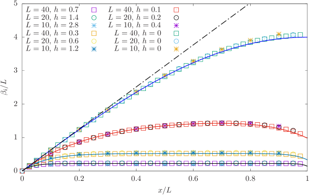
where the dots denote subleading terms. The expansion (77) captures the main features of this regime; indeed, $\beta_{A}(x)\simeq x$ for $x\ll 1/h$ and $\beta_{A}(x)\simeq 1/h$ for $x\gg 1/h$; namely $\beta_{A}(x)$ is linear near to the entangling point and becomes flat for a large part of the remaining interval.

In Fig. 3 we show the numerical values of the coefficients $\beta_{i}/L$ for the right half (i.e. $x_{0}=0$) of various rainbow chains as a function of $x/L$ (with $i=x$), along with the theoretical prediction $2\pi\beta_{A}(x)/L$ in the continuum limit given by (76), which is parameterised by the combination $\lambda=hL$. An excellent agreement is observed between the numerical data and the CFT formula along the entire subsystem $A$. For $x\simeq x_{0}^{+}$, notice the peculiar behaviour of the Bisognano-Wichmann theorem, which corresponds to the dashed and dotted line in Fig. 3, as expected from (53).

In the homogeneous case, i.e. for $h=0$, the data for $\beta_{i}/L$ in Fig. 3 follow the CFT curve (21). As $\lambda$ increases, the $\beta_{i}/L$ develops a plateau at a height $2\pi/\lambda$, in agreement with the prediction (77).

Figure 4: Correlation matrix for the rainbow state compared to the thermofield double approximation. For different rainbow systems with $L=40$, we show $|\langle c^{\dagger}_{i}c_{j}\rangle|$, with $j=20$. The points having $i=1,\dots,40$ have been computed using a thermal density matrix of a hamiltonian with uniform couplings and temperature (79). The continuos lines correspond to the exact correlations in the rainbow ground state, which have been evaluated for the entire chain. Precise agreement is found within the block $A$ between the two different computations of the correlator. A peak occurs also at the site $i=-20$, which is entangled with the site $i=20$ because of a long distance bond.

An interesting consequence of (77) is that we can approximate the reduced density matrix for $\lambda\gg 1$ as follows

$$\rho_{A}\simeq{\rm exp}\left(-\,\frac{2\pi}{h}\int_{A}T_{00}(x)\,dx\right),$$ (78)

which is the thermal density matrix of a CFT with $c=1$ and an effective temperature given by [11]

$$T_{R}=\frac{h}{2\pi}\,.$$ (79)

This result is consistent with the entanglement entropy (48) in this regime, which becomes $S_{A}\simeq hL/6$ for $n=1$, namely the thermal entropy of a CFT with $c=1$ at finite temperature (79).

The latter observation about the entanglement entropy led to the interpretation of the ground state of the rainbow model as a thermofield double [11], that is a pure state defined on the tensor product $\mathcal{H}_{l}\otimes\mathcal{H}_{r}$ of two copies of the same Hilbert space associated to a CFT and whose Schmidt decomposition is given by

$$|\psi\rangle=\sum_{n}e^{-\frac{1}{2}\beta_{R}E_{n}}\,|n\rangle_{l}\,|n\rangle_{r}\,,\;\;\qquad\;\;\beta_{R}=\frac{1}{T_{R}}\,,$$ (80)

where $|n\rangle_{l}$ and $|n\rangle_{r}$ are the eigenstates of a CFT hamiltonian corresponding to the energy level $E_{n}$ for the left and right blocks of the system. Tracing out either the left or the right half of the system gives $\sum_{n}e^{-\beta_{R}E_{n}}|n\rangle\langle n|$, which is the thermal density matrix of a single CFT with inverse temperature $\beta_{R}$.

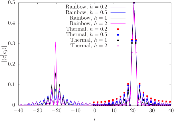
A consequence of the thermofield double structure of the ground state of the rainbow chain is that the expectation values of operators belonging to the same half chain can be obtained as averages on half chain at finite temperature $T_{R}$ given by (79). Considering, for instance, the correlator $\langle c^{\dagger}_{i}c_{j}\rangle$, in Fig. 4 we show the values of $|\langle c^{\dagger}_{i}c_{j}\rangle|$ for a chain with $2L=80$ sites, $j=20$ and $i=1,2,\dots,40$. Taking the right half chain as subsystem, for $i\geqslant 1$ this correlator can be computed also as a correlator of a uniform chain made by $40$ sites at finite temperature $T_{R}$. An excellent agreement is observed between these two ways to compute this correlator.

Figure 5: Couplings $\beta_{i}/L$ in the entanglement hamiltonian (71) for the block $A=(x_{0},L)$ with $x_{0}=-L/2$ in various rainbow chains, obtained numerically as discussed in §7.1. The continuos solid lines correspond to the analytic prediction for $2\pi\beta_{A}(x)/L$ given by (75) in terms of $x/L$. The values of $L$ and $h$ have been chosen in order to highlight the collapse of the numerical data having the same $\lambda=hL$. The decay from $x=0$ outwards is approximately exponential. The vertical dashed line, marks the boundary between the active and inactive regions. Inset: zoom for $x\sim x_{0}^{+}$, which emphasizes the Bisognano-Wichmann behavior (dashed straight line with slope $2\pi$) near the entangling point.

Finally, let us consider blocks $A=(x_{0},L)$ having $x_{0}\neq 0$. The general expression for the weight function $\beta_{A}(x)$ in the entanglement hamiltonian (51) is given by (75), which is a positive function for $x\in A$, as discussed below (52). Taking the limit $\lambda\gg 1$ of (75) with fixed $x/L$, we find

$$\beta_{A}(x)\,\simeq\,\frac{\textrm{sign}(x)-\textrm{sign}(x_{0})\,e^{-h(|x|-|x_{0}|)}}{h}\,,$$ (81)

where we have reported only the leading terms. When $x_{0}>0$ we get that $\beta_{A}(x)\simeq(1-e^{-h(x-x_{0})})/h$, which reduces to (77) for $x_{0}=0$, as expected. The qualitative behaviour of $\beta_{A}(x)$ for $x_{0}>0$ is very similar to the one observed for the $x_{0}=0$ case. Instead, when $x_{0}<0$ the expression (81) becomes

$$\beta_{A}(x)\,\simeq\,\left\{\begin{array}[]{ll}e^{h(|x_{0}|-|x|)}/h&-|x_{0}|<x<|x_{0}|\,,\\ \rule{0.0pt}{17.07182pt}1/h&|x_{0}|<x<L\,,\end{array}\right.$$ (82)

which displays qualitative different features; indeed an exponential behavior is observed in the region $|x|<|x_{0}|$ and the usual plateau $\beta_{A}(x)\simeq 1/h$ occurs for $x>|x_{0}|$.

An intuitive explanation of this behaviour is the following. The rainbow state in the strong coupling limit is composed of long-distance valence bonds symmetrically placed around the origin, between sites at $+x$ and $-x$ (see Fig. 2). Thus, in this limit it is natural to identify two regions of the interval $A=(x_{0},L)$, with $x_{0}<0$: an inactive zone $(-|x_{0}|,+|x_{0}|)$ containing bonds which do not leave the block, and an active zone $(|x_{0}|,L)$, which contains bonds linking the block $A$ to its complement $B$. The vertical dashed line in Fig. 5 separates these two regions in $A$. For any finite $h$, fluctuations in the active zone are higher than the ones in the inactive zone because of the broken bonds. Thus, in the limit of large $\lambda$, the coefficients of the entanglement hamiltonian present the usual plateau of height $1/h$ in the active zone, while in the inactive zone they present an exponential decay from the origin which is similar to the one occurring in the original Hamiltonian.

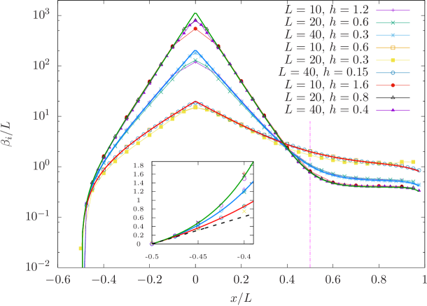
The fact that the couplings $\beta_{i}$ take very high values in the inactive zone (the peak is reached at the origin, where $\beta_{A}(0)\propto\exp(h|x_{0}|)$) inhibits fluctuations in that zone. Indeed, in Fig. 5 we can observe that our numerical technique to estimate $\beta_{i}$ makes larger errors near $x=0$. This happens because the high values of the couplings $\beta_{i}$ in the inactive region cause the elements of the correlation matrix to be rather insensitive to details on the $\beta_{i}$’s.

7.2 Entanglement spectrum

The reduced density matrix $\rho_{A}$ of a free fermion system decomposes into the product of single body density matrices [23]

$$\rho_{A}\,=\,e^{-\sum_{p}\varepsilon_{p}\,\hat{n}_{p}-r_{0}}\,,$$ (83)

where $\hat{n}_{p}$ are the occupation number operators, whose eigenvalues are either 0 or 1, and the corresponding $\varepsilon_{p}$ are called single body entanglement energies, which are related to the eigenvalues $\nu_{p}=\langle\hat{n}_{p}\rangle$ of the block correlation matrix $C_{ij}=\langle c^{\dagger}_{i}c_{j}\rangle$ with $i,j\in A$ as follows

$$\nu_{p}\,=\,\frac{1}{\exp(\varepsilon_{p})+1}\,.$$ (84)

The normalization condition ${\rm Tr}\rho_{A}=1$ for (83) provides the constant $r_{0}$. The eigenvalues of $\rho_{A}$ in (83) can be written as $\lambda_{j}\equiv e^{-E_{j}}\in(0,1)$, in terms of the entanglement energies $E_{j}$, which can be obtained as $E_{j}=\sum_{p}\varepsilon_{p}n_{p}+r_{0}$, where the index $j$ denotes the set $\{n_{p}\}$ of the occupation numbers providing $E_{j}$.

Figure 6: Single body entanglement energies for a rainbow systems with $L=100$. Left: Rainbow chain with $h=1.4$ fixed and different values of the block size $\ell$, from 20 up to 100. Right: Rainbow chain with different values of $h$ and the block $A$ made by half chain. An approximately linear behavior is observed in all cases, confirming the theoretical prediction given by (92) and (93).

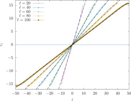
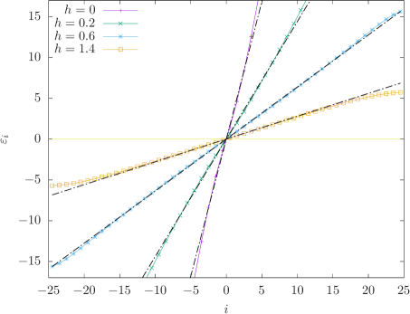
In Fig. 6 we show the single body entanglement energies $\varepsilon_{p}$ for a rainbow chain made by $2L=200$ sites and blocks adjacent to a boundary whose length varies between $\ell=10$ sites and $\ell=100$ sites. For even sizes $\ell$, the different $\varepsilon_{p}$ are labeled by $p=\pm\frac{1}{2},\pm\frac{3}{2},\dots,\pm\frac{\ell-1}{2}$. The spectrum exhibits a particle-hole symmetry $\varepsilon_{-p}=-\varepsilon_{p}$ and it is approximately linear for small values of $p$. In particular, $\varepsilon_{p}\propto p+o(p^{3})$ [11]. This behaviour corresponds to a massless free fermion with open boundary conditions.

The scaling dimensions $\Delta_{j}$ occurring in the CFT formulas (8) and (58) for these free fermion models can be identified with the sums of the half-odd integers $|p|$. For instance, the lowest entanglement energy $E_{0}=\sum_{p=-\frac{\ell-1}{2}}^{-\frac{1}{2}}\varepsilon_{p}+r_{0}$ is obtained by filling all the negative single body energy levels. The next entanglement energy in the same sector is given by $E_{1}=E_{0}+\varepsilon_{\frac{1}{2}}-\varepsilon_{-\frac{1}{2}}$, being the corresponding state obtained through a particle-hole excitation.

7.2.1 Largest eigenvalue of the reduced density matrix.

An interesting quantity to consider is the largest eigenvalue $\lambda_{\textrm{\tiny max}}=e^{-E_{0}}$ of the density matrix, which is related to the lowest entanglement energy $E_{0}$ and provides the single-copy entanglement [30].

For a free fermion chain, by employing the above discussion, we find that $\lambda_{\rm max}$ can be computed as follows

$$\lambda_{\textrm{\tiny max}}\,=\,\frac{\prod_{p<0}e^{-\varepsilon_{p}}}{\prod_{p}(1+e^{-\varepsilon_{p}})}\,=\,\prod_{p<0}\nu_{p}\,\prod_{p>0}(1-\nu_{p})\,.$$ (85)

Figure 7: Left: Largest eigenvalue $\lambda_{\textrm{\tiny max}}$ of the reduced density matrix for rainbow systems whose size $L$ and parameter $h$ have been chosen in order to highlight the collapse of the numerical data having the same $\lambda$. The solid lines correspond to the theoretical prediction (89). The slight mismatch for $\lambda=0$ is expected to decrease for higher values of $L$ (as shown also in the right panel). Right: The combination (90) in terms of the effective length (87) The solid line corresponds to the CFT estimate (91) for the subleading correction, which agrees with the numerical data up to a constant shift.

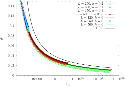
For a general system, the largest eigenvalue $\lambda_{\textrm{\tiny max}}$ can be obtained by taking the limit $n\to+\infty$ of the Rényi entropies, which gives $S_{A}^{(n)}\to-\log\lambda_{\textrm{\tiny max}}$ . In the rainbow CFT model and for an interval $A=(x_{0},L)$ adjacent to the boundary of the segment $(-L,L)$, we can take the limit $n\to+\infty$ of the result found in [13], which gives

$$-\log\lambda_{\textrm{\tiny max}}\,=\,\frac{1}{12}\,\log\tilde{\mathcal{L}}_{A}+\frac{Q_{\infty}}{2}\,,$$ (86)

where we have introduced the following effective length

$$\tilde{\mathcal{L}}_{A}\equiv\frac{8\tilde{L}}{\pi}\,e^{\sigma(x_{0})}\,\,\sin\bigg(\frac{\pi\tilde{\ell}}{2\tilde{L}}\bigg)\,=\,\frac{8}{\pi}\,e^{-h|x_{0}|}\;\frac{e^{hL}-1}{h}\;\cos\left(\frac{\pi}{2}\;\frac{e^{h|x_{0}|}-1}{e^{hL}-1}\right)\,\equiv\,L\,\tilde{L}_{A}\,,$$ (87)

being $\tilde{L}_{A}$ the function of $\lambda$ and $x_{0}/L$ given by

$$\tilde{L}_{A}\equiv\frac{8}{\pi}\,e^{-\lambda|x_{0}/L|}\;\frac{e^{\lambda}-1}{\lambda}\;\cos\left(\frac{\pi}{2}\;\frac{e^{\lambda|x_{0}/L|}-1}{e^{\lambda}-1}\right).$$ (88)

The numerical value of the constant $Q_{\infty}$ in (86) reads $Q_{\infty}=0.2797$, which has been obtained by taking the limit $n\rightarrow+\infty$ of the constants $Q_{n}$ introduced in [41] for the XX model (see also [42, 43]).

By using (86) and (87), it is straightforward to construct the following combination

$$-\log\lambda_{\textrm{\tiny max}}-\frac{1}{12}\log L\,=\,\frac{1}{12}\,\log\tilde{L}_{A}+\frac{Q_{\infty}}{2}\,.$$ (89)

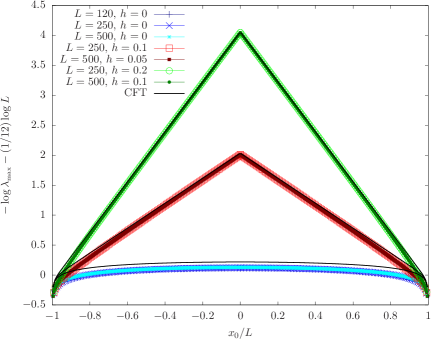
This analytic expression has been compared against the numerical values obtained from the lattice through (85) in the left panel of Fig. 7. The agreement is very good and it improves as $\lambda$ increases. In the homogenous case, i.e. for $\lambda=0$, a slight deviation is observed between the data points and the corresponding analytic curve. We expect that higher values of $L$ are needed in order to improve the matching with the CFT curve.

The subleading corrections to (86) can be analysed by considering

$$d_{0}\equiv-\log\lambda_{\textrm{\tiny max}}-\left(\frac{1}{12}\,\log\tilde{\mathcal{L}}_{A}+\frac{Q_{\infty}}{2}\right),$$ (90)

whose data point are shown in the right panel of Fig. 7. From the data corresponding to $\lambda=0$, it is evident that the agreement with the CFT curve improves as $L$ increases. Although the subleading corrections (90) strongly depend on the underlying model (see e.g. [42, 43] for homogenous cases), in the right panel of Fig. 7 we have compared the data point with the following analytic curve

$$d_{0}^{\textrm{\tiny CFT}}=-\,\frac{\pi^{2}}{12\,\log(\tilde{\mathcal{L}}_{A}/2)}\,,$$ (91)

which has been obtained from (60) with $c=1$ and (87). The qualitative behaviour of the lattice data in the right panel of Fig. 7 is nicely captured by (91), except for a vertical shift, which could be attributed to the fact that the $O(1)$ term in (60) is not universal.

7.2.2 First gap in the entanglement spectrum.

Interesting quantities which characterise the entanglement spectrum for a particular configuration are the gaps between the eigenvalues of the reduced density matrix. In the CFT analysis of §5 the gaps with respect to the largest eigenvalue are provided by (61) for the inhomogeneous models that we are considering.

Given the ordered sequence $E_{0}<E_{1}<E_{2}<\dots$ of the entanglement energies, in the following we focus on the first gap in the entanglement spectrum, namely

$${\cal E}_{1}\equiv E_{1}-E_{0}=2\varepsilon_{\frac{1}{2}}\,,$$ (92)

where in the last step the relation $\varepsilon_{-\frac{1}{2}}=-\varepsilon_{-\frac{1}{2}}$ has been used. The gap ${\cal E}_{1}$ gives also the slopes of the straight dashed-dotted lines in Fig. 6.

The linearity of the single body entanglement energies $\varepsilon_{i}$ implies that the other gaps ${\cal E}_{k}$ are multiples of ${\cal E}_{1}$.

Figure 8: Left: The inverse of the first gap in the entanglement spectrum $2\pi^{2}/{\cal E}_{1}$ in terms of the logarithm of the effective block size $\log\tilde{\mathcal{L}}_{A}$, defined in (87), for $L=250$. The straight dashed-dotted line has slope one, as predicted by the analytic formula (94). The inset shows a zoom in the region close to the origin, which highlights the numerical estimation of the intercept, which gives $\log\gamma\approx 1.9$. Right: The combination $2\pi^{2}/{\cal E}_{1}-\log L$ (see (94)) in terms of $x_{0}/L$ for rainbow chains having either $L=250$ or $L=500$, with values of $h$ properly chosen in order to emphasize the collapse of the numerical data having the same $\lambda=hL$. By employing the same value of $\gamma$ obtained numerically in the left panel, an excellent agreement is observed with the theoretical prediction (88).

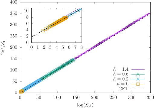
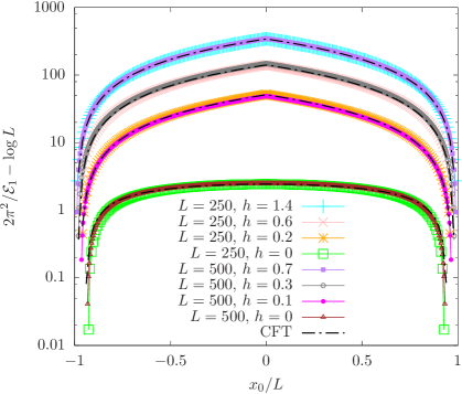
The CFT analysis in §5 predicts that ${\cal E}_{1}$ is given by (61) specified to our case, where $\Delta_{1}=1$ and the effective length (87) must be employed. The result reads

$${\cal E}_{1}=\frac{2\pi^{2}}{\log(\gamma\tilde{\mathcal{L}}_{A})}\,,$$ (93)

which tells us that ${\cal E}_{1}$ is inversely proportional to the logarithm of the effective length (87) and we have introduced a non universal constant $\gamma$ that can be estimated through the numerical analysis. We find it more convenient to write (93) as follows

$$\frac{2\pi^{2}}{{\cal E}_{1}}\,=\,\log\tilde{\mathcal{L}}_{A}+\log\gamma\,=\,\log L+\log\tilde{L}_{A}+\log\gamma\,.$$ (94)

In Fig. 8 we show the numerical data collected for various rainbow chains in order to check the validity of the analytic prediction (94), where $\tilde{L}_{A}$ is given by (88). The agreement with the data point is excellent. The constant $\gamma$ in (94) is non universal and it has been estimated through a global fit of the data shown in the left panel of Fig. 8, finding $\log\gamma\approx 1.9$ (see the inset). This numerical value agrees with the constant $-\,\psi(1/2)\simeq 1.963$, where $\psi(x)$ is the digamma function, obtained in [42] in the analysis of the subleading correction to the Rényi entropies of an interval in the infinite XX chain in the limit $n\to+\infty$ of the Rényi index. It would be interesting to provide a derivation of the constant $\gamma$ through analytical techniques.

In the right panel of Fig. 8 we have considered the combination $2\pi^{2}/{\cal E}_{1}-\log L$ in terms of $x/L$ for rainbow chains of two different lengths, showing that the data points collapse on the analytic expression given by $\log\tilde{L}_{A}+\log\gamma$, which corresponds to a family of curves parameterised by $\lambda=hL$, as one can observe from (88).

We find it worth discussing the expression (94) in some interesting special regimes.

In the homogenous case, i.e. for $h=0$, the following result of [24] is recovered

$$\frac{2\pi^{2}}{\mathcal{E}_{1}}\,=\,\log\left[L\,\sin\bigg(\frac{\pi(L-x_{0})}{2L}\bigg)\right]+\log(8\gamma/\pi)\,,$$ (95)

which corresponds to the $j=1$ case of (25) and tells us that the gap $\mathcal{E}_{1}$ is inversely proportional to the logarithm of the chord length of the block.

When $A$ is half of the entire segment, $x_{0}=0$ and the effective length (87) simplifies to $\tilde{\mathcal{L}}_{A}=8\tilde{L}/\pi$; therefore (94) becomes

$$\frac{2\pi^{2}}{\mathcal{E}_{1}}\,=\,\log L+\log\left(\frac{e^{\lambda}-1}{\lambda}\right)+\log(8\gamma/\pi)\,,$$ (96)

which agrees with the ansatz made in Eq. (21) of [10].

Finally, in the regime defined by $\lambda\gg 1$ with $|x_{0}|/L$ fixed, we have that (94) gives

$$\frac{2\pi^{2}}{\mathcal{E}_{1}}\,\simeq\,h\big(L-|x_{0}|\big)-\log h+\log(8\gamma/\pi)\,.$$ (97)

In particular, for $x_{0}=0$ the r.h.s. of this expression further simplifies to ${\cal E}_{1}\simeq 2\pi^{2}/(hL)$, which is the result found in [11] and employed to interpret the ground state of the rainbow chain as a thermofield double.

7.3 A contour for the entanglement entropies

Entanglement contours are natural concepts to study in the analysis of the bipartite entanglement. These quantities attempt to quantify the contribution of a single site (or of a point in the continuum) in the subsystem to the entanglement of the bipartition. The contours for the entanglement entropies in some free and homogeneous models on the lattice have been studied in [26, 27, 28, 29].

In the strong coupling limit of the rainbow chain, the question addressed by the contour for the entanglement entropy has a natural answer. Indeed, since the ground state in this regime is a valence bond state, the entanglement entropy can be evaluated by counting the bonds which are broken by the partition. In particular, each broken bond provides a contribution of $\log 2$ to the entanglement entropy, which is obtained by the summing of all these contributions [9, 10, 11]. Thus, for each site in the block, either it contributes with $\log 2$ to the entanglement or it does not.

In the following analysis we consider a contour for the entanglement entropies in the rainbow chain which can be employed in the entire range of the parameters and captures the expected feature of the strong coupling regime.

For a free fermion on the lattice, the Rényi entropies of a subsystem $A$ are computed from the the eigenvalues $\{\nu_{k}\}$ of the correlation matrix $C_{ij}=\langle c^{\dagger}_{i}c_{j}\rangle$ restricted to the subsystem $A$ (i.e. for $i,j\in A$) as follows [23]

$$S^{(n)}_{A}=\,\frac{1}{1-n}\,\sum_{k}\log(\nu_{k}^{n}+(1-\nu_{k})^{n})\,.$$ (98)

The entanglement entropy corresponds to the limit $n\to 1$ of this expression.

Denoting by $\{\psi_{k,i}\}$ the components of the normalised eigenvector associated to the eigenvalue $\nu_{k}$, it is natural to construct the contour function $s^{(n)}_{A}(i)$ as follows [27]

$$s^{(n)}_{A}(i)={1\over 1-n}\sum_{k}|\psi_{k,i}|^{2}\,\log(\nu_{k}^{n}+(1-\nu_{k})^{n})\,,\;\;\qquad\;\;i\,\in\,A\,.$$ (99)

Since $\sum_{i\in A}|\psi_{k,i}|^{2}=1$ for every $k$, it is straightforward to check that (99) satisfies the conditions $\sum_{i}s^{(n)}_{A}(i)=S^{(n)}_{A}$. Moreover, $s^{(n)}_{A}(i)\geqslant 0$ for every $i\in A$. These two conditions are minimal requirements for a contour function for the entanglement entropies. Other properties have been introduced in [27] to reduce the large arbitrariness of this construction, but a complete list characterising the contour for the entanglement entropies in a unique way is not known.

In our analysis we have adapted the construction of [27] to the rainbow chain.

For homogeneous critical systems in the continuum limit, the profiles of the contour function for the entanglement entropies have been proposed in [29] (by employing the CFT analysis of [24]) for a particular class of configurations which includes also the one we are considering, namely an interval adjacent to the boundary of a segment. As for the inhomogeneous critical systems discussed above, whose continuum limit is described by a CFT in a curved background, a contour function for the entanglement entropies of the configuration of our interest has been proposed §6: it is given by (66), where the function $\mathcal{S}_{A}(x)$ has been defined in (67).

By employing the inverse of (21) and (38), we can specify $\mathcal{S}_{A}(x)$ in (67) for the rainbow model, finding

$$\mathcal{S}_{A}(x)\;=\;\frac{\pi}{2L}\;\frac{\lambda}{e^{\lambda}-1}\;\,\frac{e^{\lambda|x/L|}\,\cos\big(\tfrac{\pi}{2}\,\tfrac{(e^{\lambda|x_{0}/L|}-1)\,\textrm{sign}(x_{0}/L)}{e^{\lambda}-1}\big)}{\sin\big(\tfrac{\pi}{2}\,\tfrac{(e^{\lambda|x/L|}-1)\,\textrm{sign}(x/L)}{e^{\lambda}-1}\big)-\sin\big(\tfrac{\pi}{2}\,\tfrac{(e^{\lambda|x_{0}/L|}-1)\,\textrm{sign}(x_{0}/L)}{e^{\lambda}-1}\big)}\,,$$ (100)

which is the inverse of (75), as also stated by (69). From (100) it is straightforward to observe that $L\,s_{A}^{(n)}(x)$ is a function of $x/L$ parameterised by $\lambda$ and $x_{0}/L$.

The function (100) diverges linearly close to the entangling point, i.e. for $x\to x_{0}^{+}$, as already remarked through the more general expansion (68), and it gets a finite value at the other endpoint, which coincides with the endpoint of the segment.

Figure 9: Left: Contour function for the entanglement entropy $s_{A}(x)$ of half rainbow chains with $L=100$ and different values of $h$. The continuous solid lines represent the CFT prediction given by (66), with $n=1$ and $C_{1}=0$, and (102). A plateau occurs for intermediate values of $x$ and finite $h$, whose height is $h/6$. Close to the entangling point the linear divergence (68) with $x_{0}=0$ is observed, while near the other endpoint (which is also the endpoint of the segment) non universal parity oscillations become relevant. Right: $L\,s_{A}(x)$ as a function of $x/L$ for different values of $L$ and $h$ suitably chosen in order to deal with the fixed values of $\lambda=hL$ reported near the corresponding curves.

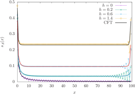
We find it worth considering first the contour function for the entanglement entropies given by (66) and (100) in some special regimes. We have set $C_{n}=0$ throughout our numerical analysis.

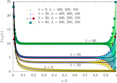
In the homogenous case ($h=0$), we have that $\tilde{x}=x$; therefore $\tilde{L}=L$ and $\tilde{x}_{0}=x_{0}$. In this regime the function (100) simplifies to the expression found in [24], namely

$$\mathcal{S}_{A}(x)=\frac{\pi}{2L}\;\frac{\cos(\pi x_{0}/(2L))}{\sin(\pi x/(2L))-\sin(\pi x_{0}/(2L))}\,.$$ (101)

The contour function for the entanglement entropies of this configuration has been also studied in [29] in the homogeneous harmonic chain with Dirichlet boundary conditions imposed at the endpoints of the segment. For this harmonic chain the CFT prediction (101) (which does not depend on the specific boundary conditions imposed at the endpoints of the segment) does not capture the lattice data for the entire interval. In particular, a good agreement with the data points is observed near the entangling point (i.e. for $x\simeq x_{0}^{+}$) but a large deviation from (101) occurs as $x$ approaches the boundary, i.e. where the data points are sensible to the boundary condition imposed at the endpoint of the segment.

Another interesting special case corresponds to a block $A$ given by half of the entire segment. In this case $x_{0}=0$ and (100) becomes

$$\mathcal{S}_{A}(x)=\frac{\pi h\,e^{hx}}{2(e^{hL}-1)}\;\bigg[\sin\left(\frac{\pi}{2}\frac{e^{hx}-1}{e^{hL}-1}\right)\bigg]^{-1},$$ (102)

where $x\in(0,L)$. In the regime of $hL\gg 1$ with $x/L$ kept constant, the argument of the sine function becomes $\tfrac{\pi}{2}\,e^{-h(L-x)}$, therefore the expression in (102) simplifies to $\mathcal{S}_{A}(x)\simeq h$. In the homogenous case, i.e. for $h=0$, the function (102) simplifies further to

$$\mathcal{S}_{A}(x)=\frac{\pi}{2L\,\sin(\pi x/(2L))}\,,$$ (103)

which can be obtained also by setting $x_{0}$ into (101).

The results of our numerical analysis for the contour of the entanglement entropy when $x_{0}=0$ have been reported in Fig. 9, where the left panel shows the contour function $s_{A}(x)$ for $L=100$ and different values of $h$. The solid lines correspond to the CFT prediction given by (66) for $n=1$ and (102) with $C_{1}=0$. The agreement between the numerical data and the analytic expression in the continuum is remarkably good already at this value of $L$. In the right panel of Fig. 9 we consider rainbow chains of different lengths and various values of $h$. As the CFT prediction (102) suggests, it is convenient to plot $L\,s_{A}(x)$ in terms of $x/L$ because the resulting curve is parameterised only by $\lambda$. This prediction is confirmed by the numerical data shown in the right panel of Fig. 9.

Figure 10: Left: Contour functions for the entanglement entropy $s_{A}(x)$ and $s_{B}(x)$ of two complementary blocks $A=(x_{0},L)$ and $B=(-L,x_{0})$ separated by one entangling point at $x_{0}<0$. The rainbow chains have $L=100$, $x_{0}=-50$ and different values of $h$. The blue and red solid lines correspond to the CFT prediction for $A$ and $B$ respectively, given by (66), with $n=1$ and $C_{1}=0$, and (100). The linear divergence (68) is observed in the neighbourhood of the entangling point, while finite parity oscillations occur close to the boundaries of the segment. The dashed horizontal lines correspond to $h/6$, which is the height of the plateau predicted by the analytic formula. In the regime $\lambda\gg 1$ the contour function vanishes exponentially in the inactive region $(x_{0},-x_{0})$, as found analytically in (105), confirming the expectation that this region does not contribute to the entanglement between $A$ and $B$ because the corresponding bonds do not cross the entangling boundary. Parity oscillations occur also for low non vanishing values of $h$ near the physical boundaries. Right: $L\,s_{A}(x)$ and $L\,s_{B}(x)$ in terms of $x/L$ for two different values of $L$, with $h$ suitably chosen in order to deal with fixed values of $\lambda=hL$.

The linear divergence (68) close to the entangling point, which is the universal prediction of the CFT analysis, is clearly observed from the numerical data. As for the behaviour of the contour function for the entanglement entropy close to the other endpoint of the interval $A$, which coincides with the endpoint of the segment, the finite value of $s_{A}(x)$ is captured by the data points within some range established by non universal parity oscillations. From the right panel of Fig. 9 we observe that these oscillations provide a definite profile under scaling. It would be interesting to have some analytical comprehension of these oscillations.

Figure 11: Left: Contour function for the entanglement entropies $s_{A}^{(n)}(x)$ of an interval $A=(x_{0},L)$ adjacent to the boundary, with $x_{0}=-50$ and $L=125$. The solid lines represent the CFT prediction given by (66), with $C_{n}=0$, and (100). The horizontal dashed lines correspond to $(1+\tfrac{1}{n})\,h/12$, which are the heights of the plateaux obtained from the analytic formula. The amplitude of the parity oscillations increases as the Rényi index $n$ increases. Right: $L\,s^{(n)}_{A}(x)/(1+\tfrac{1}{n})$ as a function of $x/L$ for two different system sizes and $x_{0}/L=-0.4$, with $h$ properly chosen in order to emphasize the collapse of the numerical data having the same $\lambda=hL$.

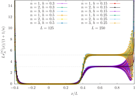
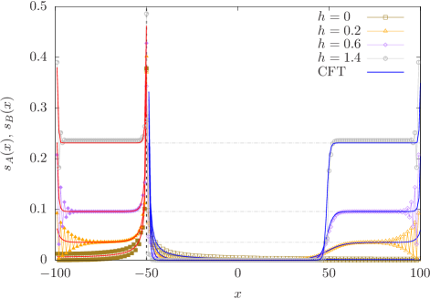
The most interesting behaviour for the contour function of the entanglement entropies is observed when $x_{0}\neq 0$. In this case the CFT analytic formula is given by (66) with $C_{n}=0$ and (100). The essential feature is captured in the regime of $\lambda\gg 1$ with $x/L$ constant and $x\neq x_{0}$, where (100) becomes

$$\mathcal{S}_{A}(x)\,\simeq\,\frac{h}{\textrm{sign}(x)-\textrm{sign}(x_{0})\,e^{-h(|x|-|x_{0}|)}}\,.$$ (104)

When $x_{0}>0$, this expression further simplifies to $\mathcal{S}_{A}(x)\simeq h$, which is the same plateau already found for $x_{0}=0$.

The intriguing behaviour is observed for $x_{0}<0$, where (104) gives

$$\mathcal{S}_{A}(x)\,\simeq\,\left\{\begin{array}[]{ll}h\,e^{-h(|x_{0}|-|x|)}&-|x_{0}|<|x|<|x_{0}|\,,\\ \rule{0.0pt}{17.07182pt}h&|x_{0}|<x<L\,,\end{array}\right.$$ (105)

which is the inverse of (82), as expected from (69). We remark that (105) quantifies the expected feature of the contour function for the entanglement entropies in the strong coupling regime mentioned in the beginning of this section (see also the discussion below (82)). Indeed, since the inactive zone $(-|x_{0}|,+|x_{0}|)$ contains bonds which stay inside the block $A$, it does not contribute to the bipartite entanglement between $A$ and $B$. Instead, the active zone $(|x_{0}|,L)$, which contains bonds connecting $A$ to its complement $B$, is entirely responsible for the entanglement between $A$ and $B$. Moreover, notice that the plateau profile of the contour function in the active zone $(|x_{0}|,L)$ of $A$ is the same profile observed for the contour function in $B$ in the intermediate region.

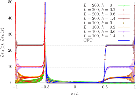
In Fig. 10 we have collected the data for the contour function of the entanglement entropy in various rainbow chains when $x_{0}<0$. In order to highlight the role of the active zone mentioned above, we have shown the contour function for both $A=(x_{0},L)$ and its complement $B=(-L,x_{0})$. Notice that, because of the symmetry with respect to the origin, the contour function for $B=(-L,x_{0})$ when $x_{0}<0$ can be obtained by reflecting the contour function of the block $(-x_{0},L)$. In the left panel of Fig. 10, the contour functions $s_{A}(x)$ and $s_{B}(x)$ are shown for a fixed configuration given by $L=100$ and $x_{0}=-50$, while in the right panel various configurations have been considered in order to highlight the fact that $L\,s_{A}(x)$ and $L\,s_{B}(x)$ are functions of $x/L$ parameterised by $\lambda$. In the neighbourhood of the endpoints of the intervals $A$ and $B$, the behaviour is qualitatively like the one discussed for $x_{0}$ (see Fig. 9): the linear divergence (68) near the entangling point $x_{0}$ and finite parity oscillations whose amplitudes increase as $x$ approaches the boundaries of the segment. The new feature of Fig. 10 is the behaviour of the contour function in the neighbourhood of the point $-x_{0}$ in $A$, which separates the active zone from the inactive zone. A remarkable agreement is observed with the CFT analytic formula given by (66) with $C_{n}=0$ and (100) for both the contour functions $s_{A}(x)$ and $s_{B}(x)$. Notice that, close to the boundaries of the segment, the CFT curve is in the middle of the oscillations. We find vey remarkable that the CFT expression for the contour function is able to capture the behaviour of the numerical data for these free fermionic chains along all the entire block. This does not happen for the harmonic chains [29].

Figure 12: Entanglement entropy $S_{A}$ (increasing bluish points) and first gap in entanglement spectrum ${\cal E}_{1}/\tfrac{\pi^{2}}{3}$ (decreasing greenish points), along with their product (black points). The data points confirm the validity of (106) with $n=1$. Rainbow chains with either $L=50$ or $L=250$ have been employed, being $A=(x_{0},L)$ of size $\ell$. Notice the symmetry between $S_{A}$ and ${\cal E}_{1}/\tfrac{\pi^{2}}{3}$ (in logarithmic scale) for the same chain.

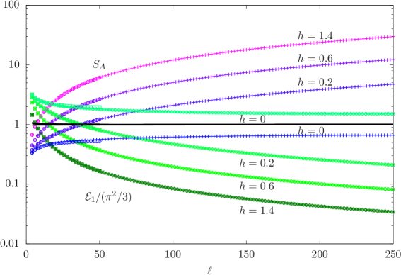
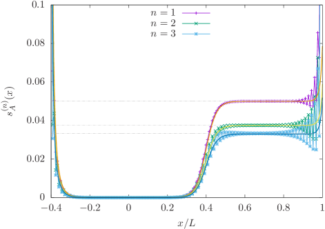
Considering again an interval $A=(x_{0},L)$ with $x_{0}<0$, in Fig. 11 we have reported the contour function $s_{A}^{(n)}(x)$ for the Rényi entropies $S_{A}^{(n)}$, in order to study the role of the Rényi index $n$. The essential features discussed for the contour function $s_{A}(x)$ in Fig. 10 are observed also for $s_{A}^{(n)}(x)$ with $n\geqslant 2$. We find it worth remarking that, from the data points we can clearly observe that the amplitude of the parity oscillations increases as the Rényi index $n$ increases. Moreover, in the right panel of Fig. 11 we show that, by considering $L\,s_{A}^{(n)}(x)/(1+\tfrac{1}{n})$, the data points for different rainbow chains collapse on a function of $x/L$ parameterised by $\lambda$ and $x_{0}/L$. The CFT prediction for this function can be read from (100) and it nicely agrees with the lattice data.

Figure 13: Couplings $\beta_{i}$ of the entanglement hamiltonian (71) and contour function for the entanglement entropy $s_{A}(x)$ in terms of the position inside the subsystem ($i=x$), for blocks $A=(x_{0},L)$ with $L=40$, along with their product. The logarithmic scale highlights the validity of the relation $\beta_{i}\,s_{A}(x)=\pi/3$ (see (107) with $n=1$). The parity oscillations in the contour have been removed by applying a local smoothing convolution. Left: Configurations with $x_{0}=0$. Right: Configurations with $x_{0}/L=-0.5$.

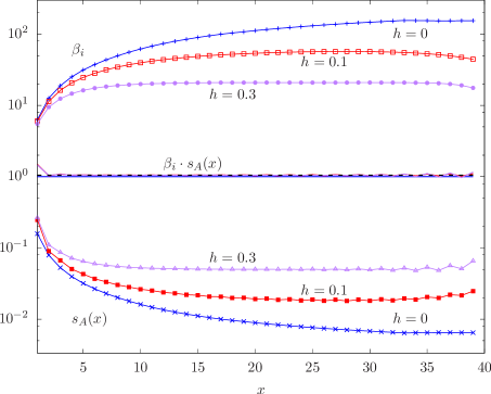
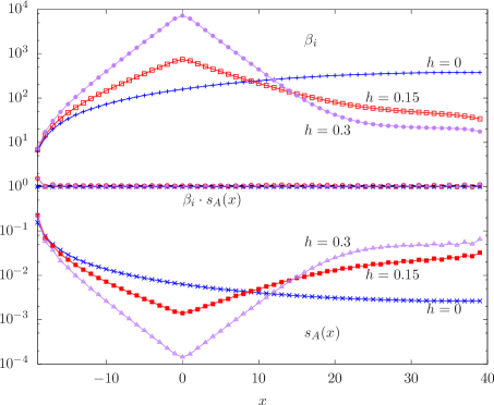
In the final part of our numerical analysis of the rainbow chain, we find it worth considering the CFT relation (62) involving the Rényi entropies $S_{A}^{(n)}$ and the gaps $\mathcal{E}_{k}$ in the entanglement spectrum, In particular, focussing on the first gap $\mathcal{E}_{1}$, which has been studied numerically in §7.2.2 for the rainbow chain, from (62) we have

$$\mathcal{E}_{1}\,S^{(n)}_{A}\,\simeq\,\frac{\pi^{2}}{6}\left(1+\frac{1}{n}\right),$$ (106)

where the subleading corrections have been neglected. In Fig. 12 we show numerical data to check (106) for $n=1$ in various rainbow chains (see also Fig. 8 of [10]).

Another interesting CFT relation that we find worth checking numerically is (70). For rainbow chains $c=1$; therefore (70) becomes

$$\big[2\pi\beta_{A}(x)\big]\,s^{(n)}_{A}(x)\,\simeq\,\frac{\pi}{6}\left(1+\frac{1}{n}\right),$$ (107)

up to subleading corrections. In Fig. 13 different rainbow chains have been considered to check the relation (107) numerically and a good agreement is observed.

8 Conclusions

The analysis of operators and other related quantities underlying the measures of the bipartite entanglement is an important task in order to improve our comprehension of entanglement in many body quantum systems and quantum field theory.

In this manuscript we have considered some inhomogeneous static critical systems in one spatial dimension whose continuum limit is described by a CFT in a static curved background characterised by a metric which is a Weyl rescaling of the flat metric that only depends on the space variable. In these models, we have considered a subsystem given by an interval adjacent to the boundary of a segment with finite length. The same boundary condition is imposed at the endpoints of the segment. For this configuration we have studied the entanglement hamiltonian, the entanglement spectrum and an entanglement contour for the entanglement entropies. Our CFT analysis extends some results obtained in [24, 29] in flat spacetime and it reproduces the entanglement entropies for this configuration obtained through the twist fields method in [6, 13].

In order to check numerically our CFT predictions through lattice computations, we have considered the rainbow chain, which is a free fermion model in a segment where the hopping amplitudes decay exponentially going from the center of the chain towards the boundaries in a symmetric way [9, 10, 11, 13]. Specialising our CFT formulas to the rainbow model, we have obtained an excellent agreement with the lattice data for all the quantities that we have considered: the couplings in the ansatz (71) for the entanglement hamiltonian (Figs. 3 and 5), the largest eigenvalue of the reduced density matrix (Fig. 7), the first gap in the entanglement spectrum (Fig. 8) and the contour function for the entanglement entropies (Figs. 9, 10 and 11).

Our numerical analysis of the entanglement hamiltonian is based on the ansatz (71), which includes only the coupling between nearest neighbours sites in the subsystem. It would be interesting to consider also couplings between sites at generic distance and, given the results of [23, 25] for homogeneous free fermions, we expect that their amplitudes are much smaller than the ones between nearest neighbours.

As for the contour for the entanglement entropies, we find it remarkable that our analytic formulas predict the correct behaviour for the entire interval, although they do not depend on the boundary condition imposed at the endpoints of the segment. This is not case for the harmonic chain [29]. It would be interesting to understand better the role of the boundary conditions in the contour function for the entanglement entropies. Another interesting feature observed in our numerical analysis of the contour for the entanglement entropies is given by the parity oscillations, whose amplitude, which depends both on the position and on the inhomogeneity parameter, increases near the boundary of the segment. Providing an analytic treatment of these parity oscillations could be an interesting question for future studies. Besides the issues related to the specific models, let us remind that a complete list of properties which defines the contour for the entanglement entropies in unique way is not available [27, 29].

Our analysis can be extended in various directions. For instance, more complicated configurations or curved backgrounds corresponding to other inhomogeneous critical systems can be considered [44]. Moreover, since our analytic formulas can be applied also for inhomogeneous models with arbitrary central charge, it would be interesting to check numerically their validity for some models having $c\neq 1$.

Another important direction for future studies consists in extending the analysis described in this manuscript to inhomogeneous systems defined in two or three spatial dimensions.

Appendices

Appendix A Rényi entropies and Liouville action

In this appendix we describe an argument employed in the discussion reported in the beginning of §5 to obtain (50).

Given a two dimensional manifold $\mathcal{M}$ whose boundary $\partial\mathcal{M}$ can be made of an arbitrary number of disjoint components, let us denote by $(\mathcal{M},g)$ the spacetime defined by introducing a two dimensional euclidean metric $g_{\mu\nu}$ on $\mathcal{M}$. In the following we consider two spacetimes $(\mathcal{M},g)$ and $(\mathcal{M},\hat{g})$ whose metrics are related through a Weyl factor, namely $g_{\mu\nu}=e^{2\sigma}\hat{g}_{\mu\nu}$. The partition functions $\mathcal{Z}[\mathcal{M},g]$ and $\mathcal{Z}[\mathcal{M},\hat{g}]$ of a 2D CFT with central charge $c$ defined respectively on $(\mathcal{M},g)$ and on $(\mathcal{M},\hat{g})$ are related as follows [37, 38]

$$\mathcal{Z}[\mathcal{M},g_{\mu\nu}]\,=\,e^{\frac{c}{6}\,S_{L}[\,\sigma\,;\,\mathcal{M},\,\hat{g}_{\mu\nu}\,]}\,\mathcal{Z}[\mathcal{M},\hat{g}_{\mu\nu}]\,,$$ (108)

where $S_{L}[\,\sigma\,;\,\mathcal{M},\,\hat{g}_{\mu\nu}\,]$ is the Liouville action on $(\mathcal{M},\hat{g})$, which is given by

$$S_{L}[\,\sigma\,;\,\mathcal{M},\,\hat{g}_{\mu\nu}\,] \,\equiv\, \frac{1}{4\pi}\int_{\mathcal{M}}\Big(\,\hat{g}^{\mu\nu}\partial_{\mu}\sigma\,\partial_{\nu}\sigma+\widehat{R}\,\sigma+\mu\,e^{2\sigma}\Big)\sqrt{\hat{g}}\,d^{2}x$$ (109)

$$+\frac{1}{2\pi}\int_{\partial\mathcal{M}}\Big(\widehat{K}\,\sigma+\tilde{\mu}\,e^{\sigma}\Big)\sqrt{\hat{h}}\,d\lambda\,,$$

being $\widehat{R}$ the scalar curvature of the metric $\hat{g}_{\mu\nu}$. The metric on $\partial\mathcal{M}$ is the metric induced from the embedding. The element of arc length on $\partial\mathcal{M}$ is $\sqrt{\hat{h}}\,d\lambda$ and $\widehat{K}$ is the extrinsic curvature of $\partial\mathcal{M}$. The constants $\mu$ and $\tilde{\mu}$ are respectively the bulk cosmological constant and boundary cosmological constant.

The Liouville theory is a paradigmatic model of irrational CFT whose analysis led to important advances in the comprehension of two dimensional CFTs [45, 46, 47]. It is worth mentioning that the regularization procedure discussed in §2 and §5 following [17, 24], which is based on the removal of infinitesimal disks centered in the positions of the local operators, has been also employed in the path integral approach to the correlation functions in Liouville theory [45, 48].

We are interested in the case of $\mathcal{M}=\mathbb{S}\setminus\cup_{j}\mathbb{D}_{\epsilon}(x_{j})$ is a vertical strip $\mathbb{S}$ from which small disks $\mathbb{D}_{\epsilon}(x_{j})$ of radius $\epsilon$ centered at the entangling points (which can be made by several disjoint intervals in the segment $(-L,L)$) have been removed. We remark that, since $x_{j}$ correspond to the entangling points, we have that $x_{j}\neq-L$ and $x_{j}\neq L$. Thus, the boundary $\partial\mathcal{M}$ is the union of the vertical lines given by $x=-L$ and $x=L$, and of all the circumferences $\partial\mathbb{D}_{\epsilon}(x_{j})$ around the entangling points $x_{j}$.

When $\hat{g}_{\mu\nu}=\delta_{\mu\nu}$ is the flat metric, we have $\widehat{R}=0$ in (109). As for the extrinsic curvature of $\partial\mathcal{M}$ in the flat background, $\widehat{K}=0$ along the vertical straight lines at $x=-L$ and $x=L$, while $\widehat{K}=-1/\epsilon$ along $\partial\mathbb{D}_{\epsilon}(x_{j})$. Thus, the boundary term containing the extrinsic curvature in (109) provides non vanishing contributions only along the infinitesimal circumferences $\partial\mathbb{D}_{\epsilon}(x_{j})$. For each of them we have

$$\lim_{\epsilon\,\to\,0}\,\frac{1}{2\pi}\oint_{\partial\mathbb{D}_{\epsilon}(x_{j})}\widehat{K}\,\sigma\,d\lambda\,=\,-\,\sigma(x_{j})\,,$$ (110)

which can be found by assuming that $\sigma$ is smooth in a neighbourhood of the entangling point and using that $d\lambda=\epsilon\,d\theta$, being $\theta\in[0,2\pi)$ the angular coordinate along $\partial\mathbb{D}_{\epsilon}(x_{j})$.

In this manuscript we focus on the simplest configuration where $A=(x_{0},L)$ is a single interval adjacent to the boundary of the strip and $\hat{g}_{\mu\nu}=\delta_{\mu\nu}$ is the flat metric. In this case $\mathcal{M}=\mathbb{S}\setminus\mathbb{D}_{\epsilon}(x_{0})$, as discussed in §2. The spacetime $(\mathcal{M},\delta)$, which corresponds to both $A=(x_{0},L)$ and its complement $B=(-L,x_{0})$, is shown in the left panel of Fig. 1.

In order to find the Rényi entropies, we need to consider the following ratio

$${\rm Tr}\rho_{A}^{n}\,=\,\frac{\mathcal{Z}[\mathcal{M}_{n},g_{\mu\nu}]}{\big(\mathcal{Z}[\mathcal{M},g_{\mu\nu}]\big)^{n}}\,=\,e^{\frac{c}{6}(S_{L}[\,\sigma\,;\,\mathcal{M}_{n},\,\delta_{\mu\nu}\,]-\,n\,S_{L}[\,\sigma\,;\,\mathcal{M},\,\delta_{\mu\nu}\,])}\ \frac{\mathcal{Z}[\mathcal{M}_{n},\delta_{\mu\nu}]}{\big(\mathcal{Z}[\mathcal{M},\delta_{\mu\nu}]\big)^{n}}\,,$$ (111)

where $\mathcal{Z}[\mathcal{M}_{n},g_{\mu\nu}]$ is the partition function of the 2D CFT on the $n$-sheeted Riemann surface obtained by gluing $n$ copies of $\mathcal{M}$ cyclically along the upper and the lower edges of $A$ [17, 24]. The final expression in (111) has been obtained by using (108). In the case we are considering, $\partial\mathcal{M}_{n}$ includes $n$ vertical straight lines corresponding to $x=-L$ and $n$ vertical straight lines corresponding to $x=L$ coming from the different copies of $\mathcal{M}$. Because of the gluing procedure, $\partial\mathcal{M}_{n}$ also includes a closed $n$-covering $\partial\mathbb{D}^{n}_{\epsilon}(x_{0})$ of the circumference $\partial\mathbb{D}_{\epsilon}(x_{0})$. In particular, $\partial\mathbb{D}^{n}_{\epsilon}(x_{0})$ has radius $\epsilon$ and its length is $2\pi n\epsilon$. Thus, since $\widehat{K}=-1/\epsilon$ along $\partial\mathbb{D}^{n}_{\epsilon}(x_{0})$, we have

$$\lim_{\epsilon\,\to\,0}\,\frac{1}{2\pi}\oint_{\partial\mathbb{D}^{n}_{\epsilon}(x_{0})}\widehat{K}\,\sigma\,d\lambda\,=\,-\,n\,\sigma(x_{0})\,.$$ (112)

Since in the manuscript we have considered $\sigma=\sigma(x)$ (see (33)), in the Liouville action (109) the kinetic term, the bulk cosmological term and the boundary cosmological term along the straight lines at $x=-L$ and $x=+L$ provide diverging contributions because of the integration in the $y$ direction. Nonetheless, in (111) these divergencies in $S_{L}[\,\sigma\,;\,\mathcal{M}_{n},\,\delta_{\mu\nu}\,]$ cancel with the corresponding divergencies coming from the same kind of terms in $S_{L}[\,\sigma\,;\,\mathcal{M},\,\delta_{\mu\nu}\,]$. Instead, the boundary term in the Liouville action (109) containing the extrinsic curvature gives a finite contribution both in $S_{L}[\,\sigma\,;\,\mathcal{M}_{n},\,\delta_{\mu\nu}\,]$ and $S_{L}[\,\sigma\,;\,\mathcal{M},\,\delta_{\mu\nu}\,]$. By employing (110) and (112) notice that they also simplify in (111).

The above observations lead to the argument employed in the text below (49).

References

-
[1]
L. Amico, R. Fazio, A. Osterloh and V. Vedral, Rev. Mod. Phys. 80, 517 (2008);
J. Eisert, M. Cramer and M. Plenio, Rev. Mod. Phys. 82, 277 (2010);
P. Calabrese, J. Cardy and B. Doyon (Eds), J. Phys. A 42, 500301 (2009);
N. Laflorencie, Phys. Rep. 643, 1 (2016);
M. Rangamani and T. Takayanagi, Lect. Notes Phys. 931 (2017). -
[2]
R. Islam, R. Ma, P. Preiss, M. Tai, A. Lukin, M. Rispoli and M. Greiner, Nature 528, 77 (2015);
A. Kaufman, M. Tai, A. Lukin, M. Rispoli, R. Schittko, P. Preiss and M. Greiner, Science 353, 794 (2016);
J. Unmuth-Yockey, J. Zhang, P. Preiss, L.-P. Yang, S.-W. Tsai and Y. Meurice, Phys. Rev. A 96, 023603 (2017). - [3] G. Refael and J. Moore, Phys. Rev. Lett. 93, 260602 (2004).
[4]
G. Refael and J. Moore, J. Phys. A 42, 504010 (2009);
N. Laflorencie, Phys. Rev. B 72, 140408 (2005);
M. Fagotti, P. Calabrese and J. E. Moore, Phys. Rev. B 83, 045110 (2011);
G. Ramírez, J. Rodríguez-Laguna and G. Sierra, J. Stat. Mech. P07003 (2014);
P. Ruggiero, V. Alba and P. Calabrese, Phys. Rev. B 94, 035152 (2016). -
[5]
M. Campostrini and E. Vicari,
Phys. Rev. Lett. 102, 240601 (2009);
M. Campostrini and E. Vicari, Phys. Rev. A 82, 063636 (2010);
M. Campostrini and E. Vicari, Phys. Rev. A 81, 063614 (2010);
M. Campostrini and E. Vicari, J. Stat. Mech. 08020 (2010). - [6] J. Dubail, J.-M. Stéphan, J. Viti and P. Calabrese, SciPost Phys. 2, 002 (2017).
- [7] V. Eisler and D. Bauernfeind, Phys. Rev. B 96, 174301 (2017).
[8]
H. Ueda and T. Nishino, J. Phys. Soc. Japan 78, 014001 (2009);
H. Ueda, H. Nakano, K. Kusakabe and T. Nishino, Prog. Theor. Phys. 124, 389 (2010). - [9] G. Vitagliano, A. Riera and J. I. Latorre, New J. Phys. 12, 113049 (2010).
- [10] G. Ramírez, J. Rodríguez-Laguna and G. Sierra, J. Stat. Mech. P10004 (2014).
- [11] G. Ramírez, J. Rodríguez-Laguna and G. Sierra, J. Stat. Mech. P06002 (2015).
- [12] J. Rodríguez-Laguna, S.N. Santalla, G. Ramírez and G. Sierra, New J. Phys. 18, 073025 (2016).
- [13] J. Rodríguez-Laguna, J. Dubail, G. Ramírez, P. Calabrese and G. Sierra, J. Phys. A.: Math. Theor. 50, 164001 (2017).
- [14] X. Wen, S. Ryu and A. Ludwig, Phys. Rev. B 93, 235119 (2016).
[15]
O. Boada, A. Celi, J. I. Latorre, and M. Lewenstein, New J. Phys. 13, 035002 (2011);
J. Rodriguez-Laguna, L. Tarruell, M. Lewenstein, and A. Celi, Phys. Rev. A 95, 013627 (2017). - [16] C. Callan and F. Wilczek, Phys. Lett. B 333, 55 (1994).
- [17] C. Holzhey, F. Larsen and F. Wilczek, Nucl. Phys. B 424 (1994) 443.
- [18] G. Vidal, J. I. Latorre, E. Rico, and A. Kitaev, Phys. Rev. Lett. 90, 227902 (2003).
- [19] P. Calabrese and J. Cardy, J. Stat. Mech. P06002 (2004).
- [20] J. Cardy, O. Castro-Alvaredo and B. Doyon, J. Stat. Phys. 130: 129 (2008).
[21]
J. Bisognano and E. Wichmann, J. Math. Phys. 16, 985 (1975);
J. Bisognano and E. Wichmann, J. Math. Phys. 17, 303 (1976). -
[22]
P. Hislop and R. Longo,
Comm. Math. Phys. 84, 71 (1982);
H. Casini, M. Huerta and R. Myers, JHEP 1105 (2011) 036;
G. Wong, I. Klich, L. Pando Zayas and D. Vaman, JHEP 1312 (2013) 020;
H. Casini and M. Huerta, Class. Quant. Grav. 26 (2009) 185005. -
[23]
I. Peschel and M.-C. Chung,
J. Phys. A 32 (1999) 8419;
M.-C. Chung and I. Peschel, Phys. Rev. B 62, 4191 (2000);
M.-C. Chung and I. Peschel, Phys. Rev. B 64, 064412 (2001).
I. Peschel, J. Phys. A 36, L205 (2003);
I. Peschel, J. Stat. Mech. (2004) P06004;
I. Peschel and V. Eisler, J. Phys. A 42, 504003 (2009). - [24] J. Cardy and E. Tonni, J. Stat. Mech. (2016) 123103.
- [25] V. Eisler and I. Peschel, J. Phys. A: Math. Theor. 50, 284003 (2017).
- [26] A. Botero and B. Reznik, Phys. Rev. A 70, 052329 (2004).
- [27] Y. Chen and G. Vidal, J. Stat. Mech. P10011 (2014).
- [28] I. Frérot and T. Roscilde, Phys. Rev. B 92, 115129 (2015).
- [29] A. Coser, C. De Nobili and E. Tonni, J. Phys. A: Math. Theor. 50, 314001 (2017).
[30]
J. Eisert and M. Cramer,
Phys. Rev. A 72, 042112 (2005);
I. Peschel and Jize Zhao, J. Stat. Mech. (2005) P11002;
R. Orus, J. Latorre, J. Eisert and M. Cramer, Phys. Rev. A 73, 060303(R) (2006). -
[31]
H. Li and F. D. M. Haldane,
Phys. Rev. Lett. 101, 010504 (2008);
P. Calabrese and A. Lefevre, Phys. Rev A 78, 032329 (2008);
A. Läuchli, arXiv:1303.0741;
V. Alba, P. Calabrese and E. Tonni, arXiv:1707.07532. -
[32]
S. Furukawa, V. Pasquier and J. Shiraishi,
Phys. Rev. Lett. 102, 170602 (2009);
P. Calabrese, J. Cardy and E. Tonni, J. Stat. Mech. P11001 (2009);
P. Calabrese, J. Cardy and E. Tonni, J. Stat. Mech. P01021 (2011);
A. Coser, L. Tagliacozzo and E. Tonni, J. Stat. Mech. P01008 (2014);
C. De Nobili, A. Coser and E. Tonni J. Stat. Mech. P06021 (2015). - [33] H. Fujita, Y. Nakagawa, S. Sugiura and M. Oshikawa, arXiv:1705.05372.
- [34] L. Taddia, J. C. Xavier, F. C. Alcaraz and G. Sierra, Phys. Rev. B 88, 075112 (2013).
[35]
T. Truong and I. Peschel,
J. Phys. A: Math. Gen. 21, L1029 (1988);
B. Davies and P. Pearce, J. Phys. A: Math Gen. 23, 1295 (1990). - [36] C. Dasgupta and S.-K. Ma, Phys. Rev. B 22 1305 (1980).
- [37] A. Polyakov, Phys. Lett. B 103 (1981) 207.
- [38] O. Alvarez, Nucl. Phys. B 216 (1983) 125.
- [39] I. Cirac, D. Poilblanc, N. Schuch and F. Verstraete, Phys. Rev. B 83, 245134 (2011).
- [40] W. Press, S. Teukolsky, W. Vetterling and B. Flannery, Numerical Recipes in C. Cambridge University Press (1997). See also http://www.nr.com.
- [41] B.-Q. Jin and V. Korepin, J. Stat. Phys. 116, 79 (2004).
- [42] P. Calabrese and F. Essler, J. Stat. Mech. (2010) P08029.
- [43] M. Fagotti and P. Calabrese, J. Stat. Mech. (2011) P01017.
- [44] J. Rodríguez-Laguna, G. Sierra and E. Tonni, in progress.
- [45] A. Zamolodchikov and A. Zamolodchikov, Nucl. Phys. B 477 (1996) 577.
[46]
V. Fateev, A. Zamolodchikov and A. Zamolodchikov,
hep-th/0001012.
J. Teschner, arXiv:hep-th/0009138. - [47] A. Zamolodchikov and A. Zamolodchikov, arXiv:hep-th/0101152.
[48]
L. Takhtajan,
arXiv:hep-th/9409088;
P. Menotti and E. Tonni, Nucl. Phys. B 707 (2005) 321;
P. Menotti and G. Vajente, Nucl. Phys. B 709 (2005) 465;
P. Menotti and E. Tonni, Phys. Lett. B 633 (2006) 404;
P. Menotti and E. Tonni, JHEP 0606 (2006) 020;
P. Menotti and E. Tonni, JHEP 0606 (2006) 022.