Reduction Theorems for Hybrid Dynamical Systems

Abstract

This paper presents reduction theorems for stability, attractivity, and asymptotic stability of compact subsets of the state space of a hybrid dynamical system. Given two closed sets $\Gamma_{1}\subset\Gamma_{2}\subset\mathbb{R}^{n}$, with $\Gamma_{1}$ compact, the theorems presented in this paper give conditions under which a qualitative property of $\Gamma_{1}$ that holds relative to $\Gamma_{2}$ (stability, attractivity, or asymptotic stability) can be guaranteed to also hold relative to the state space of the hybrid system. As a consequence of these results, sufficient conditions are presented for the stability of compact sets in cascade-connected hybrid systems. We also present a result for hybrid systems with outputs that converge to zero along solutions. If such a system enjoys a detectability property with respect to a set $\Gamma_{1}$, then $\Gamma_{1}$ is globally attractive. The theory of this paper is used to develop a hybrid estimator for the period of oscillation of a sinusoidal signal.

I Introduction

Over the past ten to fifteen years, research in hybrid dynamical systems theory has intensified following the work of A.R. Teel and co-authors (e.g., [9, 10]), which unified previous results under a common framework, and produced a comprehensive theory of stability and robustness. In the framework of [9, 10], a hybrid system is a dynamical system whose solutions can flow and jump, whereby flows are modelled by differential inclusions, and jumps are modelled by update maps. Motivated by the fact that many challenging control specifications can be cast as problems of set stabilization, the stability of sets plays a central role in hybrid systems theory.

For continuous nonlinear systems, a useful way to assess whether a closed subset of the state space is asymptotically stable is to exploit hierarchical decompositions of the stability problem. To illustrate this fact, consider the continuous-time cascade-connected system

$$\dot{x}^{1}=f_{1}(x^{1},x^{2})$$ (1)

$$\dot{x}^{2}=f_{2}(x^{2}),$$

with state $(x^{1},x^{2})\in\mathbb{R}^{n_{1}}\times\mathbb{R}^{n_{2}}$, and assume that $f_{1}(0,0)=0$, $f_{2}(0)=0$. To determine whether or not the equilibrium $(x^{1},x^{2})=(0,0)$ is asymptotically stable for (1), one may equivalently determine whether or not $x^{1}=0$ is asymptotically stable for $\dot{x}^{1}=f_{1}(x^{1},0)$ and $x^{2}=0$ is asymptotically stable for $\dot{x}^{2}=f_{2}(x^{2})$ (see, e.g., [33, 29]). This way the stability problem is decomposed into two simpler sub-problems.

For dynamical systems that do not possess the cascade-connected structure (1), the generalization of the decomposition just described is the focus of the so-called reduction problem, originally formulated by P. Seibert in [26, 27]. Consider a dynamical system on $\mathbb{R}^{n}$ and two closed sets $\Gamma_{1}\subset\Gamma_{2}\subset\mathbb{R}^{n}$. Assume that $\Gamma_{1}$ is either stable, attractive, or asymptotically stable relative to $\Gamma_{2}$, i.e., when solutions are initialized on $\Gamma_{2}$. What additional properties should hold in order that $\Gamma_{1}$ be, respectively, stable, attractive, or asymptotically stable? The global version of this reduction problem is formulated analogously. For continuous dynamical systems, the reduction problem was solved in [28] for the case when $\Gamma_{1}$ is compact, and in [7] when $\Gamma_{1}$ is a closed set. In particular, the work in [7] linked the reduction problem with a hierarchical control design viewpoint, in which a hierarchy of control specifications corresponds to a sequence of sets $\Gamma_{1}\subset\cdots\subset\Gamma_{l}$ to be stabilized. The design technique of backstepping can be regarded as one such hierarchical control design problem. Other relevant literature for the reduction problem is found in [15, 13].

In the context of hybrid dynamical systems, the reduction problem is just as important as its counterpart for continuous nonlinear systems. To illustrate this fact, we mention three application areas of the theorems presented in this paper. Additional theoretical implications are discussed in Section III.

Recent literature on stabilization of hybrid limit cycles for bipedal robots (e.g., [23]) relies on the stabilization of a set $\Gamma_{2}$ (the so-called hybrid zero dynamics) on which the robot satisfies “virtual constraints.” The key idea in this literature is that, with an appropriate design, one may ensure the existence of a hybrid limit cycle, $\Gamma_{1}\subset\Gamma_{2}$, corresponding to stable walking for the dynamics of the robot on the set $\Gamma_{2}$. In this context, the theorems presented in this paper can be used to show that the hybrid limit cycle is asymptotically stable for the closed-loop hybrid system, without Lyapunov analysis.

Furthermore, as we show in Section V, the problem of estimating the unknown frequency of a sinusoidal signal can be cast as a reduction problem involving three sets $\Gamma_{1}\subset\Gamma_{2}\subset\Gamma_{3}$. More generally, we envision that the theorems in this paper may be applied in hybrid estimation problems as already done in [2], whose proof would be simplified by the results of this paper.

Finally, it was shown in [14, 19, 24] that for underactuated VTOL vehicles, leveraging reduction theorems one may partition the position control problem into a hierarchy of two control specifications: position control for a point-mass, and attitude tracking. Reduction theorems for hybrid dynamical systems enable employing the hybrid attitude trackers in [18], allowing one to generalize the results in [14, 24] and obtain global asymptotic position stabilization and tracking.

Contributions of this paper. The goal of this paper is to extend the reduction theorems for continuous dynamical systems found in [28, 7] to the context of hybrid systems modelled in the framework of [9, 10]. We assume throughout that $\Gamma_{1}$ is a compact set and develop reduction theorems for stability of $\Gamma_{1}$ (Theorem IV.1), local/global attractivity of $\Gamma_{1}$ (Theorem IV.4), and local/global asymptotic stability of $\Gamma_{1}$ (Theorem IV.7). The conditions of the reduction theorem for asymptotic stability are necessary and sufficient. Our results generalize the reduction theorems found in [9, Corollary 19] and [10, Corollary 7.24], which were used in [31] to develop a local hybrid separation principle.

We explore a number of consequences of our reduction theorems. In Proposition III.1 we present a novel result characterizing the asymptotic stability of compact sets for cascade-connected hybrid systems. In Proposition III.3 we consider a hybrid system with an output function, and present conditions guaranteeing that boundedness of solutions and convergence of the output to zero imply attractivity of a subset of the zero level set of the output. These conditions give rise to a notion of detectability for hybrid systems that had already been investigated in slightly different form in [25]. Finally, in the spirit of the hierarchical control viewpoint introduced in [7], we present a recursive reduction theorem (Theorem IV.9) in which we consider a chain of closed sets $\Gamma_{1}\subset\cdots\subset\Gamma_{l}\subset\mathbb{R}^{n}$, with $\Gamma_{1}$ compact, and we deduce the asymptotic stability of $\Gamma_{1}$ from the asymptotic stability of $\Gamma_{i}$ relative to $\Gamma_{i+1}$ for all $i$. Finally, the theory developed in this paper is applied to the problem of estimating the frequency of oscillation of a sinusoidal signal. Here, the hierarchical viewpoint simplifies an otherwise difficult problem by decomposing it into three separate sub-problems involving a chain of sets $\Gamma_{1}\subset\Gamma_{2}\subset\Gamma_{3}$.

Organization of the paper. In Section II we present the class of hybrid systems considered in this paper and various notions of stability of sets. The concepts of this section originate in [9, 10, 28, 7]. In Section III we formulate the reduction problem and its recursive version, and discuss links with the stability of cascade-connected hybrid systems and the output zeroing problem with detectability. In Section IV we present novel reduction theorems for hybrid systems and their proofs. The results of Section IV are employed in Section V to design an estimator for the frequency of oscillation of a sinusoidal signal. Finally, in Section VI we make concluding remarks.

Notation. We denote the set of positive real numbers by $\mathbb{R}_{>0}$, and the set of nonnegative real numbers by $\mathbb{R}_{\geq 0}$. We let $\mathbb{S}^{1}$ denote the set of real numbers modulo $2\pi$. If $x\in\mathbb{R}^{n}$, we denote by $|x|$ the Euclidean norm of $x$, i.e., $|x|=(x^{\top}x)^{1/2}$. We denote by $\mathbb{B}$ the closed unit ball in $\mathbb{R}^{n}$, i.e., $\mathbb{B}:=\{x\in\mathbb{R}^{n}:|x|\leq 1\}$. If $\Gamma\subset\mathbb{R}^{n}$ and $x\in\mathbb{R}^{n}$, we denote by $|x|_{\Gamma}$ the point-to-set distance of $x$ to $\Gamma$, i.e., $|x|_{\Gamma}=\inf_{y\in\Gamma}|x-y|$. If $c>0$, we let $B_{c}(\Gamma):=\{x\in\mathbb{R}^{n}:|x|_{\Gamma}<c\}$, and $\bar{B}_{c}(\Gamma):=\{x\in\mathbb{R}^{n}:|x|_{\Gamma}\leq c\}$. If $U$ is a subset of $\mathbb{R}^{n}$, we denote by $\bar{U}$ its closure and by $\operatorname{int}U$ its interior. Given two subsets $U$ and $V$ of $\mathbb{R}^{n}$, we denote their Minkowski sum by $U+V:=\{u+v:\;u\in U,v\in V\}$. The empty set is denoted by $\emptyset$.

II Preliminary notions

In this paper we use the notion of hybrid system defined in [9, 10] and some notions of set stability presented in [7]. In this section we review the essential definitions that are required in our development.

Following [9, 10], a hybrid system is a 4-tuple ${\mathcal{H}}=(C,F,D,G)$ satisfying the

Basic Assumptions ([9, 10])

1. $C$ and $D$ are closed subsets of $\mathbb{R}^{n}$.

2. $F:\mathbb{R}^{n}\rightrightarrows\mathbb{R}^{n}$ is outer semicontinuous, locally bounded on $C$, and such that $F(x)$ is nonempty and convex for each $x\in C$.

3. $G:\mathbb{R}^{n}\rightrightarrows\mathbb{R}^{n}$ is outer semicontinuous, locally bounded on $D$, and such that $G(x)$ is nonempty for each $x\in D$.

A hybrid time domain is a subset of $\mathbb{R}_{\geq 0}\times\mathbb{N}$ which is the union of infinitely many sets $[t_{j},t_{j+1}]\times\{j\}$, $j\in\mathbb{N}$, or of finitely many such sets, with the last one of the form $[t_{j},t_{j+1}]\times\{j\}$, $[t_{j},t_{j+1})\times\{j\}$, or $[t_{j},\infty)\times\{j\}$. A hybrid arc is a function $x:\mathsf{dom}(x)\to\mathbb{R}^{n}$, where $\mathsf{dom}(x)$ is a hybrid time domain, such that for each $j$, the function $t\mapsto x(t,j)$ is locally absolutely continuous on the interval $I_{j}=\{t:(t,j)\in\mathsf{dom}(x)\}$. A solution of ${\mathcal{H}}$ is a hybrid arc $x:\mathsf{dom}(x)\to\mathbb{R}^{n}$ satisfying the following two conditions.

Flow condition. For each $j\in\mathbb{N}$ such that $I_{j}$ has nonempty interior,

$$\begin{array}[]{ll}\dot{x}(t,j)\in F(x(t,j))&\text{ for almost all }t\in I_{j},\\ x(t,j)\in C&\text{ for all }t\in[\min I_{j},\sup I_{j}).\end{array}$$

Jump condition. For each $(t,j)\in\mathsf{dom}(x)$ such that $(t,j+1)\in\mathsf{dom}(x)$,

$$x(t,j+1)\in G(x(t,j)),$$

$$x(t,j)\in D.$$

A solution of ${\mathcal{H}}$ is maximal if it cannot be extended. In this paper we will only consider maximal solutions, and therefore the adjective “maximal” will be omitted in what follows. If $(t_{1},j_{1}),(t_{2},j_{2})\in\mathsf{dom}(x)$ and $t_{1}\leq t_{2},j_{1}\leq j_{2}$, then we write $(t_{1},j_{1})\preceq(t_{2},j_{2})$. If at least one inequality is strict, then we write $(t_{1},j_{1})\prec(t_{2},j_{2})$.

A solution $x$ is complete if $\mathsf{dom}(x)$ is unbounded or, equivalently, if there exists a sequence $\{(t_{i},j_{i})\}_{i\in\mathbb{N}}\subset\mathsf{dom}(x)$ such that $t_{i}+j_{i}\to\infty$ as $i\to\infty$.

The set of all maximal solutions of ${\mathcal{H}}$ originating from $x_{0}\in\mathbb{R}^{n}$ is denoted ${\mathcal{S}_{{\mathcal{H}}}}(x_{0})$. If $U\subset\mathbb{R}^{n}$, then

$${\mathcal{S}_{{\mathcal{H}}}}(U):=\bigcup_{x_{0}\in U}{\mathcal{S}_{{\mathcal{H}}}}(x_{0}).$$

We let ${\mathcal{S}_{{\mathcal{H}}}}:={\mathcal{S}_{{\mathcal{H}}}}(\mathbb{R}^{n})$. The range of a hybrid arc $x:\mathsf{dom}(x)\to\mathbb{R}^{n}$ is the set

$$\mathsf{rge}(x):=\big{\{}y\in\mathbb{R}^{n}:\big{(}\exists(t,j)\in\mathsf{dom}(x)\big{)}\ y=x(t,j)\big{\}}.$$

If $U\subset\mathbb{R}^{n}$, we define

$$\mathsf{rge}({\mathcal{S}_{{\mathcal{H}}}}(U)):=\bigcup_{x_{0}\in U}\mathsf{rge}\big{(}{\mathcal{S}_{{\mathcal{H}}}}(x_{0})\big{)}.$$

Definition II.1 (Forward invariance).

A set $\Gamma\subset\mathbb{R}^{n}$ is strongly forward invariant for ${\mathcal{H}}$ if

$$\mathsf{rge}({\mathcal{S}_{{\mathcal{H}}}}(\Gamma))\subset\Gamma.$$

In other words, every solution of ${\mathcal{H}}$ starting in $\Gamma$ remains in $\Gamma$. The set $\Gamma$ is weakly forward invariant if for every $x_{0}\in\Gamma$ there exists a complete $x\in{\mathcal{S}_{{\mathcal{H}}}}(x_{0})$ such that $x(t,j)\in\Gamma$ for all $(t,j)\in\mathsf{dom}(x)$.

If $\Gamma\subset\mathbb{R}^{n}$ is closed, then the restriction of ${\mathcal{H}}$ to $\Gamma$ is the hybrid system ${\mathcal{H}}|_{\Gamma}:=(C\cap\Gamma,F,D\cap\Gamma,G)$. Whenever $\Gamma$ is strongly forward invariant, solutions that start in $\Gamma$ cannot flow out or jump out of $\Gamma$. Thus, in this specific case, restricting ${\mathcal{H}}$ to $\Gamma$ corresponds to considering only solutions to ${\mathcal{H}}$ originating in $\Gamma$, i.e., ${\mathcal{S}_{{\mathcal{H}}|\Gamma}}={\mathcal{S}_{{\mathcal{H}}}}(\Gamma)$.

Definition II.2 (stability and attractivity).

Let $\Gamma\subset\mathbb{R}^{n}$ be compact.

• $\Gamma$ is stable for ${\mathcal{H}}$ if for every $\varepsilon>0$ there exists $\delta>0$ such that

  $$\mathsf{rge}({\mathcal{S}_{{\mathcal{H}}}}(B_{\delta}(\Gamma)))\subset B_{\varepsilon}(\Gamma).$$

• The basin of attraction of $\Gamma$ is the largest set of points $p\in\mathbb{R}^{n}$ such that each $x\in{\mathcal{S}_{{\mathcal{H}}}}(p)$ is bounded and, if $x$ is complete, then $|x(t,j)|_{\Gamma}\to 0$ as $t+j\to\infty$, $(t,j)\in\mathsf{dom}(x)$.

• $\Gamma$ is attractive for ${\mathcal{H}}$ if the basin of attraction of $\Gamma$ contains $\Gamma$ in its interior.

• $\Gamma$ is globally attractive for ${\mathcal{H}}$ if its basin of attraction is $\mathbb{R}^{n}$.

• $\Gamma$ is asymptotically stable for ${\mathcal{H}}$ if it is stable and attractive, and $\Gamma$ is globally asymptotically stable if it is stable and globally attractive.

Let $\Gamma\subset\mathbb{R}^{n}$ be closed.

• $\Gamma$ is stable for ${\mathcal{H}}$ if for every $\varepsilon>0$ there exists an open set $U$ containing $\Gamma$ such that

  $$\mathsf{rge}({\mathcal{S}_{{\mathcal{H}}}}(U))\subset B_{\varepsilon}(\Gamma).$$

• The basin of attraction of $\Gamma$ is the largest set of points $p\in\mathbb{R}^{n}$ such that for each $x\in{\mathcal{S}_{{\mathcal{H}}}}(p)$, $|x|_{\Gamma}$ is bounded and, if $x$ is complete, then $|x(t,j)|_{\Gamma}\to 0$ as $t+j\to\infty$, $(t,j)\in\mathsf{dom}(x)$.

• $\Gamma$ is attractive if the basin of attraction of $\Gamma$ contains $\Gamma$ in its interior.

• $\Gamma$ is globally attractive if its basin of attraction is $\mathbb{R}^{n}$.

• $\Gamma$ is asymptotically stable if it stable and attractive, and globally asymptotically stable if it is stable and globally attractive.

Remark II.3.

When $C\cup D$ is closed, the properties of stability and attractivity hold trivially for compact sets $\Gamma$ on which there are no solutions. More precisely, if $\Gamma\subset\mathbb{R}^{n}\setminus(C\cup D)$, then $\Gamma$ is automatically stable and attractive (and hence asymptotically stable). Moreover, all points outside $C\cup D$ trivially belong to its basin of attraction.   $\triangle$

Remark II.4.

In [10, Definition 7.1], the notions of attractivity and asymptotic stability of compact sets defined above are referred to as local pre-attractivity and local pre-asymptotic stability. The prefix “pre” refers to the fact that the attraction property is only assumed to hold for complete solutions. Recent literature on hybrid systems has dropped this prefix, and in this paper we follow the same convention.   $\triangle$

Remark II.5.

For the case of closed, non-compact sets, [10] adopts notions of uniform global stability, uniform global pre-attractivity, and uniform global pre-asymptotic stability (see [10, Definition 3.6]) that are stronger than the notions presented in Definition II.2, but they allow the authors of [10] to give Lyapunov characterizations of asymptotic stability. In this paper we use weaker definitions to obtain more general results. Specifically, the results of this paper whose assumptions concern asymptotic stability of closed sets (assumptions (ii) and (ii’) in Corollary IV.8, assumptions (i) and (i’) in Theorem IV.9) continue to hold when the stronger stability properties of [10] are satisfied.

To illustrate the differences between the above mentioned stability and attractivity notions for closed sets, in [10, Definition 3.6] the uniform global stability property requires that for every $\varepsilon>0$, the open set $U$ of Definition II.2 be of the form $B_{\delta}(\Gamma)$, i.e., a neighborhood of $\Gamma$ of constant diameter, hence the adjective “uniform.” Moreover, [10, Definition 3.6] requires that $\delta\to\infty$ as $\varepsilon\to\infty$, hence the adjective “global.” On the other hand, Definition II.2 only requires the existence of a neighborhood $U$ of $\Gamma$, not necessarily of constant diameter, and without the “global” requirement. In particular, the diameter of $U$ may shrink to zero near points of $\Gamma$ that are infinitely far from the origin, even as $\varepsilon\to\infty$. Similarly, the notion of uniform global pre-attractivity in [10, Definition 3.6] is much stronger than that of global attractivity in Definition II.2, for it requires solutions not only to converge to $\Gamma$, but to do so with a rate of convergence which is uniform over sets of initial conditions of the form $B_{r}(\Gamma)$.   $\triangle$

Definition II.6 (local stability and attractivity near a set).

Consider two sets $\Gamma_{1}\subset\Gamma_{2}\subset\mathbb{R}^{n}$, and assume that $\Gamma_{1}$ is compact. The set $\Gamma_{2}$ is locally stable near $\Gamma_{1}$ for ${\mathcal{H}}$ if there exists $r>0$ such that the following property holds. For every $\varepsilon>0$, there exists $\delta>0$ such that, for each $x\in{\mathcal{S}_{{\mathcal{H}}}}(B_{\delta}(\Gamma_{1}))$ and for each $(t,j)\in\mathsf{dom}(x)$, it holds that if $x(s,k)\in B_{r}(\Gamma_{1})$ for all $(s,k)\in\mathsf{dom}(x)$ with $(s,k)\preceq(t,j)$, then $x(t,j)\in B_{\varepsilon}(\Gamma_{2})$. The set $\Gamma_{2}$ is locally attractive near $\Gamma_{1}$ for ${\mathcal{H}}$ if there exists $r>0$ such that $B_{r}(\Gamma_{1})$ is contained in the basin of attraction of $\Gamma_{2}$.

Remark II.7.

The notions in Definition II.6 originate in [28]. It is an easy consequence of the definition, and it is shown rigorously in the proof of Theorem IV.7, that local stability of $\Gamma_{2}$ near $\Gamma_{1}$ is a necessary condition for $\Gamma_{1}$ to be stable. In particular, if $\Gamma_{1}$ is stable, then $\Gamma_{2}$ is locally stable near $\Gamma_{1}$ for arbitrary values of $r>0$. Moreover, local attractivity of $\Gamma_{2}$ near $\Gamma_{1}$ is a necessary condition for $\Gamma_{1}$ to be attractive. Finally, it is easily seen that if $\Gamma_{2}$ is stable, then $\Gamma_{2}$ is locally stable near $\Gamma_{1}$, thus local stability of $\Gamma_{2}$ near $\Gamma_{1}$ is a necessary condition for both the stability of $\Gamma_{1}$ and the stability of $\Gamma_{2}$.   $\triangle$

\psfrag{O}{$\Gamma_{2}$}\psfrag{G}{$\Gamma_{1}$}\psfrag{B}{$B_{r}(\Gamma_{1})$}\psfrag{bdg}{$B_{\delta}(\Gamma_{1})$}\psfrag{beo}{$B_{\varepsilon}(\Gamma_{2})$}\psfrag{1}{$x_{1}$}\psfrag{2}{$x_{2}$}\psfrag{3}{$x_{3}$}\psfrag{4}{$x_{4}$}\includegraphics[width=411.93767pt]{local_stability}

Figure 1: An illustration of local stability of $\Gamma_{2}$ near $\Gamma_{1}$. Continuous lines denote flow, while dashed lines denote jumps. All solutions starting sufficiently close to $\Gamma_{1}$ remain close to $\Gamma_{2}$ so long as they remain in $B_{r}(\Gamma_{1})$. In the figure, the solution from $x_{1}$ remains in $B_{r}(\Gamma_{1})$ and therefore also in $B_{\varepsilon}(\Gamma_{2})$. The solution from $x_{2}$ jumps out of $B_{r}(\Gamma_{1})$, then jumps out of $B_{\varepsilon}(\Gamma_{2})$. The solution from $x_{3}$ flows out of $B_{r}(\Gamma_{1})$, then flows out of $B_{\varepsilon}(\Gamma_{2})$. Finally, the solution from $x_{4}$ jumps out of $B_{r}(\Gamma_{1})$, then flows out of $B_{\varepsilon}(\Gamma_{2})$.

According to Definition II.6, the set $\Gamma_{2}$ is locally attractive near $\Gamma_{1}$ if all solutions starting near $\Gamma_{1}$ converge to $\Gamma_{2}$. Thus $\Gamma_{2}$ might be locally attractive near $\Gamma_{1}$ even when it is not attractive in the sense of Definition II.2. On the other hand, the set $\Gamma_{2}$ is locally stable near $\Gamma_{1}$ if solutions starting close to $\Gamma_{1}$ remain close to $\Gamma_{2}$ so long as they are not too far from $\Gamma_{1}$. This notion is illustrated in Figure 1.

Definition II.8 (relative properties).

Consider two closed sets $\Gamma_{1}\subset\Gamma_{2}\subset\mathbb{R}^{n}$. We say that $\Gamma_{1}$ is, respectively, stable, (globally) attractive, or (globally) asymptotically stable relative to $\Gamma_{2}$ if $\Gamma_{1}$ is stable, (globally) attractive, or (globally) asymptotically stable for ${\mathcal{H}}|_{\Gamma_{2}}$.

Example II.9.

To illustrate the definition, consider the linear time-invariant system

$$\dot{x}_{1}=-x_{1}$$

$$\dot{x}_{2}=x_{2},$$

and the sets $\Gamma_{1}=\{(0,0)\}$, $\Gamma_{2}=\{(x_{1},x_{2}):x_{2}=0\}$. Even though $\Gamma_{1}$ is an unstable equilibrium, $\Gamma_{1}$ is globally asymptotically stable relative to $\Gamma_{2}$. Now consider the planar system expressed in polar coordinates $(\rho,\theta)\in\mathbb{R}_{>0}\times\mathbb{S}^{1}$ as

$$\dot{\theta}=\sin^{2}(\theta/2)+(1-\rho)^{2}$$

$$\dot{\rho}=0.$$

Let $\Gamma_{1}$ be the point on the unit circle $\Gamma_{1}=\{(\theta,\rho):\theta=0,\rho=1\}$, and $\Gamma_{2}$ be the unit circle, $\Gamma_{2}=\{(\theta,\rho):\rho=1\}$. On $\Gamma_{2}$, the motion is described by $\dot{\theta}=\sin^{2}(\theta/2)$. We see that $\dot{\theta}\geq 0$, and $\dot{\theta}=0$ if and only if $\theta=0$ modulo $2\pi$. Thus $\Gamma_{1}$ is globally attractive relative to $\Gamma_{2}$, even though it is not an attractive equilibrium.   $\triangle$

The next two results will be useful in the sequel (see also [10, Proposition 3.32]).

Lemma II.10.

For a hybrid system ${\mathcal{H}}:=(C,F,D,G)$, if $\Gamma_{1}\subset\mathbb{R}^{n}$ is a closed set which is, respectively, stable, attractive, or globally attractive for ${\mathcal{H}}$, then for any closed set ${\Gamma_{2}}\subset\mathbb{R}^{n}$, $\Gamma_{1}$ is, respectively, stable, attractive, or globally attractive for ${\mathcal{H}}|_{\Gamma_{2}}$.

Proof.

The result is a consequence of the fact that each solution of ${\mathcal{H}}|_{\Gamma_{2}}$ is also a solution of ${\mathcal{H}}$. ∎

The next result is a partial converse to Lemma II.10.

Lemma II.11.

For a hybrid system ${\mathcal{H}}:=(C,F,D,G)$, if $\Gamma_{1}\subset{\Gamma_{2}}\subset\mathbb{R}^{n}$ are two closed sets such that $\Gamma_{1}$ is compact and $\Gamma_{1}\subset\operatorname{int}{\Gamma_{2}}$, then:

1. $\Gamma_{1}$ is stable for ${\mathcal{H}}$ if and only if it is stable for ${\mathcal{H}}|_{\Gamma_{2}}$.

2. If $\Gamma_{1}$ is stable for ${\mathcal{H}}$, then $\Gamma_{1}$ is attractive for ${\mathcal{H}}$ if and only if $\Gamma_{1}$ is attractive for ${\mathcal{H}}|_{\Gamma_{2}}$.

Proof.

Part (a). By Lemma II.10, if $\Gamma_{1}$ is stable for ${\mathcal{H}}$, then it is also stable for ${\mathcal{H}}|_{\Gamma_{2}}$. Next assume that $\Gamma_{1}$ is stable for ${\mathcal{H}}|_{\Gamma_{2}}$. Since $\Gamma_{1}$ is compact and contained in the interior of $\Gamma_{2}$, there exists $r>0$ such that $B_{r}(\Gamma_{1})\subset\Gamma_{2}$. For any $\varepsilon>0$, let $\varepsilon^{\prime}:=\min(\varepsilon,r)$. By the definition of stability of $\Gamma_{1}$, there exists $\delta>0$ such that

$$\mathsf{rge}({\cal S}_{{\mathcal{H}}|_{\Gamma_{2}}}(B_{\delta}(\Gamma_{1})))\subset B_{\varepsilon^{\prime}}(\Gamma_{1}).$$ (2)

Since $B_{\varepsilon^{\prime}}(\Gamma_{1})\subset B_{r}(\Gamma_{1})\subset\Gamma_{2}$, we have that solutions of ${\mathcal{H}}$ and ${\mathcal{H}}|_{\Gamma_{2}}$ originating in $B_{\delta}(\Gamma_{1})$ coincide, i.e.,

$${\cal S}_{{\mathcal{H}}|_{\Gamma_{2}}}(B_{\delta}(\Gamma_{1}))={\mathcal{S}_{{\mathcal{H}}}}(B_{\delta}(\Gamma_{1})).$$ (3)

Substituting (3) into (2) and using the fact that $\varepsilon^{\prime}\leq\varepsilon$ we get

$$\mathsf{rge}({\mathcal{S}_{{\mathcal{H}}}}(B_{\delta}(\Gamma_{1})))\subset B_{\varepsilon^{\prime}}(\Gamma_{1})\subset B_{\varepsilon}(\Gamma_{1}),$$

which proves that $\Gamma_{1}$ is stable for ${\mathcal{H}}$.

Part (b). By Lemma II.10, if $\Gamma_{1}$ is attractive for ${\mathcal{H}}$ then it is also attractive for ${\mathcal{H}}|_{\Gamma_{2}}$. For the converse, assume that $\Gamma_{1}$ is attractive for ${\mathcal{H}}|_{\Gamma_{2}}$. Since $\Gamma_{1}$ is compact and contained in the interior of ${\Gamma_{2}}$, there exists $\varepsilon>0$ such that $B_{\varepsilon}(\Gamma_{1})\subset{\Gamma_{2}}$. Since $\Gamma_{1}$ is stable for ${\mathcal{H}}$, there exists $\delta>0$ such that

$$\mathsf{rge}({\mathcal{S}_{{\mathcal{H}}}}(B_{\delta}(\Gamma_{1})))\subset B_{\varepsilon}(\Gamma_{1})\subset{\Gamma_{2}}.$$

The above implies that solutions of ${\mathcal{H}}$ and ${\mathcal{H}}|_{\Gamma_{2}}$ originating in $B_{\delta}(\Gamma_{1})$ coincide, i.e.,

$${\mathcal{S}_{{\mathcal{H}}}}(B_{\delta}(\Gamma_{1}))={\cal S}_{{\mathcal{H}}|_{\Gamma_{2}}}(B_{\delta}(\Gamma_{1})).$$ (4)

Since $\Gamma_{1}$ is attractive for ${\mathcal{H}}|_{\Gamma_{2}}$, the basin of attraction of $\Gamma_{1}$ is a neighborhood of $\Gamma_{1}$, and therefore there exists $\delta>0$ small enough to ensure (4) and to ensure that $B_{\delta}(\Gamma_{1})$ is contained in the basin of attraction. By (4), $B_{\delta}(\Gamma_{1})$ is also contained in the basin of attraction of $\Gamma_{1}$ for system ${\mathcal{H}}$, from which it follows that $\Gamma_{1}$ is attractive for ${\mathcal{H}}$. ∎

III The reduction problem

In this section we formulate the reduction problem, discuss its relevance, and present two theoretical applications: the stability of compact sets for cascade-connected hybrid systems, and a result concerning global attractivity of compact sets for hybrid systems with outputs that converge to zero.

Reduction Problem. Consider a hybrid system ${\mathcal{H}}$ satisfying the Basic Assumptions, and two sets $\Gamma_{1}\subset\Gamma_{2}\subset\mathbb{R}^{n}$, with $\Gamma_{1}$ compact and $\Gamma_{2}$ closed. Suppose that $\Gamma_{1}$ enjoys property $P$ relative to $\Gamma_{2}$, where $P\in\{$stability, attractivity, global attractivity, asymptotic stability, global asymptotic stability$\}$. We seek conditions under which property $P$ holds relative to $\mathbb{R}^{n}$.   $\triangle$

As mentioned in the introduction, this problem was first formulated by Paul Seibert in 1969-1970 [26, 27]. The solution in the context of hybrid systems is presented in Theorems IV.1, IV.4, IV.7 in the next section.

To illustrate the reduction problem, suppose we wish to determine whether a compact set $\Gamma_{1}$ is asymptotically stable, and suppose that $\Gamma_{1}$ is contained in a closed set $\Gamma_{2}$, as illustrated in Figure 2. In the reduction framework, the stability question is decomposed into two parts: (1) Determine whether $\Gamma_{1}$ is asymptotically stable relative to $\Gamma_{2}$; (2) determine whether $\Gamma_{2}$ satisfies additional suitable properties (Theorem IV.7 in Section IV states precisely the required properties). In some cases, these two questions might be easier to answer than the original one, particularly when $\Gamma_{2}$ is strongly forward invariant, since in this case question (1) would typically involve a hybrid system on a state space of lower dimension. This sort of decomposition occurs frequently in control theory, either for convenience or for structural necessity, as we now illustrate.

\psfrag{1}[c]{$\Gamma_{1}$}\psfrag{2}{$\Gamma_{2}$}\psfrag{?}{?}\includegraphics[width=429.28616pt]{reduction}

Figure 2: Illustration of the reduction problem when $\Gamma_{2}$ is strongly forward invariant.

In the context of control systems, the sets $\Gamma_{1}\subset\Gamma_{2}$ might represent two control specifications organized hierarchically: the specification associated with set $\Gamma_{2}$ has higher priority than that associated with set $\Gamma_{1}$. Here, the reduction problem stems from the decomposition of the control design into two steps: meeting the high-priority specification first, i.e., stabilize $\Gamma_{2}$; then, assuming that the high-priority specification has been achieved, meet the low-priority specification, i.e., stabilize $\Gamma_{1}$ relative to $\Gamma_{2}$. This point of view is developed in [7], and has been applied to the almost-global stabilization of VTOL vehicles [24], distributed control [6, 32], virtual holonomic constraints [17], robotics [20, 21], and static or dynamic allocation of nonlinear redundant actuators [22]. Similar ideas have also been adopted in [19], where the concept of local stability near a set, introduced in Definition II.6, is key to ruling out situations where the feedback stabilizer may generate solutions that blow up to infinity. In the hybrid context, the hierarchical viewpoint described above has been adopted in [2] to deal with unknown jump times in hybrid observation of periodic hybrid exosystems, while discrete-time results are used in the proof of GAS reported in [1] for so-called stubborn observers in discrete time. In the case of more than two control specifications, one has the following.

Recursive Reduction Problem. Consider a hybrid system ${\mathcal{H}}$ satisfying the Basic Assumptions, and $l$ closed sets $\Gamma_{1}\subset\cdots\subset\Gamma_{l}\subset\mathbb{R}^{n}$, with $\Gamma_{1}$ compact. Suppose that $\Gamma_{i}$ enjoys property $P$ relative to $\Gamma_{i+1}$ for all $i\in\{1,\ldots,l\}$, where $P\in\{$stability, attractivity, global attractivity, asymptotic stability, global asymptotic stability$\}$. We seek conditions under which the set $\Gamma_{1}$ enjoys property $P$ relative to $\mathbb{R}^{n}$.

The solution of this problem is found in Theorem IV.9 in the next section. It is shown in [7] that the backstepping stabilization technique can be recast as a recursive reduction problem.   $\triangle$

As mentioned earlier, the reduction problem may emerge from structural considerations, such as when the hybrid system is the cascade interconnection of two subsystems.

Cascade-connected hybrid systems. Consider a hybrid system ${\mathcal{H}}=(C,F$, $D,G)$, where $C=C_{1}\times C_{2}\subset\mathbb{R}^{n_{1}}\times\mathbb{R}^{n_{2}}$, $D=D_{1}\times D_{2}\subset\mathbb{R}^{n_{1}}\times\mathbb{R}^{n_{2}}$ are closed sets, and $F:\mathbb{R}^{n_{1}+n_{2}}\rightrightarrows\mathbb{R}^{n_{1}+n_{2}}$, $G:\mathbb{R}^{n_{1}+n_{2}}\rightrightarrows\mathbb{R}^{n_{1}+n_{2}}$ are maps satisfying the Basic Assumptions. Suppose that $F$ and $G$ have the upper triangular structure

$$F(x^{1},x^{2})=\begin{bmatrix}F_{1}(x^{1},x^{2})\\ F_{2}(x^{2})\end{bmatrix},\ G(x^{1},x^{2})=\begin{bmatrix}G_{1}(x^{1},x^{2})\\ G_{2}(x^{2})\end{bmatrix},$$ (5)

where $(x^{1},x^{2})\in\mathbb{R}^{n_{1}}\times\mathbb{R}^{n_{2}}$. Define $\hat{F}_{1}:\mathbb{R}^{n_{1}}\rightrightarrows\mathbb{R}^{n_{1}}$ and $\hat{G}_{1}:\mathbb{R}^{n_{1}}\rightrightarrows\mathbb{R}^{n_{1}}$ as

$$\hat{F}_{1}(x^{1}):=F_{1}(x^{1},0),\ \hat{G}_{1}(x^{1}):=G_{1}(x^{1},0).$$ (6)

With these definitions, we can view ${\mathcal{H}}$ as the cascade connection of the hybrid systems

$${\mathcal{H}}_{1}=(C_{1},\hat{F}_{1},D_{1},\hat{G}_{1}),\ {\mathcal{H}}_{2}=(C_{2},F_{2},D_{2},G_{2}),$$

with ${\mathcal{H}}_{2}$ driving ${\mathcal{H}}_{1}$. The following result is a corollary of Theorem IV.7 in Section IV. It generalizes to the hybrid setting classical results for continuous time-invariant dynamical systems in, e.g., [33, 29]. Using Theorems IV.1 and IV.4, one may formulate analogous results for the properties of attractivity and stability.

Proposition III.1.

Consider the hybrid system ${\mathcal{H}}:=(C_{1}\times C_{2},F,D_{1}\times D_{2},G)$, with maps $F,G$ given in (5), and the two hybrid subsystems ${\mathcal{H}}_{1}:=(C_{1},\hat{F}_{1},D_{1},\hat{G}_{1})$ and ${\mathcal{H}}_{2}:=(C_{2},F_{2},D_{2},G_{2})$ satisfying the Basic Assumptions, with maps $\hat{F}_{1},\hat{G}_{1}$ given in (6). Let $\hat{\Gamma}_{1}\subset\mathbb{R}^{n_{1}}$ be a compact set, and denote

$$\Gamma_{1}=\{(x^{1},x^{2})\in\mathbb{R}^{n_{1}}\times\mathbb{R}^{n_{2}}:x^{1}\in\hat{\Gamma}_{1},\,x^{2}=0\}.$$ (7)

Suppose that $0\in C_{2}\cup D_{2}$. Then the following holds:

1. $\Gamma_{1}$ is asymptotically stable for ${\mathcal{H}}$ if $\hat{\Gamma}_{1}$ is asymptotically stable for ${\mathcal{H}}_{1}$ and $0\in\mathbb{R}^{n_{2}}$ is asymptotically stable for ${\mathcal{H}}_{2}$.

2. $\Gamma_{1}$ is globally asymptotically stable for ${\mathcal{H}}$ if $\hat{\Gamma}_{1}$ is globally asymptotically stable for ${\mathcal{H}}_{1}$, $0\in\mathbb{R}^{n_{2}}$ is globally asymptotically stable for ${\mathcal{H}}_{2}$, and all solutions of ${\mathcal{H}}$ are bounded.

The result above is obtained from Theorem IV.7 in Section IV setting $\Gamma_{1}$ as in (7), and $\Gamma_{2}=\{(x_{1},x_{2})\in\mathbb{R}^{n_{1}}\times\mathbb{R}^{n_{2}}:x_{2}=0\}$. The restriction ${\mathcal{H}}|_{\Gamma_{2}}$ is given by

$$\left.{\mathcal{H}}\right|_{\Gamma_{2}}=\left(C_{1}\times\{0\},\begin{bmatrix}F_{1}(x_{1},0)\\ F_{2}(0)\end{bmatrix},D_{1}\times\{0\},\begin{bmatrix}G_{1}(x_{1},0)\\ G_{2}(0)\end{bmatrix}\right),$$

from which it is straightforward to see that $\Gamma_{1}$ is (globally) asymptotically stable relative to $\Gamma_{2}$ if and only if $\hat{\Gamma}_{1}$ is (globally) asymptotically stable for ${\mathcal{H}}_{1}$. It is also clear that if $0\in\mathbb{R}^{n_{2}}$ is (globally) asymptotically stable for ${\mathcal{H}}_{2}$, then $\Gamma_{2}$ is (globally) asymptotically stable for ${\mathcal{H}}$. The converse, however, is not true. Namely, the (global) asymptotic stability of $\Gamma_{2}$ for ${\mathcal{H}}$ does not imply that $0\in\mathbb{R}^{n_{2}}$ is (globally) asymptotically stable for ${\mathcal{H}}_{2}$, which is why Proposition III.1 states only sufficient conditions. The reason is that the set of hybrid arcs $x_{2}(t,j)$ generated by solutions of ${\mathcal{H}}$ is generally smaller than the set of solutions of ${\mathcal{H}}_{2}$. This phenomenon is illustrated in the next example.

Example III.2.

Consider the cascade connected system ${\mathcal{H}}=(C_{1}\times C_{2},F,D_{1}\times D_{2},G)$, with $C_{1}=\{1\}$, $C_{2}=\mathbb{R}$, $D_{1}=D_{2}=\emptyset$, and

$$F(x_{1},x_{2})=\begin{bmatrix}1\\ x_{2}\end{bmatrix}.$$

All solutions of ${\mathcal{H}}$ have the form $(1,x_{2}(0,0))$, and are defined only at $(t,j)=(0,0)$. Since the origin $(x_{1},x_{2})=(0,0)$ is not contained in $C\cup D$, it is trivially asymptotically stable for ${\mathcal{H}}$ (see Remark II.3). Moreover, there are no complete solutions, and all solutions are constant, hence bounded, which implies that the basin of attraction of the origin is the entire $\mathbb{R}^{2}$. Hence the origin is globally asymptotically stable for ${\mathcal{H}}$. On the other hand, ${\mathcal{H}}_{2}$ is the linear time-invariant continuous-time system on $\mathbb{R}$ with dynamics $\dot{x}_{2}=x_{2}$, clearly unstable. This example shows that the condition, in Proposition III.1, that $0$ be (globally) asymptotically stable for ${\mathcal{H}}_{2}$ is not necessary.   $\triangle$

Proposition III.1 is to be compared to [31, Theorem 1], where the author presents an analogous result for a different kind of cascaded hybrid system. The notion of cascaded hybrid system used in Proposition III.1 is one in which a jump is possible only if the states $x^{1}$ and $x^{2}$ are simultaneously in their respective jump sets, $D_{1}$ and $D_{2}$, and a jump event involves both states, simultaneously. On the other hand, the notion of cascaded hybrid system proposed in [31] is one in which jumps of $x^{1}$ and $x^{2}$ occur independently of one another, so that when $x^{1}$ jumps nontrivially, $x^{2}$ remains constant, and vice versa. Moreover, in [31] the jump and flow sets are not expressed as Cartesian products of sets in the state spaces of the two subsystems.

Another circumstance in which the reduction problem plays a prominent role is the notion of detectability for systems with outputs.

Output zeroing with detectability. Consider a hybrid system ${\mathcal{H}}$ satisfying the Basic Assumptions, with a continuous output function $h:\mathbb{R}^{n}\to\mathbb{R}^{k}$, and let $\Gamma_{1}$ be a compact, strongly forward invariant subset of $h^{-1}(0)$. Assume that all solutions on $\Gamma_{1}$ are complete. Suppose that all $x\in{\mathcal{S}_{{\mathcal{H}}}}$ are bounded. Under what circumstances does the property $h(x(t,j))\to 0$ for all complete $x\in{\mathcal{S}_{{\mathcal{H}}}}$ imply that $\Gamma_{1}$ is globally attractive? This question arises in the context of passivity-based stabilization of equilibria [3] and closed sets [5] for continuous control systems. In the hybrid systems setting, a similar question arises when using virtual constraints to stabilize hybrid limit cycles for biped robots (e.g., [23, 35, 34]). In this case the zero level set of the output function is the virtual constraint.

Let $\Gamma_{2}$ denote the maximal weakly forward invariant subset contained in $h^{-1}(0)$. Using the sequential compactness of the space of solutions of ${\mathcal{H}}$ [11, Theorem 4.4], one can show that the closure of a weakly forward invariant set is weakly forward invariant. This fact and the maximality of $\Gamma_{2}$ imply that $\Gamma_{2}$ is closed. Furthermore, since $\Gamma_{1}$ is strongly forward invariant, contained in $h^{-1}(0)$, and all solutions on it are complete, necessarily $\Gamma_{1}\subset\Gamma_{2}$. It turns out (see the proof of Proposition III.3 below) that any bounded complete solution $x$ such that $h(x(t,j))\to 0$ converges to $\Gamma_{2}$.

In light of the discussion above, the question we asked earlier can be recast as a reduction problem: Suppose that $\Gamma_{2}$ is globally attractive. What stability properties should $\Gamma_{1}$ satisfy relative to $\Gamma_{2}$ in order to ensure that $\Gamma_{1}$ is globally attractive for ${\mathcal{H}}$? The answer, provided by Theorem IV.4 in Section IV, is that $\Gamma_{1}$ should be globally asymptotically stable relative to $\Gamma_{2}$ (attractivity is not enough, as shown in Example IV.6 below).

Following [5], the hybrid system ${\mathcal{H}}$ is said to be $\Gamma_{1}$-detectable from $h$ if $\Gamma_{1}$ is globally asymptotically stable relative to $\Gamma_{2}$, where $\Gamma_{2}$ is the maximal weakly forward invariant subset contained in $h^{-1}(0)$.

Using the reduction theorem for attractivity in Section IV (Theorem IV.4), we get the answer to the foregoing output zeroing question.

Proposition III.3.

Let ${\mathcal{H}}$ be a hybrid system satisfying the Basic Assumptions, $h:\mathbb{R}^{n}\to\mathbb{R}^{k}$ a continuous function, and $\Gamma_{1}\subset h^{-1}(0)$ be a compact set which is strongly forward invariant for ${\mathcal{H}}$, such that all solutions from $\Gamma_{1}$ are complete. If 1) ${\mathcal{H}}$ is $\Gamma_{1}$-detectable from $h$, 2) each $x\in{\mathcal{S}_{{\mathcal{H}}}}$ is bounded, and 3) all complete $x\in{\mathcal{S}_{{\mathcal{H}}}}$ are such that $h(x(t,j))\to 0$, then $\Gamma_{1}$ is globally attractive.

Proof.

Let $\Gamma_{2}$ be the maximal weakly forward invariant subset of $h^{-1}(0)$. This set is closed by sequential compactness of the space of solutions of ${\mathcal{H}}$ [11, Theorem 4.4]. By assumption, any $x\in{\mathcal{S}_{{\mathcal{H}}}}$ is bounded. If $x\in{\mathcal{S}_{{\mathcal{H}}}}$ is complete, by [25, Lemma 3.3], the positive limit set $\Omega(x)$ is nonempty, compact, and weakly invariant. Moreover, $\Omega(x)$ is the smallest closed set approached by $x$. Since $h(x(t,j))\to 0$ and $h$ is continuous, $\Omega(x)\subset h^{-1}(0)$. Since $\Omega(x)$ is weakly forward invariant and contained in $h^{-1}(0)$, necessarily $\Omega(x)\subset\Gamma_{2}$. Thus $\Gamma_{2}$ is globally attractive for ${\mathcal{H}}$. Since $\Gamma_{1}$ is strongly forward invariant, contained in $h^{-1}(0)$, and on it all solutions are complete, $\Gamma_{1}$ is contained in $\Gamma_{2}$, the maximal set with these properties. By the $\Gamma_{1}$-detectability assumption, $\Gamma_{1}$ is globally asymptotically stable relative to $\Gamma_{2}$. By Theorem IV.4, we conclude that $\Gamma_{1}$ is globally attractive. ∎

IV Main results

In this section we solve the reduction problem, presenting reduction theorems for stability, (global) attractivity, and (global) asymptotic stability. We also present the solution of the recursive reduction problem for the property of asymptotic stability.

Theorem IV.1 (Reduction theorem for stability).

For a hybrid system ${\mathcal{H}}$ satisfying the Basic Assumptions, consider two sets $\Gamma_{1}\subset\Gamma_{2}\subset\mathbb{R}^{n}$, with $\Gamma_{1}$ compact and $\Gamma_{2}$ closed. If

1. $\Gamma_{1}$ is asymptotically stable relative to $\Gamma_{2}$,

2. $\Gamma_{2}$ is locally stable near $\Gamma_{1}$,

then $\Gamma_{1}$ is stable for ${\mathcal{H}}$.

Remark IV.2.

As argued in Remark II.7, local stability of $\Gamma_{2}$ near $\Gamma_{1}$ (assumption (ii)) is a necessary condition in Theorem IV.1. In place of this assumption, one may use the stronger assumption that $\Gamma_{2}$ be stable, which might be easier to check in practice but is not a necessary condition (see for example system (14) in Example IV.3). There are situations, however, when the local stability property is essential and emerges quite naturally from the context of the problem. This occurs, for instance, when solutions far from $\Gamma_{1}$ but near $\Gamma_{2}$ have finite escape times. For examples of such situations, refer to [12] and [19].   $\triangle$

Proof.

Hypotheses (i) and (ii) imply that there exists a scalar $r>0$ such that:

• Set $\Gamma_{1}$ is globally asymptotically stable for system $\mathcal{H}_{r,0}:=(C\cap\Gamma_{2}\cap\bar{B}_{r}(\Gamma_{1}),F,D\cap\Gamma_{2}\cap\bar{B}_{r}(\Gamma_{1}),G)$,

• Given system $\mathcal{H}_{r}:={\mathcal{H}}|_{\bar{B}_{r}(\Gamma_{1})}$ for each $\varepsilon>0$, $\exists\delta>0$ such that all solutions to $\mathcal{H}_{r}$ satisfy:

  $$|x(0,0)|_{\Gamma_{1}}\leq\delta\;\Rightarrow\;|x(t,j)|_{\Gamma_{2}}\leq\varepsilon,\;\forall(t,j)\in\mathsf{dom}(x).$$

Since $\Gamma_{1}$ is contained in the interior of $\bar{B}_{r}(\Gamma_{1})$, by Lemma II.11 to prove stability of $\Gamma_{1}$ for ${\mathcal{H}}$ it suffices to prove stability of $\Gamma_{1}$ for system $\mathcal{H}_{r}$ introduced in (b). The rest of the proof follows similar steps to the proof of stability reported in [10, Corollary 7.24].

From item (a) and due to [10, Theorem 7.12], there exists a class $\mathcal{KL}$ bound $\beta\in\mathcal{KL}$ and, due to [10, Lemma 7.20] applied with a constant perturbation function $x\mapsto\rho(x)=\bar{\rho}$ and with ${\mathcal{U}}=^{n}$, for each $\varepsilon>0$ there exists $\bar{\rho}>0$ such that defining

$$\begin{array}[]{rcl}C_{\bar{\rho},r}&:=&C\cap\bar{B}_{\bar{\rho}}(\Gamma_{2})\cap\bar{B}_{r}(\Gamma_{1})\\ &\subset&\{x\in\mathbb{R}^{n}:\;(x+\bar{\rho}\mathbb{B})\cap(C\cap\Gamma_{2}\cap\bar{B}_{r}(\Gamma_{1}))\neq\emptyset\}\\ D_{\bar{\rho},r}&:=&D\cap\bar{B}_{\bar{\rho}}(\Gamma_{2})\cap\bar{B}_{r}(\Gamma_{1})\\ &\subset&\{x\in\mathbb{R}^{n}:\;(x+\bar{\rho}\mathbb{B})\cap(D\cap\Gamma_{2}\cap\bar{B}_{r}(\Gamma_{1}))\neq\emptyset\}\end{array}$$ (8)

and introducing system ${\mathcal{H}}_{\bar{\rho},r}:=(C_{\bar{\rho},r},F,D_{\bar{\rho},r},G)$, we have

$$\begin{array}[]{l}|x(t,j)|_{\Gamma_{1}}\leq\beta(|x(0,0)|_{\Gamma_{1}},t+j)+\frac{\varepsilon}{2},\\ \hskip 85.35826pt\forall(t,j)\in\mathsf{dom}(x),\forall x\in{\mathcal{S}}_{{\mathcal{H}}_{\bar{\rho},r}}\end{array}$$ (9)

Let $\varepsilon>0$ be given. Let $\bar{\rho}>0$ be such that (9) holds. Due to item (b) above, there exists a small enough $\delta>0$ such that $\beta(\delta,0)\leq\frac{\varepsilon}{2}$ and

$$(x\in{\mathcal{S}}_{\mathcal{H}_{r}},|x(0,0)|_{\Gamma_{1}}\!\leq\delta)\Rightarrow|x(t,j)|_{\Gamma_{2}}\!\leq\bar{\rho},\forall(t,j)\!\in\!\mathsf{dom}(x).$$ (10)

Then the solutions considered in (10) are also solutions of ${\mathcal{H}}_{\bar{\rho},r}$ because they remain in $B_{\bar{\rho}}(\Gamma_{2})$. Since these are solutions of ${\mathcal{H}}_{\bar{\rho},r}$, we may apply (9) to get

$$|x(t,j)|_{\Gamma_{1}}\leq\beta(\delta,0)+\frac{\varepsilon}{2}\leq\frac{\varepsilon}{2}+\frac{\varepsilon}{2}=\varepsilon,\;\forall(t,j)\in\mathsf{dom}(x),$$ (11)

which completes the proof. ∎

Example IV.3.

Assumption (i) in the above theorem cannot be replaced by the weaker requirement that $\Gamma_{1}$ be stable relative to $\Gamma_{2}$. To illustrate this fact, consider the linear time-invariant system

$$\dot{x}_{1}=x_{2}$$

$$\dot{x}_{2}=0,$$

with $\Gamma_{1}=\{(0,0)\}$ and $\Gamma_{2}=\{(x_{1},x_{2}):x_{2}=0\}$. Although $\Gamma_{1}$ is stable relative to $\Gamma_{2}$ and $\Gamma_{2}$ is stable, $\Gamma_{1}$ is an unstable equilibrium. On the other hand, consider the system

$$\dot{x}_{1}=-x_{1}+x_{2}$$

$$\dot{x}_{2}=0,$$

with the same definitions of $\Gamma_{1}$ and $\Gamma_{2}$. Now $\Gamma_{1}$ is asymptotically stable relative to $\Gamma_{2}$, and $\Gamma_{2}$ is stable. As predicted by Theorem IV.1, $\Gamma_{1}$ is a stable equilibrium. Finally, let $\sigma:\mathbb{R}\to[0,1]$ be a $C^{1}$ function such that $\sigma(s)=0$ for $|s|\leq 1$ and $\sigma(s)=1$ for $|s|\geq 2$, and consider the system

$$\begin{array}[]{l}\dot{x}_{1}=-x_{1}(1-\sigma(x_{1}))+x_{2}^{2}\\[2.84544pt] \dot{x}_{2}=\sigma(x_{1})x_{2},\end{array}$$ (14)

with the earlier definitions of $\Gamma_{1}$ and $\Gamma_{2}$. One can see that $\Gamma_{1}$ is asymptotically stable relative to $\Gamma_{2}$, and $\Gamma_{2}$ is unstable. For the former property, note that the motion on $\Gamma_{2}$ is described by $\dot{x}_{1}=-x_{1}(1-\sigma(x_{1}))$, a $C^{1}$ differential equation which near $\{x_{1}=0\}$ reduces to $\dot{x}_{1}=-x_{1}$. To see that $\Gamma_{2}$ is an unstable set, note that if $x_{1}(0)\geq 2$, then $x_{1}(t)\geq x_{1}(0)$ and $\dot{x}_{2}=x_{2}$. Namely, solutions move away from $\Gamma_{2}$. On the other hand, $\Gamma_{2}$ is locally stable near $\Gamma_{1}$, because as long as $|x_{1}|\leq 1$, $\dot{x}_{2}=0$. By Theorem IV.1, $\Gamma_{1}$ is a stable equilibrium.   $\triangle$

Theorem IV.4 (Reduction theorem for attractivity).

For a hybrid system ${\mathcal{H}}$ satisfying the Basic Assumptions, consider two sets $\Gamma_{1}\subset\Gamma_{2}\subset\mathbb{R}^{n}$, with $\Gamma_{1}$ compact and $\Gamma_{2}$ closed. Assume that

1. $\Gamma_{1}$ is globally asymptotically stable relative to $\Gamma_{2}$,

2. $\Gamma_{2}$ is globally attractive,

then the basin of attraction of $\Gamma_{1}$ is the set

$${\cal B}:=\{x_{0}\in\mathbb{R}^{n}:\text{all }x\in{\mathcal{S}_{{\mathcal{H}}}}(x_{0})\text{ are bounded}\}.$$ (15)

In particular, if ${\cal B}$ contains $\Gamma_{1}$ in its interior, then $\Gamma_{1}$ is attractive. If all solutions of ${\mathcal{H}}$ are bounded, then $\Gamma_{1}$ is globally attractive.

Proof.

By definition, any bounded non complete solution belongs to the basin of attraction of $\Gamma_{1}$. The proof amounts then to showing that any bounded and complete solution $x\in{\mathcal{S}_{{\mathcal{H}}}}$ converges to $\Gamma_{1}$, so that all points in ${\cal B}$ defined in (15) are contained in its basin of attraction. Conversely, any solution in the basin of attraction of $\Gamma_{1}$ is bounded by definition, so it belongs to ${\cal B}$. Hypothesis (i) corresponds to the following fact:

• Set $\Gamma_{1}$ is globally asymptotically stable for system ${\mathcal{H}}|_{\Gamma_{2}}:=(C\cap\Gamma_{2},F,D\cap\Gamma_{2},G)$.

The rest of the proof follows similar steps to the proof of attractivity reported in [10, Corollary 7.24]. Given any bounded and complete solution $x\in{\mathcal{S}_{{\mathcal{H}}}}$, define $M:=\max\nolimits\limits_{(t,j)\in\mathsf{dom}(x)}|x(t,j)|_{\Gamma_{1}}$. Convergence of $x$ to $\Gamma_{1}$ is established by showing that for each $\varepsilon$, there exists $T\geq 0$ such that

$$|x(t,j)|_{\Gamma_{1}}\leq\varepsilon,\quad\forall(t,j)\in\mathsf{dom}(x):t+j\geq T.$$ (16)

From item (a) above, and applying [10, Theorem 7.12], there exists a uniform class $\mathcal{KL}$ bound $\beta\in\mathcal{KL}$ on the solutions to system ${\mathcal{H}}|_{\Gamma_{2}}$. Fix an arbitrary $\varepsilon>0$. To establish (16), due to [10, Lemma 7.20] applied to ${\mathcal{H}}|_{\Gamma_{2}}$ with $\mathcal{U}=^{n}$, with a constant perturbation function $x\mapsto\rho(x)=\bar{\rho}$ and with the compact set $K=\bar{B}_{M}(\Gamma_{1})$ (to be used in the definition of semiglobal practical $\mathcal{KL}$ asymptotic stability of [10, Definition 7.18]), there exists a small enough $\bar{\rho}>0$ such that defining 

$$\begin{array}[]{rcl}C_{\bar{\rho}}\!\!&:=&\!\!\bar{B}_{M}(\Gamma_{1})\;\cap\;C\cap\bar{B}_{\bar{\rho}}(\Gamma_{2})\\ &\subset&\!\!\bar{B}_{M}(\Gamma_{1})\cap\{x\in\mathbb{R}^{n}:\;(x+\bar{\rho}\mathbb{B})\cap((C\cap\Gamma_{2})\neq\emptyset\}\\ D_{\bar{\rho}}\!\!&:=&\!\!\bar{B}_{M}(\Gamma_{1})\;\cap\;D\cap\bar{B}_{\bar{\rho}}(\Gamma_{2})\\ &\subset&\!\!\bar{B}_{M}(\Gamma_{1})\cap\{x\in\mathbb{R}^{n}:\;(x+\bar{\rho}\mathbb{B})\cap((D\cap\Gamma_{2})\neq\emptyset\}\end{array}$$ (17)

and introducing system ${\mathcal{H}}_{\bar{\rho}}:=(C_{\bar{\rho}},F,D_{\bar{\rho}},G)$, we have

$$|\bar{x}(t,j)|_{\Gamma_{1}} \leq\beta(|\bar{x}(0,0)|_{\Gamma_{1}},t+j)+\frac{\varepsilon}{2},$$ (18)

$$\leq\beta(M,t+j)+\frac{\varepsilon}{2},\;\;\forall(t,j)\in\mathsf{dom}(\bar{x}),\forall\bar{x}\in{\mathcal{S}}_{{\mathcal{H}}_{\bar{\rho}}}.$$

Define now $T_{2}>0$ satisfying $\beta(M,T_{2})\leq\frac{\varepsilon}{2}$, and obtain:

$$\bar{x}\in{\mathcal{S}}_{{\mathcal{H}}_{\bar{\rho}}}\quad\Rightarrow\quad|\bar{x}(t,j)|_{\Gamma_{1}}\leq\varepsilon,\forall(t,j)\in\mathsf{dom}(\bar{x}):t+j\geq T_{2}.$$ (19)

Moreover, from hypothesis (ii), there exists $T_{1}>0$ such that $|x(t,j)|_{\Gamma_{2}}\leq\bar{\rho}$ for all $(t,j)\in\mathsf{dom}(x)$ satisfying $t+j\geq T_{1}$. As a consequence, the tail of solution $x$ (after $t+j\geq T_{1}$) is a solution to ${\mathcal{H}}_{\bar{\rho}}$. By virtue of (19), equation (16) is established with $T=T_{1}+T_{2}$ and the proof is completed. ∎

Example IV.5.

Consider a hybrid system with continuous states $x=(x_{1},x_{2},x_{3})\in\mathbb{R}^{3}$ and a discrete state $q\in\{1,-1\}$. The dynamics are defined as

$$\dot{x}_{1}=qx_{2} x_{1}^{+}=x_{1}$$

$$\dot{x}_{2}=-qx_{1} x_{2}^{+}=x_{2}$$

$$\dot{x}_{3}=x_{1}^{2}-x_{3} x_{3}^{+}=x_{3}/2$$

$$\dot{q}=0, q^{+}=-q,$$

and the flow and jump sets are selected as closed sets ensuring that along flowing solutions we have $x_{1}(t,j)>0\Rightarrow q(t,j)=1$ and $x_{1}(t,j)<0\Rightarrow q(t,j)=-1$. To this end, when the solution hits the set $\{x_{1}=0\}$, the discrete state is toggled, $q^{+}=-q$, and the state $x_{3}$ is halved, $x_{3}^{+}=x_{3}/2$. In particular, we select

$$C=\{(x,q):x_{1}\geq 0,q=1\}\cup\{(x,q):x_{1}\leq 0,q=-1\},$$

$$D=\{(x,q):x_{1}=0,q=1\}\cup\{(x,q):x_{1}=0,q=-1\},$$

For any flowing solution starting in $C$, the states $(x_{1},x_{2})$ describe an arc of a circle centered at $(x_{1},x_{2})=(0,0)$. The direction of motion is clockwise on the half-space $x_{1}>0$, and counter-clockwise on $x_{1}<0$. Each solution reaches the set $\{(x,q):x_{1}=0\}$ in finite time. On this set, the only complete solutions are Zeno, namely, the discrete state $q$ persistently toggles. The set

$$\Gamma_{2}:=\{(x,q):x_{1}=0\}$$

is, therefore, globally attractive for ${\mathcal{H}}$. It is, however, unstable, as solutions of the $(x_{1},x_{2})$-subsystem starting arbitrarily close to $\Gamma_{2}$ with $x_{2}>0$ evolve along arcs of circles that move away from $\Gamma_{2}$. On $\Gamma_{2}$, the flow is described by the differential equation $\dot{x}_{3}=-x_{3}$, while the jumps are described by the difference equation $x_{3}^{+}=x_{3}/2$. Thus the $x_{2}$ axis

$$\Gamma_{1}:=\{(x,q)\in\Gamma_{2}:x_{3}=0\},$$

is globally asymptotically stable relative to $\Gamma_{2}$. Since the states $(x_{1},x_{2})$ are bounded, so is the $x_{3}$ state. By Theorem IV.4, $\Gamma_{1}$ is globally attractive for ${\mathcal{H}}$. On the other hand, $\Gamma_{1}$ is unstable for ${\mathcal{H}}$.   $\triangle$

Example IV.6.

In Theorem IV.4, one may not replace assumption (i) by the weaker requirement that $\Gamma_{1}$ be attractive relative to $\Gamma_{2}$. We illustrate this fact with an example taken from [4]. Consider the smooth differential equation

$$\dot{x}_{1}=(x_{2}^{2}+x_{3}^{2})(-x_{2})$$

$$\dot{x}_{2}=(x_{2}^{2}+x_{3}^{2})(x_{1})$$

$$\dot{x}_{3}=-x_{3}^{3},$$

and the sets $\Gamma_{1}=\{(x_{1},x_{2},x_{3}):x_{2}=x_{3}=0\}$ and $\Gamma_{2}=\{(x_{1},x_{2},x_{3}):x_{3}=0\}$. One can see that $\Gamma_{2}$ is globally asymptotically stable, and the motion on $\Gamma_{2}$ is described by the system

$$\dot{x}_{1}=-x_{2}(x_{2}^{2})$$

$$\dot{x}_{2}=x_{1}(x_{2}^{2}).$$

On $\Gamma_{1}\subset\Gamma_{2}$, every point is an equilibrium. Phase curves on $\Gamma_{2}$ off of $\Gamma_{1}$ are concentric semicircles $\{x_{1}^{2}+x_{2}^{2}=c\}$, and therefore $\Gamma_{1}$ is a global, but unstable, attractor relative to $\Gamma_{2}$. As shown in Figure 3, for initial conditions not in $\Gamma_{2}$ the trajectories are bounded and their positive limit set is a circle inside $\Gamma_{2}$ which intersects $\Gamma_{1}$ at equilibrium points. Thus $\Gamma_{1}$ is not attractive.

\psfrag{x1}{{\small$x_{1}$}}\psfrag{x2}{{\small$x_{2}$}}\psfrag{x3}{{\small$x_{3}$}}\psfrag{G}{{\small$\Gamma_{1}$}}\psfrag{O}{{\small$\Gamma_{2}$}}\includegraphics[width=390.25534pt]{attractivity}

Figure 3: Example IV.6: $\Gamma_{1}$ is globally attractive relative to $\Gamma_{2}$, $\Gamma_{2}$ is globally asymptotically stable, and yet $\Gamma_{1}$ is not attractive.

$\triangle$

Theorem IV.7 (Reduction theorem for asymptotic stability).

For a hybrid system ${\mathcal{H}}$ satisfying the Basic Assumptions, consider two sets $\Gamma_{1}\subset\Gamma_{2}\subset\mathbb{R}^{n}$, with $\Gamma_{1}$ compact and $\Gamma_{2}$ closed. Then $\Gamma_{1}$ is asymptotically stable if, and only if

1. $\Gamma_{1}$ is asymptotically stable relative to $\Gamma_{2}$,

2. $\Gamma_{2}$ is locally stable near $\Gamma_{1}$,

3. $\Gamma_{2}$ is locally attractive near $\Gamma_{1}$.

Moreover, $\Gamma_{1}$ is globally asymptotically stable for ${\mathcal{H}}$ if, and only if,

1. $\Gamma_{1}$ is globally asymptotically stable relative to $\Gamma_{2}$,

2. $\Gamma_{2}$ is locally stable near $\Gamma_{1}$,

3. $\Gamma_{2}$ is globally attractive,

4. all solutions of ${\mathcal{H}}$ are bounded.

Proof.

$(\Leftarrow)$ We begin by proving the local version of the theorem.

By assumption (i), there exists $r>0$ such that $\Gamma_{1}$ is globally asymptotically stable relative to the set $\Gamma_{2,r}:=\Gamma_{2}\cap\bar{B}_{r}(\Gamma_{1})$ for ${\mathcal{H}}$. By Lemma II.10, the same property holds for the restriction ${\mathcal{H}}_{r}:={\mathcal{H}}|_{\bar{B}_{r}(\Gamma_{1})}$.

By assumption (iii) and by making, if necessary, $r$ smaller, $\Gamma_{2,r}$ is globally attractive for ${\mathcal{H}}_{r}$.

By Theorem IV.4, the basin of attraction of $\Gamma_{1}$ for ${\mathcal{H}}_{r}$ is the set of initial conditions from which solutions of ${\mathcal{H}}_{r}$ are bounded. Since the flow and jump sets of ${\mathcal{H}}_{r}$ are compact, all solutions of ${\mathcal{H}}_{r}$ are bounded, and thus $\Gamma_{1}$ is attractive for ${\mathcal{H}}_{r}$.

Assumptions (i) and (ii) and Theorem IV.1 imply that $\Gamma_{1}$ is stable for ${\mathcal{H}}$. Since $\Gamma_{1}$ is contained in the interior of $\bar{B}_{r}(\Gamma_{1})$, by Lemma II.11 the attractivity of $\Gamma_{1}$ for ${\mathcal{H}}_{r}$ implies the attractivity of $\Gamma_{1}$ for ${\mathcal{H}}$. Thus $\Gamma_{1}$ is asymptotically stable for ${\mathcal{H}}$.

For the global version, it suffices to notice that assumptions (i’), (iii’), and (iv’) imply, by Theorem IV.4, that $\Gamma_{1}$ is globally attractive for ${\mathcal{H}}$.

$(\Rightarrow)$ Suppose that $\Gamma_{1}$ is asymptotically stable. By Lemma II.10, $\Gamma_{1}$ is asymptotically stable for ${\mathcal{H}}|_{\Gamma_{2}}$, and thus condition (i) holds. By [11, Proposition 6.4], the basin of attraction of $\Gamma_{1}$ is an open set ${\cal B}$ containing $\Gamma_{1}$, each solution $x\in{\mathcal{S}_{{\mathcal{H}}}}({\cal B})$ is bounded and, if it is complete, it converges to $\Gamma_{1}$. Since $\Gamma_{1}\subset\Gamma_{2}$, such a solution converges to $\Gamma_{2}$ as well. Thus the basin of attraction of $\Gamma_{2}$ contains ${\cal B}$, proving that $\Gamma_{2}$ is locally attractive near $\Gamma_{1}$ and condition (iii) holds. To prove that $\Gamma_{2}$ is locally stable near $\Gamma_{1}$, let $r>0$ and $\varepsilon>0$ be arbitrary. Since $\Gamma_{1}$ is stable, there exists $\delta>0$ such that each $x\in{\mathcal{S}_{{\mathcal{H}}}}(B_{\delta}(\Gamma_{1}))$ remains in $B_{\varepsilon}(\Gamma_{1})$ for all hybrid times in its hybrid time domain. Since $\Gamma_{1}\subset\Gamma_{2}$, $B_{\varepsilon}(\Gamma_{1})\subset B_{\varepsilon}(\Gamma_{2})$. Thus each $x\in{\mathcal{S}_{{\mathcal{H}}}}(B_{\delta}(\Gamma_{1}))$ remains in $B_{\varepsilon}(\Gamma_{2})$ for all hybrid times in its hybrid time domain. In particular, it also does so for all the hybrid times for which it remains in $B_{r}(\Gamma_{1})$. This proves that condition (ii) holds.

Suppose that $\Gamma_{1}$ is globally asymptotically stable. The proof that conditions (i’), (ii’), (iii’) hold is a straightforward adaptation of the arguments presented above. Since $\Gamma_{1}$ is globally attractive, its basin of attraction is $\mathbb{R}^{n}$. Since $\Gamma_{1}$ is compact, by definition all solutions originating in its basin of attraction are bounded. Thus condition (iv’) holds. ∎

Theorems IV.1 and IV.7 generalize to the hybrid setting analogous results for continuous systems in [28, 7, 30]. The following corollary is of particular interest.

Corollary IV.8.

For a hybrid system ${\mathcal{H}}$ satisfying the Basic Assumptions, consider two sets $\Gamma_{1}\subset\Gamma_{2}\subset\mathbb{R}^{n}$, with $\Gamma_{1}$ compact and $\Gamma_{2}$ closed. If

1. $\Gamma_{1}$ is asymptotically stable relative to $\Gamma_{2}$,

2. $\Gamma_{2}$ is asymptotically stable,

then $\Gamma_{1}$ is asymptotically stable. Moreover, if

1. $\Gamma_{1}$ is globally asymptotically stable relative to $\Gamma_{2}$,

2. $\Gamma_{2}$ is globally asymptotically stable,

then $\Gamma_{1}$ is asymptotically stable with basin of attraction given by the set of initial conditions from which all solutions are bounded. In particular, if all solutions are bounded, then $\Gamma_{1}$ is globally asymptotically stable.

Proof.

If $\Gamma_{2}$ is asymptotically stable then $\Gamma_{2}$ is locally attractive near $\Gamma_{1}$. Moreover, for each $\varepsilon>0$ there exists an open set $U$ containing $\Gamma_{2}$ such that each $x\in{\mathcal{S}_{{\mathcal{H}}}}(U)$ remains in $B_{\varepsilon}(\Gamma_{2})$ for all hybrid times in its hybrid time domain. Since $\Gamma_{1}\subset\Gamma_{2}$, $\Gamma_{1}$ is contained in $U$. Since $\Gamma_{1}$ is compact, there exists $\delta>0$ such that $B_{\delta}(\Gamma_{1})\subset U$. Thus each solution $x\in{\mathcal{S}_{{\mathcal{H}}}}(B_{\delta}(\Gamma_{1}))$ remains in $B_{\varepsilon}(\Gamma_{2})$ for all hybrid times in its hybrid time domain, implying that $\Gamma_{2}$ is locally stable near $\Gamma_{1}$. By Theorem IV.7, $\Gamma_{1}$ is asymptotically stable. An analogous argument holds for the global version of the corollary. ∎

If in Theorems IV.1, IV.4, and IV.7 one replaces $\mathbb{R}^{n}$ by a closed subset ${\mathcal{X}}$ of $\mathbb{R}^{n}$, then the conclusions of the theorems hold relative to ${\mathcal{X}}$, for one can apply the theorems to the restriction ${\mathcal{H}}|_{{\mathcal{X}}}$. This allows one to apply the theorems inductively to finite sequences of nested subsets $\Gamma_{1}\subset\cdots\subset\Gamma_{l}$ to solve the recursive reduction problem.

Theorem IV.9 (Recursive reduction theorem for asymptotic stability).

For a hybrid system ${\mathcal{H}}$ satisfying the Basic Assumptions, consider $l$ sets $\Gamma_{1}\subset\cdots\subset\Gamma_{l}\subset\Gamma_{l+1}:=\mathbb{R}^{n}$, with $\Gamma_{1}$ compact and all $\Gamma_{i}$ closed. If

1. $\Gamma_{i}$ is asymptotically stable relative to $\Gamma_{i+1}$, $i=1,\ldots,l$,

then $\Gamma_{1}$ is asymptotically stable for ${\mathcal{H}}$. On the other hand, if

1. $\Gamma_{i}$ is globally asymptotically stable relative to $\Gamma_{i+1}$, $i=1,\ldots,l$,

2. all $x\in{\mathcal{S}_{{\mathcal{H}}}}$ are bounded,

then $\Gamma_{1}$ is globally asymptotically stable for ${\mathcal{H}}$.

Analogous statements hold, mutatis mutandis, for the properties of stability and attractivity (see [7, Proposition 14]). The proof of the theorem above is contained in that of [7, Proposition 14] and is therefore omitted.

V Adaptive hybrid observer for uncertain internal models

Consider a LTI system described by equations of the form

$$\dot{\chi} =\left[\begin{array}[]{cc}0&-\omega\\ \omega&0\end{array}\right]\chi:=S\chi,$$ (20c)

$$y =\left[\begin{array}[]{cc}1&0\end{array}\right]\chi:=H\chi,$$ (20e)

with $\omega\in\mathbb{R}$ not precisely known, for which however lower and upper bounds are assumed to be available, namely $\omega_{m}<\omega<\omega_{M}$, $\omega_{m},\omega_{M}\in\mathbb{R}_{+}$. Note that (20) can be considered a hybrid system with empty jump set and jump map. Suppose in addition that the norm of the initial condition $\chi(0,0)$ is upper and lower bounded, namely $\chi_{m}\leq|\chi(0,0)|\leq\chi_{M}$, for some known positive constants $\chi_{m}$ and $\chi_{M}$. By the nature of the dynamics in (20), the bounds above imply the existence of a compact set $\mathcal{W}:=\{\chi\in\mathbb{R}^{2}:|\chi|\in[\chi_{m},\chi_{M}]\}$ that is strongly forward invariant for (20) and where solutions to (20) are constrained to evolve.

The objective of this section consists in estimating the period of oscillation, namely $2\pi/\omega$ with $\omega$ unknown, and in (asymptotically) reconstructing the state of the system (20) via the measured output $y$. It is shown that this task can be reformulated in terms of the results discussed in the previous sections. Towards this end, let

$$\left\{\!\!\!\begin{array}[]{ccl}\dot{\hat{\chi}}\!\!\!&=&\!\!\!\hat{S}(T)\hat{\chi}+\hat{L}(T)(y-H\hat{\chi}),\\ \dot{q}\!\!\!&=&\!\!\!0,\\ \dot{T}\!\!\!&=&\!\!\!0,\\ \dot{\tau}\!\!\!&=&\!\!\!1,\end{array}\right.\!\!\left\{\!\!\!\begin{array}[]{ccl}\hat{\chi}^{+}\!\!\!\!&=&\!\!\!\hat{\chi},\\ q^{+}\!\!\!\!&=&\!\!\!{\rm sign}(y),\\ T^{+}\!\!\!\!&=&\!\!\!\lambda T+(1-\lambda)2\tau,\\ \tau^{+}\!\!\!\!&=&\!\!\!0,\end{array}\right.$$ (21)

with $\lambda\in[0,1)$, denote the flow and jump maps, respectively, of the proposed hybrid estimator, where the matrices $\hat{S}(T)$ and $\hat{L}(T)$ are defined as

$$\hat{S}(T):=\left[\begin{array}[]{cc}0&-\dfrac{2\pi}{T}\\ \dfrac{2\pi}{T}&0\end{array}\right],\hskip 14.22636pt\hat{L}(T):=\left[\begin{array}[]{c}\dfrac{4\pi}{T}\\[12.0pt] 0\end{array}\right]\,,$$ (22)

which are such that $(\hat{S}(T)-\hat{L}(T)H)$ is Hurwitz. Note that the lower bound $T_{m}$ on $T$ specified below guarantees that matrix $\hat{S}(T)$ is well-defined.

Intuitively, the rationale behind the definition of flow and jump sets for the hybrid estimator given below is that the system is forced to jump whenever the sign of the logic variable $q$ is different from the sign of the output $y$. Therefore, homogeneity of the dynamics implies that $\tau$ is eventually upper-bounded by some value $\bar{\tau}=\pi/\omega_{m}$. Moreover, note that the lower and upper bounds on $\omega$ induce similar bounds on the possible values of $T$, namely $2\pi/\omega_{M}=T_{m}<T<T_{M}=2\pi/\omega_{m}$. Denoting by $\Xi$ the space where state $\xi:=(\chi,\hat{\chi},q,T,\tau)$ evolves,

$$\Xi:=\mathcal{W}\times\mathbb{R}^{2}\times\{-1,1\}\times[T_{m},T_{M}]\times[0,\pi/\omega_{m}],$$

the closed-loop system (20)-(21) is then completed by the flow set

$$\mathcal{C}:=\{(\chi,\hat{\chi},q,T,\tau)\in\Xi:qy\geq-\sigma\}\,,$$ (23)

and by the jump set

$$\mathcal{D}:=\{(\chi,\hat{\chi},q,T,\tau)\in\Xi:|y|\geq\sigma,qy\leq-\sigma\}$$ (24)

for some $\sigma>0$ that should be selected smaller than $\chi_{m}$ to guarantee that the output trajectory, under the assumptions for the initial conditions of (20), intersects the line $qy=-\sigma$. Note that $\mathcal{C}$ and $\mathcal{D}$ depend only on the output $y$.

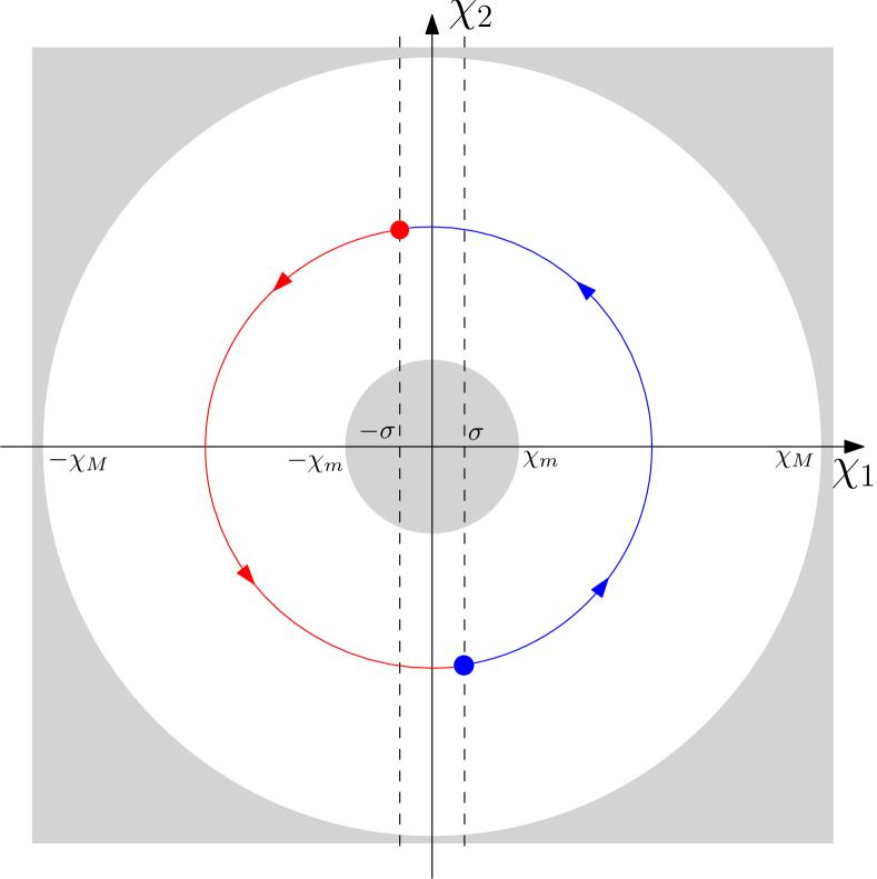
Figure 4: The white doughnut represents the set $\mathcal{W}$. The red/blue curve is a solution $\chi(t,j)$ where the dots represents jump instants. The solution is blue in regions where $\mathfrak{h}(\chi(t,j))=-1$ and is red in regions where $\mathfrak{h}(\chi(t,j))=1$

Adopting the notation introduced in the previous sections, define the functions $\mathfrak{h}:\mathbb{R}^{2}\rightarrow\{-1,1\}$ as

$$\mathfrak{h}(\chi):=\left\{\begin{array}[]{rcr}-1,&{\rm if}&\chi_{1}\geq\sigma\hskip 5.69046pt\lor\hskip 5.69046pt(|\chi_{1}|<\sigma\wedge\chi_{2}>0)\\ 1,&{\rm if}&\chi_{1}\leq-\sigma\hskip 5.69046pt\lor\hskip 5.69046pt(|\chi_{1}|<\sigma\wedge\chi_{2}<0)\end{array}\right.$$ (25)

and $\varrho:\mathbb{R}^{2}\times\mathbb{R}\rightarrow\mathbb{R}$ as $\varrho(\chi,\tau):=He^{S\left(\pi/\omega-\tau\right)}\chi-\mathfrak{h}(\chi)\sigma$, which is constant along flowing solutions because

$$\dot{\varrho}(\chi,\tau)=-He^{S\left(\pi/\omega-\tau\right)}S\chi+He^{S\left(\pi/\omega-\tau\right)}\dot{\chi}=0\,,$$ (26)

which is zero if and only if $\tau$ is suitably synchronized with $\chi$, namely such that $\tau^{+}=\pi/\omega$: this would in turn guarantee that $T^{+}=2\pi/\omega$ at the next jump provided that also $T=2\pi/\omega$. Then, consider the sets

$$\begin{split}\Gamma_{3}:=\Big{\{}\xi&\in\Xi:\varrho(\chi,\tau)=0\Big{\}}\,,\end{split}$$ (27)

$$\begin{split}\Gamma_{2}:=\Big{\{}\xi&\in\Gamma_{3}:T=\dfrac{2\pi}{\omega}\Big{\}}\end{split}$$ (28)

and

$$\begin{split}\Gamma_{1}:=\Big{\{}\xi&\in\Gamma_{2}:\chi=\hat{\chi}\Big{\}}\end{split}$$ (29)

with $\xi:=(\chi,\hat{\chi},q,T,\tau)$, which clearly satisfy $\Gamma_{1}\subset\Gamma_{2}\subset\Gamma_{3}$. Roughly speaking, on the set $\Gamma_{1}$ the state $\hat{\chi}$ of the hybrid estimator (21) is perfectly synchronized with that of system (20), $\Gamma_{2}$ consists of the set of states that ensure $T^{+}=2\pi/\omega$ at the next jump, while $\Gamma_{3}$ prescribes the correct value of the initial timer $\tau$, depending on the initial phase of $\chi$, such that at jumps $\tau$ coincides with $\pi/\omega$. Note that $\Gamma_{1}$ is compact, by the hypothesis on $\mathcal{W}$, while $\Gamma_{2}$ and $\Gamma_{3}$ are closed.

Let us now show GAS of $\Gamma_{1}$ by using reductions theorems. To this end, we apply the recursive version of Theorem IV.7 given in Theorem IV.9. In particular, we show GAS of $\Gamma_{1}$ relative to $\Gamma_{2}$, GAS of $\Gamma_{2}$ relative to $\Gamma_{3}$, GAS of $\Gamma_{3}$ and finally boundedness of solutions. To begin with, it can be shown that $\Gamma_{1}$ is globally asymptotically stable relative to $\Gamma_{2}$. In fact, letting $\eta_{1}=\chi-\hat{\chi}$ denote the estimation error, then its dynamics restricted to $\Gamma_{2}$, due to the trivial jumps of $\chi$ and $\hat{\chi}$, is described by the hybrid system defined by the flow dynamics

$$\dot{\eta}_{1}=S\chi-\hat{S}(T)\hat{\chi}-\hat{L}(T)H\eta_{1}=(S-\hat{L}(T)H)\eta_{1}\,,$$ (30)

which is obtained by considering that, on the set $\Gamma_{2}$, $\hat{S}(T)=S$, for $\xi\in\mathcal{C}$, and the jump dynamics $\eta_{1}^{+}=\eta_{1}$ for $\xi\in\mathcal{D}$. The claim follows by recalling that $\hat{L}(T)$ is such that $(S-\hat{L}(T)H)$ is Hurwitz and by persistent flowing conditions of stability [10, Proposition 3.27].

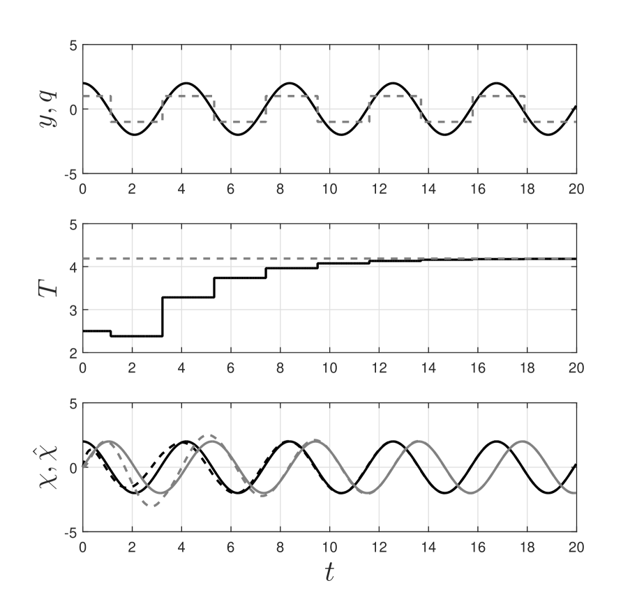
Figure 5: Top Graph: time histories of the function $y$ generated by (20) and of the state $q(t,k)$, solid and dashed lines, respectively. Middle Graph: time histories of the estimate $T(t,k)$, converging to the correct value of the period of oscillation $2\pi/\omega$. Bottom Graph: time histories of $\hat{\chi}_{1}(t,k)$ (dark) and $\hat{\chi}_{2}(t,k)$ (gray), solid lines, converging to the actual states $\chi_{1}(t,k)$ and $\chi_{2}(t,k)$, dashed lines.

Moreover, $\Gamma_{2}$ is globally asymptotically stable relative to $\Gamma_{3}$. To show this, let $\eta_{2}=T-2\pi/\omega$ and recall that all the trajectories of (21) that remain in $\Gamma_{3}$ are characterized by the property that $\tau=\pi/\omega$ at the time of jump. Therefore, the dynamics of $\eta_{2}$ restricted to $\Gamma_{3}$ is described by the hybrid system defined by the flow dynamics $\dot{\eta}_{2}=0$, for $\xi\in\mathcal{C}$ and the jump dynamics

$$\eta_{2}^{+}=T^{+}-\dfrac{2\pi}{\omega}=\lambda\left(T-\dfrac{2\pi}{\omega}\right)=\lambda\eta_{2}\,,$$ (31)

for $\xi\in\mathcal{D}$. Asymptotic stability of $\Gamma_{2}$ relative to $\Gamma_{3}$ then follows by persistent jumping stability conditions [10, Proposition 3.24], which applies because $\sigma>\chi_{m}$, and by recalling that $0\leq\lambda<1$. In addition, global attractivity of $\Gamma_{3}$ can be shown by relying on the fact that $\tau(t_{2},1)$, namely the value of $\tau$ before the second jump, is equal to $\pi/\omega$, hence implying that $\varrho(\chi(t,k),\tau(t,k))=0$ for $(t,k)\in{\rm dom}\,\varrho$ with $k>1$. Stability of $\Gamma_{3}$, on the other hand, follows by noting that a perturbation $\delta$ on $\tau(0,0)$ with respect to the values in $\Gamma_{3}$, $i.e.$ values that satisfy $\varrho(\chi,\tau)=0$, results in $\tau(t_{1},0)=\pi/\omega+\varepsilon(\delta)$, with $\varepsilon$ a class-$\mathcal{K}$ function of $\delta$.

Finally, boundedness of the trajectories of the state $\chi$ and of $q$, $T$ and $\tau$ follows by the existence of the strongly forward invariant set $\mathcal{W}$ - described by the lower, $\chi_{m}$, and upper, $\chi_{M}$, bounds - and by definition of the flow and jump sets, respectively. Therefore, to conclude global asymptotic stability of the set $\Gamma_{1}$ it only remains to show that the trajectories of $\hat{\chi}$ are bounded. Towards this end, recall the flow dynamics of $\hat{\chi}$ in (21), namely

$$\dot{\hat{\chi}}=(S(T)-\hat{L}(T)C_{o})\hat{\chi}+\hat{L}(T)C_{o}\chi:=M(T)\hat{\chi}+\hat{L}(T)C_{o}\chi\,,$$ (32)

with $M(T)$, and its derivative with respect to $T$, uniformly bounded in $T$, since $T\in[T_{m},T_{M}]$, and Hurwitz uniformly in $T$ by definition of $\hat{L}(T)$, whereas the jump dynamics is described by $\hat{\chi}^{+}=\hat{\chi}$. Thus, by applying [16, Lemma 5.12], it follows that there exists a unique positive definite solution $P(T)$ to the Lyapunov equation $P(T)M(T)+M(T)^{\top}P(T)=-I$, with the additional property that $c_{1}|\hat{\chi}|^{2}\leq\hat{\chi}^{\top}P(T)\hat{\chi}\leq c_{2}|\hat{\chi}|^{2}$, for some positive constants $c_{1}$ and $c_{2}$. Boundedness of the trajectories of $\hat{\chi}$ then follows by standard manipulations on the time derivative of the functions $\hat{\chi}^{\top}P(T)\hat{\chi}$ along the trajectories of (32) and by noting that $\hat{L}(T)$ is uniformly bounded, by the definition of $\hat{L}$ and of $T$, and by recalling that $|\chi|$ is uniformly bounded by definition of the strongly forward invariant compact set $\mathcal{W}$.

In the following numerical simulations, we suppose that $\omega=1.5$ and we let $\sigma=0.25$ and $\lambda=0.5$. Moreover, we let $\chi(0,0)=[2,\,0]^{\prime}$ and $\hat{\chi}(0,0)=[0,\,0]^{\prime}$, while the remaining components of the estimator are initialized as $q(0,0)=1$, $T(0,0)=2.5$ and $\tau(0,0)=0$. The top graph of Figure 5 depicts the time histories of the function $y$ generated by (20) and of the state $q(t,k)$, solid and dashed lines, respectively. The middle graph of Figure 5 shows the time histories of the estimate $T(t,k)$, converging to the correct value of the period of oscillation $2\pi/\omega$, while the bottom graph displays the time histories of $\hat{\chi}_{1}(t,k)$ (dark) and $\hat{\chi}_{2}(t,k)$ (gray), solid lines, converging to the actual states $\chi_{1}(t,k)$ and $\chi_{2}(t,k)$, dashed lines.

VI Conclusion

In this paper we presented three reduction theorems for stability, local/global attractivity, and local/global asymptotic stability of compact sets for hybrid dynamical systems, along with a number of their consequences. The proofs of these results rely crucially on the ${\cal KL}$ characterization of robustness of asymptotic stability of compact sets found in [10, Theorem 7.12]. A different proof technique is possible which generalizes the proofs found in [7]. As a future research direction, we conjecture that, similarly to what was done in [7] for continuous dynamical systems, it may be possible to state reduction theorems for hybrid systems in which the set $\Gamma_{1}$ is only assumed to be closed, not necessarily bounded.

In addition to the applications listed in the introduction, the reduction theorems presented in this paper may be employed to generalize the position control laws for VTOL vehicles presented in [24, 19], by replacing continuous attitude stabilizers with hybrid ones, such as the one found in [18]. Furthermore, the results of this paper may be used to generalize the allocation techniques of [22], possibly following similar ideas to those in [8].

References

- [1] A. Alessandri and L. Zaccarian, “Stubborn state observers for linear time-invariant systems,” Automatica, vol. 88, pp. 1–9, Feb. 2018.
- [2] A. Bisoffi, L. Zaccarian, M. D. Lio, D. Carnevale, and J. Contributors, “Hybrid cancellation of ripple disturbances arising in AC/DC converters,” Automatica., vol. 77, pp. 344–352, 2017.
- [3] C. Byrnes, A. Isidori, and J. Willems, “Passivity, feedback equivalence, and the global stabilization of nonlinear systems,” IEEE Transactions on Automatic Control, vol. 36, pp. 1228–1240, 1991.
- [4] M. El-Hawwary, “Passivity methods for the stabilization of closed sets in nonlinear control systems,” Ph.D. dissertation, University of Toronto, 2011.
- [5] M. El-Hawwary and M. Maggiore, “Reduction principles and the stabilization of closed sets for passive systems,” IEEE Transactions on Automatic Control, vol. 55, no. 4, pp. 982–987, 2010.
- [6] ——, “Distributed circular formation stabilization for dynamic unicycles,” IEEE Transactions on Automatic Control, vol. 58, no. 1, pp. 149–162, 2013.
- [7] ——, “Reduction theorems for stability of closed sets with application to backstepping control design,” Automatica, vol. 49, no. 1, pp. 214–222, 2013.
- [8] S. Galeani, A. Serrani, G. Varano, and L. Zaccarian, “On input allocation-based regulation for linear over-actuated systems,” Automatica, vol. 52, pp. 346–354, 2015.
- [9] R. Goebel, R. G. Sanfelice, and A. Teel, “Hybrid dynamical systems,” IEEE Control Systems, vol. 29, no. 2, pp. 28–93, 2009.
- [10] R. Goebel, R. Sanfelice, and A. Teel, Hybrid Dynamical Systems: modeling, stability, and robustness. Princeton University Press, 2012.
- [11] R. Goebel and A. Teel, “Solutions to hybrid inclusions via set and graphical convergence with stability theory applications,” Automatica, vol. 42, no. 4, pp. 573–587, 2006.
- [12] L. Greco, P. Mason, and M. Maggiore, “Circular path following for the spherical pendulum on a cart,” in IFAC World Congress, Toulouse, France, July 2017.
- [13] A. Iggidr, B. Kalitin, and R. Outbib, “Semidefinite Lyapunov functions stability and stabilization,” Mathematics of Control, Signals and Systems, vol. 9, pp. 95–106, 1996.
- [14] D. Invernizzi, M. Lovera, and L. Zaccarian, “Geometric tracking control of underactuated VTOL UAVs,” in American Control Conference, Milwaukee (WI), USA, Jul. 2018, pp. 3609–3614.
- [15] B. S. Kalitin, “B-stability and the Florio-Seibert problem,” Differential Equations, vol. 35, pp. 453–463, 1999.
- [16] H. Khalil, Nonlinear Systems, 2nd ed. USA: Prentice Hall, 1996.
- [17] M. Maggiore and L. Consolini, “Virtual holonomic constraints for Euler–Lagrange systems,” IEEE Transactions on Automatic Control, vol. 58, no. 4, pp. 1001–1008, 2013.
- [18] C. Mayhew, R. Sanfelice, and A. Teel, “Quaternion-based hybrid control for robust global attitude tracking,” IEEE Transactions on Automatic Control, vol. 56, no. 11, pp. 2555–2566, 2011.
- [19] G. Michieletto, A. Cenedese, L. Zaccarian, and A. Franchi, “Nonlinear control of multi-rotor aerial vehicles based on the zero-moment direction,” in IFAC World Congress, Toulouse, France, Jul. 2017, pp. 13 686–13 691.
- [20] A. Mohammadi, E. Rezapour, M. Maggiore, and K. Pettersen, “Maneuvering control of planar snake robots using virtual holonomic constraints,” IEEE Transactions on Control Systems Technology, vol. 24, no. 3, pp. 884–899, 2016.
- [21] C. Ott, A. Dietrich, and A. Albu-Schäffer, “Prioritized multi-task compliance control of redundant manipulators,” Automatica, vol. 53, pp. 416–423, 2015.
- [22] T. Passenbrunner, M. Sassano, and L. Zaccarian, “Optimality-based dynamic allocation with nonlinear first-order redundant actuators,” European Journal of Control, pp. 33–40, 2016.
- [23] F. Plestan, J. Grizzle, E. Westervelt, and G. Abba, “Stable walking of a 7-DOF biped robot,” IEEE Transactions on Robotics and Automation, vol. 19, no. 4, pp. 653–668, 2003.
- [24] A. Roza and M. Maggiore, “A class of position controllers for underactuated VTOL vehicles,” IEEE Transactions on Automatic Control, vol. 59, no. 9, pp. 2580–2585, 2014.
- [25] R. Sanfelice, R. Goebel, and A. Teel, “Invariance principles for hybrid systems with connections to detectability and asymptotic stability,” IEEE Transactions on Automatic Control, vol. 52, no. 12, pp. 2282–2297, 2007.
- [26] P. Seibert, “On stability relative to a set and to the whole space,” in Papers presented at the Int. Conf. on Nonlinear Oscillations (Izdat. Inst. Mat. Akad. Nauk. USSR, 1970), vol. 2, Kiev, 1969, pp. 448–457.
- [27] ——, “Relative stability and stability of closed sets,” in Sem. Diff. Equations and Dynam. Systs. II; Lect. Notes Math. Berlin-Heidelberg-New York: Springer-Verlag, 1970, vol. 144, pp. 185–189.
- [28] P. Seibert and J. S. Florio, “On the reduction to a subspace of stability properties of systems in metric spaces,” Annali di Matematica Pura ed Applicata, vol. CLXIX, pp. 291–320, 1995.
- [29] P. Seibert and R. Suárez, “Global stabilization of nonlinear cascaded systems,” Systems & Control Letters, vol. 14, no. 5, pp. 347–352, 1990.
- [30] E. Sontag, “Remarks on stabilization and input-to-state stability,” in Proc. of the IEEE Conference on decision and Control, Tampa, Florida, 1989, pp. 1376 – 1378.
- [31] A. Teel, “Observer-based hybrid feedback: a local separation principle,” in American Control Conference, Baltimore (MD), USA, June 2010, pp. 898–903.
- [32] J. Thunberg, J. Goncalves, and X. Hu, “Consensus and formation control on for switching topologies,” Automatica, vol. 66, pp. 109–121, 2016.
- [33] M. Vidyasagar, “Decomposition techniques for large-scale systems with nonadditive interactions: Stability and stabilizability,” IEEE Transactions on Automatic Control, vol. 25, no. 4, pp. 773–779, 1980.
- [34] E. Westervelt, J. Grizzle, C. Chevallereau, J. Choi, and B. Morris, Feedback control of dynamic bipedal robot locomotion. CRC press, 2007, vol. 28.
- [35] E. Westervelt, J. Grizzle, and D. Koditschek, “Hybrid zero dynamics of planar biped robots,” IEEE Transactions on Automatic Control, vol. 48, no. 1, pp. 42–56, 2003.