Dynamics of nanoscale bubbles growing in a tapered conduit

Abstract

We predict the dynamics and shapes of nanobubbles growing in a supersaturated solution confined within a tapered, Hele-Shaw device with a small opening angle $\Phi\ll 1$. Our study is inspired by experimental observations of the growth and translation of nanoscale bubbles, ranging in diameter from tens to hundreds of nanometers, carried out with liquid-cell transmission electron microscopy. In our experiments, the electron beam plays a dual role: it supersaturates the solution with gaseous radiolysis products, which lead to bubble nucleation and growth, and it provides a means to image the bubbles in-situ with nanoscale resolution. To understand our experimental data, we propose a migration mechanism, based on Blake-Haynes theory, which is applicable in the asymptotic limits of zero capillary and Bond numbers and high confinement. Consistent with experimental data, our model predicts that in the presence of confinement, growth rates are orders of magnitude slower compared to a bubble growing in the bulk and that the combination of a tapered channel and contact line pinning create tear-drop shaped bubbles.

I Introduction

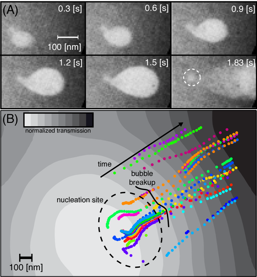
Figure 1: (A) A series of transmission electron microscopy images of a bubble growing under high, non-uniform confinement witinh a liquid cell, FIG. S1 and movie S1. The bubble formation occurred while imaging an aqueous solution of gold nanorods that contained a trace amount of the surfactant cetrimonium bromide (CTAB) with TEM at 300 keV, beam current $\sim$1−10 nA, and beam radius $\sim$2 $\mu$m. The bubble grows anisotropically and in the last frame detaches from the nucleation size (dashed white circle), the growth of this bubble is compared to theory in FIG. 8. (B) Normalized intensity (contours) with bubble trajectories (data points), nucleation site (dashed ellipse), and approximate location of bubble breakup (solid line).

The motion and shape of droplets and bubbles in confined geometries have attracted considerable attention in the scientific community due to their importance in industrial processes, multi-phase flows through porous media and recently, microfluidic devices. Typically at the macroscale, pressure driven flow or buoyancy drive motion of bubbles and fluid-fluid interfaces. G. I. Taylor and Saffman Saffman1958 ; Taylor1959 and Tanveer and Saffman Tanveer1987 studied the migration of droplets in Hele-Shaw cells. Matched asymptotic methods have subsequently been used to elucidate the geometry of gas bubbles in cylindrical tubes Bretherton1961 and in Hele-Shaw cells when the continuous phase either perfectly wets the surface Park1984 or when contact line dynamics are at play Weinstein1990 .

In the absence of applied pressure gradients and when drops are small such that the Bond number is much less than unity, gradients in substrate elasticity Style2012 ; Style2013 , chemistry Chaudhury1992 ; Darhuber2005 , temperature, and electric field, among others, can spontaneously drive the motion of contact lines and interfaces. Similarly, geometric gradients can induce capillary forces and promote transport of drops/bubbles confined in tapered capillaries Renvoise2009 and residing on wires with varying cross-sections Hanumanthu2006 ; Lorenceau2004 . To minimize their surface energy, wetting drops seek confinement while non-wetting drops and bubbles avoid it. The dynamics of bubbles and droplets in tapered Hele-Shaw devices have been modeled and compared to experiment Jenson2014 ; Metz2009 ; Reyssat2014 . In these cases a dynamically created film wets the substrate. Furthermore, the mass of the bubble or drop is fixed and so the process is purely relaxational. Droplets and bubbles begin in a non-equilibrium configuration and transport to their equilibrium positions, where they can exist as spheres (for completely wetting substrates) or spherical sections (for partially wetting substrates) that satisfy the equilibrium contact angle Langbein2002 . Laplace pressure gradients drive the disperse phase and hydrodynamics either in the bulk or at the contact line provide dissipation, setting the time scale for the process.

In recent years, there has been a considerable interest in surface-bound nanobubbles and their stability Alheshibri2016 ; Ball2012 ; Craig2011 ; Fang2016 . Understanding such bubbles has the potential to improve processes such as acoustic surface scrubbing Liu2008 ; Liu2009 ; Yang2011 and designing surface textures that optimize onset of nucleate boiling to enhance heat transfer Dong2014 ; Fazeli2015 ; Chu2012 . Free nano-bubbles can also be used as contrast agents in ultra-sonic imaging Cai2015 and so developing processes which reliably produce nanobubles could have applications in medical imaging as well. Due to the extremely high Laplace pressure of free bubbles, mass transfer-driven dissolution can dominate dynamics when the bubbles are below their critical radius. As the radius of curvature increases $R^{-1}$, the internal pressure $P$ and the equilibrium surface concentration $C_{\text{s}}$ rise; the latter in accordance with Henry’s law, $C_{\text{s}}\propto P\propto R^{-1}$. This positive feedback results in rapid dissolution; a bubble 100nm in radius will dissolve in $\sim$100$\mu$s Epstein1950 ; Ljunggren1997 . In contrast to the above prediction, surface-bound nanobubbles have been observed to persist for many hours Zhang2008 ; Seddon2011 ; Sun2016 . Researchers have proposed various mechanisms for this anomalous behavior, including a perpetual dynamic equilibrium Petsev2013 ; Seddon2011 , the stabilizing effect of organic contaminants Zhang2012 , and contact line pinning Weijs2013 ; Lohse2015 ; Maheshwari2016 . The constraint of a pinned contact line introduces a negative feedback by forcing the radius of curvature to decrease as the mass of the bubble decreases. As the surface concentration of dissolved gases decreases and approaches that of the bulk concentration, mass transfer slows.

Inspired by this simple feedback mechanism between the geometry of a bubble and its growth, we reaxmine the transport of bubbles in tapered Hele-Shaw cells when mass transfer and contact line dynamics dominate the system behavior. We develop our model around experimental observations of nanobubbles $R\sim 10-100$nm growing and migrating in tapered Hele-Shaw cells with plate gaps $\sim$10-100s of nanometers, FIG. 1Grogan2014 . The bubbles grow anomalously slow when compared to classical mass transfer limited growth theories Epstein1950 and despite their small size and velocities (the capillary numbers are in the range $10^{-9}-10^{-7}$ and Bond numbers $10^{-11}-10^{-9}$) are rarely spherical in shape. To explain both observations, we posit that the contact line is slow to relax compared to the rate of mass transfer and dominates bubble shape, growth rate, and translation in a regime where the gas-liquid interface is always at mechanical equilibrium (uniform Laplace pressure). We utilize the Blake-Haynes (BH) mechanism to model contact line movement. When a portion of the contact line is immobilized, a teardrop shaped bubbles result, similar to those observed in our experiments.

II Bubble Growth and Migration Model

Our goal is to model contact line evolution of a bubble growing in a supersaturated solution confined between two plates diverging at an $2\Phi$. FIG. 2A depicts top view of the bubble. The bubble is symmetric with respect to the $x$-axis. The inner contour (solid line) is the projection of the bubble’s contact line with the confining plates onto the $xy$-plane and is defined with the polar coordinate $\rho\left(\psi,t\right)$, where $\psi$ is the azimuthal angle and $t$ is time. The intersection of the bubble’s surface with the $xy$-plane is shown as the outer, dashed contour. FIG. 2B depicts the cross-section of the bubble confined in the tapered conduit. The two plates are distance $2h\left(\mathbf{x},t\right)$ apart. We restrict our analysis to cases when $R\left(t\right)\ll\min\limits_{\psi}\rho\left(\psi,t\right)$. In the limit of zero capillary and Bond numbers, the pressure inside the bubble is nearly uniform and dominated by the smallest radius of curvature $R$. Hence, we take $R$ to be $\psi$-independent. $\theta\left(\psi\right)$ is the dynamic contact angle between the continuous phase (liquid) and the plates. The contact angle may vary as a function of position.

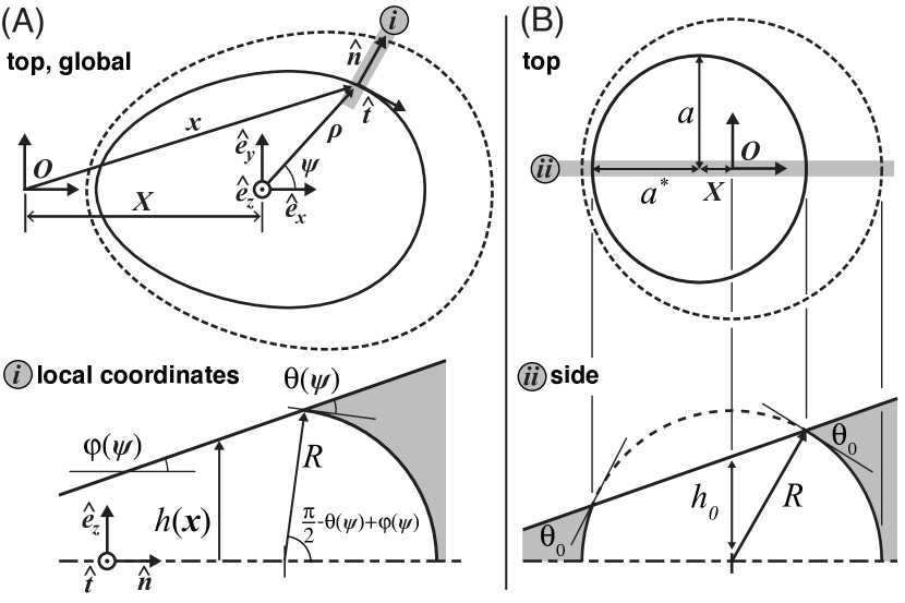
Figure 2: : (A) Schematic of the geometry of our problem with global perspectives of a bubble shape (top) as seen from the top and a cross section of the interface as viewed from the local coördinate system (i); the unit vectors of the latter are defined by the local tangent and normal vectors of the bubble’s interface at the $xy$-plane; both the slope $\varphi$ and contact angle $\theta$ are local properties and depend on the polar angle $\psi$. (B) Top and cross-section (through the plane ii) view of the initial condition used for the model, a sphere with a circular contact line that when projected onto the $xy$-plane is an ellipse with major and minor radii $\{a,a^{*}\}$.

The projection of a contact line point on the $x-y$ plane is given by the two-dimensional vector

$${\bf{x}}\left({\psi,t}\right)=\left\{{\rho\left({\psi,t}\right)\cos\psi+X\left(t\right),\rho\left({\psi,t}\right)\sin\psi}\right\}.$$ (1)

In the above, $X$ is the distance of the origin of $\rho$ from the center of the initial $\left(t=0\right)$ bubble geometry, which we will later define to be a sphere (eqn. 22). $2h_{0}$ is the height of the conduit at $X=0$.

We define local planar coordinates aligned with the normal $\hat{\mathbf{n}}$ and tangent $\hat{\mathbf{t}}$ to the projection of the contact line on the $xy$-plane. Using FIG. 2i as a guide, we relate the radius of curvature $R$ to the slope of the wedge, contact angle, and channel height at the contact line in the plane that is both normal to the contact line at position $\mathbf{x}$ and the $xy$- plane.

$$h=R\cos\left({\theta\left(\psi\right)-\varphi\left(\psi\right)}\right).$$ (2)

Additionally,

$$h={h_{0}}+x\tan\Phi={h_{0}}+\left({X+\rho\cos\psi}\right)\tan\Phi.$$ (3)

Equating eqn. 2 and 3 and solving for the contact angle $\theta$ gives

$$\theta={\cos^{-1}}\left[{\frac{{{h_{0}}+\left({X+\rho\cos\psi}\right)\tan\Phi}}{R}}\right]+\varphi.$$ (4)

The local wedge angle $\varphi\left(\theta\right)$ relates to the global or maximum wedge angle $\Phi$ through

$$\tan\varphi={\bf{\hat{n}}}\cdot{{\bf{\hat{e}}}_{x}}\tan\Phi$$ (5)

When ${\left.{{\bf{\hat{n}}}}\right|_{\psi=0}}={{\bf{\hat{e}}}_{x}}$ eqn. 5 yields ${\left.\varphi\right|_{\psi=0}}=\Phi$; when ${\left.{{\bf{\hat{n}}}}\right|_{\psi=\pi/2}}={{\bf{\hat{e}}}_{y}}$ , ${\left.\varphi\right|_{\psi=\pi/2}}=0$. In radial coordinates, the normal vector to the contact line curve

$${\bf{\hat{n}}}=\left\{{\begin{array}[]{*{20}{c}}{\rho\cos\psi+\frac{{\partial\rho}}{{\partial\psi}}\sin\psi}\\ {\rho\sin\psi-\frac{{\partial\rho}}{{\partial\psi}}\cos\psi}\end{array}}\right\}\mathcal{N}^{-1},$$ (6)

where $\mathcal{N}=\sqrt{{\rho^{2}}+{{\left({{\partial\rho}/{{\partial\psi}}}\right)}^{2}}}$, which follows from ${\bf{\hat{n}}}={{\frac{{d{\bf{\hat{t}}}}}{{d\psi}}}\mathord{\left/{\vphantom{{\frac{{d{\bf{\hat{t}}}}}{{d\psi}}}{\left|{\frac{{d{\bf{\hat{t}}}}}{{d\psi}}}\right|}}}\right.\kern-1.2pt}{\left|{\frac{{d{\bf{\hat{t}}}}}{{d\psi}}}\right|}}$, where ${\bf{\hat{t}}}={{\frac{{d{\bf{x}}}}{{d\psi}}}\mathord{\left/{\vphantom{{\frac{{d{\bf{x}}}}{{d\psi}}}{\left|{\frac{{d{\bf{x}}}}{{d\psi}}}\right|}}}\right.\kern-1.2pt}{\left|{\frac{{d{\bf{x}}}}{{d\psi}}}\right|}}$ is the unit tangent vector. The full equation for the local inclination angle

$$\varphi=\tan^{-1}\left[{\tan\Phi}\left({\rho\cos\psi+\frac{{\partial\rho}}{{\partial\psi}}\sin\psi}\right)\mathcal{N}^{-1}\right].$$ (7)

The full expression for the local contact angle is therefore given by substituting eqn. 7 into eqn. 4. The projection of the linearized Blake-Haynes (BH) velocity Blake1969 ; Blake2006 for contact line motion onto the $x-y$ plane gives the normal velocity of the interface

$$\frac{{\partial{\mathbf{x}}}}{{\partial t}}\cdot{\bf{\hat{n}}}={U_{0}}\cos\varphi\left({\cos\theta-\cos{\theta_{0}}}\right),$$ (8)

where

$$\frac{{\partial{\mathbf{x}}}}{{\partial t}}=\left\{{\frac{{dX}}{{dt}}+\frac{{\partial\rho}}{{\partial t}}\cos\psi,\frac{{\partial\rho}}{{\partial t}}\sin\psi}\right\}.$$ (9)

$U_{0}=\gamma/\eta_{\text{CL}}$ is the contact line’s velocity scale defined in terms of the contact line viscosity $\eta_{\text{CL}}$ and the surface tension of the gas-liquid interface $\gamma$. We assume that the continuous phase (water) only partially wets the solid substrate (silicon nitride) ($\theta_{0}>0$). Previously, the BH equation has been successfully applied to model the adsorption dynamics of colloids at interfaces Kaz2012 . Since the observed interfacial velocities in our experiments are well below the threshold required to support a dynamically-formed liquid film Brochard-Wyart2001 , we assume that the gaseous phase contacts the solid surfaces at all times. In the supplement, we compare bulk and contact line hydrodynamic dissipation with that of BH wetting/de-wetting and determine that the latter dominates the system. Although the disjoining pressure may influence the details of the interface geometry and play a role in wetting and de-wetting dynamics when the gap between the plates is small, this effect is not accounted for by the coarse-grain BH model.

Substititung eqns. 4 and 7 into eqn. 9 and linearizing for $\Phi\ll 1$ and $\partial\rho/\partial\psi\ll 1$ about $\Phi=0$ and $\partial\rho/\partial\psi=0$, we obtain

$$\frac{{\partial\rho}}{{\partial t}}+\frac{{dX}}{{dt}}\left({\frac{{\sin\psi}}{\rho}\frac{{\partial\rho}}{{\partial\psi}}+\cos\psi}\right)+\mathcal{O}\left(\left({{{\frac{{\partial\rho}}{{\partial\psi}}}}}\right)^{2}\right)=\\ U_{0}\left\{\frac{h_{0}}{R}+\Phi\left[\frac{X}{R}+\cos\psi\left(\frac{\rho}{R}-H\right)-\frac{\sin\psi H}{\rho}\frac{\partial\rho}{\partial\psi}\right.\right.\\ \left.\left.+\mathcal{O}\left(\left(\frac{\partial\rho}{\partial\psi}\right)^{2}\right)\right]-\cos\theta_{0}+\mathcal{O}\left(\Phi^{2}\right)\right\}$$ (10)

where $H=\sqrt{1-\left(h_{0}/R\right)^{2}}$.

In our experiments, we observed bubbles with an advancing front and a pinned aft, FIG. 1. To accommodate such situations, we modified the BH theory, introducing the weighing pre-factor $\left(1+\cos\psi\right)/2$ such that eqn. 10 becomes

$$\frac{{\partial\rho}}{{\partial t}}+\frac{{dX}}{{dt}}\left({\frac{{\sin\psi}}{\rho}\frac{{\partial\rho}}{{\partial\psi}}+\cos\psi}\right)=\\ U_{0}\frac{\left(1+\cos\psi\right)}{2}\left\{\frac{h_{0}}{R}+\Phi\left[\frac{X}{R}+\cos\psi\left(\frac{\rho}{R}-H\right)\right.\right.\\ \left.\left.-\frac{\sin\psi H}{\rho}\frac{\partial\rho}{\partial\psi}\right]-\cos\theta_{0}\right\}$$ (11)

The above weighting function smoothly reduces the contact line velocity from its maximum value at $\psi=0$ to zero at $\psi=\pi$ .

In defining our coordinate system, we introduced the variable $X$, denoting the position of the bubble’s center, without providing a rigorous definition. We do so now by selecting $X\left(t\right)$ such that $\rho\left(0,t\right)=\rho\left(\pi,t\right)$ at all times. Equivalently, $\left.\partial\rho/\partial t\right|_{\psi=\pi}=\left.\partial\rho/\partial t\right|_{\psi=0}$ with $\rho\left(0,0\right)=\rho\left(\pi,0\right)$. Evaluating eqn. 10 for $\psi=0$ and $\psi=\pi$, subtracting the results, and incorporating $\left(\partial\rho/\partial t\right)|_{\psi=\pi}=\left(\partial\rho/\partial t\right)|_{\psi=0}$ we obtain the evolution equation for $X$ for the unpinned case

$$2R\left(\frac{dX}{dt}+{U_{0}}\Phi H\right)={U_{0}}\Phi\left({\rho\left({0,t}\right)+\rho\left({\pi,t}\right)}\right)$$ (12)

Following the same procedure but with eqn. 11 gives the evolution for $X$ for the pinned case

$$R\left(2\frac{dX}{dt}+U_{0}\Phi H\right)=\\ U_{0}\left\{\left[h_{0}+\Phi\left(X+\rho\left(0,t\right)\right)\right]-R\cos\theta_{0}\right\}$$ (13)

The evolution of the unpinned contactline is governed by eqns. 10 and 12; the pinned contactline is governed by 11 and 13. To complete our model, we still need to address the dependence of $R$ on time. For example, in an isobaric process, one would expect $\dot{R}=0$. In the supplement, we consider a Gedanken experiment, wherein the bubble’s volume is controlled in a specific way $V\propto t^{3}$. Although perhaps not practical, this case is instructive as it admits geometrically self-similar growth in the asymptotic limit $t\rightarrow\infty$, which is helpful for understanding contact line dynamics when the growth rate is independent of $R$. Here, however, we are interested in mass transfer-driven growth, which we address below.

We begin by writing an expression for the volume of the bubble; it can be divided into two contributions, a nearly cylindrical portion

$${V_{\text{I}}}=\int\limits_{0}^{2\pi}{{\rho^{2}}\left({{h_{0}}+\rho\cos\psi{\mathop{\rm tan}\nolimits}\Phi}\right){\rm{d}}\psi}$$ (14)

and the portion that bulges out from the contact line

$${V_{\text{II}}}=\int\limits_{0}^{2\pi}{\frac{{{R^{2}}}}{2}\left(\begin{array}[]{l}\pi-2\theta+2\varphi\\ -\sin\left({2\theta-2\varphi}\right)\end{array}\right){\cal N}{\rm{d}}\psi}$$ (15)

In eqn. 15, we assumed $R/\rho\ll 1$ to simplify the integrand. The integrals can be further simplified by applying, as before, the linearization, $\Phi\ll 1$ and $\partial\rho/\partial\psi\ll 1$, to yield

$$V=V_{\text{I}}+V_{\text{II}}=\\ \int\limits_{0}^{2\pi}{\frac{1}{2}\rho\left\{{2{h_{0}}\rho+{R^{2}}\left[{\pi-2{{{\mathop{\rm cos}\nolimits}}^{-1}}\left({\frac{{{h_{0}}}}{R}}\right)-\sin\left({2{{{\mathop{\rm sin}\nolimits}}^{-1}}\left({\frac{{{h_{0}}}}{R}}\right)}\right)}\right]}\right\}}\\ +\Phi\left[\frac{2}{3}{\rho^{3}}\cos\psi-h_{0}^{2}\frac{{\partial\rho}}{{\partial\psi}}\sin\psi+{\rho^{2}}\left({\frac{{2h_{0}^{2}\cos\psi}}{{RH}}+X}\right)\right.\\ \left.+\rho h_{0}^{2}\left({\cos\psi+\frac{{2X}}{{RH}}}\right)\right]+\mathcal{O}\left({{\Phi^{2}}}\right)\mathcal{O}\left({{{\frac{{\partial\rho}}{{\partial\psi}}}^{2}}}\right){\rm{d}}\psi$$ (16)

Next, we derive the expression for the effective surface area of a bubble available for mass transport. While the bubble is not perfectly cylindrical, the radius of the outward bulge is small compared to the overall radius of the contact line. We therefore expect the concentration field around the bubble to be essentially similar to that around a cylindrical bubble. Hence, the surface area

$$S\sim\int\limits_{0}^{2\pi}{\int\limits_{-h\left(\rho\right)}^{h\left(\rho\right)}\mathcal{N}{\rm{d}}z{\rm{d}}\psi}.$$ (17)

Integration in the $z$-direction gives

$$S=2\int\limits_{0}^{2\pi}{\left({{h_{0}}+\left({X+\rho\cos\psi}\right){\mathop{\rm tan}\nolimits}\Phi}\right)\mathcal{N}}{\rm{d}}\psi$$ (18)

and linearizing yields

$$S=2\int\limits_{0}^{2\pi}{\rho\left({{h_{0}}+\Phi\left({X+\rho\cos\psi}\right)}\right)+\mathcal{O}\left({{\Phi^{2}}}\right)\mathcal{O}{{\left({\frac{{\partial\rho}}{{\partial\psi}}}\right)}^{2}}{\rm{d}}\psi}.$$ (19)

Next, we estimate the quasi-static total mass flux $\dot{n}$ into a bubble growing in a supersaturated solution with fixed far field concentration $C_{\infty}$ (at $\rho=\rho_{\infty}$) by solving the steady diffusion equation in cylindrical coordinates. We assume that the bubble’s contact line is nearly circular with radius $\rho\sim\rho_{0}$ (where $\rho_{0}$ is the leading order coefficient describing the shape of the contact line and will be described in eqn. 26). The gas concentration next to the bubble’s surface $C_{s}=C\left(\rho=\rho_{0}\right)$ is given by a combination of Laplace’s equation and Henry’s law $C_{s}=K\left(P_{\infty}+\gamma/R\right)$, where $K$ is the Henry constant. In the above, we again took advantage of $R/\rho\ll 1$ by assuming that only the confinement radius $R$ contributes to the Laplace pressure. For simplicity, we assume that the state of the gas inside the bubble is described with the ideal gas equation of state $PV=nBT$, where $P$ is the pressure, $B$ is the universal gas constant, and $T$ is the absolute temperature. Taking the time derivative of the state equation and using eqns. 16 and 19 gives the differential equation that couples geometry and pressure (radius of curvature)

$$\left({{P_{\infty}}+\frac{\gamma}{R}}\right)\dot{V}-\gamma V\frac{{\dot{R}}}{{{R^{2}}}}=\\ S\frac{{D\left[{{C_{\infty}}-K\left({{P_{\infty}}+\gamma/R}\right)}\right]}}{{\ln\left({{\rho_{0}}/{\rho_{\infty}}}\right)}}BT$$ (20)

We define supersaturation $\alpha$ or the excess dissolved gas concentration relative to the surface concentration of the initial bubble

$$\alpha={\log_{10}}\left(C_{\infty}/C_{0}-1\right),$$ (21)

where ${C_{0}}=K\left({{P_{\infty}}+\gamma/R\left({t=0}\right)}\right)$. When supersaturation is large, the system is driven at a rate that is incommensurate with the BH velocity and the contact angle goes to zero somewhere along the contact line. To avoid such a situation, we restrict our analysis to small and moderate supersaturations.

For concreteness, we consider here circumstances when the initial geometry of the bubble is a spherical section with equilibrium contact angle along the entire contact line. While a spherical bubble does not satisfy our assumption $R/\rho\ll 1$, it is the only geometry that creates a uniform contact angle along the entire contact line. Any other geometry would introduce additional dynamics at early times, which we wish to avoid. While this initial state is somewhat artificial, we find that, in practice, the condition $R/\rho\ll 1$ is reached quickly. FIG. 2B depicts the geometry of the initial state of our bubble. Based on simple geometric considerations, we have the following relationship between the initial radius and the height of the channel at the center of the sphere

$$R_{0}=R\left(t=0\right)=h_{0}\frac{\cos\Phi}{\cos\theta_{0}},$$ (22)

where $h_{0}$ is used in the definition of our coordinate system eqn. 3. The initial contact line shape is a circle with radius $R_{0}\sin\theta_{0}$. The projection of this circle onto the $x-y$ plane is an ellipse with major and minor radii $\left\{a,a^{*}\right\}$ given by

$$\left\{{\begin{array}[]{*{20}{c}}a\\ a^{*}\end{array}}\right\}=\left\{{\begin{array}[]{*{20}{c}}{{{R}_{0}}\sin{\theta_{0}}}\\ {{{R}_{0}}\sin{\theta_{0}}\cos\Phi}\end{array}}\right\}=\left\{{\begin{array}[]{*{20}{c}}{{h_{0}}\tan{\theta_{0}}\cos\Phi}\\ {{h_{0}}\tan{\theta_{0}}{{\cos}^{2}}\Phi}\end{array}}\right\}$$ (23)

In our polar coordinate system centered about $X$, the contact line is described by

$$\rho\left(\psi,{t=0}\right)=\frac{{{h_{0}}\tan{\theta_{0}}{{\cos}^{2}}\Phi}}{{\sqrt{{{\cos}^{2}}\psi+{{\cos}^{2}}\Phi{{\sin}^{2}}\psi}}}$$ (24)

where the initial center of the bubble

$$X\left({t=0}\right)=-{h_{0}}\sin\Phi\cos\Phi.$$ (25)

As illustrated by FIG. 2B, $X\left(t=0\right)$ is negative because the center of the initial contact line is to the left of the center of the initial sphere, which serves as the origin of the global coordinate system. To summarize, the problem statement consists of a partial differential equation (the BH relationship for contact line velocity for unpinned eqn. 10 and pinned cases eqn. 11 ), equation of state eqn. 20, evolution equation for the bubble’s center (unpinned eqn. 12 and pinned eqn. 13), and initial conditions (eqns. 24 and 25).

To simplify the numerical solution of this hybrid system of equations, we assume that $\rho$ is a continuous function of $\psi$ and use a spectral decomposition of the contact line’s position

$$\rho\left({\psi,t}\right)=\sum\limits_{n=0}^{N}{{\rho_{n}}\left(t\right)\cos\left({n\psi}\right)}.$$ (26)

Only cosine terms are used in the above expansion because we restrict our analysis to bubbles symmetric with respect to the principal axis of the wedge $\psi=0,\pi$). We substitute eqn. 26 into the BH equation (eqns. 10 or 11) and require that it is satisfied in the sense of the weighted residuals

$$\int\limits_{0}^{2\pi}{\cos\left({n\psi}\right)\left({\text{BH}_{\text{LHS}}-\text{BH}_{\text{RHS}}}\right){\rm{d}}}\psi=0,{\rm{}}n=0,1,2\cdots.$$ (27)

We show terms for the case $N=2$ in the electronic supplement. The above decomposition has the virtue of not only reducing the system to a set of non-linear ordinary differential equations, but also readily incorporating integral (eqn. 20) and evolution equations (eqn. 12 or eqn. 13) in the model. We find rapid convergence and very few modes are needed when no-pinning is used (i.e. when bubbles are free to translate, the contact line is nearly circular at all times). In the presence of pinning, the model with $N=$5 functions well for moderate time and is able to model bubble growth to the point they detached in the experiment. For long times, higher frequency modes begin to dominate, which invalidates assumptions made in our model. While we only use cosine terms, the problem could be generalized to include sine terms if, for example, initial conditions with broken symmetry were of interest or if one wished to include additional forces acting transverse to the wedge axis; otherwise, there is no physical reason for information to flow into the odd functions given the problem’s symmetry.

III Experimental Method and Observations

We imaged bubble nucleation, growth, and migration in our custom-made liquid cell (the nanoaquarium) Grogan2010 ; Grogan:2011dj ; Grogan2014 with a transmission electron microscope (TEM). The liquid cell consists of a thin (nominally 200 nm) liquid layer confined and hermetically sealed between two very thin (50nm) silicon nitride membranes (100 $\mu$m x 100 $\mu$m). See FIG. S1 in the electronic supplement for a schematic depiction of our liquid cell. Additional details on the structure of the liquid cell and its fabrication are available in Grogan and Bau Grogan2010 . The liquid is sealed from the vacuum of the electron microscope and the entire assembly is thin enough to be transparent to electrons. In our experiments, the liquid cell is filled with a solution of water with trace amount of the surfactant cetrimonium bromide (CTAB). The liquid cell is imaged at 300kV using a beam of diameter 4 $\mu$m and current 1nA. FIG. 1 (movie S1) shows a series of bubbles nucleating from a location that is most likely a defect such as a pit on the interior surface of one of the liquid cell windows. These bubbles form because of radiolysis of water by the electron beam that generates gaseous species. The primary species are hydrogen and oxygen Schneider2014 , their production induces bubble nucleation and sustains bubble growth. Liquid cell electron microscopy is a new that can provide nanometer resolution of aqueous samples Ross2015 . In terms of imaging fluid dynamics phenomena, the technique is still evolving: the liquid layer geometry can not be defined accurately by the microscopist and the nucleation sites for bubbles are determined by random defects in the silicon nitride windows. This restricts our observations to somewhat uncontrolled experiments and precludes quantitative comparison between our theoretical predictions and data. Nevertheless, the liquid cell provides sufficient information to allow us to qualitatively compare our theoretical predictions with experimental data. TEM liquid cell microscopy has been used previously to image condensation Bhattacharya:2014cr , motion of droplets Mirsaidov2012a , dewetting phenomena Mirsaidov2012b and bubble formation by heating White2012 however, the physics behind these phenomena have not been modeled extensively and appear distinct from the phenomena discussed here.

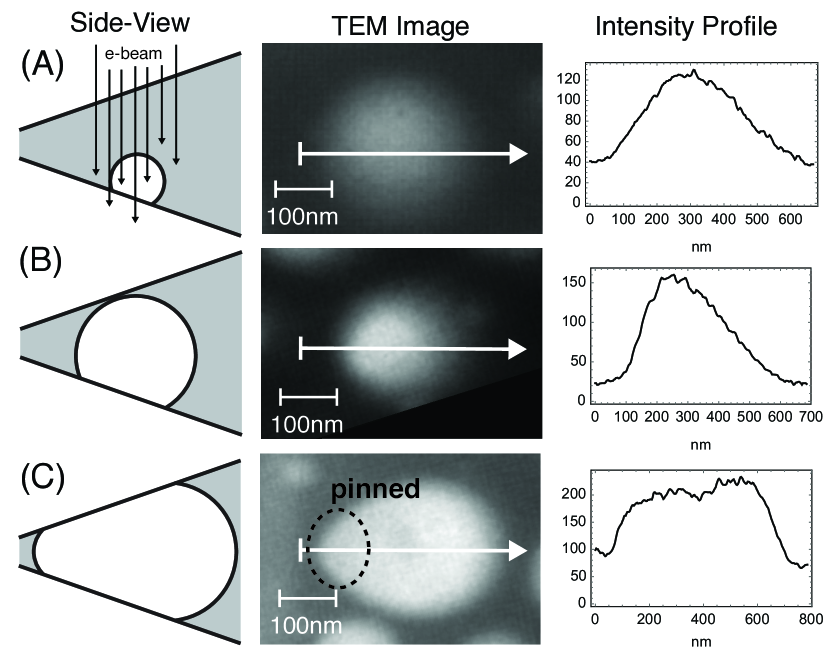
Figure 3: (A-C) A series of schematics (1st column), bright field electron micrographs (2nd column) and intensity profiles taken alone the midline of the bubble indicated on the images (3rd column) of a bubbles growing in under confinement. The bubble in (C) is pinned to a nucleation site.

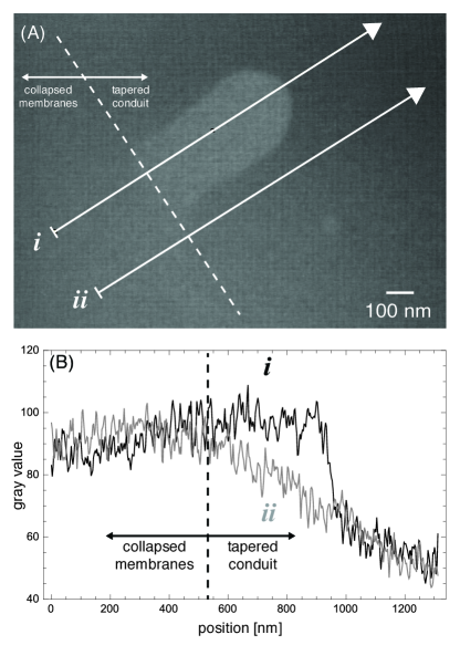
Figure 4: (A) and (B), respectively, show a microscopy image and corresponding intensity profiles ( i is taken along the centerline of the bubble, while ii is taken parallel to it in a nearby region of the device ). Since the transmission of (ii) is flat and similar to that of the bubble (i) we conclude that the membranes have contacted, along the line labled in (A) and (B).

FIG. 3A-C shows bright field electron microscope images of bubbles growing under confinement in our liquid cell. Three bubbles at different stages in their growth are shown along with a schematic side view (first column) that interprets the intensity profiles (third column). The scatter of electrons by the irradiated medium and the darkness of the image scale with the integrated atomic number density along the beam’s path, or in our case, the local thickness of water. Darker (lower intensity) sections of the image therefore indicate a thicker liquid layer. The flat intensity profile of the bubble FIG. 3C indicates that the bubble has contacted both membranes, while the “shaded” bubbles in (A) and (B) indicate that electrons encounter both liquid and vapor along their path and that the bubbles have therefore not contacted both surfaces.

When we observe nucleation, the bubbles appear to emanate periodically from a presumed impurity in the silicon nitride film. FIG. 1 shows snapshots of bright field electron microscope micrographs of a bubble growing under high confinement (movie S1). We compare our theory to bubbles like these. Nucleated bubbles are first observed when they are $\sim 80$ nm in diameter and depart when they are $\sim 250$nm in size. The bubbles depart by breaking into two bubbles: a smaller bubble that remains attached to the nucleation site and a larger bubble that continues to translate. The process repeats with a frequency of 0.3 Hz. The reproducibility of the process from one bubble to the next suggests quasi-static far field supersaturation Grogan2014 . Indeed, theory suggests that the radiolysis process is self-regulating and that the concentration of radiolysis products achieve steady state Schneider2014 . Since we cannot measure the dissolved gas concentration, we use it as a fitting parameter in our model, $\alpha$ eqn. 21.

The experimental data suggests that locally, bubbles always migrate in the same direction towards lower confinement, FIG. 1B. In support of this, we show a bubble at a different nucleation site FIG. 4A; FIG. 4B depicts two intensity profiles along parallel lines (i) and (ii), shown as arrows in FIG. 4A. Profile (i) includes the bubble and profile ii goes alongside the bubble. The recorded intensity declines as we go from left to right along the line (ii), suggesting that the thickness of the liquid layer increases from left to right. Furthermore, the similar transmitted intensity of the bubble compared to the region from which it emanates indicate a very thin liquid layer and possibly membrane contact. During loading of the liquid cell, capillary forces can pull the silicon nitride membranes into close proximity. We show such collapsed membranes in the supplement at lower magnification using optical microscopy (FIG. S2). FIG. 4 and FIG. S3 show that bubbles grow and migrate in the tapered conduit in the direction of diverging plates. This is the situation for which we built our model in Section II above. Like FIG. 3C, the detected intensity along the bubble (i) is nearly uniform and the transition from the bubble to the bulk liquid is relatively rapid compared to the size of the bubble’s plateau, one can infer that the bubble is highly confined, justifying the assumption made in the theory section $R/\rho\ll 1$.

Using simple image processing algorithms, we automate measurements of bubble features such as centroid position, area, and contact line shape and stitch together bubble trajectories using established techniques Schneider:2016hm ; Blair . In the Section V, we compare experimental observations with theoretical predictions.

IV Model Results and Discussion

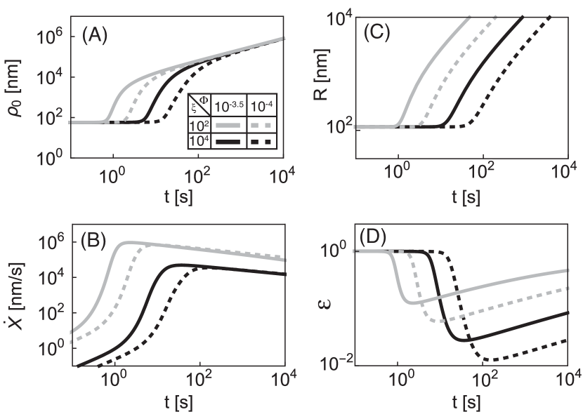
Figure 5: Model predictions for (A) bubble size, (B) velocity and (C) radius of curvature and (D) aspect ratio for two different slopes and contact line viscosities: $\xi=10^{2}$ (gray) and $\xi=10^{4}$(black), and slopes $\Phi=10^{-4}$ (dotted) and $\Phi=10^{-3.5}$ (solid) . In all cases $h_{0}=100$ nm and $\alpha=-6$.

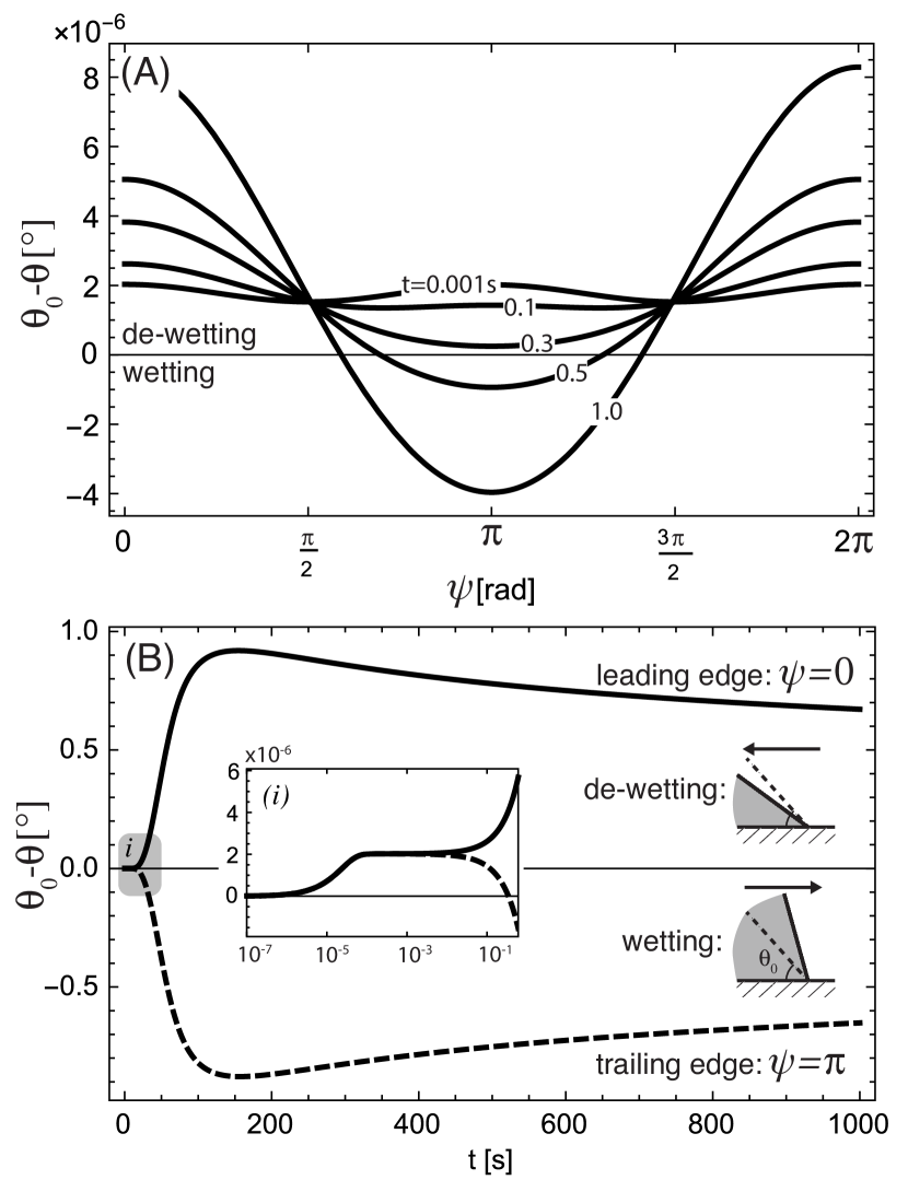
Figure 6: (A) Contact angle $\theta\left(\psi,t\right)$ relative to the equilibrium contact angle $\theta_{0}$ as a function of polar angle $\psi$ at a few different stages in bubble growth. (B) $\theta_{0}-\theta$ at the leading (solid) and trailing (dashed) edges of the bubble as a function of time; for $t>0.3$ s dewetting occurs at the leading edge and wetting occurs at the trailing edge. Inset (i) shows short dynamics in which, the bubble expands in all directions. $h_{0}=100$nm, $\alpha=-6$, $\xi=10^{4}$, and $\Phi=10^{-4}$.

In all our theoretical predictions, we assume that the gaseous species is hydrogen and that the liquid cell is at room temperature ( $T=298$ K) and pressure ( $P=0.1$ MPa) Grogan2014 . We assume that as bubbles grow they do not significantly increase the pressure of the device since their volume is miniscule to that of the device. We use $\theta_{0}=30^{\circ}$ Arkles2006 , $K_{\text{H}_{2}}=7.74\times 10^{-6}$ mol/Pa $\text{m}^{3}$ Sander2015 , $D_{\text{H}_{2}}$ $\text{m}^{2}$/s Cussler2009 , $\eta_{\text{CL}}=k_{\text{B}}T/\left(\kappa_{0}\lambda^{3}\right)=\xi\eta_{0}$ Pa s Petrov1997 ; Blake2006 , bulk viscosity $\eta_{0}=8.9\times 10^{-4}$ Pa s, and surface tension of the vapor-liquid interface and $\gamma=40$ mN/m. We use surface tension of the gas-liquid interface lower than that of pure water to account for the presence of trace amounts of the CTAB surfactant in our experiment Berg2010 . The negative value for $\alpha$ corresponds to a far field gas concentration that is only slightly above the equilibrium concentration at the surface of the initial bubble. In the expression for the contact line viscosity $\lambda$ is the lattice spacing, $k_{\text{B}}$ is the Boltzman constant, and $\kappa_{0}$ is the hopping frequency. We explore a range of dimensionless contact line viscosities ($\xi=\eta_{\text{CL}}/\eta_{0}=10^{2}-10^{6}$) because literature values vary greatly ($\lambda\sim 10^{-10}-10^{-9}$ m and $\kappa_{0}\sim 10^{3}-10^{9}$ $\text{s}^{-1}$ Blake2006 ), are not known for our system, and may be altered by the presence of surfactants Petrov1997 . The local slope of the device is also not precisely known, but estimated to be in the range $\Phi=10^{-3}-10^{-2}$ as further discussed in the electronic supplement.

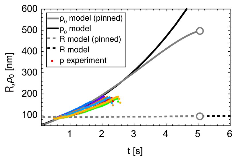
Figure 7: Comparison of measured (points) and predicted average bubble size $\rho_{0}$ as a function of time for several bubbles emerging from the same nucleation site (colors indicate different bubbles nucleating from the same site). Model results for unpinned (black) and pinned (gray) are shown along with the evolution of the radius of curvature $R$ (dashed). The open circle denotes the end of the validity of the pinned model.

Before comparing to experiment, we examine the impact of some of the key parameters in the model: the slope of the channel $\Phi$ and contact line viscosity $\xi$ in FIG. 5. We fix initial channel height $h_{0}=100$nm and supersaturation $\alpha=-4$. FIG. 5 depicts (A) the bubble size $\rho_{0}$, (B) the velocity of the bubble’s center of mass $\dot{X}$, (C) the radius of curvature R, and (D) the ratio of curvatures $R/\left(\rho_{0}+R\left(1-\sin\theta_{0}\right)\right)$ as functions of time when $\xi=10^{2}$ (gray line) and $10^{4}$ (black line) and when $\Phi=10^{-3.5}$ (solid line) and $10^{-4}$ (dashed line). The effect of the contact line viscosity is intuitive. The greater the dissipation at the contact line, the more the contact angle must be pushed out of equilibrium to achieve the same velocity leading to slower growth. Interestingly, changing the slope of the taper also changes the time at which the bubble will appreciably depart from its initial size. To understand why this is the case we consider the short time dynamics more closely.

Initially, the bubble grows slowly because it takes time for the contact line to move. Contact-line motion is needed to enable the Laplace pressure and the equilibrium concentration of the dissolved gas next to the bubble’s surface to decrease. At short times, before the contact line moves, the only way to accommodate mass is by decreasing $R$, which bulges the bubble further beyond the contact line, increasing Laplace pressure, slowing mass transfer. Thus at short times, contact line resistance introduces a negative feedback mechanism on bubble growth. This dynamic is apparent when examining the contact angle distribution at short times ($t<0.3$ s) in FIG. 6, the local contact angle $\theta\left(\psi,t\right)$ is for all $\psi$ less than the equilibrium contact angle $\theta_{0}$ indicating that the bubble has displaced fluid in all directions.

According to BH theory, such a contact angle distribution will causes the contact line to advance into the liquid (de-wet) and give way to the growing bubble. While this occurs at all points on the contact line initially, the contact angle distribution eventually breaks symmetry giving rising to a faster velocity at the leading edge, FIG. 6. As the interface at the leading edge moves $h$ increases, allowing $R$ to increase, the equilibrium concentration of the dissolved gas to decrease, and the mass transport to increase. In other words, the increasing channel height provides a positive feedback mechanism that accelerates the bubble’s growth once the contact line begins moving. The larger the opening slope or smaller the contact line viscosity, the quicker the switch between negative and positive feedback occurs. As the bubble’s geometry evolves, the contact angle distribution switches from being non-uniformly below the equilibrium contact angle $\theta_{0}$ (corresponding to de-wetting) to a portion of the rear contact line being greater than the equilibrium value. In other words, once the bubble begins translating down the conduit, de-wetting occurs at the leading edge ($\psi=0$), and wetting occurs at the trailing edge ($\psi=\pi$), FIG. 6 tracks the evolution of the contact angle at these two locations. The moment of the sign change of the trailing contact line is made clear in the inset of FIG. 6Bi (dashed lined).

Interestingly, while the velocity $\dot{X}$ initially increases (FIG. 5B), it achieves a maximum velocity and then slowly declines as $t\rightarrow\infty$. This velocity scaling is correlated with the aspect ratio $\varepsilon=R/\left(\rho_{0}+R\left(1-\sin\theta_{0}\right)\right)$ tending towards unity, indicating that the bubble’s geometry is becoming more spherical over time. Since this must also means that the contact angle distribution is becoming more uniform (tending towards $\theta\left(\psi\right)\rightarrow\theta_{0}$), we consider the limit of fast contact line relaxation $\eta_{\text{CL}}=0$ in the supplement. In this case, the contact angle is always uniform and at equilibrium; the bubble is therefore a spherical section that grows self-similarly and translates down the conduit at a velocity required to satisfy geometric constraints. In the supplement we show that $\dot{X}\propto t^{-1/2}$, just like FIG. 5B for large times. For the parameters used, our theory therefore predicts that confinement and contact line dynamics become less important once bubbles are on the order of $\sim$ 100 $\mu$m - 1 mm in extent.

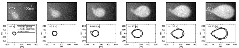
Figure 8: : (Top) Experimental observations of a bubble growing from a nucleation site (dashed white lines). (Bottom) Pinned (black lines, eqn. 11) and unpinned (dashed lines, eqn. 10) model predictions compared to contact line from top row (thick gray lines).

V Comparison with Experimental Observations

FIG. 7 compares our model predictions, with (gray) and without (black) pinning (modeled with the weighted eqn. 11 that smoothly interpolate between a completely pinned contact line at $\psi=\pi$ and full mobility at $\psi=0$), to experimental observations of bubbles that are pinned to their nucleation site (symbols). While we know the bubbles to be pinned, for comparison we show predictions made by both pinned and unpinned versions of the model. For both models, $\Phi=10^{-3}$, $h_{0}=80$nm, $\alpha=-2.9$, and $\xi=5.4$. FIG. 7A depicts $\rho_{0}$ (solid line) and $R$ (dashed line) as functions of time. When $t<10$s, we find no significant difference in the leading order growth rates predicted in the absence and presence of pinning. This is because the feedback of higher order geometric terms $\rho_{1,2,\cdots}$ on $R$ is weak when the bubble nearly circular. The open circle in FIG. 7 indicates the end of theoretical predictions for the pinned case; while the model fails at finite time, we note that in the experiment the bubble breaks apart prior to this point. In this paper, we do not consider instabilities that may lead to detachment. Before breakup, there is good qualitative agreement between the model and theory. In FIG. 8, we more closely compare the predicted geometry of the contact line to observations of the same data set. We see that the theoretical predictions are in good agreement with the observations away from the pinning/nucleation site (dashed circle).

Finally, in FIG. 9 we examine the relationship between the size $\rho_{0}$ and the projected aspect ratio $\mathscr{E}$ of the bubble (not to be confused the aspect ratio $\varepsilon$ plotted in FIG. 7D)

$$\mathscr{E}=\left(\rho_{0}-\rho_{2}+\rho_{4}\right)/\left(\rho_{0}+\rho_{2}+\rho_{4}\right)$$ (28)

where $\rho_{2,4}$ are shape corrections to $\rho_{0}$ (for $N=$5). We find that the faster growing bubbles (those with higher superstation) become elongated at smaller size. Our model therefore predicts that contact line dynamics and the tapered channel together introduce a growth rate-dependent geometric evolution, which would otherwise be absent in the zero capillary and Bond number regime we consider. Since bubble breakup likely depends on the extent to which the bubbles elongate, we posit that bubble creation frequency and departure size will depend on super-saturation. Our current single-curvature model does not allow us model the breakup mechanism. Before breakup, a neck forms which invalidates assumptions of our model; however, controlled experiments on droplet breakup in tapered conduits in the quasi-static regime strongly implicate a geometric instabilityDangla2013 .

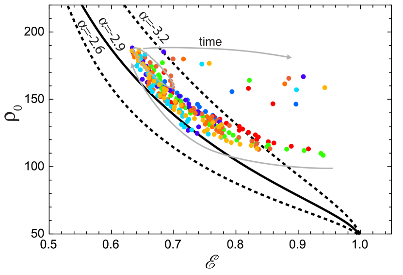
Figure 9: Model predictions (lines) of bubble size $\rho_{0}$ as a function of aspect ratio $\mathscr{E}$ (eqn. 28) for three different supersaturation values compared to experiment (points, colors indicate different bubbles nucleating from the same site). Arrows show the progression of time and circle highlights the point at which the bubbles break away from their nucleation sites ($t\sim$1-2 s).

VI Conclusion

We imaged and analyzed the growth and motion of sub-micron bubbles in a supersaturated liquid confined between two narrowly separated, rigid, diverging plates in the asymptotic limit of zero Capillary and Bond numbers. To enable imaging sub-micrometer-size bubbles, we used the experimental technique liquid cell electron microscopy to provide spatial and temporal resolution that is not readily available by any other types of microscopy. The motion of macroscopic bubbles is often driven by capillary and buoyancy forces, both of which are negligible at the length scales considered here. We hypothesize that bubble motion and growth are rate-limited by contact line dynamics. To predict contact line motion, bubble growth, and interface geometry, we use the Blake-Haynes mechanism to describe contact line motion as a function of contact angle. Variations in contact angle result from gas mass flow into the bubble under supersaturated conditions. Our theoretical predictions agree qualitatively with experimental observations. At early stages, bubbles grow slowly as contact line-mediated curvature mitigates the positive feedback mechanism that would otherwise enhance mass transfer into the bubble and drive rapid growth. This is somewhat similar to one of the more recent mechanisms that has been proposed to explain the longevity of surface-bound nano-bubbles; the pinning of the contact line controls curvature Weijs2013 ; Lohse2015a . At longer times, our model predicts that the growth rate of our bubbles accelerates due to positive feedback: decreased radius of curvature reduces the equilibrium gas concentration next to the bubbles’ surfaces, enhancing mass transport, and decreased confinement.

Our observations and model predictions have implications for various processes where bubbles nucleate and grow within surface defects, fissures, or tailored nanostructures such as are used for boiling and hydrolysis. Clearly, one could exploit geometry to clear bubbles; this much has been explored for microgravity applications Jenson2014 , albeit relying on driving forces that are negligible at the nanoscale as in our experiments.

Perhaps more intriguing is our model’s implication that bubble geometry depends on growth rate. This is somewhat unexpected given the overdamped regime but arises as the result of an additional time scale in the problem, the contact line relaxation. Growth-rate dependence is particularly apparent when aft contact line pinning is included in the model. Our prediction that the aspect ratio of growing teardrop bubbles can be controlled by controlling the supersaturation level is a novel mechanism that could be exploited in device design.

This paper has examined a fluid mechanical problem with the emerging experimental method of liquid cell electron microscopy. We demonstrate that liquid cell electron microscopy with its few nanometer and video-rate resolution can provide meaningful data that would be difficult, if not impossible, to obtain by other means. Although our liquid cell imaging provided qualitative information to support our theoretical predictions, the method is still at its infancy in terms of yielding quantitative data. Some calibration tools exist, for example the use of electron energy loss spectroscopy to measure liquid thickness Jungjohann2012 , but the accuracy is not sufficient for these types of experiments. We hope that in the future, liquid cells will be better equipped with diagnostic tools such as means to measure sufficiently accurately the distance between the confining plates and the conditions (pressure, temperature, chemical composition) of the liquid inside the liquid cell. Such developments would allow for better controlled experiments and will enable quantitative comparisons between theoretical predictions and experimental data.

VII Acknowledgements

The research was supported, in part, by the National Science Foundation CBET 1066573 and the Nano/Bio Interface Center through the National Science Foundation NSEC DMR08-32802. All movies were recorded by Joseph. M. Grogan at the IBM T. J. Watson Research Center.

References

- (1) P. G. Saffman and G. Taylor, “The Penetration of a Fluid into a Porous Medium or Hele-Shaw Cell Containing a More Viscous Liquid,” Proceedings of the Royal Society of London Series A, Mathematical and Physical Sciences, vol. 245, pp. 312–329, jun 1958.
- (2) G. Taylor and P. G. Saffman, “A note on the motion of bubbles in a hele-shaw cell and porour medium,” The Quarterly Journal of Mechanics and Applied Mathematics, vol. 12, pp. 265–279, jan 1959.
- (3) S. Tanveer and P. G. Saffman, “Stability of bubbles in a Hele–Shaw cell,” Physics of Fluids, vol. 30, pp. 2624–2635, sep 1987.
- (4) F. P. Bretherton, “The motion of long bubbles in tubes,” Journal of Fluid Mechanics, vol. 10, p. 166, mar 1961.
- (5) C. W. Park and G. M. Homsy, “Two-phase displacement in Hele Shaw cells: theory,” Journal of Fluid Mechanics, vol. 139, pp. 291–308, feb 1984.
- (6) S. J. Weinstein, E. B. Dussan, and L. H. Ungar, “A Theoretical-Study of 2-Phase Flow through a Narrow Gap with a Moving Contact Line - Viscous Fingering in a Hele-Shaw Cell,” Journal of Fluid Mechanics, vol. 221, no. 1990, pp. 53–76, 1990.
- (7) R. W. Style and E. R. Dufresne, “Static wetting on deformable substrates, from liquids to soft solids,” Soft Matter, jan 2012.
- (8) R. W. Style, Y. Che, S. J. Park, B. M. Weon, J. H. Je, C. Hyland, G. K. German, M. P. Power, L. a. Wilen, J. S. Wettlaufer, and E. R. Dufresne, “Patterning droplets with durotaxis,” Proceedings of the National Academy of Sciences of the United States of America, vol. 110, pp. 1–4, jun 2013.
- (9) M. K. Chaudhury and G. M. Whitesides, “How to Make Water Run Uphill,” Science, vol. 256, pp. 1539–1541, jun 1992.
- (10) H. A. Stone, “Engineering Flows in Small Devices: Microfluidics Toward a Lab-on-a-Chip,” Annual Review of Fluid Mechanics, vol. 37, pp. 425–455, jan 2005.
- (11) P. Renvoisé, J. W. M. Bush, M. Prakash, and D. Quéré, “Drop propulsion in tapered tubes,” EPL (Europhysics Letters), vol. 86, p. 64003, jun 2009.
- (12) R. Hanumanthu and K. J. Stebe, “Equilibrium shapes and locations of axisymmetric, liquid drops on conical, solid surfaces,” Colloids and Surfaces A: Physicochemical and Engineering Aspects, vol. 282-283, pp. 227–239, 2006.
- (13) L. Lorenceau and D. Qur, “Drops on a conical wire,” Journal of Fluid Mechanics, vol. 510, pp. 29–45, 2004.
- (14) R. M. Jenson, A. P. Wollman, M. M. Weislogel, L. Sharp, R. Green, P. J. Canfield, J. Klatte, and M. E. Dreyer, “Passive phase separation of microgravity bubbly flows using conduit geometry,” International Journal of Multiphase Flow, vol. 65, pp. 68–81, oct 2014.
- (15) T. Metz, N. Paust, R. Zengerle, and P. Koltay, “Capillary driven movement of gas bubbles in tapered structures,” Microfluidics and Nanofluidics, vol. 9, pp. 341–355, dec 2009.
- (16) E. Reyssat, “Drops and bubbles in wedges,” Journal of Fluid Mechanics, vol. 748, pp. 641–662, may 2014.
- (17) D. W. Langbein, Shape - Stability - Dynamics, in Particular Under Weightlessness. Springer Science & Business Media, jan 2002.
- (18) M. Alheshibri, J. Qian, M. Jehannin, and V. S. Craig, “A History of Nanobubbles,” Langmuir, vol. 32, pp. 11086–11100, nov 2016.
- (19) P. Ball, “Nanobubbles are not a superficial matter,” ChemPhysChem, vol. 13, pp. 2173–2177, may 2012.
- (20) V. S. J. Craig, “Very small bubbles at surfaces—the nanobubble puzzle,” Soft Matter, vol. 7, no. 1, pp. 40–48, 2011.
- (21) C.-K. Fang, H.-C. Ko, C.-W. Yang, Y.-H. Lu, and I.-S. Hwang, “Nucleation processes of nanobubbles at a solid/water interface,” Scientific Reports, vol. 6, p. 24651, apr 2016.
- (22) G. Liu, Z. Wu, and V. S. J. Craig, “Cleaning of Protein-Coated Surfaces Using Nanobubbles: An Investigation Using a Quartz Crystal Microbalance,” The Journal of Physical Chemistry C, vol. 112, pp. 16748–16753, oct 2008.
- (23) G. Liu and V. S. J. Craig, “Improved Cleaning of Hydrophilic Protein-Coated Surfaces using the Combination of Nanobubbles and SDS,” ACS Applied Materials & Interfaces, vol. 1, pp. 481–487, feb 2009.
- (24) S. Yang and A. Duisterwinkel, “Removal of Nanoparticles from Plain and Patterned Surfaces Using Nanobubbles Removal of Nanoparticles from Plain and Patterned Surfaces Using Nanobubbles,” Applied Scientific Research, vol. 27, pp. 11430–11435, sep 2011.
- (25) L. Dong, X. Quan, and P. Cheng, “An experimental investigation of enhanced pool boiling heat transfer from surfaces with micro/nano-structures,” International Journal of Heat and Mass Transfer, vol. 71, pp. 189–196, apr 2014.
- (26) A. Fazeli, M. Mortazavi, and S. Moghaddam, “Hierarchical biphilic micro / nanostructures for a new generation phase-change heat sink,” Applied Thermal Engineering, vol. 78, pp. 380–386, 2015.
- (27) E. N. W. Kuan-Han Chu, Ryan Enright, “Structured surfaces for enhanced pool boiling heat transfer,” Applied Physics Letters, vol. 100, no. 24, p. 241603, 2012.
- (28) W. B. Cai, H. L. Yang, J. Zhang, J. K. Yin, Y. L. Yang, L. J. Yuan, L. Zhang, and Y. Y. Duan, “The Optimized Fabrication of Nanobubbles as Ultrasound Contrast Agents for Tumor Imaging,” Scientific Reports, vol. 5, no. 1, p. 13725, 2015.
- (29) M. P. P.S. Epstein, P. S. Epstein, and M. S. Plesset, “On the Stability of Gas Bubbles in Liquid-Gas Solutions,” The Journal of Chemical Physics, vol. 18, p. 1505, jan 1950.
- (30) S. Ljunggren and J. C. Eriksson, “The lifetime of a colloid-sized gas bubble in water and the cause of the hydrophobic attraction,” Colloids and Surfaces A: Physicochemical and Engineering Aspects, vol. 129-130, pp. 151–155, feb 1997.
- (31) X. H. Zhang, A. Quinn, and W. A. Ducker, “Nanobubbles at the Interface between Water and a Hydrophobic Solid,” Langmuir, vol. 24, pp. 4756–4764, may 2008.
- (32) J. R. T. Seddon and D. Lohse, “Nanobubbles and micropancakes: gaseous domains on immersed substrates,” Journal of Physics: Condensed Matter, vol. 23, p. 133001, apr 2011.
- (33) Y. Sun, G. Xie, Y. Peng, W. Xia, and J. Sha, “Stability theories of nanobubbles at solid-liquid interface: A review,” Colloids and Surfaces A: Physicochemical and Engineering Aspects, vol. 495, pp. 176–186, apr 2016.
- (34) N. D. Petsev, M. S. Shell, and L. G. Leal, “Dynamic equilibrium explanation for nanobubbles’ unusual temperature and saturation dependence,” Physical Review E - Statistical, Nonlinear, and Soft Matter Physics, vol. 88, pp. 10402–10405, jul 2013.
- (35) A.-J. Choi, C.-J. Kim, Y.-J. Cho, J.-K. Hwang, and C.-T. Kim, “Effects of surfactants on the formation and the stability of Capsaicin-loaded nanoemulsion,” Langmuir, vol. 28, pp. 10471–10477, jul 2012.
- (36) J. H. Weijs and D. Lohse, “Why surface nanobubbles live for hours,” Physical Review Letters, vol. 110, pp. 54501–54505, jan 2013.
- (37) D. Lohse and X. Zhang, “Surface nanobubbles and nanodroplets,” Reviews of Modern Physics, vol. 87, no. 3, pp. 981–1035, 2015.
- (38) S. Maheshwari, M. van der Hoef, X. Zhang, and D. Lohse, “Stability of Surface Nanobubbles: A Molecular Dynamics Study.,” Langmuir : the ACS journal of surfaces and colloids, p. acs.langmuir.6b00963, apr 2016.
- (39) J. M. Grogan, N. M. N. Schneider, F. M. Ross, and H. H. Bau, “Bubble and pattern formation in liquid induced by an electron beam.,” Nano Letters, vol. 14, pp. 359–64, jan 2014.
- (40) T. D. Blake and J. M. Haynes, “Kinetics of liquidliquid displacement,” Journal of Colloid and Interface Science, vol. 30, pp. 421–423, jan 1969.
- (41) T. D. Blake, “The physics of moving wetting lines,” Journal of colloid and interface science, vol. 299, pp. 1–19, jul 2006.
- (42) D. M. Kaz, R. McGorty, M. Mani, and M. P. Brenner, “Physical ageing of the contact line on colloidal particles at liquid interfaces,” Nature materials, jan 2012.
- (43) F. Brochard-Wyart and P. G. de Gennes, “Dynamics of partial wetting,” Advances in colloid and interface science, vol. 39, pp. 1–11, oct 1992.
- (44) J. M. Grogan and H. H. Bau, “The Nanoaquarium: A Platform for In Situ Transmission Electron Microscopy in Liquid Media,” Journal of Microelectromechanical Systems, vol. 19, pp. 885–894, aug 2010.
- (45) J. M. Grogan, L. Rotkina, and H. H. Bau, “In situ liquid-cell electron microscopy of colloid aggregation and growth dynamics,” Physical Review E - Statistical, Nonlinear, and Soft Matter Physics, vol. 83, p. 61405, jun 2011.
- (46) N. M. Schneider, M. M. Norton, B. J. Mendel, J. M. Grogan, F. M. Ross, and H. H. Bau, “Electron–Water Interactions and Implications for Liquid Cell Electron Microscopy,” The Journal of Physical Chemistry C, vol. 118, pp. 22373–22382, sep 2014.
- (47) F. M. Ross, “Opportunities and challenges in liquid cell electron microscopy,” Science, vol. 350, no. 6267, pp. 1–10, 2015.
- (48) D. Bhattacharya, M. Bosman, V. R. Mokkapati, F. Y. Leong, and U. Mirsaidov, “51.Nucleation Dynamics of Water Nanodroplets,” Microscopy and Microanalysis, vol. 20, pp. 407–415, mar 2014.
- (49) U. M. Mirsaidov, H. Zheng, D. Bhattacharya, Y. Casana, and P. Matsudaira, “Direct observation of stick-slip movements of water nanodroplets induced by an electron beam,” in Proceedings of the National Academy of Sciences, vol. 109, pp. 7187–7190, 2012.
- (50) U. M. Mirsaidov, C.-D. Ohl, and P. Matsudaira, “A direct observation of nanometer-size void dynamics in an ultra-thin water film,” Soft Matter, pp. 7108–7111, 2012.
- (51) E. R. White, M. Mecklenburg, S. B. Singer, and B. C. Regan, “Creation And Manipulation Of Bubbles In Liquid Water Using A Scanning Transmission Electron Microscope,” Microscopy and Microanalysis, vol. 18, pp. 1102–1103, nov 2012.
- (52) N. M. Schneider, J. H. Park, M. M. Norton, F. M. Ross, and H. H. Bau, “Automated analysis of evolving interfaces during in situ electron microscopy,” Advanced Structural and Chemical Imaging, vol. 2, p. 2, feb 2016.
- (53) D. Blair and E. Dufresne, “Matlab Particle Tracking.”
- (54) B. Arkles, “Hydrophobicity, Hydrophilicity and Silanes,” Paint and Coatings Industry, pp. 114–135, 2006.
- (55) R. Sander, “Compilation of Henry’s law constants (version 4.0) for water as solvent,” Atmospheric Chemistry and Physics, vol. 15, pp. 4399–4981, jan 2015.
- (56) E. L. Cussler, Diffusion: Mass Transfer in Fluid Systems. Cambridge, UK: Cambridge University Press, 3 ed., 2009.
- (57) P. G. Petrov, “Dynamics of deposition of Langmuir–Blodgett multilayers,” Journal of the Chemical Society, jan 1997.
- (58) J. C. Berg, The Bridge to Nanoscience. World Scientific, jan 2010.
- (59) R. Dangla, S. C. Kayi, and C. N. Baroud, “Droplet microfluidics driven by gradients of confinement,” Proceedings of the National Academy of Sciences, vol. 110, pp. 853–858, jan 2013.
- (60) D. Lohse and X. Zhang, “Pinning and gas oversaturation imply stable single surface nanobubbles,” Physical Review E, vol. 91, p. 31003, mar 2015.
- (61) K. L. Jungjohann, J. E. Evans, J. A. Aguiar, I. Arslan, and N. D. Browning, “Microscopy Microanalysis Atomic-Scale Imaging and Spectroscopy for In Situ Liquid Scanning Transmission Electron Microscopy,” pp. 621–627, 2012.