Parameterizing the Supernova Engine and its Effect on Remnants and Basic Yields

Abstract

Core-collapse supernova science is now entering an era where engine models are beginning to make both qualitative and quantitative predictions. Although the evidence in support of the convective engine for core-collapse supernova continues to grow, it is difficult to place quantitative constraints on this engine. Some studies have made specific predictions for the remnant distribution from the convective engine, but the results differ between different groups. Here we use a broad parameterization for the supernova engine to understand the differences between distinct studies. With this broader set of models, we place error bars on the remnant mass and basic yields from the uncertainties in the explosive engine. We find that, even with only 3 progenitors and a narrow range of explosion energies, we can produce a wide range of remnant masses and nucleosynthetic yields.

1. Introduction

A core-collapse supernova is produced when the core of a massive star collapses under its own weight, forming a neutron star. The gravitational potential energy released in this collapse is $2-3\times 10^{53}$ erg. Extracting 1% of this energy has been the focus of core-collapse engine astronomers for the past 80 years (Burrows, 2013). The current favored engine behind supernova invokes convection above the neutron star formed in the collapse. When the collapse of the core is stopped by nuclear forces and neutron degeneracy pressure, it sends a bounce shock through the star that quickly stalls. The region between the proto-neutron star and the stalled shock is convectively unstable (Herant et al., 1994). An increasing number of simulations have produced explosions under this paradigm, and it has slowly gained traction and become the leading theory model for the supernova engine (Fryer & Young, 2007; Takiwaki et al., 2014; Melson et al., 2015; Lentz et al., 2015; Burrows et al., 2016).

Additionally, the observational support for the convective supernova engine continues to grow (for a review, see Fryer et al. 2017, submitted). One of the strongest pieces of evidence demonstrating that at least some supernovae are powered by this convective engine is the recent observations of the ⁴⁴Ti distribution in the Cassiopeia A remnant (Grefenstette et al., 2014, 2017). Unlike other elements observed in supernova remnants that emit only when they are shock heated, the NuSTAR observations detect decay lines from ⁴⁴Ti, observing all of the ⁴⁴Ti, including unshocked material. Since ⁴⁴Ti is produced in the innermost ejecta, it provides an ideal probe of the engine asymmetries. The multi-mode but not bimodal structure of the ⁴⁴Ti distribution observed by NuSTAR not only requires engine asymmetries, but rules out the jet/magnetar engines for the supernova that produced the Cassiopeia A remnant (Grefenstette et al., 2014). With these observations, the convective engine is now the clear leading theory for supernova explosions.

Many details of this convective engine remain unknown. For example, the time it takes to drive an explosion varies with simulations. Similarly, the explosion energy is sensitive to the simulation details. The uncertainties lead to a range of predictions for the remnant masses and yields of a given progenitor. Accurate remnant masses and yield measurements may provide clues to the nature of this convective engine, but to understand these clues, we must first understand the range of results from this engine paradigm.

In this paper, we develop a broadly parameterized model to study more fully the possible solutions from the convection-enhanced supernova engine. To capture the convective engine more accurately, we implement a 3-part parameterization for the energy injection: power, duration and the extent of the energy injection region. With these models, we produce a range of explosion energies, compact remnant masses, and nucleosynthetic yields. In Section 2, we describe details of past remnant mass calculations including aspects of the explosion that set the mass of the compact remnant. Section 3 describes our progenitors and our method to implement explosions. In Section 4, we review the results of our simulation suite, studying both the remnant mass and key yields typically observed in supernova remnants. Without constraints, a wide range of results are possible. By limiting the allowed explosion energy, we place constraints on the remnant mass and yields, and we conclude by comparing these constrained results to current remnant mass and remnant yield observations.

2. Remnant Masses

The supernova explosion directly determines the fate of the compact remnant. In one extreme, if an explosion is unable to launch, material accretes onto the proto-neutron star, ultimately causing it to collapse to form a black hole. Without an explosion or further ejection, the entire star accretes onto the black hole, forming a black hole mass equal to the mass of the star at collapse. Instead, if a strong explosion is produced, the material above the proto-neutron star is ejected leaving behind a neutron star with a mass set to that of the proto-neutron star. In between these two extremes in the explosion energy, a range of remnant masses can be produced.

Initial remnant mass distributions were based solely on the structure of the progenitor star (Timmes et al., 1996) guided by nucleosynthetic yield requirements. Such estimates did not include an understanding of the explosion mechanism itself. More recent remnant-mass estimates have included constraints based on the supernova engine. For most of these, the method has focused on increasing the energy deposition due to neutrinos (Fröhlich et al., 2006; Fischer et al., 2010; Ugliano et al., 2012; Ertl et al., 2016; Sukhbold et al., 2016). For example, Perego et al. (2015) tap energy from the $\mu$ and $\tau$ neutrinos, calibrating their model by fitting SN 1987A. With these calibrated engines, they can produce a “best-set” of explosion models versus progenitor mass. These models typically still deposit the energy at the neutrino gain region. In the supernova engine, convection can redistribute the energy across the entire convective engine. Here we want to probe the broader range of explosion possibilities where we include this redistribution of the energy.

Initial models considering these effects were done analytically. The energy of the convective engine model can be estimated by determining the energy stored in the convection region when pressure of this region overcomes the pressure of the infalling star. The corresponding explosion energies from this analysis are a few times 10⁵¹ erg, explaining why most supernova energies also lie in this range (even though 10⁵³ erg of gravitational potential energy is released in the collapse). With estimates based on this convective engine, Fryer & Kalogera (2001) and Fryer et al. (2012) predicted the remnant mass as a function of progenitor mass for a range of different stellar evolution models. Another approach has been to induce explosions in 1-dimensional models and calculate the yields and remnant masses from these explosions. The problem with this latter technique is that the results vary wildly upon how the explosion is induced. In this work, we strive to better understand how much the results can vary within the convective paradigm and our parameterized models are designed to produce a full range of results. From this range, we can use observational constraints to limit our explosion models.

The processes that set the remnant mass can be separated into 3 basic phases: the core mass post-bounce, the timing of the explosion and the fallback post-explosion. As electron capture produces a runaway collapse, the core collapses. When the core approaches nuclear densities, strong nuclear forces and neutron degeneracy pressure halt the infall, producing a bounce. When the bounce shock moves outward, it leaves behind a dense core, the seed of the proto-neutron star. The bounce of the core depends upon the entropy and for rapidly-spinning stars, the rotation in the core. The masses of this initial proto-neutron star are typically $\sim 0.9\pm 0.2\,M_{\odot}$(Fryer et al., 2012).

After the stall of the bounce shock, the region between the dense core and the stalled shock is typically unstable to Rayleigh-Taylor instabilities. Other instabilities can also exist, most notably the standing accretion shock instability (Houck & Chevalier, 1992; Blondin et al., 2003). During this phase, material from the collapsing star is transported down to the proto-neutron star and is assimilated onto this core. This phase continues until either the energy in this convective region is sufficient to drive an explosion or the proto-neutron star collapses to form a black hole. The longer it takes to explode, the larger the proto-neutron star core becomes. By modifying the onset of the energy deposition and its power, our simulations produce a range of remnant masses at the launch of the explosion. If the mass exceeds the maximum neutron star mass, the core will collapse to form a black hole with no explosion. The most massive stellar-mass black holes are formed in these failed explosions.

If the energy in the convective region is sufficent to drive an explosion, the infalling material is pushed outward. This explosion shock decelerates as it pushes outward, causing its velocity to drop below the escape velocity. This material will ultimately fall back onto the proto-neutron star (Colgate, 1971; Fryer, 2006). This fallback accretes onto the neutron star and is responsible for making high-mass neutron stars and low-mass black holes. We follow our explosions out to 4000 s at which time we can determine which material will fall back (based on the escape velocity) and accurately calculate the final remnant mass.

3. Simulations

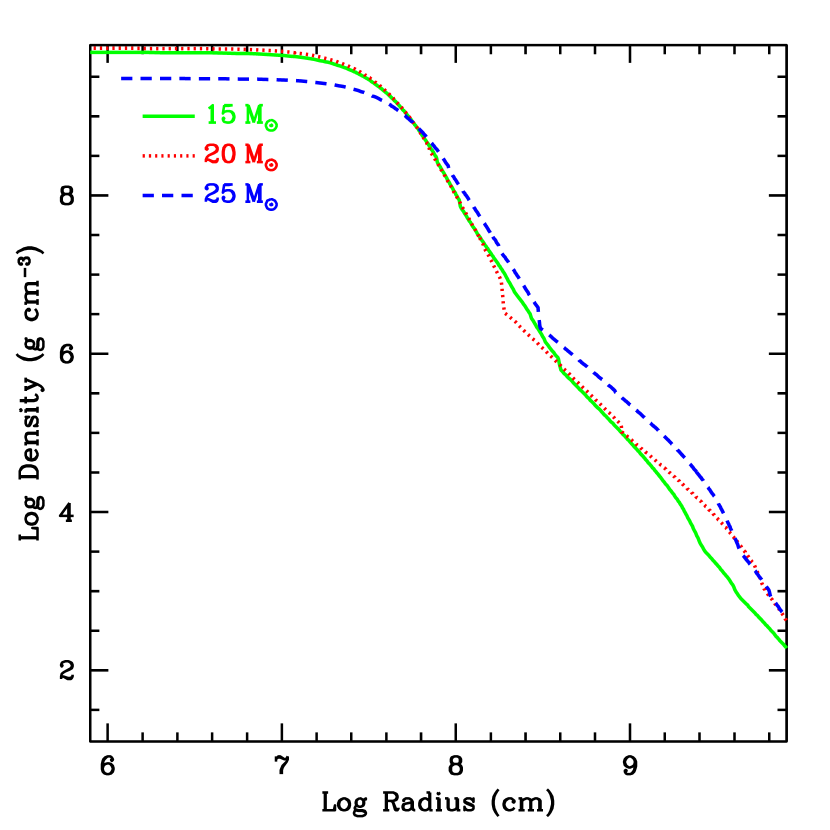
Figure 1.— Log density versus log radius for our 3 progenitor models: 15 M_⊙ (solid), 20 M_⊙ (dotted), 25 M_⊙ (dashed). The peak density is more a reflection of the extent of the collapse and less on the structure of the star. The slight changes in the slope between the different star shows the more compact structure of the 25 M_⊙ star. The decrease in the 20 M_⊙ density above $10^{8}$ cm reflects a jump in the entropy of the star at that point. In that sense, the 20 M_⊙ star might be easier to explode than the 15 M_⊙ star.

In this paper, we focus on the fate of stellar collapse as a function of the energy injection in the supernova engine. By studying a wide range of injection engines, we can study trends in the remnant mass and final supernova yields as a function of explosion energy. For this study, we use 3 different progenitor masses (15, 20, and 25 $M_{\odot}$) computed using the KEPLER code (Weaver et al., 1978; Woosley et al., 2002; Heger & Woosley, 2010). We chose these as representative models for exploding systems where the convective engine can produce a range of results. For low-mass core-collapse systems (roughly 8-10 M_⊙), the envelope is so weakly bound (Ibeling & Heger, 2013; Woosley & Heger, 2015) that an explosion typically occurs quickly with little fallback (Kitaura et al., 2006). It is unlikely that there is a lot of variation in the engine for these progenitors. Likewise, for stars with minimal mass loss with masses above 30 M_⊙, most simulations predict that the convective engine fails to drive an explosion (Fryer, 1999; Heger et al., 2003; O’Connor & Ott, 2013; Sukhbold et al., 2016), although see Müller et al. (2016b)

For these calculations, a $19$-species nuclear network (Weaver et al., 1978) is used at low temperatures (until the end of oxygen burning); for silicon burning band beyond, KEPLER switches to a quasi-equilibrium approach that provides an efficient and accurate means to treat silicon burning including convection and then transitions to a nuclear statistical equilibrium network after silicon depletion. For convection we use the Ledoux criterion and mixing length theory. For semiconvection we use a diffusion coefficient which is 10% that of thermal diffusion, which roughly corresponds to the to the efficiency resulting from the formulation by Langer et al. (1983) with an $\alpha$ value of $0.04$. We also include thermohaline mixing according (Heger et al., 2005), but the process has no major impact on the models. All processes are formulated for use with a general equation of state (see Appedix in Heger et al. 2005) and mixing is implemented as a diffusive processes. For consistency with prior work the initial composition is taken from Grevesse & Noels (1993). The models are the same as presented in Jones et al. (2015) but evolved to the presupernova stage.

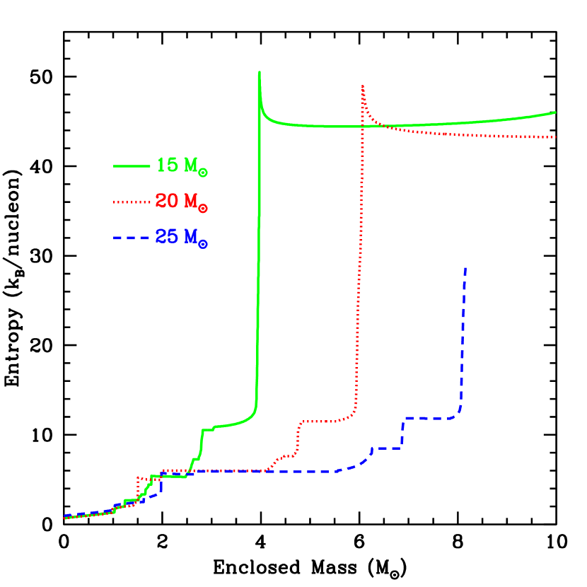
Figure 2.— Entropy versus enclosed mass for our 3 progenitors: 15 M_⊙ (solid), 20 M_⊙ (dotted), 25 M_⊙ (dashed). The jumps in entropy typically mark convective zone, and hence, composition boundaries.

Figure 1 shows the density profiles of our 3 progenitor stars. Although the inner density mostly shows the extent of the collapse (the core of the 25 M_⊙ has not collapsed as deeply into its potential well), the outer densities show the more compact structure of the 25 M_⊙ star. The sharp decrease in the density of the 20 M_⊙ above $10^{8}$ cm reflects the entropy jump in the star at this radius. This is easier to see in the entropy profiles shown in Figure 2. At roughly 1.5 M_⊙, the entropy in the 20 M_⊙ rises sharply. This corresponds to the lower-edge of the oxygen-burning shell which may produce the seeds to convection within the supernova engine (Müller et al., 2016b).

Our simulations are set up to mimic the basic convective-engine paradigm with our 1-dimensional models. In fast rotating models, centrifugal support can slow the collapse before the material reaches nuclear densities, causing it to bounce at a lower density Mönchmeyer & Müller (1989); Fryer & Heger (2000) and our 1-dimensional models would not capture the collapse/bounce phase. At still higher rotation speeds, disks can form around the collapsed core. In both cases, the angular momentum profiles from these collapses produce sub millisecond pulsars and it is likely that such explosions are rare. Unless the core is rapidly rotating, the collapse and bounce phase can be modeled reasonably accurately in 1-dimension. Our 1-dimensional collapse code utilizes a Lagrangian hydrodynamics scheme coupled to gray neutrino transport with 3 neutrino species: electron, anti-electron, $\mu+\tau$ neutrinos (Herant et al., 1994; Fryer et al., 1999). This code includes general relativistic effects (spherically symmetric), an equation of state for dense nuclear matter combining the Swesty-Lattimer equation of state at high densities (Lattimer & Douglas Swesty, 1991) and the Blinnikov equation of state at low densities (Blinnikov et al., 1996), and an 18-isotope nuclear network (Fryer et al., 1999). With this code, we follow the collapse and bounce of the core of our core-collapse progenitors.

Within the convection-enhanced neutrino-driven supernova paradigm, energy from the hot proto-neutron star and the continually accreting material drives convection. If the convection is rapid, this energy is redistributed across the entire convective region. To mimic this explosion process, we have introduced a series of parameters including the region into which the energy is deposited (representing the size of the convective region) as well as the energy deposition rate. In the simplest models, once the explosion is launched, energy deposition halts. Material can continue to accrete even after the launch of the shock. This fallback material can drive further outflows, depositing additional energy (Fryer, 2009) and are seen in many multi-dimensional core-collapse calculations (e.g., Lentz et al., 2015). To include this effect, we allow a broad range of durations, including calculations that allow a time-dependent energy-deposition rate. Although this allows us to include more properties of the convective engine than past studies, bear in mind that these are still 1-dimensional simulations and do not include the full effects of multi-dimensional calculations.

Finally, we have included a small number of models for our most-massive progenitor that have extremely late-time energy depositions. Late-time energy deposition can either be through late-time fallback or some magnetically-driven engine, e.g. magnetar.

We vary many of the parameters independently. But, in an actual engine, some parameters depend upon each other. For example, a higher-power drive will produce more vigorous convection and can produce a larger convective region. Similarly, a weak drive likely ultimately produces a smaller convective region. But other factors (like the initial seeds and rotation) can also affect the size of the convective region. Hence, for this paper, we vary these parameters independently. Likewise, a strong explosion is likely to have a shorter deposition time. Our parameter space allows a strong explosion with a long deposition time. In this manner, we produce stronger explosions than one would expect with the convective engine. In such cases, our models do not represent the classic convective engine alone, rather mimicking magentically-driven or fallback energy sources. If we limited the results to the classic convective engine, we could constrain our parameters somewhat.

4. Results

4.1. Compact Remnant Masses

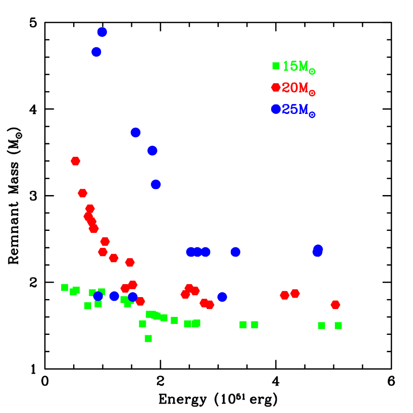
Figure 3.— Remnant mass versus explosion energy for our 3 progenitor masses: 15 M_⊙ (square), 20 M_⊙ (hexagon), 25 M_⊙ (circle).

Ideally, for a given progenitor star, there would be a one-to-one correspondence between explosion energy and remnant mass. The convective engine depends upon the growth of the convective instabilities that, in turn, depend upon a variety of features of the progenitor, including the progenitor’s rotation and the magnitude of the turbulence in the progenitor’s burning layers. The asphericities in the burning layers provide the seeds for the convection in the engine. These seemingly small differences can cause large differences in the growth of the convective motions above the proto-neutron star, leading to a wide range of explosion energy for roughly similar progenitors: see, for example, Couch & Ott (2015). Therefore, it is possible that progenitors of equal mass can produce very different explosion energies.

The explosion energy is set to the kinetic energy minus the absolute value of the gravitational potential energy 4000 s into the explosion. But because the nature of the explosion can vary wildly, this may not be the case. Table 1 shows the different choices for the energy deposition and the resultant compact masses. There are multiple injection parameters that produce roughly the same explosion energy. In this manner, we can determine whether the yields only depend upon the explosion energy and progenitor, or whether the nature of the explosion can alter the yield.

Figure 3 plots remnant mass versus explosion energy for these models. These masses are given in bayronic mass of the collapsing core. The gravitational mass of the remnant is likely to be $\sim$10-15% lower. Hence, our 15 M_⊙ progenitor produces remnants with gravitational masses in the 1.2-1.7 M_⊙ range. More massive progenitors generally produce more massive remnants (Fryer, 1999): for explosions between $1-2\times 10^{51}$ erg, remnant masses can be as high as 2 M_⊙ for a 20 M_⊙ progenitor and over 4 M_⊙ for a 25 M_⊙ progenitor

Because fallback is less in stronger explosions (Fryer et al., 2012), there is a clear trend where more energetic explosions produce lower mass remnants. Similarly, the high binding energy of more massive stars means that, for a fixed explosion energy, the more massive progenitors generally produce more massive remnants. Indeed, with our normal explosion methods, the remnant mass for our 25 M_⊙ progenitor with “standard” supernova explosion energies of $1-2\times 10^{51}$ erg produce remnants with gravitational masses ranging from 2 to 4.25 M_⊙. For a few times $10^{50}$ erg explosion, most of the 25 M_⊙ star remains bound, making a large black hole.

Table 1 shows the wide range of total injection energies in our models. As energy is injected into the layers above the proto-neutron star, this region begins to emit neutrinos copiously. Hence, the injection energy can be much higher than the final explosion energy. Explosion energies above a few times $10^{51}$ erg are difficult to achieve without extremely high injection energies and it is unlikely that these high energies occur without a different engine.

Recent results from Sukhbold et al. (2016) argue that they can make $<2$ M_⊙ remnants with progenitor systems with initial masses above 20 M_⊙ with $10^{51}$ erg explosions. These explosions are driven by enhanced neutrino energy deposition. The neutrino deposition region is typically very close to the surface of the proto-neutron star and these models closely mimic our small injection-region models. However, our standard explosions, with energy injections less than 1 s were unable to reproduce these results. Either these progenitors are very different than ours (have much less compact cores) or our models are missing some aspect of the explosion. One solution is that late-time energy injection prevents the fallback. We were able to reproduce more modest remnant masses by constructing explosions with long-term energy injection. In a scenario where continued accretion through fallback or magnetar dipole radiation inject energy at late times, we can minimize the fallback and the final remnant mass. In such a scenario, we can produce gravitational masses below 1.6 M_⊙ even for $<10^{51}$ erg explosions.

Our progenitors are all modeled as single stars. Wind mass loss ejects half of the mass in our 25 M_⊙ star, 7 M_⊙ of our 20 M_⊙ star and 4.5 M_⊙ in our 15 M_⊙ star. Binary mass transfer can remove the hydrogen and even helium envelopes allowing further mass loss through winds. If this mass loss affects the core, it will alter the fate of the collapse. If it does not alter the inner $\sim$3 M_⊙, the explosion is not affected by the mass loss and, unless there is considerable fallback, neither is the remnant mass. If mass loss does alter the core structure (e.g. it occurs before helium depletion in the core) or fallback is extensive, binary mass transfer can dictate the final remnant mass.

Our predictions include a few additional uncertainties. We choose when to start driving the energy after the bounce - the timing is determined by the instability growth time. This reflects the time for the convection to develop between the proto-neutron star and the stalled shock. Altering this can change the final remnant mass by 0.1-0.2 M_⊙. In addition, after the launch of the shock, we “accrete” onto the proto-neutron star after the material exceeds a density of between 10${}^{10}-10^{12}$ g cm^-3, arguing that above this density, neutrino cooling is rapid, allowing it to accrete quickly. For models with over a solar mass of fallback and late-time drives, this density limit can also change the mass by 0.1-0.2 M_⊙ (the mass increases with a larger density limit).

4.2. Basic Yields

The yields from a given progenitor are also sensitive to the details of the explosion. For this paper, we use the publicly available TORCH code (Timmes et al., 2000) (http://cococubed.asu.edu) to post-process our ejecta trajectories and calculate a few basic yields from the supernova explosion: oxygen, neon, magnesium, silicon, sulfur, argon, calcium, and iron peak elements using a 489 isotope network. The initial abundances are taken from the network in our stellar models, limited to 19 isotopes (mostly alpha-chain, including the 8 isotopes considered here). For these nuclear network calculations, we use the first 2000 (equally-spaced, 10 ms) timesteps, following the ejecta for 20 s, well after nuclear burning is complete. The Torch code sub-samples these time dumps if more resolution is needed. Both the choice of the initial abundances and this time sampling will be discussed in more detail in a later paper (Andrews et al., in preparation). These calculations are intended to demonstrate the range in yields. The exact yields will vary with a more complete isotope distribution in the initial conditions and understanding the nucleosynthetic yield errors must also include errors in the initial composition, time sampling, network conditions (see Andrews et al., in preparation).

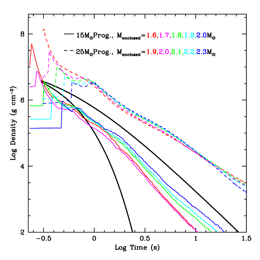
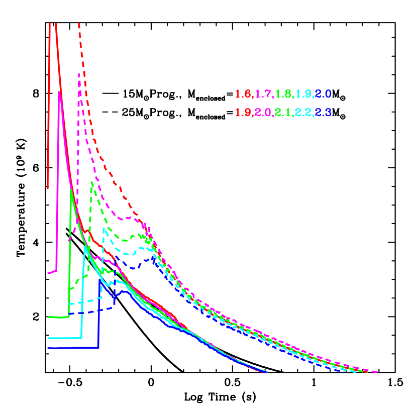
Figure 4.— Density and temperature versus time for ejected matter. These trajectories are taken for matter at a range of positions (denoted by the enclosed mass) within the star with mass coordinates ranging from the base of the ejected material through the oxygen layer (the innermost layers have the highest peak densities and temperatures). Note that additional shocks can both increase the density and temperature with time and the trajectories are not necessarily monotonic. On top of these curves are the standard analytic fits to the trajectory evolution.

As the supernova explosion plows through the star, the shock hitting the stellar material accelerates it while compressing and heating it. The shock-heated material then adiabatically cools as the star expands. The final yields are set by the peak temperature and density at this peak temperature as well as the timescale of the cooling. Typically, astronomers use one of two profiles, both assuming adiabatic expansion, but with different expansion evolutions(Magkotsios et al., 2010; Harris et al., 2017). Originally, an exponential decay was assumed(Hoyle et al., 1964; Fowler & Hoyle, 1964):

$$T=T_{0}e^{-t/\tau}$$ (1)

and

$$\rho=\rho_{0}e^{-t/3\tau}$$ (2)

where the pre-shock temperature and density are $T_{0}$ and $\rho_{0}$ and a decay time $\tau=(446/\rho_{0}^{0.5})$. Comparisons to explosion calculations suggests an alternative, constant-velocity expansion that produces a power-law evolution(Magkotsios et al., 2010) similar to some wind calculations(Panov & Janka, 2009):

$$T=T_{0}/(2t+1)$$ (3)

and

$$\rho=\rho_{0}/(2t+1)^{3}.$$ (4)

Figure 4 shows temperature and density profiles for a set of mass points for two different explosions (strong explosions of a 15 M_⊙ and 25 M_⊙ progenitor). Although the power law evolution is the better fit to the data, especially after the ejecta drops out of nuclear statistical equilibrium where the time evolution is most critical, neither analytic model captures all aspects of the expansion. In particular, a succession of shocks can actually cause the temperature and density to increase as the material expands and the evolution is not necessarily monotonic.

The yields for our models are listed in Table 2. The star itself produces many of the yields studied here during its lifetime. One of the affects of the supernova explosion is to determine what material is ejected and what remains part of the compact remnant. But the shocks in the supernovae can drive nuclear burning, further altering the abundances in the star, both destroying and producing the elements in this study. For example, when the supernova shock hits the silicon layer, it drives fusion, producing iron and destroying silicon. Silicon, on the other hand, can be produced when the shock heats the oxygen shell.

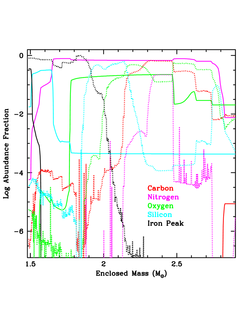
Figure 5.— Abundance fractions of carbon, nitrogen, oxygen, silicon and iron peak elements as a function of enclosed mass both at collapse (solid) and after the supernova explosion (dotted) for model M15bE5.08: a 15 M_⊙ progenitor with a 5 foe explosion (see Table 1 for characteristics). The strong shock in this explosion produces roughly 0.5M_⊙ of iron peak elements.

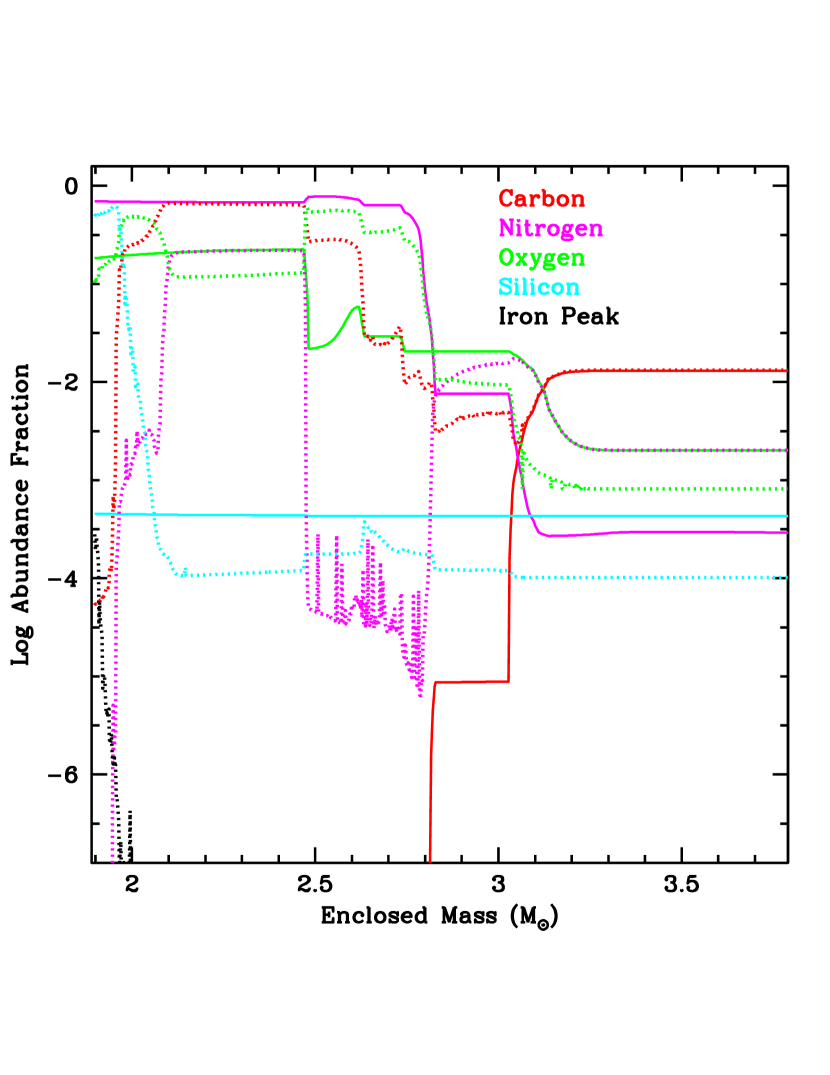
Figure 6.— Abundance fractions of carbon, nitrogen, oxygen, silicon and iron peak elements as a function of enclosed mass both at collapse (solid) and after the supernova explosion (dotted) for model M15aE0.54: a 15 M_⊙ progenitor with a 0.5 foe explosion (see Table 1 for characteristics). Even in this weak explosion where much of the inner region falls back on the compact remnant, the explosion resets the innermost ejecta.

Stellar yields, shock-driven nuclear burning in the supernova, and the amount of ejected material all play an important role in the nucleosynthetic yields of supernovaee. To compare the different roles these 3 factors have on the nucleosynthetic yields, we focus on two explosions of our 25 M_⊙ progenitor. Figure 5 shows the abundance fraction of carbon, nitrogen, oxygen, silicon and iron peak elements for model M15bE5.08 (a 15 M_⊙, $5\times 10^{51}$ erg explosion, see Table 1 for characteristics) at collapse and after the supernova shock has passed through it. Although the pre-collapse star sets the initial seeds for nuclear burning, this strong explosion alters the abundance fraction for the entire inner material in the star, producing roughly 0.5M_⊙ of iron peak elements. In the weak explosion (model M15aE0.54: a 15 M_⊙, $0.5\times 10^{51}$ erg explosion), much of the material synthesized in the shock falls back onto the newly-formed neutron star (Figure 6). The innermost ejecta are also determined by the supernova shock. In both cases, the outermost material is set by the pre-collapse progenitor.

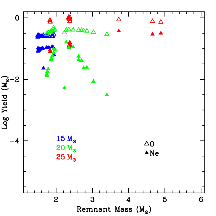
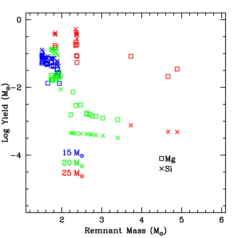
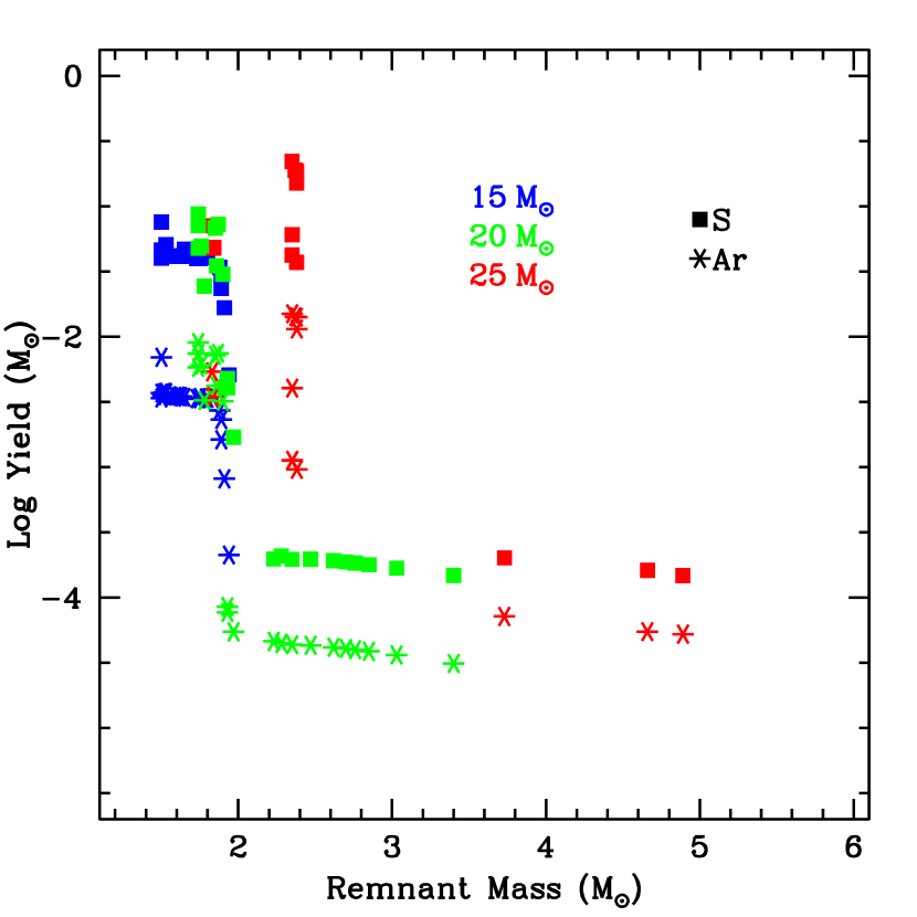
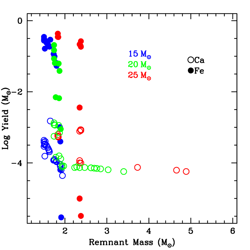
Figure 7.— Yields versus remnant mass for our 3 progenitors: $15\,M_{\odot}$ (blue), $20\,M_{\odot}$ (green), $25\,M_{\odot}$ (red). The four panels show all of the yields: upper left panel shows oxygen (open triangle) and neon (filled triangle), lower left panel shows magnesium (open square) and silicon (cross), upper right panel shows sulfar (filled square) and argon (star), and lower right panel shows calcium (open circle) and iron peak (filled circle). The precipitous drop in heavy element yields occurs at the top of the silicon shell. This shell is shocked to form the heavy elements. If none of this is ejected, we eject no heavy elements. Note, however, that if the explosion were asymmetric, it would be possible to eject some heavy elements at this remnant mass.

Figure 7 shows the yields from explosions versus compact remnant mass, color coded by the progenitor zero-age main sequence mass. Because the matter is not ejected, the yields decrease with increasing remnant mass, especially for the heavier elements. But there are noticeable deviations from this trend. First and foremost, because the shell burning layers have more mass in the larger progenitors, they can eject more mass, even when the remnant mass is larger. This is most evident in the $25\,M_{\odot}$ progenitor. For remnants less than $2.5\,M_{\odot}$, explosions of this progenitor can produce more mass of all the elements in our study. The effect of the supernova-induced nuclear burning is also evident in the range of yields for a given progenitor with the same final compact remnant mass. A strong impulse shock will produce more heavy elements than a slower, but continuously driven shock that drives an explosion, but prevents much fallback.

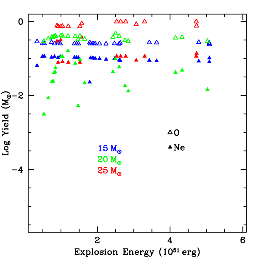
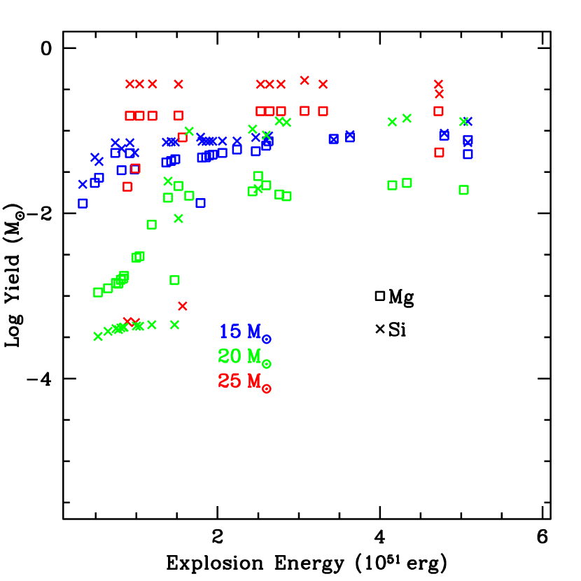
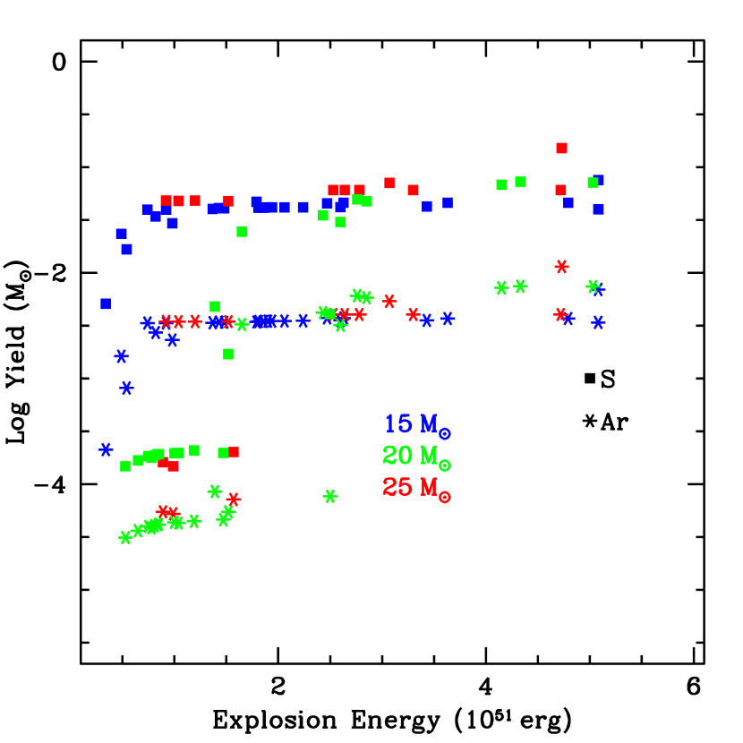
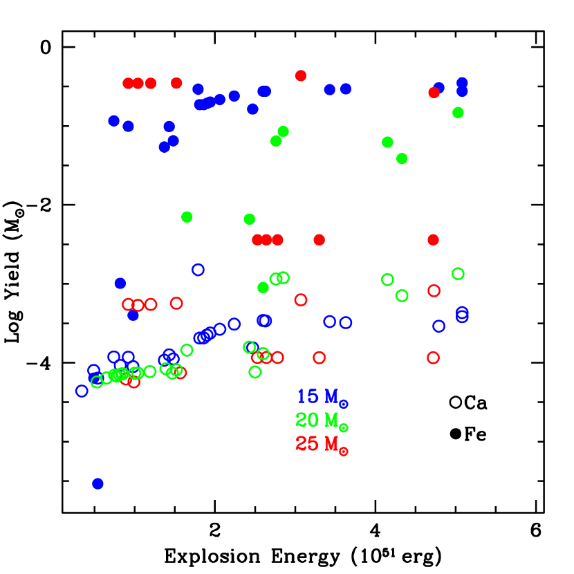
Figure 8.— Yields versus explosion energy for our 3 progenitors with the same color coding and symbols as figure 7.

To better see the dependence of the yields on the explosion energy, we plot the yields versus explosion energy (Fig. 8). At low energies, the primary effect on the yield is the amount of fallback. Stronger shocks (higher energy) have less fallback as most of the material is moving well over the escape velocity. But a continously driven explosion can have very little fallback even with an explosion of modest energy. But the shock also dictates the amount of shock-induced burning. Especially in the $15\,M_{\odot}$ progenitor where remnant masses do not change much for explosion energies above $10^{51}$ erg, the trends in explosion energy are more evident: neon and oxygen are typically destroyed in stronger explosions, but many of the other elements increase slightly.

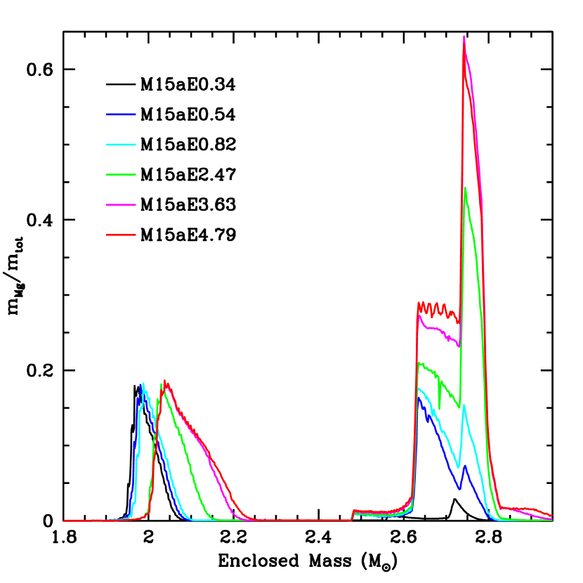
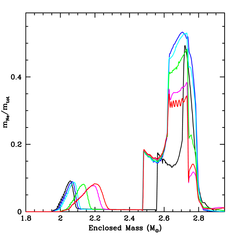
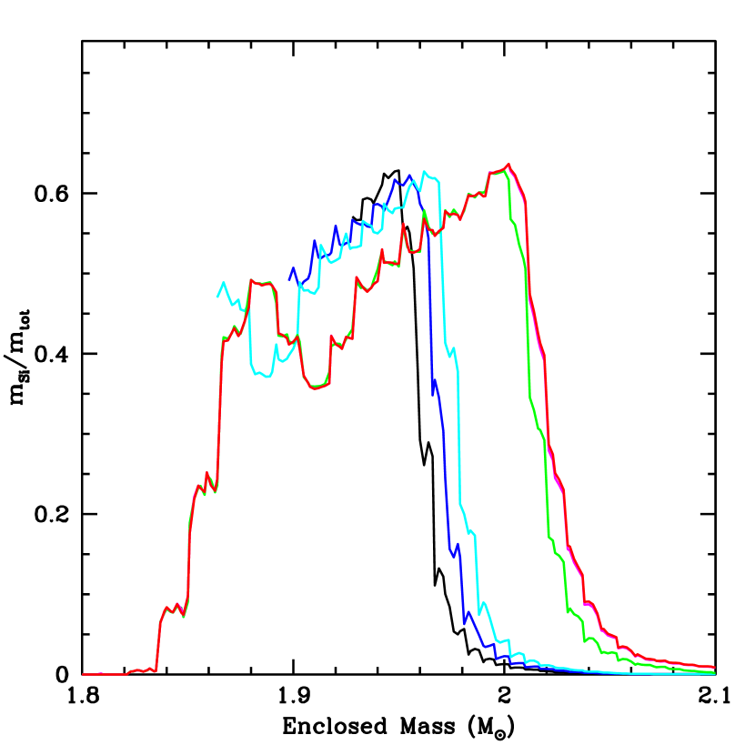
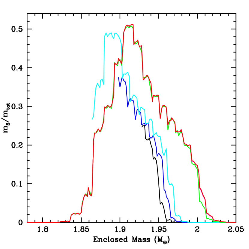
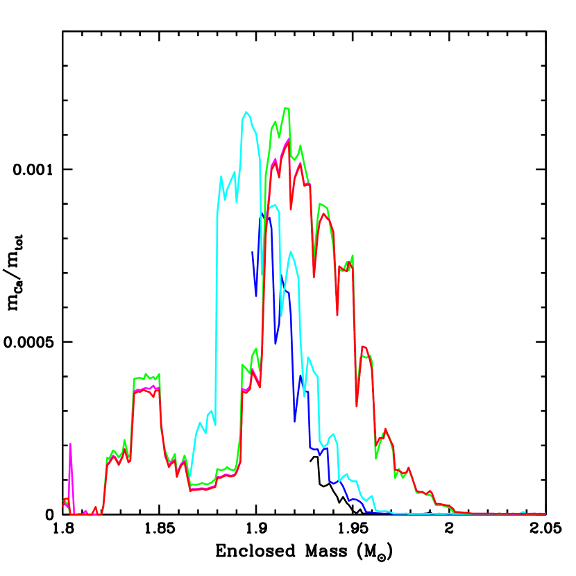
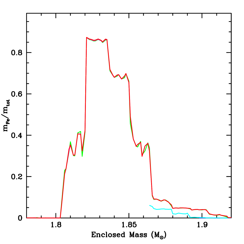
Figure 9.— Magnesium, neon, silicon, sulfur, calcium and iron abundances as a function of enclosed mass for the 15 M_⊙ a-series explosions: M15aE0.34 (black), M15aE0.58 (blue), M15aE0.82 (cyan), M15aE2.47 (green), M15aE3.63 (magenta), M15aE4.79 (red). In the lowest energy explosions, considerable material falls back, and those curves start at the innermost ejecta mass (below that start, the mass falls back).

The wide variation in abundances arises from a few basic trends in explosive nucleosynthesis: fallback and the production and destruction of elements in a supernova shock. For very weak explosions, material is not ejected with sufficient velocity and falls back onto the neutron star. The yield of the elements produced near the proto-neutron star is most affected by fallback. The iron yield is extremely sensitive to this fallback. Figure 9 shows the neon, magnesium, sulfur, calcium, silicon and iron abundances as a function of enclosed mass for the 15 M_⊙ progenitor with 6 explosion energies ranging from 0.34 to 4.79$\times 10^{51}$ erg. The iron abundance profile (abundance fraction as a function of enclosed mass) for the different-energy explosions is fairly similar, but the weak explosions simply don’t eject this mass. The silicon, sulfur, and calcium profiles are affected by fallback, but also by the shock strength. As the shock energy increases, it induces burning further out, producing more of these elements. Magnesium and neon demonstrate the third trend, the destruction of elements as they are fused into heavier elements. The abundance of neon initially increases with explosion energy, but then decreases as it is destroyed with the highest explosion energies. The combination of destruction and production make it difficult to predict trends in the final yields. The ratio of elements can be even more complex, producing the range of abundance ratios.

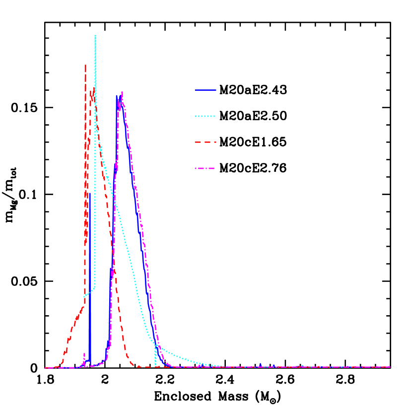
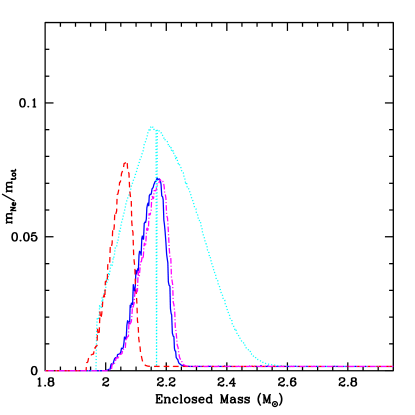
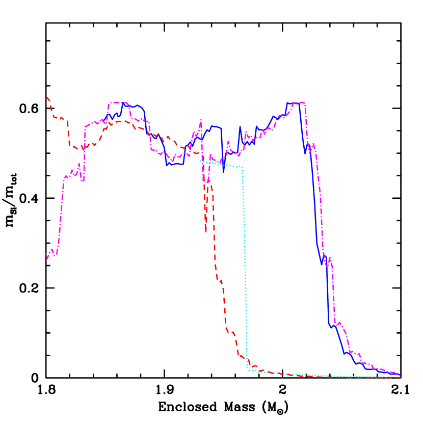
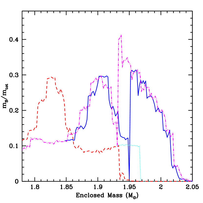
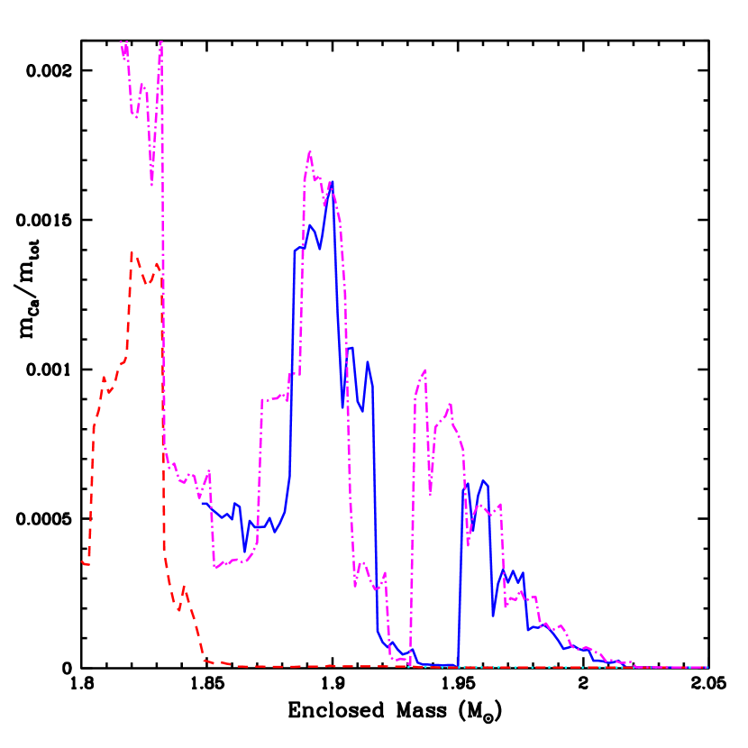
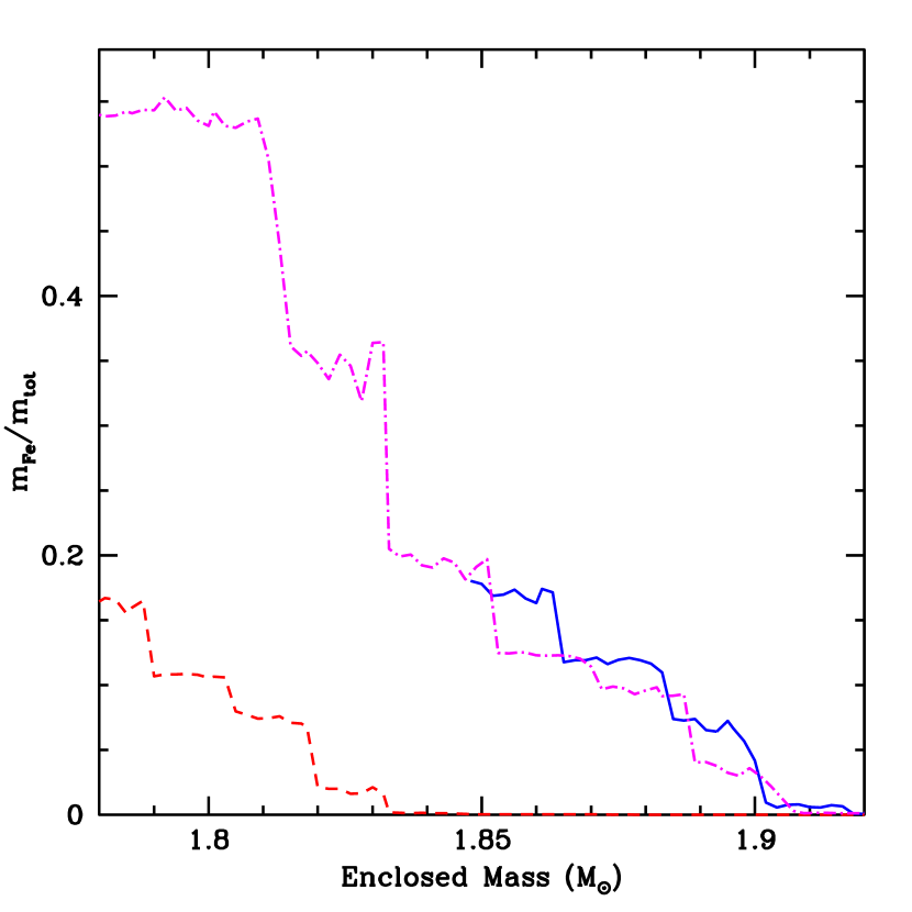
Figure 10.— Magnesium, neon, silicon, sulfur, calcium and iron abundances as a function of enclosed mass for four 20 M_⊙ explosions: M20aE2.43, M20aE2.50, M20cE1.65, M20cE2.76. Models M20aE2.43 and M20aE2.50 have nearly the same final explosion energy and the same total injection energy, but because energy injection occured on different time-frames. Models M20cE1.65 and M20cE2.76 have different initial core masses from the a-series models.

Additional complexities occur in the nature of the explosion. Figure 10 shows magnesium, neon, silicon, sulfur, calcium and iron abundances as a function of enclosed mass for four 20 M_⊙ explosions varying the injection time in the explosion and the core mass. Comparing two models with very similar injection and final energies, but different injection timescales, we see that the yields can vary dramatically. The longer injection timescale can change both the amount of fallback and the strength of the shock. Figure 10 also shows the differences between models using slightly different initial core masses. The different core masses reflect the time it takes for convection to become strong in the convective engine. If the growth time of the instability is long, more mass will accrete onto the proto-neutron star before the convective region robustly distributes energy across the convective region. The profiles, especially at higher mass coordinates, are not too different between models with different initial core masses. But the yields can be very different for elements, such as iron, that are produced in the innermost zones. Understanding the exact nature of the explosion is critical in determining the yields.

5. Conclusions

Within the paradigm of the convective engine we can produce a wide range of remnant masses and nucleosynthetic yields. Even so, some generic trends exist. First, even weak explosions are able to eject most of the star for the 15 M_⊙ star in this study because of its low binding energy (which is in agreement with most 15 M_⊙ stars). If an explosion occurs for such progenitors, the compact remnant is most likely going to be a neutron star. For more massive progenitors, late-time energy injection (either through fallback or magnetar-like activity) is required to make neutron star remnants with $10^{51}$ erg explosions. Without this late energy injection preventing fallback, more massive progenitors are likely to form black holes, even if $10^{51}$ erg explosion occurs. For the 25 M_⊙ progenitor, an explosion with energy less than $2\times 10^{51}$ erg without late-time energy injection will produce a black hole. If we assume the kick mechanism is produced by asymmetries in the ejecta, these systems are likely to be the ones that form kicks in black hole systems (Willems et al., 2005; Fragos et al., 2009).

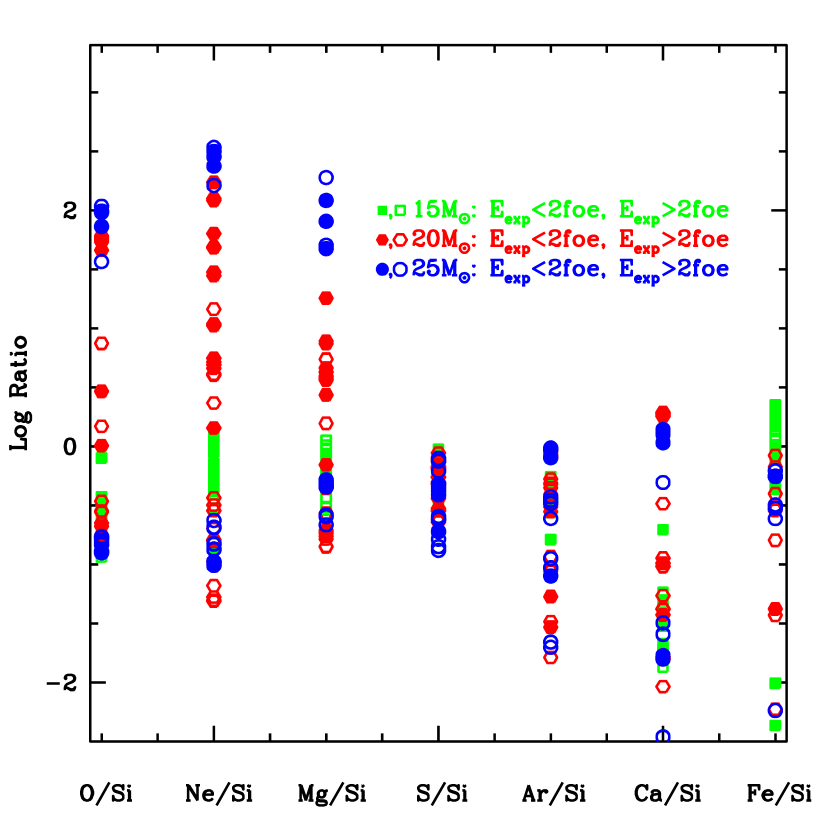
Figure 11.— Log ratio of a given element to Si with respect to solar abundances for a range of elements and all of our models: 15M_⊙ (circle), 20M_⊙ (triangle), 25M_⊙ (square). For the yield ratio, we can get a range of results. The solid symbols refer to explosion energies less than $2\times 10^{51}$ erg, open symbols refer to explosion energies above $2\times 10^{51}$ erg.

These abundances are inferred in the observations of a number of supernova remnants (e.g., Kumar et al., 2012) and abundance ratios have been used to place constraints on the supernova progenitor. Figure 11 shows the abundance ratio of a few key elements with respect to silicon: oxygen, neon, magnesium, sulfur, argon, calcium and iron peak. Each of our progenitors predict a range of yields based on the supernova explosion and in many cases, it will be difficult to discriminate the exact progenitor mass based on the yields. There are a few trends: more massive progenitors can produce more intermediate elements per silicon atom (oxygen, neon, magnesium) and less massive progenitors produce more iron elements vs. slicon. As we go up in mass beyond $25\,M_{\odot}$, stellar winds and mass-loss through binary interactions (e.g. a common envelope phase) can eject these intermediate elements. But if mass-loss is not strong, we expect these more massive stars to not produce supernovae, ejecting no heavy elements. Even these specific trends may be a particular characteristic of the progenitors we used (from the KEPLER (Weaver et al., 1978; Woosley et al., 2002; Heger & Woosley, 2010) code). The silicon shell is more massive in the recent TYCHO (Young et al., 2001) code progenitors, characteristic of the progenitors we used (from the KEPLER code). The silicon shell is more massive in the recent TYCHO code progenitors produced with modified mixing prescriptions (e.g., Arnett et al., 2010). More detailed studies of both progenitor and explosion yields will be required to truly understand the nucleosynthetic yields needed for discriminating supernova progenitors and in studying galactic chemical evolution.

With our parameterized study, we have found that the yields depend not only on the progenitor and final explosion energy, but on the nature of the explosion itself.

Acknowledgments This project was funded in part under the auspices of the U.S. Dept. of Energy, and supported by its contract W-7405-ENG-36 to Los Alamos National Laboratory. Simulations at LANL were performed on HPC resources provided under the Institutional Computing program. This research was supported in part by the National Science Foundation under Grant No. NSF PHY11-25915 and under LANL LDRD grant 20160173ER. The Joint Institute for Nuclear Astrophysics funded workshops that led to this research. The work of A.H. was supported by the Australian Research Council ARC FT120100363. The work of S.S.-H. was supported by NSERC (Natural Sciences and Engineering Research Council of Canada) and CSA (the Canadian Space Agency).

Table 1Remnant Masses

Model	Mprog	Mbounce	Minj	tinj	Einj	Eexp	Mremnant
	$(M_{\odot})$	$(M_{\odot})$	$(M_{\odot})$	s	$10^{51}$ erg	$10^{51}$ erg	$(M_{\odot})$
M15aE0.34	15	1.30	0.3	0.1	3	0.34	1.94
M15aE0.54	15	1.30	0.3	0.1	4	0.54	1.91
M15aE0.82	15	1.30	0.3	0.1	5	0.82	1.88
M15aE2.47	15	1.30	0.3	0.1	9	2.47	1.52
M15aE3.63	15	1.30	0.3	0.3	10	3.63	1.51
M15aE4.79	15	1.30	0.3	0.4	20	4.79	1.50
M15bE0.74	15	1.30	0.02	0.4	3	0.74	1.73
M15bE0.92	15	1.30	0.02	0.3	4	0.92	1.75
M15bE1.37	15	1.30	0.02	0.2	5	1.37	1.80
M15bE1.43	15	1.30	0.02	0.1	6	1.43	1.75
M15bE1.48	15	1.30	0.02	0.2	7	1.48	1.79
M15bE1.69	15	1.30	0.02	0.2	10	1.69	1.52
M15bE2.63	15	1.30	0.02	0.2	20	2.63	1.53
M15bE5.08	15	1.30	0.02	0.2	40	5.08	1.50
M15bE10.7	15	1.30	0.02	0.2	80	$>10.7$	1.53
M15cE0.49	15	1.30	0.1	0.4	3	0.49	1.89
M15cE0.98	15	1.30	0.1	0.4	5	0.98	1.89
M15cE1.79	15	1.30	0.1	0.4	7	1.79	1.65
M15cE1.81	15	1.30	0.1	0.4	8	1.81	1.63
M15cE1.86	15	1.30	0.1	0.3	9	1.86	1.63
M15cE1.90	15	1.30	0.1	0.3	10	1.90	1.62
M15cE1.94	15	1.30	0.1	0.3	12	1.94	1.61
M15cE2.06	15	1.30	0.1	0.3	15	2.06	1.59
M15cE2.24	15	1.30	0.1	0.3	25	2.24	1.56
M15cE2.60	15	1.30	0.1	0.3	45	2.60	1.52
M15cE3.43	15	1.30	0.1	0.3	90	3.43	1.51
M20aE0.53	20	1.56	0.1	0.50	4	0.53	3.40
M20aE0.65	20	1.56	0.1	0.12	4	0.65	3.03
M20aE0.81	20	1.56	0.1	0.12	7	0.81	2.70
M20aE0.85	20	1.56	0.1	0.50	7	0.85	2.62
M20aE1.39	20	1.56	0.1	0.12	10	1.39	1.93
M20aE1.47	20	1.56	0.1	0.50	10	1.47	2.23
M20aE2.43	20	1.56	0.1	0.12	20	2.43	1.86
M20aE2.50	20	1.56	0.1	0.50	20	2.50	1.93
M20aE4.15	20	1.56	0.1	0.12	50	4.15	1.85
M20bE0.78	20	1.56	0.2	0.12	5	0.78	2.85
M20bE1.04	20	1.56	0.2	0.12	6	1.04	2.47
M20bE1.19	20	1.56	0.2	0.12	8	1.19	2.28
M20bE1.52	20	1.56	0.2	0.12	10	1.52	1.97
M20bE2.60	20	1.56	0.2	0.12	25	2.60	1.90
M20bE4.33	20	1.56	0.2	0.12	50	4.33	1.87
M20cE0.75	20	1.47	0.1	0.5	6	0.75	2.76
M20cE0.84	20	1.47	0.1	0.5	7	0.84	2.62
M20cE1.00	20	1.47	0.1	0.5	8	1.00	2.35
M20cE1.65	20	1.47	0.1	0.5	10	1.65	1.78
M20cE2.76	20	1.47	0.1	0.5	15	2.76	1.76
M20cE2.85	20	1.47	0.1	0.5	20	2.85	1.74
M20cE5.03	20	1.47	0.1	0.5	50	5.03	1.74
M20cE8.86	20	1.47	0.1	0.5	100	8.86	1.74
M25aE0.99	25	1.83	0.1	0.1	5.0	0.99	4.89
M25aE1.57	25	1.83	0.1	0.1	10	1.57	3.73
M25aE4.73	25	1.83	0.1	0.1	20	4.73	2.38
M25aE6.17	25	1.83	0.1	0.1	35	6.17	2.38
M25aE7.42	25	1.83	0.1	0.1	50	7.42	2.37
M25aE14.8	25	1.83	0.1	0.1	100	14.8	2.35
M25bE0.76	25	1.83	0.02	0.3	4.0	0.76	5.54
M25bE1.86	25	1.83	0.02	0.5	6.0	1.86	3.52
M25bE1.92	25	1.83	0.02	1	8.0	1.92	3.13
M25bE8.40	25	1.83	0.02	0.28	50.0	8.40	2.38
M25bE9.73	25	1.83	0.02	0.69	100	9.73	2.35
M25bE18.4	25	1.83	0.02	0.69	200	18.4	2.35
M25d1E3.30	25	1.83	0.02	0.7,10-30	25	3.30	2.35
M25d1E4.72	25	1.83	0.02	0.7,10-30	50	4.72	2.35
M25d1E7.08	25	1.83	0.02	0.7,10-30	100	7.08	2.35
M25d2E2.53	25	1.83	0.02	0.7,100-300	20	2.53	2.35
M25d2E2.64	25	1.83	0.02	0.7,100-300	35	2.64	2.35
M25d2E2.78	25	1.83	0.02	0.7,100-300	50	2.78	2.35
M25d2E3.07	25	1.83	0.02	0.7,100-300	100	3.07	1.83
M25d3E0.89	25	1.83	0.02	0.7,1000-3000	7	0.89	4.66
M25d3E0.92	25	1.83	0.02	0.7,1000-3000	8	0.92	1.84
M25d3E1.04	25	1.83	0.02	0.7,1000-3000	10	1.04	1.84
M25d3E1.20	25	1.83	0.02	0.7,1000-3000	50	1.20	1.84
M25d3E1.52	25	1.83	0.02	0.7,1000-3000	100	1.52	1.83

Table 2Explosive Yields

Model	M${}_{O}(M_{\odot})$	M${}_{Ne}(M_{\odot})$	M${}_{Mg}(M_{\odot})$	M${}_{Si}(M_{\odot})$	M${}_{S}(M_{\odot})$	M${}_{Ar}(M_{\odot})$	M${}_{Ca}(M_{\odot})$	M${}_{Fe}(M_{\odot})$
M15aE0.34	0.29	0.064	0.013	0.022	0.0051	0.00021	$4.4\times 10^{-5}$	$5.5\times 10^{-8}$
M15aE0.58	0.25	0.11	0.027	0.043	0.017	0.00081	$6.4\times 10^{-5}$	$2.9\times 10^{-6}$
M15aE0.82	0.25	0.11	0.041	0.073	0.040	0.0033	$6.4\times 10^{-5}$	0.0010
M15aE2.47	0.25	0.098	0.057	0.083	0.045	0.0037	0.00015	0.16
M15aE3.63	0.27	0.086	0.083	0.089	0.046	0.0037	0.00032	0.29
M15aE4.79	0.27	0.0085	0.087	0.093	0.046	0.0037	0.00029	0.30
M15bE0.74	0.28	0.11	0.054	0.072	0.040	0.0033	0.00012	0.12
M15bE0.92	0.27	0.11	0.054	0.071	0.040	0.0033	0.00012	0.10
M15bE1.37	0.25	0.11	0.041	0.073	0.040	0.0034	0.00011	0.054
M15bE1.43	0.25	0.11	0.043	0.074	0.041	0.0034	0.00013	0.098
M15bE1.48	0.25	0.10	0.045	0.073	0.041	0.0034	0.00011	0.065
M15bE1.69	0.26	0.010	0.0052	0.072	0.040	0.0034	0.00039	0.27
M15bE2.63	0.26	0.0088	0.075	0.087	0.046	0.0037	0.00034	0.27
M15bE5.08	0.24	0.081	0.077	0.13	0.076	0.0069	0.00043	0.35
M15vE10.7	0.26	0.10	0.052	0.11	0.051	0.0037	0.00040	0.27
M15cE0.49	0.26	0.11	0.023	0.047	0.023	0.0016	$8.0\times 10^{-5}$	$6.4\times 10^{-5}$
M15cE0.98	0.25	0.11	0.034	0.054	0.030	0.0023	$8.9\times 10^{-5}$	0.00040
M15cE1.79	0.27	0.023	0.013	0.084	0.047	0.0034	0.0015	0.29
M15cE1.81	0.10	0.047	0.047	0.075	0.041	0.0035	0.00021	0.19
M15cE1.86	0.25	0.10	0.048	0.075	0.041	0.0035	0.00021	0.19
M15cE1.90	0.25	0.10	0.051	0.075	0.041	0.0035	0.00024	0.19
M15cE1.94	0.25	0.10	0.051	0.075	0.041	0.0035	0.00024	0.20
M15cE2.06	0.25	0.099	0.054	0.075	0.042	0.0035	0.00027	0.22
M15cE2.24	0.25	0.094	0.059	0.075	0.042	0.0035	0.00031	0.24
M15cE2.60	0.25	0.090	0.066	0.075	0.042	0.0035	0.00034	0.27
M15cE3.43	0.25	0.089	0.079	0.078	0.042	0.0035	0.00033	0.29
M20aE0.53	0.29	0.0031	0.0011	0.00032	0.00015	$3.1\times 10^{-5}$	$5.7\times 10^{-5}$	0.
M20aE0.65	0.34	0.0085	0.0012	0.00037	0.00017	$3.6\times 10^{-5}$	$6.4\times 10^{-5}$	0.
M20aE0.81	0.40	0.041	0.0016	0.00041	0.00019	$4.1\times 10^{-5}$	$7.1\times 10^{-5}$	0.0
M20aE0.85	0.40	0.056	0.0016	0.00045	0.00020	$4.1\times 10^{-5}$	$7.3\times 10^{-5}$	0.
M20aE1.39	0.40	0.073	0.015	0.025	0.0048	$8.5\times 10^{-5}$	$8.4\times 10^{-5}$	$3.8\times 10^{-7}$
M20aE1.47	0.33	0.0052	0.0016	0.00042	0.00020	$4.6\times 10^{-5}$	$7.4\times 10^{-5}$	0.
M20aE2.43	0.37	0.044	0.018	0.10	0.035	0.0042	0.00016	0.0066
M20aE2.50	0.50	0.070	0.037	0.092	0.018	0.00095	$7.8\times 10^{-5}$	$2.5\times 10^{-5}$
M20aE4.15	0.36	0.044	0.022	0.13	0.068	0.0072	0.0011	0.062
M20bE0.78	0.37	0.024	0.0014	0.00039	0.0018	$4.3\times 10^{-5}$	$7.4\times 10^{-5}$	0.
M20bE1.04	0.41	0.11	0.00030	0.00043	0.00020	$4.3\times 10^{-5}$	$7.4\times 10^{-5}$	0.
M20bE1.19	0.40	0.16	0.0073	0.00045	0.00021	$4.4\times 10^{-5}$	$7.7\times 10^{-5}$	0.
M20bE1.52	0.41	0.094	0.021	0.087	0.0017	$5.5\times 10^{-5}$	$8.1\times 10^{-5}$	$1.9\times 10^{-7}$
M20bE2.60	0.40	0.059	0.022	0.088	0.030	0.0032	0.00013	0.000089
M20bE4.33	0.37	0.048	0.023	0.14	0.073	0.0075	0.00071	0.039
M20cE0.75	0.38	0.024	0.0014	0.00040	0.00018	$4.0\times 10^{-5}$	$7.0\times 10^{-5}$	0.
M20cE0.84	0.40	0.043	0.0016	0.00042	0.00019	$4.1\times 10^{-5}$	$7.3\times 10^{-5}$	0.
M20cE1.00	0.42	0.11	0.0029	0.00043	0.00020	$4.3\times 10^{-5}$	$7.4\times 10^{-5}$	0.
M20cE1.65	0.33	0.022	0.016	0.099	0.024	0.0032	0.00014	0.0070
M20cE2.76	0.31	0.018	0.017	0.13	0.050	0.0061	0.0012	0.064
M20cE2.85	0.29	0.014	0.016	0.13	0.047	0.0058	0.0012	0.085
M20cE5.03	0.30	0.014	0.019	0.13	0.071	0.0074	0.0013	0.15
M20cE8.86	0.30	0.015	0.023	0.15	0.088	0.0090	0.00056	0.21
M25bE1.86	0.68	0.28	0.018	0.00039	0.00011	$5.2\times 10^{-5}$	$5.7\times 10^{-5}$	0.0
M25bE1.92	0.88	0.38	0.083	0.00076	0.00020	$7.1\times 10^{-5}$	$7.5\times 10^{-5}$	$4.0\times 10^{-9}$
M25bE8.40	1.05	0.13	0.19	0.41	0.037	0.00096	$9.9\times 10^{-5}$	$3.2\times 10^{-6}$
M25bE9.73	1.03	0.12	0.19	0.44	0.042	0.0011	0.00010	$1.0\times 10^{-5}$
M25bE18.4	1.04	0.12	0.19	0.43	0.042	0.0011	0.00010	$9.8\times 10^{-6}$
M25d1E3.30	0.99	0.11	0.17	0.37	0.061	0.0040	0.00012	0.0036
M25d1E4.72	0.99	0.11	0.17	0.37	0.061	0.0040	0.00012	0.0036
M25d1E7.08	0.99	0.11	0.17	0.37	0.061	0.0040	0.00012	0.0036
M25d2E2.53	0.99	0.11	0.17	0.37	0.061	0.0040	0.00012	0.0036
M25d2E2.64	0.99	0.11	0.17	0.37	0.061	0.0040	0.00012	0.0036
M25d2E2.78	0.99	0.11	0.17	0.37	0.061	0.0040	0.00012	0.0036
M25d2E3.07	0.84	0.090	0.17	0.41	0.072	0.0054	0.00063	0.43
M25d3E0.89	0.77	0.29	0.021	0.00049	0.00016	$5.5\times 10^{-5}$	$6.2\times 10^{-5}$	0.0
M25d3E0.92	0.73	0.078	0.15	0.37	0.048	0.0035	0.00055	0.35
M25d3E1.04	0.74	0.081	0.15	0.37	0.048	0.0034	0.00053	0.35
M25d3E1.20	0.73	0.078	0.15	0.37	0.048	0.0035	0.00055	0.35
M25d3E1.52	0.74	0.079	0.15	0.37	0.048	0.0034	0.00057	0.35

References

- Arnett et al. (2010) Arnett, D., Meakin, C., & Young, P. A. 2010, ApJ, 710, 1619
- Blinnikov et al. (1996) Blinnikov, S. I., Dunina-Barkovskaya, N. V., & Nadyozhin, D. K. 1996, ApJS, 106, 171
- Blondin et al. (2003) Blondin, J. M., Mezzacappa, A., & DeMarino, C. 2003, ApJ, 584, 971
- Burrows (2013) Burrows, A. 2013, Reviews of Modern Physics, 85, 245
- Burrows et al. (2016) Burrows, A., Vartanyan, D., Dolence, J. C., Skinner, M. A., & Radice, D. 2016, ArXiv e-prints
- Colgate (1971) Colgate, S. A. 1971, ApJ, 163, 221
- Couch & Ott (2015) Couch, S. M. & Ott, C. D. 2015, ApJ, 799, 5
- Ertl et al. (2016) Ertl, T., Janka, H.-T., Woosley, S. E., Sukhbold, T., & Ugliano, M. 2016, ApJ, 818, 124
- Fischer et al. (2010) Fischer, T., Whitehouse, S. C., Mezzacappa, A., Thielemann, F.-K., & Liebendörfer, M. 2010, A&A, 517, A80
- Fowler & Hoyle (1964) Fowler, W. A. & Hoyle, F. 1964, ApJS, 9, 201
- Fragos et al. (2009) Fragos, T., Willems, B., Kalogera, V., Ivanova, N., Rockefeller, G., Fryer, C. L., & Young, P. A. 2009, ApJ, 697, 1057
- Fröhlich et al. (2006) Fröhlich, C., Hauser, P., Liebendörfer, M., Martínez-Pinedo, G., Thielemann, F.-K., Bravo, E., Zinner, N. T., Hix, W. R., Langanke, K., Mezzacappa, A., & Nomoto, K. 2006, ApJ, 637, 415
- Fryer et al. (1999) Fryer, C., Benz, W., Herant, M., & Colgate, S. A. 1999, ApJ, 516, 892
- Fryer (1999) Fryer, C. L. 1999, ApJ, 522, 413
- Fryer (2006) —. 2006, New Astronomy Reviews, 50, 492
- Fryer (2009) —. 2009, ApJ, 699, 409
- Fryer et al. (2012) Fryer, C. L., Belczynski, K., Wiktorowicz, G., Dominik, M., Kalogera, V., & Holz, D. E. 2012, ApJ, 749, 91
- Fryer & Heger (2000) Fryer, C. L. & Heger, A. 2000, ApJ, 541, 1033
- Fryer & Kalogera (2001) Fryer, C. L. & Kalogera, V. 2001, ApJ, 554, 548
- Fryer & Young (2007) Fryer, C. L. & Young, P. A. 2007, ApJ, 659, 1438
- Grefenstette et al. (2017) Grefenstette, B. W., Fryer, C. L., Harrison, F. A., Boggs, S. E., DeLaney, T., Laming, J. M., Reynolds, S. P., Alexander, D. M., Barret, D., Christensen, F. E., Craig, W. W., Forster, K., Giommi, P., Hailey, C. J., Hornstrup, A., Kitaguchi, T., Koglin, J. E., Lopez, L., Mao, P. H., Madsen, K. K., Miyasaka, H., Mori, K., Perri, M., Pivovaroff, M. J., Puccetti, S., Rana, V., Stern, D., Westergaard, N. J., Wik, D. R., Zhang, W. W., & Zoglauer, A. 2017, ApJ, 834, 19
- Grefenstette et al. (2014) Grefenstette, B. W., Harrison, F. A., Boggs, S. E., Reynolds, S. P., Fryer, C. L., Madsen, K. K., Wik, D. R., Zoglauer, A., Ellinger, C. I., Alexander, D. M., An, H., Barret, D., Christensen, F. E., Craig, W. W., Forster, K., Giommi, P., Hailey, C. J., Hornstrup, A., Kaspi, V. M., Kitaguchi, T., Koglin, J. E., Mao, P. H., Miyasaka, H., Mori, K., Perri, M., Pivovaroff, M. J., Puccetti, S., Rana, V., Stern, D., Westergaard, N. J., & Zhang, W. W. 2014, Nature, 506, 339
- Grevesse & Noels (1993) Grevesse, N. & Noels, A. 1993, in Origin and Evolution of the Elements, ed. N. Prantzos, E. Vangioni-Flam, & M. Casse, 15–25
- Harris et al. (2017) Harris, J. A., Hix, W. R., Chertkow, M. A., Lee, C. T., Lentz, E. J., & Messer, O. E. B. 2017, ApJ, 843, 2
- Heger et al. (2003) Heger, A., Fryer, C. L., Woosley, S. E., Langer, N., & Hartmann, D. H. 2003, ApJ, 591, 288
- Heger & Woosley (2010) Heger, A. & Woosley, S. E. 2010, ApJ, 724, 341
- Heger et al. (2005) Heger, A., Woosley, S. E., & Spruit, H. C. 2005, ApJ, 626, 350
- Herant et al. (1994) Herant, M., Benz, W., Hix, W. R., Fryer, C. L., & Colgate, S. A. 1994, ApJ, 435, 339
- Houck & Chevalier (1992) Houck, J. C. & Chevalier, R. A. 1992, ApJ, 395, 592
- Hoyle et al. (1964) Hoyle, F., Fowler, W. A., Burbidge, G. R., & Burbidge, E. M. 1964, ApJ, 139, 909
- Ibeling & Heger (2013) Ibeling, D. & Heger, A. 2013, ApJ, 765, L43
- Jones et al. (2015) Jones, S., Hirschi, R., Pignatari, M., Heger, A., Georgy, C., Nishimura, N., Fryer, C., & Herwig, F. 2015, MNRAS, 447, 3115
- Kitaura et al. (2006) Kitaura, F. S., Janka, H.-T., & Hillebrandt, W. 2006, A&A, 450, 345
- Kumar et al. (2012) Kumar, H. S., Safi-Harb, S., & Gonzalez, M. E. 2012, ApJ, 754, 96
- Langer et al. (1983) Langer, N., Fricke, K. J., & Sugimoto, D. 1983, A&A, 126, 207
- Lattimer & Douglas Swesty (1991) Lattimer, J. M. & Douglas Swesty, F. 1991, Nuclear Physics A, 535, 331
- Lentz et al. (2015) Lentz, E. J., Bruenn, S. W., Hix, W. R., Mezzacappa, A., Messer, O. E. B., Endeve, E., Blondin, J. M., Harris, J. A., Marronetti, P., & Yakunin, K. N. 2015, ApJ, 807, L31
- Magkotsios et al. (2010) Magkotsios, G., Timmes, F. X., Hungerford, A. L., Fryer, C. L., Young, P. A., & Wiescher, M. 2010, ApJS, 191, 66
- Melson et al. (2015) Melson, T., Janka, H.-T., Bollig, R., Hanke, F., Marek, A., & Müller, B. 2015, ApJ, 808, L42
- Mönchmeyer & Müller (1989) Mönchmeyer, R. & Müller, E. 1989, in NATO Advanced Science Institutes (ASI) Series C, Vol. 262, NATO Advanced Science Institutes (ASI) Series C, ed. H. Ögelman & E. P. J. van den Heuvel, 549
- Müller et al. (2016a) Müller, B., Heger, A., Liptai, D., & Cameron, J. B. 2016a, MNRAS, 460, 742
- Müller et al. (2016b) Müller, B., Viallet, M., Heger, A., & Janka, H.-T. 2016b, ApJ, 833, 124
- O’Connor & Ott (2013) O’Connor, E. & Ott, C. D. 2013, ApJ, 762, 126
- Panov & Janka (2009) Panov, I. V. & Janka, H.-T. 2009, A&A, 494, 829
- Perego et al. (2015) Perego, A., Hempel, M., Fröhlich, C., Ebinger, K., Eichler, M., Casanova, J., Liebendörfer, M., & Thielemann, F.-K. 2015, ApJ, 806, 275
- Sukhbold et al. (2016) Sukhbold, T., Ertl, T., Woosley, S. E., Brown, J. M., & Janka, H.-T. 2016, ApJ, 821, 38
- Takiwaki et al. (2014) Takiwaki, T., Kotake, K., & Suwa, Y. 2014, ApJ, 786, 83
- Timmes et al. (2000) Timmes, F. X., Hoffman, R. D., & Woosley, S. E. 2000, ApJS, 129, 377
- Timmes et al. (1996) Timmes, F. X., Woosley, S. E., & Weaver, T. A. 1996, ApJ, 457, 834
- Ugliano et al. (2012) Ugliano, M., Janka, H.-T., Marek, A., & Arcones, A. 2012, ApJ, 757, 69
- Weaver et al. (1978) Weaver, T. A., Zimmerman, G. B., & Woosley, S. E. 1978, ApJ, 225, 1021
- Willems et al. (2005) Willems, B., Henninger, M., Levin, T., Ivanova, N., Kalogera, V., McGhee, K., Timmes, F. X., & Fryer, C. L. 2005, ApJ, 625, 324
- Woosley & Heger (2015) Woosley, S. E. & Heger, A. 2015, ApJ, 810, 34
- Woosley et al. (2002) Woosley, S. E., Heger, A., & Weaver, T. A. 2002, Reviews of Modern Physics, 74, 1015
- Young et al. (2001) Young, P. A., Mamajek, E. E., Arnett, D., & Liebert, J. 2001, ApJ, 556, 230