The magnetic field of molecular clouds

Abstract

The magnetic field of molecular clouds (MCs) plays an important role in the process of star formation: it determins the statistical properties of supersonic turbulence that controls the fragmentation of MCs, controls the angular momentum transport during the protostellar collapse, and affects the stability of circumstellar disks. In this work, we focus on the problem of the determination of the magnetic field strength. We review the idea that the MC turbulence is super-Alfvénic, and we argue that MCs are bound to be born super-Alfvénic. We show that this scenario is supported by results from a recent simulation of supernova-driven turbulence on a scale of 250 pc, where the turbulent cascade is resolved on a wide range of scales, including the interior of MCs.

1 The magnetic-field strength in MCs

The idea that MCs are magnetically supported against their gravitational collapse was reviewed in Shu et al. (1987). In that scenario, the observed random velocities correspond to MHD waves, or perturbations of a strong mean field. Gravitationally bound prestellar cores are initially subcritical and contract because of ambipolar drift until they become supercritical and collapse. Padoan & Nordlund (1997, 1999) proposed an alternative scenario where the mean magnetic field in MCs is weak and the observed turbulence is super-Alfvénic. By comparing results of two simulations, one with a weak field and the other with a strong field, with observational data, they showed that the super-Alfvénic case reproduced the observations better. Further results in support of the super-Alfvénic scenario were later presented in Padoan et al. (2004) and, more recently, by Lunttila et al. (2008, 2009) based on simulated Zeeman measurements.

In this review, we first address the super-Alfvénic nature of the turbulence in MCs in the context of their formation process. To support our scenario, we present results of a large-scale (250 pc) MHD simulation of interstellar medium (ISM) turbulence driven by supernova (SN) explosions. We then show that MC turbulence is super-Alfvénic also with respect to their rms magnetic field, amplified by the turbulence. Finally, we briefly summarize observational results in favor of this picture.

2 MCs are born super-Alfvénic

Different processes may contribute to the formation of MCs, and a full treatment of this problem should also address the mechanisms of conversion between atomic and molecular gas. For a general picture, we assume that MCs are the result of large-scale compressions of the warm interstellar medium (WISM), driven by the evolution of SN remnants. When such compressions reach the pressure threshold of the thermal instability, the compressed gas rapidly cools and compresses further to a characteristic density of MCs. We can characterize the large-scale turbulence of the WISM by its rms sonic and Alfvénic Mach numbers, $M_{\rm s}$ and $M_{\rm A}$. It is generally believed that the large-scale turbulence in the WISM is transonic and trans-Alfvénic, meaning $M_{\rm s}\sim 1$ and $M_{\rm A}\sim 1$.

Because of the transonic nature of the WISM turbulence, the large-scale velocity field can occasionally cause compressions strong enough to bring large regions above the thermal instability threshold. As the gas is further compressed thanks to its cooling, the magnetic field cannot be compressed because of the initially trans-Alfvénic nature of the flow, so the initial compression is forced to be primarily along the magnetic field direction. Assuming that turbulent velocities are not significantly decreased, the characteristic increase in density, $\rho_{\rm cold}\sim 100\,\rho_{\rm warm}$, results in a comparable increase in the turbulent kinetic energy, $E_{\rm K,cold}\sim 100\,E_{\rm K,warm}$, or a corresponding drop in the rms Alfvén velocity, $V_{\rm a,cold}\sim V_{\rm a,warm}/10$. As a consequence, the turbulence in the rapidly cooling gas must be initially super-Alfvénic with respect to the mean magnetic field (Nordlund & Padoan, 2003; Padoan et al., 2010). Compression and stretching in this super-Alfvénic flow can then locally amplify the magnetic field, without affecting the mean field. Because of the reduced temperature, the turbulence in the cold gas is also supersonic, so dense cores with enhanced magnetic field strength are naturally formed by shocks in the turbulent flow. This sequence of events is schematically depicted in Fig. 1.

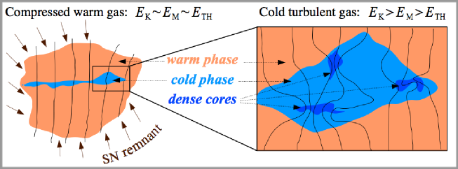
Figure 1: Schematic scenario of the formation of super-Alfvénic MCs.

3 Supernova-driven turbulence

The above scenario of MC formation is supported by a recent SN-driven MHD simulation (Padoan et al., 2016b; Pan et al., 2016; Padoan et al., 2016a, 2017) that models a 250-pc ISM region, large enough to address the formation and evolution and MCs. The MHD equations are solved with the Ramses AMR code (Teyssier, 2002; Fromang et al., 2006; Teyssier, 2007) within a cubic region of size $L_{\rm box}=250$ pc, total mass $M_{\rm box}=1.9\times 10^{6}$ $M_{\odot}$, and periodic boundary conditions. The mean density is $n_{\rm H,0}=5$ cm^-3 and the mean magnetic field $B_{0}=4.6$ $\mu$G. The rms magnetic field amplified by the turbulence is 7.2 $\mu$G.

The only driving force is from SN feedback. SNe are randomly distributed in space and time during the first period of the simulation without self-gravity, while they are later determined by the position and age of the massive sink particles formed when self-gravity is included. In the initial phase without gravity, the minimum cell size is $dx=0.24$ pc until $t=45$ Myr. It is then decreased to $dx=0.03$ pc, using a root-grid of $512^{3}$ cells and four AMR levels, during an additional period of 10.5 Myr without self-gravity. Finally, at $t=55.5$ Myr, gravity is introduced and the minimum cell size is further reduced to $dx=0.0076$ pc by adding two more AMR levels.

To follow the collapse of prestellar cores, sink particles are created in cells where the gas density is larger than $10^{6}$ cm^-3 if a number of conditions are met (see Haugbølle et al., 2017). When a sink particle of mass larger than 7.5 M_⊙ has an age equal to the corresponding stellar lifetime for that mass, a sphere of $10^{51}$ erg of thermal energy is injected at the location of the sink particle to simulate the SN explosion, as described in detail in Padoan et al. (2016b). We refer to this driving method as real SNe, as it provides a SN feedback that is fully consistent with the star-formation rate (SFR), the stellar initial mass function, and the ages and positions of the individual stars whose formation is resolved in the simulation. The simulation has so far been run for approximately 30 Myr with self-gravity, star formation and real SNe, generating over 7000 stars and hundreds of MCs. The SFR in the MCs has realistic values, while the global SFR corresponds to a mean gas-depletion time in the computational volume of almost 1 Gyr, also realistic for a 250-pc scale (Padoan et al., 2017).

4 The mean and rms magnetic-field strength of MCs

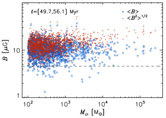
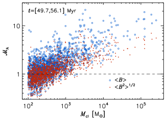
Figure 2: Left: Magnetic field strength versus cloud mass for a sample of 1,547 MCs selected from our SN-driven simulation. The dashed line shows the mean magnetic field averaged over the whole computation volume (also the initial mean field). Empty circles correspond to the mean value of the magnetic field of all tracer particles in each cloud, while filled circles give the rms value. Right: Alfvénic rms Mach number versus cloud mass for the same clouds as in the left panel, computed with the cloud mean magnetic field (empty circles), or the cloud rms magnetic field (filled cirlces).

The simulation adopts a mean magnetic-field strength consistent with the Galactic one, so the magnetic field inside clouds selected from the simulation should be comparable to that in real MCs. To investigate the role of the magnetic field in individual MCs, in Padoan et al. (2016b) we consider a catalog of 1,547 clouds selected from several snapshots of the simulation, based on a density threshold of $n_{\rm H,min}=200$ cm^-3. The mean and rms magnetic field of each cloud is computed using the values sampled by tracer particles embedded in the simulation, $\langle B\rangle=\Sigma_{\rm i}B_{\rm i}/N$ and $\langle B^{2}\rangle^{1/2}=(\Sigma_{\rm i}B^{2}_{\rm i}/N)^{1/2}$, where $B_{\rm i}$ is the magnetic field strength sampled by the particle i in a given cloud, and $N$ is the total number of particles in that cloud. These magnetic field values are plotted versus the cloud mass in the left panel of Fig. 2, where the horizontal dashed line represents the mean magnetic field in the computational volume, $B_{0}=4.6$ $\mu$G.

The mean field in the clouds (empty circles) is approximately 10 $\mu$G on average, only twice larger than the large-scale magnetic-field strength, $B_{0}$, and independent of cloud mass. We have verified that the mean magnetic-field strength of the clouds is also independent of their mean gas density. The relatively small increase of the cloud mean magnetic field relative to $B_{0}$ and its independence of gas density are characteristic of trans-Alfvénic supersonic turbulence (Padoan & Nordlund, 1997, 1999), and illustrates that MCs must be formed by compressive motions primarily along magnetic field lines, due to the non-negligible magnetic pressure prior to the compression and cooling of the low-density gas, as discussed above.

Because in super-Alfvénic turbulence the magnetic field is amplified by compressions, as shown by a positive $B-n$ correlation (Padoan & Nordlund, 1997, 1999), our scenario also predicts the formation of dense cores, formed by shocks within MCs (Padoan et al., 2001), with an enhanced magnetic-field strength. The small-scale enhancement of the magnetic field within MCs is illustrated in the left panel of Fig. 2, where the values of the rms field in the clouds (filled circles) is approximately a factor of two larger than the mean field. The rms field increases slightly with cloud mass, due to the correlation between rms velocity and cloud mass: Larger, more massive clouds have larger rms velocity than smaller clouds, on average, so the rms field is amplified to a larger value.

As a more direct demonstration of the super-Alfvénic nature of MC turbulence, the right panel of Fig. 2 shows the cloud rms Alfvénic Mach number versus the cloud mass. The Mach number is computed as the ratio of the cloud rms velocity and the cloud Alfvén velocity, where the latter is computed either with the mean magnetic field (empty circles) or with the rms magnetic field (filled circles), and using the mean density sampled by the tracer particles. Nearly all clouds with mass larger than $10^{3}$ M_⊙ are super-Alfvénic, even considering their amplified field strength. For the 41 MCs with masses larger than $10^{4}$ M_⊙, the average Alfvénic Mach number is 8.3 with respect to the mean field, and 3.9 with respect to the rms field.

The inability of supersonic turbulence to amplify the magnetic field to equipartition with the kinetic energy, as in the MCs of our simulation, was already established with idealized simulations of randomly-driven MHD turbulence. Simulations by Haugen et al. (2004) suggested that the growth rate of the turbulent dynamo in the supersonic regime may be significantly reduced compared to the incompressible case. Later on, simulations with rms sonic Mach number ${\mathcal{M}}_{\rm s}\approx 10$ and different values of the rms Alfvénic Mach number, ${\mathcal{M}}_{\rm A}\approx 30$, 10, and 3 (Kritsuk et al., 2009b, a; Padoan et al., 2010), also showed that the saturated rms magnetic field is a function of the mean field, and it is consistent with amplification by compression, with no contribution from a turbulent dynamo (see eq. (20) in Padoan & Nordlund, 2011). As firmly established in the comprehensive parameter study by Federrath et al. (2011), a supersonic turbulent dynamo plays a role in the field amplification only when the mean magnetic field is very small, as the saturated value of the magnetic energy is only a few percent of the kinetic energy.

Equation (20) in Padoan & Nordlund (2011) corresponds to the following relation between the rms Alfvénic Mach number computed with the rms magnetic field, ${\mathcal{M}}_{\rm A,rms}$, and the ratio of Alfvénic to sonic Mach numbers based on the mean magnetic field, ${\mathcal{M}}_{\rm A}$ and ${\mathcal{M}}_{\rm s}$ respectively:

$${\mathcal{M}}_{\rm A,rms}\sim({\mathcal{M}}_{\rm A}/{\mathcal{M}}_{\rm s})^{1/2}.$$ (1)

This predicted saturation level is shown by the long-dashed line in fig. 3. One can see that it defines the lower envelope of the scatter plot of ${\mathcal{M}}_{\rm A,rms}$ versus ${\mathcal{M}}_{\rm A}$ for the MCs selected from our SN-driven simulation. Many clouds are found well above the saturation level, which may be due to their relatively young age, or to an insufficient numerical resolution in the case of the smallest clouds.

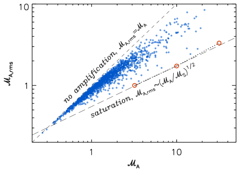
Figure 3: The rms Alfvénic Mach number computed with the rms magnetic field, ${\mathcal{M}}_{\rm A,rms}$, versus the Alfvénic Mach number based on the mean magnetic field, ${\mathcal{M}}_{\rm A}$, for the same MCs selected from the SN-driven simulation as in fig. 2. The long-dashed line shows the saturation value from eq. (1), while the open circles indicate the saturation values from randomly driven simulations (Kritsuk et al., 2009b, a; Padoan et al., 2010).

5 Comparison with Observations

The super-Alfvénic nature of the turbulence in the clouds from our simulation is consistent with the observational evidence. Based on the comparison between simulations of MHD turbulence and MC observations, Padoan & Nordlund (1997, 1999) suggested that MC turbulence was better characterized by supersonic turbulent flows with ${\mathcal{M}}_{A}\gg 1$ than flows with ${\mathcal{M}}_{A}\approx 1$. This result was later confirmed with the aid of synthetic observations (Padoan et al., 2004) and synthetic Zeeman splitting measurements (Lunttila et al., 2008). It was shown that a super-Alfvénic turbulence simulation with the characteristic size, density, and velocity dispersion of star-forming regions could produce dense cores with the same relation between magnetic-field strength and column density as observed cores. Lunttila et al. (2008) also computed the relative mass-to-flux ratio ${\mathcal{R}}_{\mu}$, defined as the mass-to-flux ratio of a core divided by that of its envelope, as proposed by Crutcher et al. (2009). They found a large scatter in the value of ${\mathcal{R}}_{\mu}$, and an average value of ${\mathcal{R}}_{\mu}<1$, in contrast to the ambipolar-drift model of core formation, where the mean magnetic field is stronger and only ${\mathcal{R}}_{\mu}>1$ is allowed. Crutcher et al. (2009) confirmed that ${\mathcal{R}}_{\mu}<1$ in observed cores, as predicted by Lunttila et al. (2008).

In a separate work, Lunttila et al. (2009) used simulated OH Zeeman measurements to compute the mass-to-flux ratio relative to the critical one, $\lambda$, and the ratio of turbulent to magnetic energies, $\beta_{\rm turb}$, in molecular cores selected from a super-Alfvénic simulation. They found both mean values and scatter of $\lambda$ and $\beta_{\rm turb}$ in good agreement with the observational results of Troland & Crutcher (2008). In our super-Alfvénic scenario, the scatter originates partly from intrinsic variations of the magnetic field strength from core to core, which are not expected in the traditional picture of MCs were the mean magnetic field is strong (Shu et al., 1987).

Taking advantage of the anisotropy of MHD turbulence, Heyer & Brunt (2012) demonstrated that the densest regions of the Taurus MC complex are characterized by super-Alfvénic turbulence, while in low density regions the motions are sub or trans-Alfvénic, also consistent with the picture from our simulation, where MCs are formed by large-scale trans-Alfvénic turbulence, and thus fed preferentially by motions along magnetic field lines, as discussed above (Nordlund & Padoan, 2003; Padoan et al., 2010). Recent dust polarization measurements have shown that the magnetic field has a relatively constant orientation in low-density regions surrounding MCs, with the mean direction mainly parallel to low-density filaments, while the field becomes predominantly perpendicular to the direction of dense filaments in regions of larger column density (Soler et al., 2017). This change is suggestive of the transition from trans-Alfvénic to super-Alfvénic turbulence found by Heyer & Brunt (2012).

6 Conclusions

We have argued that MCs are born super-Alfvénic with respect to their mean magnetic field, because of the trans-Alfvénic nature of the turbulence in the WISM. We have shown that this scenario is supported by the results of a SN-driven simulation meant to represent an overdense region (e.g. a spiral arm) of the ISM on a scale of 250 pc, with a realistic mean magnetic field. MCs selected from the simulation have a mean magnetic-field strength of approximately 10 $\mu$G, only a factor of two larger than the mean field averaged over the whole computational volume. Their internal rms velocity is super-Alfvénic with respect to both their mean and rms magnetic field strength.

Despite the small value of their mean magnetic field strength, super-Alfvénic MCs are expected to naturally generate dense cores with stronger magnetic field as the result of compression by turbulent shocks. The properties of such cores measured in simulations of super-Alfvénic turbulence are consistent with those of real MC cores.