Weakly nonergodic dynamics in the Gross–Pitaevskii lattice

Abstract

The microcanonical Gross–Pitaevskii (aka semiclassical Bose-Hubbard) lattice model dynamics is characterized by a pair of energy and norm densities. The grand canonical Gibbs distribution fails to describe a part of the density space, due to the boundedness of its kinetic energy spectrum. We define Poincare equilibrium manifolds and compute the statistics of microcanonical excursion times off them. The tails of the distribution functions quantify the proximity of the many-body dynamics to a weakly-nonergodic phase, which occurs when the average excursion time is infinite. We find that a crossover to weakly-nonergodic dynamics takes place inside the nonGibbs phase, being unnoticed by the largest Lyapunov exponent. In the ergodic part of the non-Gibbs phase, the Gibbs distribution should be replaced by an unknown modified one. We relate our findings to the corresponding integrable limit, close to which the actions are interacting through a short range coupling network.

Equipartition and thermalization are cornerstone concepts of understanding stability and predictability of complex matter dynamics. Proximity to integrable limits may have a strong impact on the needed time scales, or even on equipartition itself. Let us consider a dynamical system which is characterized by a countable set of preserved actions at the very integrable limit, as e.g. for harmonic lattice vibrations in crystals. Close to the limit, nonintegrable couplings between the actions induce a nontrivial dynamics of the latter. The nonintegrable couplings define a certain connectivity network on the action lattice.

The nonlinear coupling network of the actions can be long ranged. That is precisely the case with translationally invariant weakly nonlinear lattice wave equations, or phonon dynamics in crystals, or e.g. the celebrated Fermi-Pasta-Ulam (FPU) chain Fermi et al. (1955); Ford (1992). Then the linear integrable limit yields actions which are related to standing or plane waves (harmonic phonons) which traverse the entire system. Weak local nonlinearities therefore induce a coupling network which is long ranged Ford (1992). At whatever small, but finite, energy densities in an equipartitioned state, all plane waves and thus actions will be coupled regardless of their characteristics (e.g. the eigenfrequency). Selection rules due to momentum conservation do not alter the above argument. Nature nicely confirms that, since phonon dynamics in crystals appears to be equipartitioned down to the smallest temperatures. At the same time, approaching zero densities will lead to a diminishing of the largest Lyapunov exponent, and thus equipartition times are expected to smoothly diverge in the very limit.

The focus of this work is the case of a Gross–Pitaevskii (GP), aka Bose-Hubbard (BH), lattice with local nonlinear many-body interactions, and short range hoppings. In the limit of large densities the nonlinear interactions dominate over the hoppings, the actions turn local in real space, and the system disintegrates into an uncoupled set of strongly anharmonic oscillators in real space. Close to the limit the short range hoppings induce a nonintegrable short range coupling network between the actions. Anomalous and potentially nonergodic large density dynamics was reported for the GP lattice Rasmussen et al. (2000); Rumpf (2004, 2008, 2009), including nonequilibrium transport properties Iubini et al. (2012, 2013) and self localization Livi et al. (2006); Hennig and Fleischmann (2013); Kruse and Fleischmann (2017). Indications for nonergodic dynamics were also observed for similar model classes Ivanchenko et al. (2004); Pino et al. (2016).

Strict nonergodic dynamics implies a separation of the phase space into disjoint parts under the action of Hamiltonian dynamics, which could imply the presence of additional symmetries. Such symmetries are unlikely to be restored upon the smooth change of control parameters. An alternative scenario is observed in glassy dynamics, as e.g. shown by Bouchaud via the appearance of consecutive metastable states, whose lifetimes are distributed according to power-law distributions Bouchaud (1992). If the average lifetime of the metastable states turns infinite, a trajectory might still visit almost all the phase space, however strictly infinitely long time is required to observe that when computing averages. Such dynamics, while formally being ergodic, turns nonergodic for any finite averaging time. Similar behavior has been discussed by Eli, Rebenshtok and Barkai in a set of papers dedicated to continuous-time random walks Bel and Barkai (2005, 2006); Rebenshtok and Barkai (2007). Therein, the phenomenon goes under the name of weak ergodicity breaking, or weak nonergodicity. Lutz further formalized the connection between power-law distribution and weak nonergodicity in the context of optical lattices Lutz (2004).

The goal of this work is to show the existence of a weak nonergodic phase of the GP lattice dynamics and to quantitatively assess the crossover line from an ergodic to a weak nonergodic regime in the relevant two-dimensional density parameter space. The GP lattice dynamics is conserving energy and norm (particle number). The microcanonical dynamics is depending on the corresponding pair of densities. If the dynamics is ergodic, the time average of an observable (a function of the phase space coordinates) should exist and be equal to a phase space average with a proper distribution function. Assuming equal weight of microstates, the Boltzmann (canonical) or Gibbs (grand canonical) distributions are the proper choice. Rasmussen et al. showed that the Gibbs distribution with positive temperature and arbitrary chemical potential is addressing only a part of the accessible microcanonical density space Rasmussen et al. (2000). Negative temperatures yield divergent partition functions, and a proper nonGibbs distribution for the complementary space is not known. In that nonGibbs density space the microcanonical dynamics is characterized by anomalous fluctuations, slow relaxations, and potentially (weakly) nonergodic dynamics. We note that the mere fact of a nonGibbs regime is not sufficient to conclude that the dynamics is nonergodic, since the analysis is based solely on phase space integrations and does not consider any aspect of the accompanying dynamics.

Our strategy is to use proper observables $f$ as functions of the phase space variables. Assuming ergodicity we may obtain the expected phase space average $\bar{f}$. The condition $f=\bar{f}$ defines an equilibrium Poincare manifold of co-dimension 1 which separates the accessible microcanonical phase space into two disjoint sets. By assumption of ergodicity, a microcanonical trajectory must pierce this manifold infinitely many times during its evolution, to ensure that the microcanonical time average $\langle f\rangle=\bar{f}$. Let us consider the event of two consecutive piercings, and the trajectory excursion off the manifold in between. We will assess the statistics, correlations, and other properties of these excursions. At variance with correlation function computations, our strategy allows to return to individual excursions which contribute to a particular feature. In a recent study Danieli et al. (2017) of a finite FPU system, an entropy function on the system phase space was used as an observable $f$. This integral quantity becomes insensitive to relevant nonergodic fluctuations in the limit of large volume $N$. The key ingredient in this work is to use simultaneously all observables which correspond to integrals of motion in the large density limit. The piercings of one single trajectory through $N$ equilibrium manifolds will then be analyzed.

The one-dimensional GP lattice equations read

$$i\frac{\partial\psi_{m}}{\partial t}+(\psi_{m+1}+\psi_{m-1})-g|\psi_{m}|^{2}\psi_{m}=0,$$ (1)

where $m$ labels the lattice sites, and $g$ is a nonlinear parameter related to the two-body scattering length. Eq.(1) is generated by the Hamiltonian equations of motion $i\dot{\psi}_{m}=\frac{\partial\mathcal{H}}{\partial\psi_{m}^{\ast}}$ with the Hamiltonian

$$\mathcal{H}=\sum_{m}\big{[}-(\psi_{m}^{\ast}\psi_{m+1}+\psi_{m}\psi_{m+1}^{\ast})+\frac{g}{2}|\psi_{m}|^{4}\big{]}.$$ (2)

Here $\psi_{m}^{\ast}$ and $\psi_{m}$ are pairs of conjugated phase space variables, the sum runs over $N$ lattice sites, and periodic boundary conditions $\psi_{1}=\psi_{N+1}$ are used. In addition to the total energy $\mathcal{H}$, the above equations also conserve the norm $\mathcal{A}=\sum_{m}|\psi_{m}|^{2}$ which is the classical analogue to the quantum mechanical total number of particles. The canonical transformation $\psi_{m}=\sqrt{A_{m}}\exp(i\phi_{m})$ maps Eq.(2) into

$$\mathcal{H}=\sum_{m}\big{[}-2\sqrt{A_{m}A_{m+1}}\cos(\phi_{m}-\phi_{m+1})+\frac{g}{2}|A_{m}|^{2}\big{]}.$$ (3)

Rasmussen et al. Rasmussen et al. (2000) used Eq.(3) to compute the classical grand-canonical partition function

$$\textit{Z}=\int_{0}^{\infty}\int_{0}^{2\pi}\prod_{m=1}^{N}d\phi_{m}dA_{m}\exp^{-\beta(\mathcal{H}+\mu\mathcal{A})}.$$ (4)

Here $\mu$ is the chemical potential and $\beta$ the inverse temperature $\beta=1/T\geq 0$. The mapping of the pair of Gibbs parameters $\{\beta,\mu\}$ onto the microcanonical density space $\{h,a\}$ with $h=\mathcal{H}/N$ and $a=\mathcal{A}/N$ leaves a part of the high energy density space unaddressed, with the infinite temperature $\beta=0,\beta\mu=const$ line being the border between the addressable density space part (Gibbs regime) and the complementary one (nonGibbs regime) Rasmussen et al. (2000). It is convenient to use rescaled densities $x=ga$, $y=gh$. Then the Gibbs part of the density space is sandwiched between the zero temperature $\beta=\infty$ line $y_{GS}=-2x+x^{2}/2$ and the infinite temperature $\beta=0$ one $y_{nG}=x^{2}$ in Fig.1.

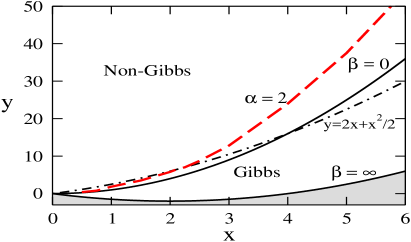
Figure 1: (Color online) GP phase diagram in the microcanonical density space $(x,y)$. Thick solid lines $y_{GS}=-2x+x^{2}/2$ and $y_{nG}=x^{2}$ are for $\beta=\infty$ ($T=0$) and $\beta=0$ ($T=\infty$), respectively. No microcanonical states exist below the $\beta=\infty$ line and this area is shaded. Microcanonical states above the $\beta=0$ line exist, but are not addressable through a Gibbs distribution. Dashed-dotted line $y_{h}=2x+x^{2}/2$, above which microcanonical states with constant norm density $|\psi_{m}|=const$ cease to exist. Thick dashed line (red): ergodic to nonergodic transition dynamics where $\alpha=2$ (see text for details).

It was conjectured that microcanonical dynamics in the nonGibbs phase is nonergodic due to the observed formation of concentrated hot spots of localized norm/energy excitations Rasmussen et al. (2000). These excitations appear to be related to exact discrete breather solutions Flach and Willis (1998); Campbell et al. (2004); Flach and Gorbach (2008); Franzosi et al. (2011). Interestingly these exact finite energy time-periodic solutions are continuable into single site anharmonic oscillator excitations in the integrable limit of infinite densities, coined anticontinuous limit by MacKay and Aubry MacKay and Aubry (1994). Rumpf developed an entropic picture of fragmentation of the field into two components in the nonGibbs regime - a condensate of the above hot spots, and a remaining thermalized component with infinite temperature $\beta=0$ Rumpf (2004, 2008). Whether the spots thermalize and whether the system is ergodic or not, remained unaddressed. This leads to the question, whether the GP lattice turns nonergodic precisely in the nonGibbs regime. Below we will study lifetime distributions of the hot spots, show that these times stay finite inside a part of the nonGibbs regime, and discuss the consequences. We also note that homogeneous norm density states $\psi_{m}=\sqrt{a}e^{i\phi_{m}}$ with $\phi_{m}=0$ minimize the energy at a given value of $x$ and yield the $\beta=\infty$ line. At the same time, the largest energy of these states is obtained for $\phi_{m}=\pi$ and yields the line $y_{h}=2x+x^{2}/2$, which is located in the nonGibbs regime for $x\leq 4$ in Fig.1. Thus nonGibbs dynamics can be generated with initial states which are completely homogeneous in their norm and energy density distributions. For energy densities $y>y_{h}$ no homogeneous states are available.

In all simulations shown in this work, Eq.(1) is integrated by using the symplectic procedure $SBAB_{2}$ described in Ref.Skokos et al. (2009), with time step $\Delta t=0.02$, which keeps the relative energy error below $0.1\%$ (the total norm is conserved up to computational roundoff precision). The observables are simply the local norm densities $f_{n}=g|\psi_{n}|^{2}$, $n=1,...,N$ which turn into integrals of motion in the infinite density limit. They define $N$ ergodic Poincaré sections $\mathcal{F}_{n}:f_{n}=x$. Unless specified otherwise, we consider $N=2^{10}$ sites. We integrate a trajectory and track the times $t_{i}^{(n)}$ the trajectory pierces any of the equilibrium manifolds $\mathcal{F}_{n}$. The excursion times follow as $\tau^{(n,\pm)}(i)=t^{(n)}_{i+1}-t_{i}^{(n)}$ where the sign $\pm$ is set by the sign of $(f_{n}-x)$ during the excursion and tells whether we monitor an excursion with local augmentation (+) or depletion (-) of the norm density. We then obtain the probability distribution functions (PDF) of the excursion times $P_{\pm}(\tau)$. We attempt to fit the PDF tails with a power law $P(\tau)\propto\tau^{-\alpha}$ to find the dependence of $\alpha$ on the densities $(x,y)$. For $\alpha\leq 2$ we conclude that the dynamics is weakly nonergodic, since the average of the excursion times $\langle\tau\rangle$ diverges.

We note that we can not exclude the presence of exponential cutoffs in the unresolvable part of $P$ at large values of $\tau$. We checked that the precise form of the chosen initial states is not relevant in the ergodic regime. All that matters are the values of $x$ and $y$. We further compute the maximal Lyapunov Characteristic Exponent (mLCE) - the average rate of divergence of nearby trajectories, which is a quantitative measure of the degree of nonintegrability and deterministic chaos Skokos et al. (2016). We numerically solve the tangent dynamics of a small amplitude perturbation $\chi_{m}(t)$ to a given (numerically obtained) trajectory $\{\psi_{m}(t)\}$ Skokos et al. (2016) by integrating

$$i\dot{\chi}_{m}=-(\chi_{m+1}+\chi_{m-1})+g(2|\psi_{m}|^{2}\chi_{m}+\psi_{m}^{2}\chi_{m}^{\ast}).$$ (5)

The mLCE follows as $\Lambda(t)=\lim_{t\to\infty}\frac{1}{t}\ln\frac{||\chi(t)||}{||\chi(0)||},$ where $||\chi(t)||=\sqrt{\sum_{m=1}^{N}|\chi_{m}(t)|^{2}}$ (see e.g. Johansson et al. (2010)). Details of the integration scheme are given in the supplemental material Sup . In practice, we need finite but large enough averaging times on which the $\Lambda(t)$ saturates Sup .

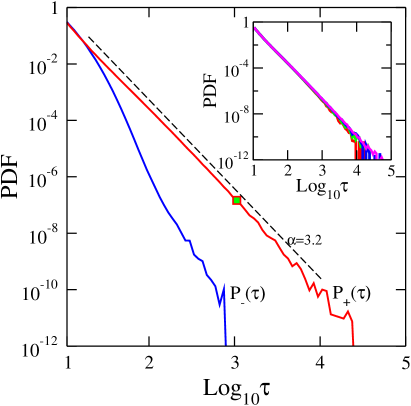
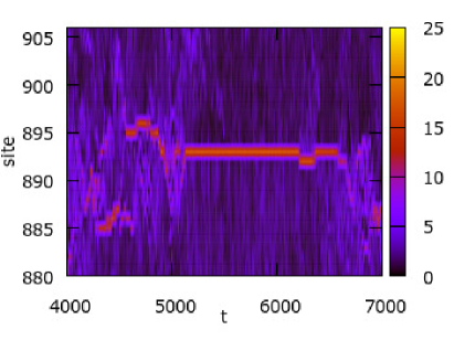
Figure 2: (Color online) (a) $P_{\pm}(\tau)$ for $x=2,\leavevmode\nobreak\ y=4$ (on the $\beta=0$ line) for $N=2^{10}$. The upper red curve indicates $P_{+}(\tau)$ and bottom blue curve for $P_{-}(\tau)$. The dashed line is an algebraic decay $\tau^{-\alpha}$ with $\alpha=3.2$. Inset: $P_{+}(\tau)$ for different system sizes $N=512,1024,2048,4096$). (b) Time evolution of density, $|\psi_{n}|^{2}$ in correspondence of one of the excursion time $\tau$ marked with the green colored square in Fig. 2(a). Here $g=1$.

In Fig.2(a) we show $P_{\pm}(\tau)$ for a density pair $x=2,\leavevmode\nobreak\ y=4$ on the $\beta=0$ line $y_{nG}(x)$. We observe that $P_{+}(\tau)$ (upper red curve) has a clear algebraic tail, while $P_{-}(\tau)$ (lower blue curve) decays much faster, and in a more complex manner. In the following we will present results for the exponent $\alpha$ for $P_{+}(\tau)$ only, which reads $\alpha=3.2\pm 0.1$. By our definition, the dynamics is ergodic, despite being on the border line to the nonGibbs phase. We plot in the inset of Fig.2(a) the function $P_{+}(\tau)$ obtained for different volumes $N=512,1024,2048,4096$ and conclude that we can exclude the impact of finite size effects. In Fig.2(b), we show the time evolution of the norm density of one of the excursions which contribute to the algebraic tail (marked with the green square in Fig.2(a)). We observe the generation of a long lasting discrete breather like excitation out of ergodic fluctuations, which persists for a large time $10^{3}$ and finally decays again into the thermalized surrounding. We positively tested this conclusion for many other tail excursions.

In Fig.3 we present results for the exponent $\alpha$ along the two characteristic lines $y_{h}(x)$ and $y_{nG}(x)$. The function $\alpha_{nG}(x)$ along the $\beta=0$ line $y_{nG}(x)=x^{2}$ (which separates Gibbs and nonGibbs phases) monotonously decreases with increasing $x$. Its value is clearly $\alpha>2$ in the whole assessed range $0<x<6$. We may anticipate that weak nonergodicity ($\alpha=2$) happens around $x\sim 20-30$ in that line. The function $\alpha_{h}(x)$ along the limiting line for homogeneous states $y_{h}(x)=2x+x^{2}/2$ is monotonously decreasing with decreasing $x$. While increasing density $x$ enhances ergodicity on that line, we observe a transition to weak nonergodicity $\alpha_{h}<2$ for $x<2$. Let us remind that in the weakly nonergodic regime every observable becomes trajectory dependent for any finite averaging time. This dependence translates into large uncertainties in their measurement, which herewith results in the large error bars in Fig.3 for $\alpha\sim 2$ (details of the estimate of the exponent $\alpha$ are given in the supplemental material Sup ). The transition to weak nonergodicity happens well in the nonGibbs phase. Therefore we conclude that parts of the nonGibbs phase allow for ergodic dynamics. This in turn implies that a new nonGibbs distribution function should exist. We also mapped the density space points which correspond to $\alpha=2$ into a line $y_{NE}(x)$ in Fig.1. This line is clearly located inside the nonGibbs phase, albeit close to its boundary.

The Lyapunov exponent function $\Lambda_{nG}(x)$ along the $\beta=0$ line $y_{nG}(x)$, and the function $\Lambda_{h}(x)$ along the $y_{h}(x)$ line, are plotted in Fig.3 and show no anomalies, neither in the ergodic, nor in the weakly nonergodic, neither in the Gibbs, nor in the nonGibbs phases. Therefore, we conclude that weakly nonergodic dynamics is triggered by local fluctuations (discrete breather like excitations) which leave a part of the system well thermalized in between them. The Lyapunov exponent is sensitive to the chaotic dynamics in these thermalized puddles, but is not sensitive to the presence of weakly nonergodic boundaries between the puddles.

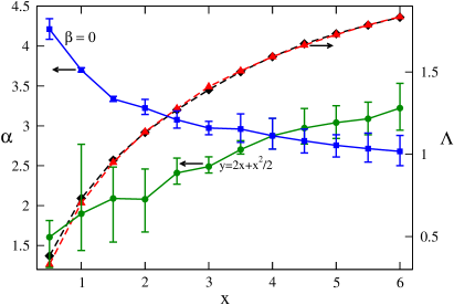
Figure 3: (Color online) The exponent $\alpha$ of the power-law tail for the norm density $x$ calculated along the two lines $y_{nG}=x^{2}$ (blue solid line) and $y_{h}=2x+\frac{x^{2}}{2}$ (green solid line). The dashed black and red lines represent the mLCE ($\Lambda(x)$) along the lines $y_{nG}$ and $y_{h}$, respectively.

Let us discuss our observations. The Gross–Pitaevskii lattice model is one of the remarkable cases where the large density limit yields an integrable system of disconnected anharmonic oscillators. The network of nonintegrable perturbations which couple the actions off that limit is given by the hopping part of the GP model, and is short ranged. As a consequence, the microcanonical dynamics becomes weakly nonergodic at large but finite densities for a macroscopic system, which is still at a finite distance from some integrable limit. We quantify these observations by computing distributions of excursion times off equilibrium Poincare manifolds, and measuring the exponents in their tails. Long excursion times are related to the generation of hot spots, or discrete breather like excitations. Our method is therefore able to quantitatively assess discrete breather lifetimes at equilibrium. Note that weakly nonergodic dynamics is going well along with nonzero Lyapunov exponents. This happens because a part of the system condenses into discrete breather like regions, or spots of regular dynamics, while regions between these spots still evolve in a chaotic fashion.

It is tempting to relate these observations to the existence of a nonGibbs phase in the microcanonical GP lattice dynamics. Note that this nonGibbs phase existence follows from the existence of a second conserved quantity (the norm aka particle number) and is a result of a purely statistical analysis. We find that a part of the nonGibbs phase is ergodic. Therefore we conclude that a yet unknown new grand canonical distribution function might exist which describes the equilibrium and ergodic dynamics there. Nevertheless, the explicit form of this distribution function is not known. At the same time, we expect that weakly nonergodic dynamics due to large densities will also take place in the Gibbs part of the microcanonical control parameter space.

The microcanonical thermodynamical description as well as the existence of negative temperature for Hamiltonian systems with bounded spectrum have been questioned by Duenkel et. al. in Dunkel and Hilbert (2014). Their argument says that, in order to describe the thermodynamics of such systems, the Gibbs entropy has to be employed, which implies the non-existence of negative temperature. In our case, we followed the microcanonical ergodic dynamics defined with the Boltzmann temperature and is proven to be valid in the defined Gibbs phase. Moreover, it has been recently shown that the Boltzmann entropy (which admits negative temperatures) provides the correct description of the microcanonical thermodynamics of systems like the GP Buonsante et al. (2016, 2017) (further discussions can be found in Rumpf (2004, 2008, 2009); Iubini et al. (2012, 2013)).

To conclude, we applied a novel method of statistical analysis of excursion times off equilibrium Poincare manifolds to the transition from ergodic to nonergodic dynamics in the Gross–Pitaevskii lattice model. Our results are in analogy with the weak nonergodicity phenomena studied in glass systems Bouchaud (1992), continuous-time random walks Bel and Barkai (2005, 2006); Rebenshtok and Barkai (2007), as well as in other many-body systems Danieli et al. (2017). We expect them to be applicable also to larger spatial dimensions, and to other lattice models with similar integrable limits. We also speculate that spatial disorder, which induces Anderson localization, at small densities will again lead to weakly nonergodic dynamics at (then small but) finite densities.

I Acknowledgements

The authors acknowledge financial support from IBS (Project Code No. IBS-R024-D1). We thank I. Vakulchyk, A. Andreanov and C. H. Skokos for helpful discussions.

Supplemental Material for: ’Weakly nonergodic dynamics in the Gross–Pitaevskii lattice’

II LCE Calculation

The variational equation

$$i\dot{\chi}_{m}=-(\chi_{m+1}+\chi_{m-1})+g(2|\psi_{m}|^{2}\chi_{m}+\psi_{m}^{2}\chi_{m}^{\ast}),$$ (6)

is solved by using symplectic $SBAB_{2}$ integrator scheme. The Hamiltonian,

$$\mathcal{H}=\sum_{m}\big{[}-(\chi_{m}^{\ast}\chi_{m+1}+\chi_{m}\chi_{m+1}^{\ast})+\frac{g}{2}(4|\psi_{m}|^{2}|\chi_{m}|^{2}+\psi_{m}^{2}\chi_{m}^{\ast 2})\big{]}$$ (7)

corresponds to Eq. (6) is split as

$$A=\sum_{m}\big{[}-(\chi_{m}^{\ast}\chi_{m+1}+\chi_{m}\chi_{m+1}^{\ast})\big{]},$$ (8)

$$B=\frac{g}{2}\sum_{m}\big{[}(4|\psi_{m}|^{2}|\chi_{m}|^{2}+\psi_{m}^{2}\chi_{m}^{\ast 2})\big{]}.$$ (9)

B can be written as $B=P+Q$, where

$$\small P=2g\sum_{m}|\psi_{m}|^{2}|\chi_{m}|^{2},\leavevmode\nobreak\ \leavevmode\nobreak\ Q=\frac{g}{2}\sum_{m}\psi_{m}^{2}\chi_{m}^{\ast 2}$$ (10)

II.0.1 Action of the operator $e^{\tau L_{A}}$ on $\chi_{m}$

Fast Fourier transform (FFT) is used for Hamiltonian $A$.

$$\chi_{q}=\sum_{l=1}^{N}\chi_{l}e^{2\pi i(q-1)(l-1)/N},$$ (11)

$$\chi_{q}^{{}^{\prime}}=\chi_{q}e^{2i\cos(2\pi(q-1)/N)\tau},$$ (12)

$$\chi_{m}^{{}^{\prime}}=\frac{1}{N}\sum_{q=1}^{N}\chi_{q}^{{}^{\prime}}e^{-2\pi i(m-1)(q-1)/N},$$ (13)

where $\chi_{m}^{{}^{\prime}}$ is $\chi_{m}$ at $t+\tau$.

II.0.2 Action of the operator $e^{\tau L_{P}}$ on $\chi_{m}$

It can be solved exactly as

$$\chi_{m}^{{}^{\prime}}=\chi_{m}e^{-2gi|\psi_{m}|^{2}\tau}$$ (14)

II.0.3 Action of the operator $e^{\tau L_{Q}}$ on $\chi_{m}$

$$\chi_{m}^{{}^{\prime}}=(\chi_{am}+i\chi_{bm}),$$ (15)

where

$$\chi_{am}=c_{1}\cosh(A\tau)+\frac{1}{A}\sinh(A\tau)\big{[}bc_{1}-ac_{2}\big{]},$$ (16)

$$\chi_{bm}=c_{2}\cosh(A\tau)-\frac{1}{A}\sinh(A\tau)\big{[}bc_{2}+ac_{1}\big{]},$$ (17)

where $A=\sqrt{a^{2}+b^{2}}$, $a=Re(g\psi_{m}^{2})$, $b=Im(g\psi_{m}^{2})$, $c_{1}=Re(\chi_{m})$ and $c_{2}=Im(\chi_{m})$. Equations are integrated by using the $SBAB_{2}$ scheme given in Bodyfelt et al. (2011).

Table 1: Calculation of $\Lambda(t)$

x	$y=x^{2}$	$\Lambda$	$y=2x+\frac{x^{2}}{2}$	$\Lambda$
0.5	0.25	0.3823	1.125	0.3308
1.0	1.0	0.7323	2.5	0.7049
1.5	2.25	0.9642	4.125	0.9505
2.0	4.0	1.1328	6	1.1369
2.5	6.25	1.2701	8.125	1.2774
3.0	9.0	1.3922	10.5	1.4107
3.5	12.25	1.5017	13.125	1.5066
4.0	16.0	1.5932	16	1.5932

In Fig. (4), the evolution of mLCE is depicted for norm density $x=2$. The energy density varies from Gibbs regime to nonGibbs regime. The mLCE saturates after $t=10^{7}$ and we calculate it by taking the average of mLCE for the range $t=10^{7}-10^{8}$. The positive value of mLCE says that the system is chaotic in both Gibbs regime and nonGibbs regime. The comparison of mLCE at Gibbs regime, at $y=4$ and $y=3$, reveals that the chaos in the system is directly proportional to the energy density and such dependency is observed for the problem of quartic Klein-Gordon chain of coupled anharmonic oscillators Skokos et al. (2013). Tab. 1 shows the mLCE for the various values of norm density. We could see that chaos is proportional to the norm density too. The main result is that mLCE in the nonergodic regime approaches its value at the phase transition line. It elucidates that change from the ergodic to nonergodic transition is extremely slow.

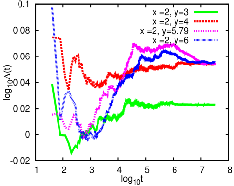
Figure 4: (Color online) Time evolution of the maximal Lyapunov exponent for the fixed norm density $x=2$. The different y values represent the Gibbs regime ($y=3$), the phase transition line ($y=x^{2}$), the ergodic to nonergodic transition line ($y=5.79$) and the nonGibbs regime.

Fitting $\alpha$ in the tails of $P_{+}(\tau)$

The PDF $P_{+}(\tau)$ is obtained using bins equispaced on a logarithmic scale. We estimate the exponent $\alpha$ by smoothening the curve $P_{+}(\tau)$ and using the Hodrick-Prescott filter method Hodrick and Prescott (1997). The extrapolation method has been used on intervals in the tail of the PDF, by fixing the upper interval bound $\tau^{M}$ and varying the lower bound $\tau^{m}$. The upper bound $\tau^{M}$ is defined by the first bin which counts zero events. In Fig.5 we show two PDFs which correspond to two cases on the green line of Fig.3 of the main text, for $(x,y)=(3,10)$ (Fig.5(a)) and $(x,y)=(1.5,4.125)$ (Fig.5(b)). In the insets, we show the exponent $\alpha$ measured as a function of the lower bound $\tau^{m}$. The horizontal line represents the final measured value, while the arrows represent the largest distances from the final value. These distances then become the error bars in Fig.3 of the main text. In Fig.5(a), the system is ergodic ($\alpha=2.5$) and the PDF shows a power-law trend. In Fig.5(b), the PDF shows a more complex trend. The curve is actually nowhere really close to a power law, and could decay even slower than any algebraic decay. The above defined error becomes of the order of the mean, which in fact means that the measured exponent is not very meaningful.

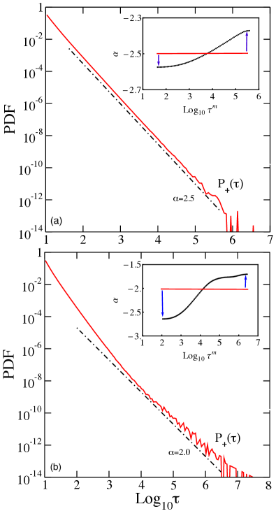
Figure 5: (Color online) PDF $P_{+}(\tau)$ obtained for $(x,y)=(3,10)$ and $(x,y)=(1.5,4.125)$. Insets: exponent $\alpha$ versus the lower bound $\tau^{m}$.

References

- Fermi et al. (1955) E. Fermi, J. Pasta, and S. Ulam, “Los alamos scientific laboratory report,” LA-1940 (1955).
- Ford (1992) J. Ford, “The fermi-pasta-ulam problem: Paradox turns discovery,” Phys. Rep. 213, 271 (1992).
- Rasmussen et al. (2000) K. O. Rasmussen, T. Cretegny, P. G. Kevrekidis, and N. Grønbech-Jensen, “Statistical mechanics of a discrete nonlinear system,” Phys. Rev. Lett. 84, 3740 (2000).
- Rumpf (2004) B. Rumpf, “Simple statistical explanation for the localization of energy in nonlinear lattices with two conserved quantities,” Phys. Rev. E 69, 016618 (2004).
- Rumpf (2008) B. Rumpf, “Transition behavior of the discrete nonlinear schrödinger equation,” Phys. Rev. E 77, 036606 (2008).
- Rumpf (2009) B. Rumpf, “Stable and metastable states and the formation and destruction of breathers in the discrete nonlinear schrödinger equation,” Physica D 238, 2067 (2009).
- Iubini et al. (2012) S. Iubini, S. Lepri, and A. Politi, “Nonequilibrium discrete nonlinear schrödinger equation,” Phys. Rev. E 86, 011108 (2012).
- Iubini et al. (2013) S. Iubini, R. Franzosi, R. Livi, G.-L. Oppo, and A. Politi, “Discrete breathers and negative-temperature states,” New J. Phys. 15, 023032 (2013).
- Livi et al. (2006) R. Livi, R. Franzosi, and G.-L. Oppo, “Self-localization of bose-einstein condensates in optical lattices via boundary dissipation,” Phys. Rev. Lett. 97, 060401 (2006).
- Hennig and Fleischmann (2013) H. Hennig and R. Fleischmann, “Nature of self-localization of bose-einstein condensates in optical lattices,” Phys. Rev. A 87, 033605 (2013).
- Kruse and Fleischmann (2017) J. Kruse and R. Fleischmann, “Self-localization of bose-einstein condensates in optical lattices,” J. Phys. B: At. Mol. Opt. Phys. 50, 055002 (2017).
- Ivanchenko et al. (2004) M. V. Ivanchenko, O. Kanakov, V. Shalfeev, and S. Flach, “Discrete breathers in transient processes and thermal equilibrium,” Physica D 198, 120 (2004).
- Pino et al. (2016) M. Pino, L. B. Ioffe, and B. L. Altshuler, “Nonergodic metallic and insulating phases of josephson junction chains,” PNAS 113, 536 (2016).
- Bouchaud (1992) J.-P. Bouchaud, “Weak ergodicity breaking and aging in disordered systems,” Journal de Physique I 2, 1705 (1992).
- Bel and Barkai (2005) G. Bel and E. Barkai, “Weak ergodicity breaking in the continuous-time random walk,” Physical Review Letters 94, 240602 (2005).
- Bel and Barkai (2006) G. Bel and E. Barkai, “Random walk to a nonergodic equilibrium concept,” Physical Review E 73, 016125 (2006).
- Rebenshtok and Barkai (2007) A. Rebenshtok and E. Barkai, “Distribution of time-averaged observables for weak ergodicity breaking,” Physical review letters 99, 210601 (2007).
- Lutz (2004) E. Lutz, “Power-law tail distributions and nonergodicity,” Physical review letters 93, 190602 (2004).
- Danieli et al. (2017) C. Danieli, D. K. Campbell, and S. Flach, “Intermittent many-body dynamics at equilibrium,” Phys. Rev. E 95, 060202 (2017).
- Flach and Willis (1998) S. Flach and C. Willis, “Discrete breathers,” Phys. Rep. 295, 181 (1998).
- Campbell et al. (2004) D. K. Campbell, S. Flach, and Y. S. Kivshar, “Localizing energy through nonlinearity and discreteness,” Physics Today 57, 43 (2004).
- Flach and Gorbach (2008) S. Flach and A. V. Gorbach, “Discrete breathers - advances in theory and applications,” Phys. Rep. 467, 1 (2008).
- Franzosi et al. (2011) R. Franzosi, R. Livi, G.-L. Oppo, and A. Politi, “Discrete breathers in bose-einstein condensates,” Nonlinearity 24, R89 (2011).
- MacKay and Aubry (1994) R. MacKay and S. Aubry, “Proof of existence of breathers for time-reversible or hamiltonian networks of weakly coupled oscillators,” Nonlinearity 7, 1623 (1994).
- Skokos et al. (2009) C. Skokos, D. O. Krimer, S. Komineas, and S. Flach, “Delocalization of wave packets in disordered nonlinear chains,” Phys. Rev. E 79, 056211 (2009).
- Skokos et al. (2016) C. H. Skokos, G. A. Gottwald, and J. Laskar, Chaos Detection and Predictability, Lecture Notes in Physics, Vol. 915 (Springer, Berlin, 2016).
- Johansson et al. (2010) M. Johansson, G. Kopidakis, and S. Aubry, “Kam tori in 1d random discrete nonlinear schrödinger model?” EPL (Europhysics Letters) 91, 50001 (2010).
- (28) See Supplemental Material at [URL will be inserted by publisher] for additional information .
- Dunkel and Hilbert (2014) J. Dunkel and S. Hilbert, “Consistent thermostatistics forbids negative absolute temperatures,” Nature Physics 10, 67 (2014).
- Buonsante et al. (2016) P. Buonsante, R. Franzosi, and A. Smerzi, “On the dispute between boltzmann and gibbs entropy,” Annals of Physics 375, 414 (2016).
- Buonsante et al. (2017) P. Buonsante, R. Franzosi, and A. Smerzi, “Phase transitions at high energy vindicate negative microcanonical temperature,” Phys. Rev. E 95, 052135 (2017).
- Bodyfelt et al. (2011) J. D. Bodyfelt, T. V. Laptyeva, C. Skokos, D. O. Krimer, and S. Flach, “Nonlinear waves in disordered chains: Probing the limits of chaos and spreading,” Phys. Rev. E 84, 016205 (2011).
- Skokos et al. (2013) C. Skokos, I. Gkolias, and S. Flach, “Nonequilibrium chaos of disordered nonlinear waves,” Phys. Rev. Lett. 111, 064101 (2013).
- Hodrick and Prescott (1997) R. J. Hodrick and E. C. Prescott, “Postwar us business cycles: an empirical investigation,” Journal of Money, credit, and Banking , 1 (1997).