Angular Schmidt spectrum of entangled photons: derivation of an exact formula and experimental characterization for non-collinear phase matching

Abstract

We derive an exact computationally-efficient formula for the angular Schmidt spectrum of orbital angular momentum (OAM)-entangled states produced by parametric down-conversion (PDC). Our formula yields the true spectrum and does not suffer from convergence issues arising due to infinite summations, as has been the case with previously derived formulas. We use this formula to experimentally characterize the angular Schmidt spectrum of entangled photons produced by PDC with non-collinear phase matching. We report measurements of very broad angular Schmidt spectra, corresponding to the angular Schmidt numbers up to 229. Our studies can have important implications for OAM-based quantum information applications.

I Introduction

High-dimensional quantum information protocols offer many distinct advantages in terms of security karimipour2002pra ; cerf2002prl ; nikolopoulos2006pra , supersensitive measurements jha2011pra2 , violation of bipartite Bell’s inquality collins2002prl ; leach2009optexp ; vetesi2010prl , enhancement of entanglement via concentration vaziri2003prl , and implementation of quantum coin-tossing protocol terriza2005prl . After it was shown that the orbital angular momentum (OAM) of a photon provides a high-dimensional basis allen1992pra ; barnett1990pra ; yao2006opex , the OAM-entangled states of signal and idler photons produced by parametric down-conversion (PDC) have become a natural choice for high-dimensional quantum information applications. To this end, there have been intense research efforts, both theoretically law2004prl ; torres2003pra ; miatto2011pra ; yao2011njp ; jha2011pra ; miatto2012epjd ; zhang2014pra and experimentally mair2001nature ; pors2008prl ; jha2010prl ; peeters2007pra ; pires2010prl ; giovannini2012njp ; kulkarni2017natcomm , for the precise characterization of high-dimensional OAM-entangled states produced by PDC. Although a general OAM-entangled state requires the full state tomography for its characterization, the experimentally relevant case of OAM-entangled states produced using a Gaussian pump beam can be characterized by measuring just the angular Schmidt spectrum law2004prl ; torres2003pra ; pires2010prl , which is defined as the probability $S_{l}$ of signal and idler photons getting detected with OAMs $l\hbar$ and $-l\hbar$, respectively.

The characterization of the angular Schmidt spectrum has been a very challenging problem. On the experimental front, several techniques have been developed for measuring the angular Schmidt spectrum. The first set of techniques is based on using fiber-based projective measurements mair2001nature ; jha2010prl ; pors2008prl ; peeters2007pra ; giovannini2012njp . However, these techniques are very inefficient because the required number of measurements scales with the size of the input spectrum. Furthermore, these techniques measure only the projected spectrum instead of the true spectrum qassim2014josab . The second set of techniques is based on inferring the spectrum by measuring the angular coherence function pires2010prl ; jha2011pra . Although these techniques do measure the true spectrum, they either require a series of coincidence measurements and have strict interferometric stability requirements pires2010prl or suffer from too much loss jha2011pra . More recently, an interferometric technique has been demonstrated that can measure the true angular Schmidt spectrum in a very efficient single-shot manner kulkarni2017natcomm . On the theoretical front, Torres et al. have derived a formula for calculating the spectrum for collinear phase matching torres2003pra . However, this formula involves a four-dimensional integration followed by two infinite summations over the radial indices. Although the summations have been shown to converge for certain set of experimental parameters, the convergence is not explicitly proved for an arbitrary set of parameters. Moreover, it is extremely inefficient to first calculate the contributions due to sufficiently large number of radial modes and then sum them over. Subsequent studies have analytically performed the four-dimensional integration for certain collinear phase-matching conditions miatto2011pra ; yao2011njp , but they still suffer from the same set of issues due to infinite summations. There has been a recent investigatoin by Zhang and Roux for the non-collinear phase matching condition zhang2014pra , however, the angular Schmidt spectrum calculated in this study is only for a given pair of radial modes of the signal and idler photons, and therefore is not applicable to a generic experimental situation.

Thus, although the past efforts have been able to greatly overcome the experimental challenges in measuring the true Schmidt spectrum, the theoretical challenge of deriving an exact formula has so far remained unresolved. In this article, we derive an exact formula for calculating the true angular Schmidt spectrum that does not suffer from the above mentioned issues since the infinite summations over radial modes are performed analytically. Moreover, our formula is valid for both collinear and non-collinear phase matching conditions. Using this formula, we report experimental characterizations of the angular Schmidt spectrum with various non-collinear phase-matching conditions.

II Theory

II.1 Derivation of the general formula

The state $|\psi_{2}\rangle$ of the down-converted photons is written in the transverse-momentum basis as hong1985pra :

$$|\psi_{2}\rangle=\iint_{-\infty}^{\infty}\Phi({\bm{q_{s}},{\bm{q}_{i}}})|{\bm{q}_{s}}\rangle_{s}|{\bm{q}_{i}}\rangle_{i}d\bm{q}_{s}d\bm{q}_{i},$$ (1)

where, $s$, and $i$ stand for signal, and idler, respectively, and where $|{\bm{q}_{s}}\rangle$ and $|{\bm{q}_{i}}\rangle$ denote the states of the signal and idler photons with transverse momenta $\bm{q}_{s}$ and $\bm{q}_{i}$, respectively. $\Phi({\bm{q_{s}},{\bm{q}_{i}}})$ is the wavefunction of the down-converted photons in the transverse-momentum basis; it depends on the detailed properties of the pump field, the nonlinear crystal, and the phase matching condition hong1985pra ; torres2003pra ; walborn2010physrep . The state $|\psi_{2}\rangle$ can also be represented in the Laguerre-Gaussian (LG) basis torres2003pra ; miatto2011pra ; yao2011njp ; jha2011pra as:

$$|\psi_{2}\rangle=\sum_{l_{s}}\sum_{l_{i}}\sum_{p_{s}}\sum_{p_{i}}C^{l_{s},p_{s}}_{l_{i},p_{i}}|l_{s},p_{s}\rangle_{s}|l_{i},p_{i}\rangle_{i}.$$ (2)

Here $|l_{s},p_{s}\rangle_{s}$ represents the state of the signal photon in the Laguerre-Gaussian (LG) basis defined by the OAM-mode index $l_{s}$ and the radial index $p_{s}$, etc. Using Eqs. (1) and (2), the complex coefficients $C^{l_{s},p_{s}}_{l_{i},p_{i}}$ can be written as,

$$\!\!C^{l_{s},p_{s}}_{l_{i},p_{i}}=\!\!\iint\!\!\Phi({\bm{q}_{s}},{\bm{q}_{i}})LG^{*l_{s}}_{p_{s}}({\bm{q}_{s}})LG^{*l_{i}}_{p_{i}}({\bm{q}_{i}})d{\bm{q}_{s}}d{\bm{q}_{i}}.$$ (3)

Here $LG^{l_{s}}_{p_{s}}({\bm{q}_{s}})=\langle{\bm{q}_{s}}|l_{s},p_{s}\rangle$ is the momentum-basis representation of state $|l_{s},p_{s}\rangle_{s}$ torres2003pra ; miatto2011pra . Transforming to the cylindrical coordinates, we write $C^{l_{s},p_{s}}_{l_{i},p_{i}}$ as,

$$C^{l_{s},p_{s}}_{l_{i},p_{i}}=\iint_{0}^{\infty}\iint_{-\pi}^{\pi}\Phi(\rho_{s},\rho_{i},\phi_{s},\phi_{i})\\ \times LG^{*l_{s}}_{p_{s}}(\rho_{s},\phi_{s})LG^{*l_{i}}_{p_{i}}(\rho_{i},\phi_{i})\rho_{s}\rho_{i}d\rho_{s}d\rho_{i}d\phi_{s}d\phi_{i},$$ (4)

where ${\bm{q}_{s}}\equiv(q_{sx},q_{sy})=(\rho_{s}\cos\phi_{s},\rho_{s}\sin\phi_{s})$, ${\bm{q}_{i}}\equiv(q_{ix},q_{iy})=(\rho_{i}\cos\phi_{i},\rho_{i}\sin\phi_{i})$, $d{\bm{q}_{s}}=\rho_{s}d\rho_{s}d\phi_{s}$, and $d{\bm{q}_{i}}=\rho_{i}d\rho_{i}d\phi_{i}$. The probability $P^{l_{s}}_{l_{i}}$, that the signal and idler photons are detected with OAMs $l_{s}\hbar$ and $l_{i}\hbar$, respectively, is calculated by summing over radial indices:

$$P^{l_{s}}_{l_{i}}=\sum_{p_{s}=0}^{\infty}\sum_{p_{i}=0}^{\infty}|C^{l_{s},p_{s}}_{l_{i},p_{i}}|^{2}.$$ (5)

Eqs. (4) and (5) were used in Refs. torres2003pra ; miatto2011pra ; yao2011njp for calculating the specta of OAM-entangled states. We note that in order to calculate the angular Schmidt spectrum using the above formula one needs to first choose a beam waist for the signal and idler LG bases in Eqs. (4)and then perform the summations in Eq. (5) over a sufficiently large number of modes. As a result, even for certain collinear phase-matching conditions, in which the four-dimensional integral can be analytically performed miatto2011pra ; yao2011njp , the above formula suffers from convergence issues.

We next present the derivation of a formula for the angular Schmidt spectrum that neither requires a beam waist to be chosen nor involves infinite summations and is applicable to both collinear and non-collinear phase matching conditions. To this end, we first rewrite Eq. (5) using the relation $LG^{l_{s}}_{p_{s}}(\rho_{s},\phi_{s})=LG_{p_{s}}^{l_{s}}(\rho_{s})e^{il_{s}\phi_{s}}$, etc., as

$$P^{l_{s}}_{l_{i}} =\iiiint_{0}^{\infty}\iiiint_{-\pi}^{\pi}\Phi(\rho_{s},\rho_{i},\phi_{s},\phi_{i})\Phi^{*}(\rho^{\prime}_{s},\rho^{\prime}_{i},\phi^{\prime}_{s},\phi^{\prime}_{i})$$

$$\times\sum_{p_{s}=0}^{\infty}LG^{*l_{s}}_{p_{s}}(\rho_{s})LG^{l_{s}}_{p_{s}}(\rho^{\prime}_{s})\sum_{p_{i}=0}^{\infty}LG^{*l_{i}}_{p_{i}}(\rho_{i})LG^{l_{i}}_{p_{i}}(\rho^{\prime}_{i})$$

$$\times e^{+i(l_{s}\phi_{s}+l_{i}\phi_{i})}e^{-i(l_{s}\phi^{\prime}_{s}+l_{i}\phi^{\prime}_{i})}$$

$$\times\rho_{s}\rho_{i}\rho^{\prime}_{s}\rho^{\prime}_{i}d\rho_{s}d\rho_{i}d\rho^{\prime}_{s}d\rho^{\prime}_{i}d\phi_{s}d\phi_{i}d\phi^{\prime}_{s}d\phi^{\prime}_{i}.$$ (6)

We then use the identity $\sum_{p=0}^{\infty}LG^{p}_{l}(\rho)LG^{*^{p}}_{l}(\rho^{\prime})=(1/\pi)\delta(\rho^{2}-\rho^{\prime 2})$ over indices $p_{s}$ and $p_{i}$ and obtain

$$P^{l_{s}}_{l_{i}} =\iiiint_{0}^{\infty}\iiiint_{-\pi}^{\pi}\Phi(\rho_{s},\rho_{i},\phi_{s},\phi_{i})\Phi^{*}(\rho^{\prime}_{s},\rho^{\prime}_{i},\phi^{\prime}_{s},\phi^{\prime}_{i})$$

$$\times\frac{1}{\pi^{2}}\delta(\rho_{s}^{2}-\rho^{\prime 2}_{s})\delta(\rho_{i}^{2}-\rho^{\prime 2}_{i})e^{+i(l_{s}\phi_{s}+l_{i}\phi_{i})}e^{-i(l_{s}\phi^{\prime}_{s}+l_{i}\phi^{\prime}_{i})}$$

$$\times\rho_{s}\rho_{i}\rho^{\prime}_{s}\rho^{\prime}_{i}d\rho_{s}d\rho_{i}d\rho^{\prime}_{s}d\rho^{\prime}_{i}d\phi_{s}d\phi_{i}d\phi^{\prime}_{s}d\phi^{\prime}_{i}.$$ (7)

After evaluating the delta function integrals and rearranging the remaining terms, we obtain

$$P^{l_{s}}_{l_{i}}=\frac{1}{4\pi^{2}}\iint_{0}^{\infty} {\Big{|}}\iint_{-\pi}^{\pi}\Phi(\rho_{s},\rho_{i},\phi_{s},\phi_{i})$$

$$\times e^{i(l_{s}\phi_{s}+l_{i}\phi_{i})}d\phi_{s}d\phi_{i}{\Big{|}}^{2}\rho_{s}\rho_{i}d\rho_{s}d\rho_{i}.$$ (8)

Now, we take up the most common experimental situation in which the OAM remains conserved during down-conversion, that is, $l_{p}=l_{s}+l_{i}$, which for a Gaussian pump beam with $l_{p}=0$ implies that $l_{s}=-l_{i}=l$ mair2001nature . In these situations, the down-converted two-photon state $|\psi_{2}\rangle$ of Eq. (2) takes the following form law2004prl ; torres2003pra ; miatto2011pra ; yao2011njp ; jha2011pra : $|\psi_{2}\rangle=\sum_{l}\sum_{p_{s}}\sum_{p_{i}}C^{l,p_{s}}_{-l,p_{i}}|l,p_{s}\rangle_{s}|-l,p_{i}\rangle_{i}$, which, when written with only the OAM-mode index as the label for the state, takes the Schmidt decomposed form: $|\psi_{2}\rangle=\sum_{l=-\infty}^{\infty}\sqrt{S_{l}}|l\rangle_{s}|-l\rangle_{i}$. The corresponding angular Schmidt spectrum $S_{l}=P_{l}^{-l}$ is the probability that the signal and idler photons have OAMs $l\hbar$ and $-l\hbar$, respectively, and using Eq. (8) it can be written as

$$S_{l}=\frac{1}{4\pi^{2}}\iint_{0}^{\infty} {\Big{|}}\iint_{-\pi}^{\pi}\Phi(\rho_{s},\rho_{i},\phi_{s},\phi_{i})$$

$$\times e^{il(\phi_{s}-\phi_{i})}d\phi_{s}d\phi_{i}{\Big{|}}^{2}\rho_{s}\rho_{i}d\rho_{s}d\rho_{i}.$$ (9)

Equations (8) and (9) are the main theoretical results of this article. While Eq. (8) provides a formula for calculating the probability $P^{l_{s}}_{l_{i}}$ that the signal and idler photons are detected with OAMs $l_{s}\hbar$ and $l_{i}\hbar$, respectively, Eq. (9) calculates the angular Schmidt spectrum. In contrast to the previously obtained formulas torres2003pra ; miatto2011pra ; yao2011njp ; zhang2014pra , Eqs. (8) and (9) neither require a beam waist to be chosen nor involve infinite summations. As a result, these formulas can provide improvement of several orders of magnitude in the spectrum computation time. Moreover, unlike the non-collinear phase-matching results in Ref. zhang2014pra , which is applicable only for a given pair of radial modes of the signal and idler photons, these formulas are applicable to a generic set of non-collinear phase matching conditions and geometries. We note that although the above formulas do not have any convergence issue arising due to infinite summations, the definite integrals might have convergence issues for some arbitrary functional form of $\Phi(\rho_{s},\rho_{i},\phi_{s},\phi_{i})$. However, we do not expect such convergence issues for the commonly encountered forms of $\Phi(\rho_{s},\rho_{i},\phi_{s},\phi_{i})$ for collinear and non-collinear phase matching conditions. In order to illustrate this and to describe our experiments presented later, we next derive the momentum-space wavefunction $\Phi(\rho_{s},\rho_{i},\phi_{s},\phi_{i})$ for the case of collinear type-I down-conversion and calculate the angular Schmidt spectrum.

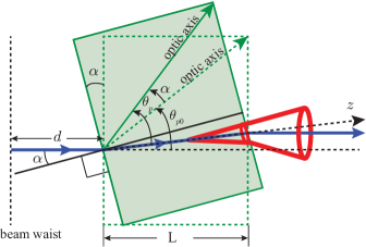
Figure 1: (color online) Schematic of phase matching in PDC.

II.2 The special case of a Gaussian pump beam

Let us consider the situation shown in Fig. 1. A Gaussian pump beam undergoes Type-I PDC inside a nonlinear crystal of thickness $L$. We take the pump photon to be extra-ordinary polarized and the signal and idler photons to be ordinary polarized. The beam waist of the pump field is located at a distance $d$ behind the front surface of the crystal. The crystal is rotated by an angle $\alpha$ with respect to the incident direction of the pump beam, and the $z$-axis is defined to be the direction of the refracted pump beam inside the crystal. The angles that the optic axes of the unrotated and rotated crystals make with the pump beam inside the crystal are denoted by $\theta_{p0}$ and $\theta_{p}$, respectively. Using Fig. 1, one can show that

$$\theta_{p}=\theta_{p0}+\sin^{-1}\left(\sin\alpha/\eta_{p}\right),$$ (10)

where $\eta_{p}$ is the refractive index of the extraordinary pump photons. By changing $\theta_{p}$, one can go from collinear to non-collinear down-conversion. The wavefunction $\Phi({\bm{q_{s}},{\bm{q}_{i}}})$ of the down-converted photons in the transverse-momentum basis at the exit surface inside the crystal is written as hong1985pra ; torres2003pra ; walborn2010physrep :

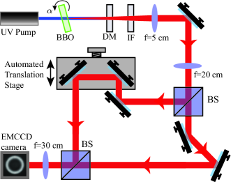
Figure 2: (color online) Experimental setup for measuring the angular Schmidt spectrum. BBO: $\beta$-Barium Borate crystal; DM: Dichroic mirror; IF: 10-nm wavelength-bandwidth interference filter; BS: beam splitter.

$$\Phi({\bm{q_{s}},{\bm{q}_{i}}})= AV({\bm{q}_{s}}+{\bm{q}_{i}})e^{ik_{pz}d}$$

$$\times\operatorname{sinc}\left(\frac{\Delta k_{z}L}{2}\right)\exp\left(i\frac{\Delta k_{z}L}{2}\right),$$ (11)

Here, again, $p$, $s$, and $i$ stand for pump, signal, and idler, respectively; $A$ is a constant and $\mathrm{sinc}(x)\equiv\sin x/x$. We have used ${\bm{k}_{j}}\equiv(k_{jx},k_{jy},k_{jz})\equiv(q_{jx},q_{jy},k_{jz})\equiv({\bm{q}_{j}},k_{jz})$, with $j=p,s,i$, and $\Delta k_{z}=k_{pz}-k_{sz}-k_{iz}$. The quasi-monochromaticity condition is assumed for each of the signal, idler and pump photons with their central wavelengths given by $\lambda_{s}$, $\lambda_{i}$, and $\lambda_{p}$, respectively. In addition, the transverse size of the crystal is taken to be much larger compared to the spot-size of the pump beam, ensuring ${\bm{q}_{p}}={\bm{q}_{s}}+{\bm{q}_{i}}$. The quantity $V({\bm{q}_{s}}+{\bm{q}_{i}})e^{ik_{pz}d}$ is the spectral amplitude of the pump field at $z=0$, wherein

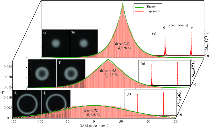
Figure 3: (color online) (a), (b) The measured output interferograms at $\delta=\delta_{c}$ and $\delta=\delta_{d}$, respectively, (c) the difference $\Delta{\bar{I}}(\phi)$ in the azimuthal intensities of the two inteferograms, (d) The normalized measured spectrum as computed using Eq. (15) and the normalized theoretical spectrum as calculated using Eq. (8), for $\alpha=0.33$ and $\theta_{p}=$28.64. (e), (f), (g), (h) are the corresponding plots for $\alpha=0.45$ and $\theta_{p}=$28.72. (i), (j), (k), (l) are the corresponding plots for $\alpha=0.73$ and $\theta_{p}=$28.89.

$$V({\bm{q}_{s}}+{\bm{q}_{i}})=\frac{w_{p}}{\sqrt{2\pi}}\exp\left(-\frac{|{\bm{q}_{s}}+{\bm{q}_{i}}|^{2}w_{p}^{2}}{4}\right)$$ (12)

is the spectral amplitude of the pump field at $z=0$ with $w_{p}$ being the width of the pump beam waist. We take the expressions for $k_{jz}$ from Ref. walborn2010physrep (a sign typo in the expression for $k_{pz}$ in Ref. walborn2010physrep has been corrected here):

$$k_{s_{z}}=\sqrt{\left(2\pi n_{so}/\lambda_{s}\right)^{2}-|{\bm{q}_{s}}|^{2}},$$

$$k_{i_{z}}=\sqrt{\left(2\pi n_{io}/\lambda_{i}\right)^{2}-|{\bm{q}_{i}}|^{2}},\ \ {\rm and}\$$

$$k_{p_{z}}=-\alpha_{p}q_{px}+\sqrt{\left(2\pi\eta_{p}/\lambda_{p}\right)^{2}-\beta_{p}^{2}q_{px}^{2}-\gamma_{p}^{2}q_{py}^{2}},$$ (13)

where

$$\eta_{p}=n_{pe}\gamma_{p},$$

$$\gamma_{p}=n_{po}/\sqrt{n_{po}^{2}\sin^{2}\theta_{p}+n_{pe}^{2}\cos^{2}\theta_{p}},$$

$$\alpha_{p}=\frac{(n_{po}^{2}-n_{pe}^{2})\sin\theta_{p}\cos\theta_{p}}{(n_{po}^{2}\sin^{2}\theta_{p}+n_{pe}^{2}\cos^{2}\theta_{p})},$$

$${\rm and}\ \ \beta_{p}=\frac{n_{po}n_{pe}}{(n_{po}^{2}\sin^{2}\theta_{p}+n_{pe}^{2}\cos^{2}\theta_{p})}.$$ (14)

Here $n_{so}$ denotes the ordinary refractive index of the signal photon at wavelength $\lambda_{s}$, etc. The angular Schmidt spectrum $S_{l}$ can be evaluated by substituting into Eq. (9) from Eqs. (11) through (14). We note that the formula in Eq. (9) represents angular Schmidt spectrum just inside the nonlinear crystal. Nevertheless, in situations in which $\alpha$ is of the order of only a few degrees, the angular Schmidt spectrum inside and outside the crystal can be taken to be the same.

Next, we use the experimental technique of Ref. kulkarni2017natcomm to characterize the angular Schmidt spectrum for non-collinear phase matching conditions and compare our experimental results with the theoretical predictions of Eq. (9). Figure 2 shows our experimental setup. Following Ref. kulkarni2017natcomm , we first define the measured OAM spectrum as

$$\bar{S_{l}}\equiv\int_{-\pi}^{\pi}\Delta\bar{I}_{\rm out}(\phi)e^{i2l\phi}d\phi,$$ (15)

where $\Delta\bar{I}_{\rm out}(\phi)=\bar{I}_{\rm out}^{\delta_{c}}(\phi)-\bar{I}_{\rm out}^{\delta_{d}}(\phi)$ is the difference in the azimuthal intensities $\bar{I}_{\rm out}^{\delta_{c}}(\phi)$ and $\bar{I}_{\rm out}^{\delta_{d}}(\phi)$ of the two output interferograms recorded at $\delta=\delta_{c}$ and $\delta=\delta_{d}$, respectively, and where $\delta$ denotes the overall phase difference between the two arms of the interferometer kulkarni2017natcomm . In situations in which the noises in the two interferograms are the same, it has been shown that $\bar{S_{l}}\propto S_{l}$, which implies that the normalized measured OAM-spectrum $\bar{S_{l}}$ is same as the true normalized OAM-spectrum $S_{l}$ jha2011pra ; kulkarni2017natcomm .

III Experimental Observations

In the setup of Fig. 2, an ultraviolet continuous-beam pump laser ($100$ mW) of wavelength $\lambda_{p}=405$ nm and beam-waist width $w_{p}=388$ $\mu$m was used to produce Type-I PDC inside a $\beta$-barium borate (BBO) crystal. The beam waist of the pump field was located at $d=100$ cm behind the front surface of the crystal. The crystal was mounted on a goniometer which was rotated in steps of $0.04$ degrees in order to change $\alpha$ and thereby $\theta_{p}$. For a given setting of crystal and pump parameters, output interferograms and thereby the azimuthal intensities $\bar{I}_{\rm out}^{\delta_{c}}(\phi)$ and $\bar{I}_{\rm out}^{\delta_{d}}(\phi)$ were recorded for two values of $\delta$, namely $\delta_{c}$ and $\delta_{d}$, which differed by about half a wavelength kulkarni2017natcomm . The recording of the interferograms was done using an Andor Ixon Ultra EMCCD camera ($512\times 512$ pixels) with an acquisition time of $16$ seconds. From a given pair of $\bar{I}_{\rm out}^{\delta_{c}}(\phi)$ and $\bar{I}_{\rm out}^{\delta_{d}}(\phi)$, $\Delta\bar{I}_{\rm out}(\phi)$ was obtained and the angular Schmidt spectrum was then estimated using Eq. (15). In our experiments, $\lambda_{s}=\lambda_{i}=810$ nm, $\lambda_{p}=405$ nm, and $L=2$ mm. We have used the following refractive index values taken from Ref. eimerl1987jap : $n_{po}=1.6923,n_{pe}=1.5680$ and $n_{so}=n_{io}=1.6611$.

Figure 3 shows the details of our measurements for three different values of $\theta_{p}$. For each $\theta_{p}$, we have plotted the measured output interferograms at $\delta=\delta_{c}$ and $\delta=\delta_{d}$, the difference azimuthal intensity $\Delta{\bar{I}}_{\rm out}(\phi)$ along with the normalized spectrum as computed using Eq. (15) and the normalized theoretical spectrum as calculated using Eq. (9). The angular Schmidt number was calculated using the formula $K_{a}=1/\left(\sum_{l}{\bar{S}^{2}}_{l}\right)$. The experimentally measured angular Schmidt numbers along with the theoretical predictions at various $\theta_{p}$ values have been plotted in Fig. 4. We note that for our theoretical plots, $\theta_{p0}$ was the only fitting parameter, and once it was chosen, the subsequent $\theta_{p}$ values were calculated simply by substituting the rotation angle $\alpha$ in Eq. (10). We find that the angular Schmidt spectrum becomes broader with increasing non-collinearity. We measured very broad angular Schmidt spectra with the corresponding Schmidt numbers up to 229, which to the best of our knowledge is the highest ever reported angular Schmidt number.

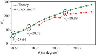
Figure 4: (color online) Experimentally measured and theoretically estimated angular Schmidt number $K_{a}$ versus $\theta_{p}$.

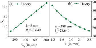
Figure 5: (color online) (a) and (b) Theoretical dependence of the angular Schmidt number on the width of the pump beam waist $w_{p}$ and crystal thickness $L$, respectively.

We find excellent agreement between the theory and experiment, except for extremely non-collinear conditions, in which case the experimentally measured Schmidt numbers are slightly lower than the theoretical predictions. The main reason for this discrepancy is the limited resolution of our EMCCD camera. In order to generate the azimuthal intensity plots, we use narrow angular region of interest (ROI) kulkarni2017natcomm , the minimum possible size of which is fixed by the pixel size of the EMCCD camera. In the case of non-collinear down-conversion, the intensities in the interferograms are concentrated at regions away from the center. Therefore, the corresponding $\Delta\bar{I}_{\rm out}(\phi)$ plots have lesser angular resolution and thus they get estimated to be wider than their true widths. This results in a progressively lower estimate of the Schmidt numbers with increasing non-collinearity. Finally, we use Eq. (9) for studying how $w_{p}$ and $L$ affect the angular Schmidt number $K_{a}$. Figure 5(a) shows the theoretical dependence of $K_{a}$ on $w_{p}$ for fixed $L$, $\theta_{p}$ and $d$. Figure 5(b) shows the theoretical dependence of $K_{a}$ on $L$ for fixed $w_{p}$, $\theta_{p}$, and $d$. We find that $K_{a}$ increases as a function of $w_{p}$ while it decreases as a function of $L$.

IV Conclusion

In summary, we have derived in this article an exact formula for the angular Schmidt spectrum of OAM-entangled photons produced by PDC. We have shown that our formula yields the true theoretical spectrum without any convergence issue as has been the case with the previously derived formulas. Furthermore, we have used our theoretical formulation to experimentally characterize the angular Schmidt spectrum for non-collinear phase matching in PDC. The results reported in this article can be very relevant for the ongoing intensive research efforts towards harnessing high-dimensional OAM entanglement for quantum information applications pors2011jo ; erhard2018lsa .

References

- (1) V. Karimipour, A. Bahraminasab, and S. Bagherinezhad, Phys. Rev. A 65, 052331 (2002).
- (2) N. J. Cerf, M. Bourennane, A. Karlsson, and N. Gisin, Phys. Rev. Lett. 88, 127902 (2002).
- (3) G. M. Nikolopoulos, K. S. Ranade, and G. Alber, Phys. Rev. A 73, 032325 (2006).
- (4) A. K. Jha, G. S. Agarwal, and R. W. Boyd, Phys. Rev. A 83, 053829 (2011).
- (5) D. Collins, N. Gisin, N. Linden, S. Massar, and S. Popescu, Phys. Rev. Lett. 88, 040404 (2002).
- (6) J. Leach, B. Jack, J. Romero, M. Ritsch-Marte, R. W. Boyd, A. K. Jha, S. M. Barnett, S. Franke-Arnold, and M. J. Padgett, Opt. Express 17, 8287 (2009).
- (7) T. Vértesi, S. Pironio, and N. Brunner, Phys. Rev. Lett. 104, 060401 (2010).
- (8) A. Vaziri, J.-W. Pan, T. Jennewein, G. Weihs, and A. Zeilinger, Phys. Rev. Lett. 91, 227902 (2003).
- (9) G. Molina-Terriza, A. Vaziri, R. Ursin, and A. Zeilinger, Phys. Rev. Lett. 94, 040501 (2005).
- (10) L. Allen, M. W. Beijersbergen, R. J. C. Spreeuw, and J. P. Woerdman, Phys. Rev. A 45, 8185 (1992).
- (11) S. M. Barnett and D. T. Pegg, Phys. Rev. A 41, 3427 (1990).
- (12) E. Yao, S. Franke-Arnold, J. Courtial, S. Barnett, and M. Padgett, Opt. Express 14, 9071 (2006).
- (13) C. K. Law and J. H. Eberly, Phys. Rev. Lett. 92, 127903 (2004).
- (14) J. P. Torres, A. Alexandrescu, and L. Torner, Phys. Rev. A 68, 050301 (2003).
- (15) F. M. Miatto, A. M. Yao, and S. M. Barnett, Phys. Rev. A 83, 033816 (2011).
- (16) A. M. Yao, New Journal of Physics 13, 053048 (2011).
- (17) A. K. Jha, G. S. Agarwal, and R. W. Boyd, Phys. Rev. A 84, 063847 (2011).
- (18) F. M. Miatto, H. D. L. Pires, S. M. Barnett, and M. P. van Exter, The European Physical Journal D 66, 263 (2012).
- (19) Y. Zhang and F. S. Roux, Physical Review A 89, 063802 (2014).
- (20) A. Mair, A. Vaziri, G. Weihs, and A. Zeilinger, Nature 412, 313 (2001).
- (21) J. B. Pors, S. S. R. Oemrawsingh, A. Aiello, M. P. van Exter, E. R. Eliel, G. W. ’t Hooft, and J. P. Woerdman, Phys. Rev. Lett. 101, 120502 (2008).
- (22) A. K. Jha, J. Leach, B. Jack, S. Franke-Arnold, S. M. Barnett, R. W. Boyd, and M. J. Padgett, Phys. Rev. Lett. 104, 010501 (2010).
- (23) W. H. Peeters, E. J. K. Verstegen, and M. P. van Exter, Phys. Rev. A 76, 042302 (2007).
- (24) H. Di Lorenzo Pires, H. C. B. Florijn, and M. P. van Exter, Phys. Rev. Lett. 104, 020505 (2010).
- (25) D. Giovannini, F. Miatto, J. Romero, S. Barnett, J. Woerdman, and M. Padgett, New Journal of Physics 14, 073046 (2012).
- (26) G. Kulkarni, R. Sahu, O. S. Magaña-Loaiza, R. W. Boyd, and A. K. Jha, Nature communications 8, 1054 (2017).
- (27) H. Qassim, F. M. Miatto, J. P. Torres, M. J. Padgett, E. Karimi, and R. W. Boyd, JOSA B 31, A20 (2014).
- (28) C. K. Hong and L. Mandel, Phys. Rev. A 31, 2409 (1985).
- (29) S. P. Walborn, C. Monken, S. Pádua, and P. S. Ribeiro, Physics Reports 495, 87 (2010).
- (30) L. Allen, M. W. Beijersbergen, R. J. C. Spreeuw, and J. P. Woerdman, Phys. Rev. A 45, 8185 (1992).
- (31) D. Eimerl, L. Davis, S. Velsko, E. Graham, and A. Zalkin, Journal of applied physics 62, 1968 (1987).
- (32) B.-J. Pors, F. Miatto, E. Eliel, J. Woerdman, et al., Journal of Optics 13, 064008 (2011).
- (33) M. Erhard, R. Fickler, M. Krenn, and A. Zeilinger, Light: Science & Applications 7, 17146 (2018).