Chaotic bursting in semiconductor lasers

Abstract

We investigate the dynamic mechanisms for low frequency fluctuations in semiconductor lasers subject to delayed optical feedback, using the Lang-Kobayashi model. This system of delay differential equations displays pronounced envelope dynamics, ranging from erratic, so called low frequency fluctuations to regular pulse packages, if the time scales of fast oscillations and envelope dynamics are well separated. We investigate the parameter regions where low frequency fluctuations occur and compute their Lyapunov spectrum. Using geometric singular perturbation theory, we study this intermittent chaotic behavior and characterize these solutions as bursting slow-fast oscillations.

I Introduction

In this paper, we theoretically investigate the phenomenon of low frequency fluctuations (LFF) Morikawa et al. (1976); Risch et al. (1977) in a semiconductor laser subject to delayed optical self-feedback. In the LFF regime, the laser electric field amplitude is bound by a low-frequency envelope that possesses amplitude dropouts at irregular times, i.e. the laser flickers. If these LFFs are approximately periodic, they are also referred to as regular pulse packages Heil et al. (2001); Davidchack et al. (2001)(RPP). To model the dynamics of semiconductor lasers with feedback, Lang and Kobayashi Lang and Kobayashi (1980) (LK) proposed the following system

$$E^{\prime}(t) = \left(1+i\alpha\right)N(t)E(t)+\eta e^{i\phi}E(t-\tau),$$ (1)

$$N^{\prime}(t) = \varepsilon\left[J-N(t)-\left(1+2N(t)\right)|E(t)|^{2}\right].$$ (2)

Equations (1)–(2) model the time-evolution of the laser in-cavity complex electric field $E(t)$ and excess carrier density $N(t)$. The parameter $\alpha$ is laser-specific, the so called linewidth enhancement factor, $\eta>0$ and $\phi\in\mathbb{R}$ are the strength and phase shift of the feedback electric field. The time-delay $\tau>0$ is the external cavity roundtrip time given in units of the photon lifetime, i.e. $\tau=T/\tau_{p}$ where $T$ is the roundtrip time and $\tau_{p}$ is the photon lifetime. The parameter $\varepsilon>0$ is the ratio of the photon and carrier lifetimes $\tau_{p}/\tau_{c}$, and it is usually a small parameter. $J$ is the excess pump current, i.e. without self-feedback, the solitary laser amplifies light when $J>0$.

Equations (1)–(2) are equivariant with respect to optical phase-shifts $\left(E,N\right)\rightarrow\left(e^{i\psi}E,N\right),\,\psi\in\mathbb{R}$. Therefore, they generically possess periodic solutions of the form $E(t)=re^{i\omega t},$ $N(t)=n,$ such that $r>0$ and $\omega,n\in\mathbb{R}$ satisfy

$$r = \sqrt{\frac{J-n}{1+2n}},$$ (3)

$$i\omega = \left(1+i\alpha\right)n+\eta e^{i\left(\phi-\tau\omega\right)},$$ (4)

referred to as External Cavity Modes (ECMs).

ECMs are shown to play an important role in shaping the dynamics of the LK system. In particular, a route to chaos has been shown via a period doubling cascade of ECMs as $\eta$ is increased, where the onset of chaos is related to the appearance of LFFs Ye, Li, and McInerney (1993); Hohl and Gavrielides (1999) and the chaotic attractor coexists with a stable ECM Mørk, Tromborg, and Mark (1992); Levine et al. (1995), the so-called maximum gain mode. It has been shown Lenstra (1991); Sano (1994); Van Tartwijk, Levine, and Lenstra (1995); Fischer et al. (1996) that LFFs can be considered as a chaotic itinerancy process on this attractor: An LFF solution ”hops” from one mode to another towards the maximum gain mode, until it gets close to the stable manifold of an ECM of saddle-type causing the LFF dropout event Lenstra (1991); Sano (1994); Van Tartwijk, Levine, and Lenstra (1995); Fischer et al. (1996). This mechanism in the LK model agrees with the experiments Fischer et al. (1996); Torcini et al. (2006). In view of the importance of the ECMs, their stability properties have been studied in detail in Refs. Wolfrum and Turaev, 2002; Rottschäfer and Krauskopf, 2007; Yanchuk and Wolfrum, 2010. Further increasing the feedback strength however, leads to extensive chaos, the so-called coherence collapse, without notable envelope dynamics Lenstra, Verbeek, and Den Boef (1985); Heil, Fischer, and Elsäßer (1999).

The structure of the paper is as follows. In Section II, we determine parameter values in the $(\varepsilon,\tau)$-parameter plane, where LFFs are observed numerically. Further, we study Lyapunov exponents Farmer (1982) (LE) of LFFs to quantify their chaotic behavior. In the particular case of large delay, it is useful to consider asymptotic properties of the Lyapunov spectrum leading to the distinction of weak versus strong chaos Heiligenthal et al. (2011, 2013); D’Huys, Jüngling, and Kinzel (2014); Jüngling, Soriano, and Fischer (2015); Yanchuk and Giacomelli (2017). For a superthreshold pump current, we show that the LFF corresponds to a weakly chaotic orbit exhibiting short events of intermittent strong chaos.

In the second part of the paper, Sec. III, we provide a complementary, geometric description of LFFs. For this, we discuss stability properties of the off-state $E(t)=0$ and provide a simple geometric viewpoint of the underlying dynamics for small $\varepsilon$. In particular, we characterize LFFs as slow-fast oscillations, which can be decomposed into pieces, each obtained from multiple time scale analysis as $\varepsilon\to 0$. We propose an averaged system of ODEs describing the fast oscillations between the dropout events. In addition, we describe the fast time-scale oscillations as interactions of eigen-modes of the off-state. As this phenomenon bares some resemblance to a class of slow-fast oscillations in neuronal systems modeled by ODEs Izhikevich (2000), we follow in notation and refer to them as bursting solutions.

II Parameter values where LFFs occur and properties of LFFs

II.1 Parameter region of LFFs

In this section, we numerically explore the parameter range where LFFs can be observed. Since it is not feasible to consider all five parameters in a numerical study, we fix $\alpha=5$, $\eta=0.1$, and $\varphi=0.5$ (see Ref. Torcini et al., 2006) and vary the parameters $\tau$, $\varepsilon$, and $J$. Note that the value of the feedback phase $\varphi$ does not play an essential role for the long-delay case, therefore, the observed results do not depend on the chosen value of $\varphi$, at least for large feedback delay $\tau$.

In order to quantify the dropout events, we introduce the probability $p$ for the solution to exhibit an amplitude dropout using the following empirical algorithm:
1. For a given solution, we consider the running average $\tilde{R}\left(t\right)$ of the laser field amplitude $\tilde{R}(t)=\int_{t-\tau}^{t}|E(\theta)|d\theta$ over a window of length $\tau$.
2. For a sufficiently long trajectory (here, we choose $10^{5}$ delay intervals, after some transient), we denote $\mathbb{P}(\{\tilde{R}\left(t\right)<\nu\})$ the probability of the laser amplitude to be below the threshold $\nu$.
3. We compute the conditional probability

$$p_{\nu_{1},\nu_{2}}:=\mathbb{P}_{\left\{\tilde{R}\left(t\right)<\nu_{2}\right\}}\left(\left\{\tilde{R}\left(t\right)<\nu_{1}\right\}\right)=\frac{\mathbb{P}\left(\left\{\tilde{R}\left(t\right)<\nu_{1}\right\}\right)}{\mathbb{P}\left(\left\{\tilde{R}\left(t\right)<\nu_{2}\right\}\right)}$$

for $\nu_{1}<\nu_{2}$, that is the fraction of time intervals, for which the field amplitude satisfies $\tilde{R}\left(t\right)<\nu_{1}$ provided it is below $\nu_{2}$. Intuitively speaking, $\nu_{1}$ determines the maximum value of $\tilde{R}(t)$, which we tolerate within a dropout event and $\nu_{2}$ specifies the minimum value of $\tilde{R}(t)$, we require outside of a dropout event. The optimal choice of these threshold values is empiric. By experimenting and testing the known LFF regimes, we set the values to $\nu_{1}=0.1$ and $\nu_{2}=0.3$ (see Fig. 1).
4. Finally, we would like to discard the solutions that are oscillating around the zero-amplitude threshold, since they are clearly not LFFs. Therefore, we define the measure

$$p:=p_{\nu_{1},\nu_{2}}\frac{N_{\nu_{2}}}{N_{\nu_{1}}},$$

where $N_{\nu}$ is the number of crossings of the corresponding threshold value $\nu$. In the case when the solution possesses fast oscillations around $\nu_{1}$ within one dropout event, the value of $N_{\nu_{1}}/N_{\nu_{2}}$ is large and, hence, the measure $p$ attains small values.

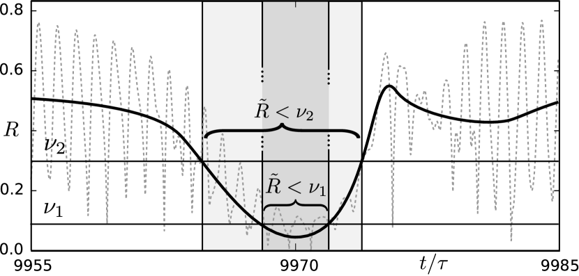
Figure 1: Visual guidance for the computation of the measure $p$. The figure shows the amplitude $R(t)$ (gray, dotted) of a solution segment of Eqs. (1)–(2) for $9955<t/\tau<9985$ and the parameters $\alpha=5$, $\eta=0.1$, $\phi=0.5$, $\varepsilon=0.003$, and $\tau=100$. In a dropout event, the time-$\tau$ averaged amplitude $\tilde{R}(t)$ (black, solid) falls below the threshold values $\nu_{1}=0.1$, $\nu_{2}=0.3$, respectively. The exact definition of $p$ (and $\tilde{R}$) is given in the text.

It is clear that such a defined quantity $p$ is largest if all dropouts below the threshold $\nu_{2}$ attain almost only values smaller than $\nu_{1}$. Hence, the higher values of $p$ are indicators of an orbit to posses a dropout event, and, therefore, it is a candidate for LFFs or RPPs. Here we should note that the values of $p$ close to 1 can also indicate a high degree of regularity or simply convergence to $E(t)=0$. For instance, for a rectangular piecewise constant (square wave) function with two values $\tilde{R}_{1},\tilde{R}_{2}$, $\tilde{R}_{1}<\nu_{1}<\nu_{2}<\tilde{R}_{2}$, the value of $p$ equals $1$. However, these parameter regimes have been avoided carefully.

Using the introduced quantity $p$, Fig. 2 shows the regions for the existence of LFFs with respect to parameters $J$, $\varepsilon$, and $\tau$. In Fig. 2(a), we fix parameters $\varepsilon=0.03,~{}\eta=0.1,~{}\alpha=5$, for which LFFs have been reported experimentally in Ref. Torcini et al., 2006. For this choice of parameters, LFFs do not appear for small values of the time-delay, $\tau<40$. Moreover, LFFs cease to exist for large values of $\tau$. In the $(J,\tau)$ parameter plane, $p$ attains its maximum for $J\approx 0$ and $\tau\approx 85$. The corresponding solution for maximal $p$ is shown in Fig. 2(b) and displays pronounced LFFs.

In order to investigate the interplay of $\varepsilon$ and $\tau$, we fix the maximum-$p$ delay value $\tau=85$ and investigate the influence of the parameter $\varepsilon\tau$ on the occurrence of LFFs. Note that $\varepsilon\tau=T/\tau_{c}$ is the external cavity roundtrip time given in units of the carrier lifetime. For the maximum-$p$ solution shown in Fig. 2(b), we have $\varepsilon\tau\approx 2.6$. We fix this relation when changing $\tau$ in Fig. 2(c). More specifically, Fig. 2(c) shows the same as (a) but with variable $\varepsilon=2.6/\tau$, as we vary the delay. One observes clearly that LFFs are more abundant in Fig. 2(c).

Figure 2(d) shows the value of $p$ in the parameter plane $(J,\log\varepsilon)$ with fixed $\tau=85$. We observe two distinct parameter regions, where $p$ attains high values. In the dark region located in the upper part of Fig. 2(d), $\varepsilon\tau\in[1.7,2.7]$, we observe LFFs. The lower parameter region in Fig. 2(d) corresponds to RPP solutions (Fig. 2(e)), which have been reported in Refs. Heil et al., 2001; Davidchack et al., 2001. It is characterized by the values $\varepsilon\ll 1$ and $\varepsilon\tau<1$.

Summarizing, Fig. 2 shows parameter regions where LFFs and RPPs are observed. These numerical results indicate the importance of $\varepsilon\tau$ as a scaling parameter. Moreover, we observe a clear distinction between LFFs and RPPs, namely, the LFFs are observed for $\varepsilon\tau>1$ and RPPs for $\varepsilon\tau<1$ with a clear gap between them, at least when the other parameters $\eta,\phi,\alpha$ are chosen as mentioned above.

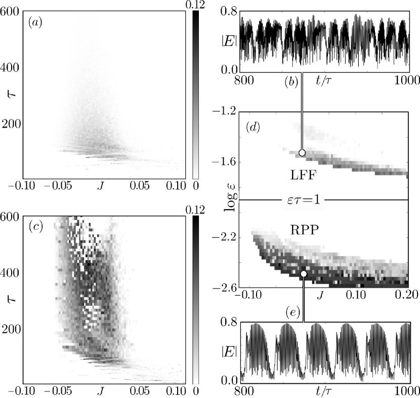
Figure 2: Parameter ranges, where LFFs and RPPs are observed. Parameter $(J,\tau)$-diagram in panel (a) shows the probability $p$ for the occurrence of LFFs (see the description of $p$ in the text) for all other fixed parameters $\varepsilon=0.03$, $\eta=0.1$, $\alpha=5$. Panel (c) shows the same as (a) but with variable $\varepsilon=2.6/\tau$. One observes that LFFs are more abundant in (c), where $\varepsilon$ is scaled with $\tau$. Panel (d) shows the same LFF indicator in the parameter plane $(J,\log\varepsilon)$ with fixed $\tau=85$. Two distinct parameter regions are observed: one for LFFs and another for RPPs existing for significantly smaller values of $\varepsilon$, such that $\varepsilon\tau<1$. Panels (b) and (e) illustrate trajectories from the corresponding parameter regions of (d).

II.2 Lyapunov Spectrum

In this section, we provide a detailed analysis of the Lyapunov Spectrum of LFFs. We briefly introduce some necessary concepts. Let $\left(E\left(t\right),N\left(t\right)\right)$ be a solution to Eqs. (1)–(2) and consider $\xi\left(t\right)$ the solution of the linearized equation

$$\xi^{\prime}\left(t\right)=A(t)\xi\left(t\right)+B(t)\xi\left(t-\tau\right)$$

along the solution $\left(E\left(t\right),N\left(t\right)\right)$. Here $f(\cdot)$ is the right-hand side of Eqs. (1)–(2), and $A(t):=Df\left(E\left(t\right),N\left(t\right),E(t-\tau)\right)$ and $B(t):=D_{\tau}f\left(E\left(t\right),N\left(t\right),E(t-\tau)\right)$ denote the Jacobians with respect to non-delayed and delayed arguments, respectively. The Lyapunov Exponent Farmer (1982)(LE) is defined as

$$\lambda=\limsup_{t\to\infty}\frac{1}{t}\log\|\xi\left(t\right)\|.$$

It is convenient to consider a related concept, the so called instantaneous or sub-LE, which is defined as

$$\sigma=\limsup_{t\to\infty}\frac{1}{t}\log\|\zeta\left(t\right)\|,$$

where $\zeta\left(t\right)$ is the solution to the truncated linearized equation $\zeta^{\prime}\left(t\right)=A(t)\zeta\left(t\right).$ The instantaneous LE can be used to distinguish the two distinct chaotic regimes of weak and strong chaos Heiligenthal et al. (2011, 2013); Jüngling, Soriano, and Fischer (2015); Yanchuk and Giacomelli (2017). In particular, we call strong chaos, when the instantaneous LE is positive, while weak chaos is characterized by negative instantaneous LE and positive LE.

We have computed the largest LE and the instantaneous LE of solutions to Eqs. (1)–(2) for varying values of the pump current $J$ and different values of delay $\tau$ in Fig. 3. From left to right, we observe a convergence to the off-state ($J<-\eta=-0.1$), weak chaos ($-0.1<J<0.06$), and strong chaos ($J>0.06$). In the regime of weak chaos we observe $\lambda\sim 1/\tau$. Indeed, we have computed the ten largest LEs for fixed $J=-0.05$ for varying delay time $\tau$ in Fig. 3(inset II) to show this scaling property. Contrarily, in the case of strong chaos, $\lambda_{\max}\to\sigma$ as $\tau\to\infty$, where $\lambda_{\max}$ is the largest LE. Fig. 3 shows that for $J=0.07$ the largest LE remains at constant positive values as the delay increases.

When comparing the domain of existence of LFFs in Fig. 2(a) with Fig. 3 (both figures computed for $\varepsilon=0.03$), we see that LFFs occur in the regime of weak chaos, at least those shown in Fig. 2(a). However, this observation should be considered with caution, since LFFs cease to exist for fixed $\varepsilon$ and very large $\tau$, as follows from Sec. II.1. Hence, one cannot identify an appropriate LFF-trajectory asymptotically for $\tau\to\infty$ (and all other parameters fixed), as one would need for weak chaos. Nevertheless, an approximate description can be done still for the reported values of $\tau$ that are of order $10^{3}$.

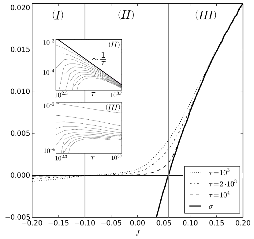
Figure 3: Scaling behavior of Lyapunov Exponents (LE) for fixed values $\varepsilon=0.03,$ $\eta=0.1,$ and $\alpha=5$. The figure displays the largest LE $\lambda_{\max}$ for different values of the pump current $J\in[-0.2.0.2]$ and three fixed values of the time-delay $\tau\in\left\{10^{3},2\cdot 10^{3},10^{4}\right\}$. The respective largest instantaneous LEs $\sigma$ coincide for all considered values of $\tau$. We obtain 3 distinct regimes. (I): convergence to equilibrium, (II): weak chaos ($\lambda=\mathcal{O}\left(1/\tau\right)$ as $\tau\to\infty$), (III): strong chaos ($\lambda=\mathcal{O}\left(1\right)$ as $\tau\to\infty$). To visualize the scaling behavior of $\lambda_{\max}$, the 10 largest LE for $J=-0.05$ (II) and $J=0.07$ (III) are provided in the insets in log-log plot.

A better understanding of the finite-time LEs can be achieved by considering $E\left(t\right)$ as a time series given by the solution to the nonautonomous system (1). Then, the instantaneous LE of it, can be obtained from the truncated system

$$E^{\prime}(t)=(1+i\alpha)N(t)E(t),$$ (5)

where $N(t)$ is a solution of the full LK system. Equation (5) is linear in $E$, hence, its instantaneous LE $\sigma_{E}$ is given by

$$\sigma_{E}=\limsup_{t\to\infty}\frac{1}{t}\int_{0}^{t}N\left(s\right)\text{d}s.$$ (6)

In particular, this simple computation reveals that the onset of strong chaos is due to positive values of $N\left(t\right)$. In particular, if $N\left(t\right)\geq 0$ for some time-interval, it gives rise to a positive instantaneous finite time LE, that is the instantaneous local rate of the growth at time $t$: $\sigma_{E,loc}(t)=\frac{1}{l}\int_{t-l}^{t}N\left(s\right)\text{d}s$ for certain $t$ and $l$. In the case $J>0$ and considering an LFF trajectory, the positive values of $N(t)$ are observed during the dropouts, see Fig. 4. This is very intuitive as $N(t)>0$ corresponds to the light amplification regime of the laser without feedback.

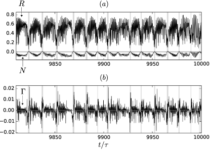
Figure 4: Panel (a): Time series of amplitude $R(t)=|E(t)|$ and carrier density $N(t)$ of a solution to LK for fixed parameters $\alpha=5,\eta=0.1,\phi=0.5,\varepsilon=0.025,$ and $J=0.02.$ The intervals, where $N(t)\geq 0$, are highlighted by vertical gray lines with the width corresponding to the duration of the event. These intervals clearly indicate the LFF dropout event. Panel (b): Exponential rate of change of the amplitude $\Gamma(t)=\log(R(t)/R(t-\tau))/\tau$ from one delay interval to the next. LFFs dropout events are characterized by larger values of $\Gamma(t)$, as the solution changes fast between delay intervals.

III Chaotic Bursting

In this section, we propose a description of a mechanism responsible for LFFs in the LK model using singular geometric perturbation theory. We describe how LFFs can be viewed as a sequence of slow and fast solution segments obeying a reduced set of equations. In particular, we reveal how the increasing values of $N(t)$ lead to the dropout and how the solution bursts off the non-lasing state $E(t)=0$. In addition, we propose an averaged system of ODEs describing the intermediate fast oscillations between the dropouts events for small $\varepsilon$.

At first, we go through the stability analysis of the off-state $E(t)=0$. Secondly, we investigate the limit $\varepsilon\to 0$ and appeal to invariant manifolds theory to provide a geometric understanding of LFF (and RPP) events. As we intent to get across the main idea and provide the underlying mechanism, we leave out the technical details. We refer to Refs. Bates, Lu, and Zeng, 1998, 2000 for the theory of invariant manifolds for semiflows. Via averaging, we obtain a related ODE system and perform a slow-fast analysis of this system. We show how the fast time-scale oscillations result from the dynamics residing close to eigen-modes of the equilibrium $E(t)=0$ as long as it is stable (in this average sense) and ”hop” to another when it becomes unstable, thereby revealing the mode-hopping mechanism.

III.1 Stability of the off-state

The linear stability of the steady state $(E(t),N(t))=(0,J)$ can be obtained from the corresponding linearized system

$$E^{\prime}\left(t\right) = \left(1+i\alpha\right)nE\left(t\right)+\eta e^{-i\phi}E\left(t-\tau\right),$$ (7)

$$N^{\prime}\left(t\right) = -\varepsilon N,$$ (8)

where $n=J$ is the equilibrium value of $N(t)$. We use a new notation $n$ instead of $J$ for the equilibrium value of $N$, since the results obtained in this section will be useful also in the subsequent Sec. III.2, where $N(t)$ will admit also other values different from $J$.

Equations (7)—(8) are decoupled and, in $N$-direction, the eigenvalue is $\lambda=-\varepsilon$. The remaining spectrum consists of eigenvalues $\lambda$, which are solutions of the characteristic equation

$$-\lambda+\left(1+i\alpha\right)n+\eta e^{-i\phi-\tau\lambda}=0$$ (9)

obtained by inserting the ansatz $E(t)=E(0)e^{\lambda t}$ into Eq. (7). The equilibrium is stable, if all eigenvalues have negative real parts.

Firstly, let us note that the equilibrium is stable for $n<-\eta$. This can be easily seen from the real part of the characteristic equation (9)

$$\mbox{Re}\lambda=n+\eta e^{-\tau\mbox{Re}\lambda}\cos(\phi+\tau\mbox{Im}\lambda),$$

which can be estimated as $\mbox{Re}\lambda\leq n+\eta$ for all $\lambda$ such that $\mbox{Re}\lambda\geq 0$ and $\eta>0$. Note that, generically, $\lambda=0$ is not an eigenvalue, since $\lambda=0$ implies $\phi=\arctan\alpha+2k\pi,~{}k\in\mathbb{Z},$ which is a special case not considered here.

Therefore, the equilibrium may destabilize via a bifurcation of Hopf-type, where a purely imaginary eigenvalue $\lambda=i\omega$ crosses the imaginary axis and gives rise to an ECM solution with period $2\pi/\omega$. These Hopf bifurcation curves are shown in Fig. 5. The diagram can be interpreted as follows. First, for every fixed $n$ there are values $\tau_{0}(n),\tau_{1}(n),\dots$ such that a purely imaginary eigenvalue crosses the imaginary axis. Secondly, for every fixed $\tau$, there are $n_{0}=n_{0}(\tau,\omega_{0}),~{}n_{1}=n_{1}(\tau,\omega_{1}),\dots$ such that there exist ECMs with periods $2\pi/\omega_{0},~{}2\pi/\omega_{1},\dots~{}$, if $n_{0}=n_{0}(\tau,\omega_{0}),~{}n_{1}=n_{1}(\tau,\omega_{1}),\dots<J$. Fig. 5 shows the stability region of the off-state and illustrates that the number of ECMs grows proportionally with the time-delay.

As a next step, we discuss how large the critical eigenvalues are. More specifically, we are interested in scaling properties of the eigenvalues for large delay. Accordingly to the theory in Ref. Lichtner, Wolfrum, and Yanchuk, 2011 (see also reviews in Refs. Yanchuk and Giacomelli, 2017; Wolfrum et al., 2011), the eigenvalues scale generically either as $1/\tau$ for large $\tau$ (weak instability) or as $\mathcal{O}(1)$ (strong instability), similarly to the scaling of LEs for weak and, respectively, strong chaos discussed in Sec. II.2. Both parts of the spectrum can be calculated. We omit here the details of the straightforward calculations (see e.g. Refs. Lichtner, Wolfrum, and Yanchuk, 2011; Yanchuk and Giacomelli, 2017; Wolfrum et al., 2011), and present the results. In particular, the strong spectrum is given by

$$\lambda_{\mbox{strong}}\approx(1+i\alpha)n,\quad\mbox{for}\quad n>0$$ (10)

and the weak spectrum can be approximated by the continuous curve

$$\lambda_{\mbox{weak}}(\omega)=\frac{1}{\tau}\gamma(\omega)+i\omega=-\frac{1}{2\tau}\ln\frac{\left(\omega-\alpha n\right)^{2}+n^{2}}{\eta^{2}}+i\omega,$$

$\omega\in\mathbb{R},$ as $\tau\to\infty$. If $n<0$, the strong spectrum is absent and there is no positive eigenvalue with $\mbox{Re}\left(\lambda\right)=\mathcal{O}(1)$ as $\tau\to\infty$. Then, the largest real parts of eigenvalues are approximately given by

$$\max_{\omega}\mbox{Re}(\lambda)\approx\max_{\omega}\frac{\gamma(\omega)}{\tau}=\frac{\gamma(\alpha n)}{\tau}=\frac{1}{\tau}\ln\left|\frac{\eta}{n}\right|.$$ (11)

Therefore, for large values of $\tau$ and $-\eta<n<0$, $E(t)=0$ is so-called weakly unstable with the most unstable eigen-mode $e^{i\alpha nt}$. If $n>0$, we call $E(t)=0$ strongly unstable, with most unstable eigen-mode $e^{\left(1+i\alpha\right)nt}$.

Figure 5: Stability of the off-state $E(t)=0$. The figure shows the Hopf bifurcation curves in the parameter plane $(n,\tau)$, $n\in[-0.2,0.2]$, $\tau\in[0,100]$ for the fixed parameter values $\alpha=5,~{}\eta=0.1,\phi=0.5$, and $\varepsilon$ arbitrary (stability does not depend on $\varepsilon>0$). Here, $n$ is the equilibrium value of the $N$-variable. $E(t)$ is stable independently on $\tau$, when $n<-\eta=-0.1$. As $n$ increases one pair of eigenvalues crosses the imaginary axis at each Hopf bifurcation curve.

III.2 Direct slow-fast analysis

In this section, we present a mechanism for the recurrent appearance of dropouts during LFFs. For this we use a direct slow-fast analysis and smallness of parameter $\varepsilon$. We split the description into two parts: Part 1 describes the dynamics close to the off-state and the mechanisms that bound the orbit close to the off-state for certain time and then leads to the amplitude increase, i.e. repelling from the off-state. Part 2 describes the return mechanism for solutions with large amplitude. The LFF recurrent mechanism then follows from the combination of these two ingredients.

Part 1. Dynamics close to the off-state, repelling mechanism.

Setting formally $\varepsilon=0$ in Eqs. (1)–(2), we obtain

$$E^{\prime}(t) = \left(1+i\alpha\right)N(t)E(t)+\eta e^{i\phi}E(t-\tau),$$ (12)

$$N^{\prime}(t) = 0,$$ (13)

hence, one can consider Eq. (12) in a layer given by a fixed value $n=N\left(0\right)$. As a result, we obtain Eq. (7), which was studied in the previous section in detail. In particular, $E(t)=0$ is an equilibrium for every $n\in\mathbb{R}$. In other words, system with $\varepsilon=0$ possesses the line of equilibria $M=\{(E,N)=(0,n)\,|\,n\in\mathbb{R}\}$.

The invariant line $M$ (or any connected compact subset of it) is called normally hyperbolic, if the characteristic equation (9) has no solutions $\lambda=\lambda(n)$ with zero real part. Normal hyperbolicity ensures persistence of $M$ under small perturbations Bates, Lu, and Zeng (1998, 2000). As follows from Sec. III.1, for every $\tau$ there exists $n^{\ast}(\tau)\geq-\eta$ such that for $n<n^{\ast}(\tau)$, the line of equilibria parametrized by $n$ is normally exponentially stable with uniform bounds away from $n^{\ast}(\tau)$ (and unstable otherwise), see Fig. 5, where $n^{*}(\tau)$ is the stability boundary.

In order to reveal the slow dynamics on $M$, we rescale time as $\tilde{t}=\varepsilon t$ in Eqs. (1)–(2) and obtain

$$\varepsilon\dot{E}(\tilde{t}) = \left(1+i\alpha\right)N(\tilde{t})E(\tilde{t})+\eta e^{i\phi}E(\tilde{t}-\varepsilon\tau),$$ (14)

$$\dot{N}(\tilde{t}) = \left[J-N(\tilde{t})-\left(1+2N(\tilde{t})\right)|E(\tilde{t})|^{2}\right],$$ (15)

where the dot denotes differentiation with respect to the new slow time. Considering the limiting case $\varepsilon=0$ and $E(t)=0$, it is easy to see that the slow flow on $M$ is given by the ODE $\dot{N}(\tilde{t})=J-N(\tilde{t}),$ with the stable equilibrium $N(\tilde{t})=J$. The above facts allow the description of the dynamical picture for small $\varepsilon$. We refer the reader to Fig. 6 for a visualization of the following paragraph.

Assume that at some point of time $N(t)=n<-\eta$ holds. Then, as follows from Sec. III.1, the zero equilibrium of the layer equation (12) is globally stable and, hence, the solution converges to the off-state $E(t)=0$, i.e. the point ($E(t)=0,N(t)=n$) on the invariant line $M$, see segment (A) in Fig. 6.

On the manifold $M$, the solution slowly (accordingly to the timescale $\tilde{t}=\varepsilon t$) moves towards the point $N(\tilde{t})=J$, $E(t)=0$ which is the stable equilibrium within $M$, see segment (B) in Fig. 6. In the case, when $J<n^{*}(\tau)$, the solution just converges to the stable off-state. However, for the LFF case, it holds $J>n^{*}(\tau)$. Hence, as the value of $N(\tilde{t})$ increases, $M$ loses normal stability at $n^{\ast}(\tau)$, and it causes $R(t)=|E(t)|$ to increase with the approximate rate $\frac{1}{\tau}\ln(\left|\eta/N(\tilde{t})\right|)$ (see Eq. (11)) when $N(\tilde{t})<0$, see segment (C) in Fig. 6. For large $\tau$, this rate of increase can be very slow, and, in particular, the interplay between $\varepsilon$ (speed of the motion along $M$) and $1/\tau$ (repelling rate) can play a decisive role in determining the time the solution spends in the vicinity of the off-state. Moreover, if $J>0$, then $N(\tilde{t})$ can become positive, which leads to even faster repelling rate, see Eq. (10), that is independent of $\tau$, see segment (C’) in Fig. 6. The above mechanism describes the attraction by and repelling from the off-state, which determines the dropout event

Part 2. Return mechanism for large-amplitude solutions.

Note that for values

$$R(t)>\sqrt{\frac{J-N(t)}{1+2N(t)}}$$

it holds $N^{\prime}(t)<0$ and $N(t)$ is strictly decreasing. This leads to a return to smaller values of $N(t)$. Indeed, as soon as $N<n^{*}(\tau)$, the equilibrium in the layer equation of $E(t)$ becomes again stable and the solution converges back to the off-state, see segments (D) and (A) in Fig. 6.

The return mechanism can be explained more rigorously for the case when the amplitude $R$ becomes large. For instance, let us assume that $R\left(t\right)\approx 1/\sqrt{\varepsilon\tau},$ then the rescaled variable $\tilde{E}(t)=\sqrt{\varepsilon\tau}E(t)$ can be introduced, and the resulting system has the form of the perturbed equation

$$\tilde{E}^{\prime}\left(t\right) = \left(1+i\alpha\right)N\left(t\right)\tilde{E}\left(t\right)+\eta e^{i\phi}\tilde{E}\left(t-\tau\right),$$ (16)

$$N^{\prime}\left(t\right) = -\frac{1}{\tau}\left(1+2N\left(t\right)\right)\left|\tilde{E}\left(t\right)\right|^{2}+\varepsilon\left(J-N\left(t\right)\right).\qquad$$ (17)

Since $J-N\sim\eta$, the term $\varepsilon\left(J-N\left(t\right)\right)\sim\varepsilon\eta$ is smaller than $1/\tau$ for the parameters considered. Hence, by neglecting this term, it follows that $N^{\prime}\left(t\right)\leq 0$ and $N\left(t\right)\to-1/2<-\eta$ as $t\to\infty$. As a result, $\tilde{E}\left(t\right)\to 0$ as $t\to\infty$. In particular, $\tilde{E}(t)$ decreases until the rescaling is not justified anymore with some value $N\left(t\right)=n$. If again $n<n^{\text{$\ast$}}(\tau)$, $E(t)=0$ is stable in this layer and by the fast flow, the solution converges to $E(t)=0$ and we obtain the recurrent LFF behavior combining the mechanisms described in part 1 and part 2 above. Solutions that enter the regime of small amplitude for values $N(t)=n>n^{\text{$\ast$}}(\tau)$ however, do not fit this simple description. The equilibrium here is of (high-dimensional) saddle type, so that very complicated dynamics may arise.

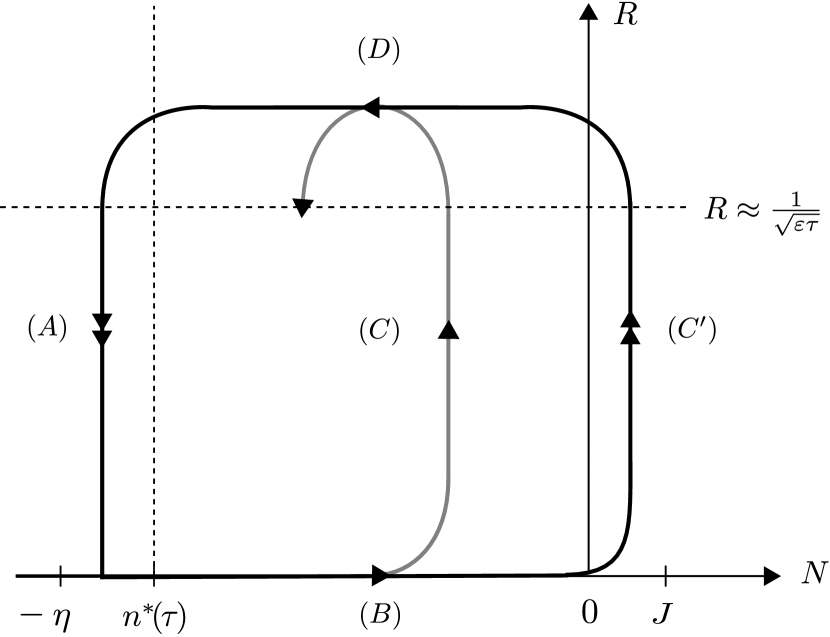
Figure 6: Slow-fast solution segments for $\varepsilon$ small. Fast segment (A): for $N(t)<n^{\ast}(\tau)$ the solution is attracted by the zero solution $R(t)=0$. Slow segment (B): for $N(t)<n^{\ast}(\tau)$ the solution stays close to $R(t)=0$ and $N(t)$ slowly increases towards $N(t)=J$. Segment (C): for $n^{\ast}(\tau)<N(t)<0$ and $\tau$ large, $R(t)$ increases slowly for large $\tau$ with the rate of increase bounded by $-\ln|n/\eta|/(2\tau)$. $R^{\prime}(t)=0$ in each layer containing an ECM. Fast segment (C’): For $N(t)>0$ the amplitude increases fast. Return flow (D): If $R(t)\geq 1/\sqrt{\tau\varepsilon}$, $N(t)$ is strictly decreasing for the considered parameters. See Sec. III.2 for details on black segments and Sec. III.4 for details on gray segments.

III.3 Averaging the fast flow

In order to describe the fast oscillatory behavior of the solution when $-\eta<n^{\ast}(\tau)<N(t)<0$, for $\eta$ small, in this section, we propose an averaging method leading to a system of ODEs. We define the exponential change rate of $E(t)$ between two subsequent delay intervals as

$$\Lambda\left(t\right):=\frac{1}{\tau}\mbox{Log}\left(\frac{E\left(t\right)}{E\left(t-\tau\right)}\right),$$ (18)

such that $E(t)=E(t-\tau)e^{\tau\Lambda(t)}$ and denote $\Gamma(t):=\mbox{Re}(\Lambda(t))$. Straightforward computation reveals that

$$\limsup_{L\to\infty}\frac{1}{L}\sum_{l=0}^{L}\Gamma\left(t_{0}+l\right)=\lambda_{E},$$

for all $t_{0}\geq 0$, where $\lambda_{E}$ is the LE of the E-variable, determined from of Eq. (1) only. Therefore $\Gamma\left(t\right)$ can be interpreted as a finite time LE Kanno and Uchida (2014) restricted to the $E$-component of the LK-system. Clearly, positivity of this LE implies positivity of a LE in the full system. $\Lambda(t)$ satisfies

$$\tau\Lambda^{\prime}\left(t\right)=\frac{E^{\prime}(t)}{E(t)}-\frac{E^{\prime}(t-\tau)}{E(t-\tau)},$$ (19)

where

$$\frac{E^{\prime}(t)}{E(t)}=(1+i\alpha)N(t)+\eta e^{i\phi-\tau\Lambda(t)}.$$ (20)

As $|N(t)|<\eta$ and, moreover, suggested by numerics, the assumption $\tau\mbox{Re}(\Lambda(t))\sim 1$ (see, e.g. Fig. 4(b)) leads to the estimate

$$\left|\frac{E^{\prime}(t)}{E(t)}\right|\leq C\eta.$$

As a result, the right hand side of Eq. (19) is bounded by $2C\eta$, where $C$ is independent of $\eta$. Hence, we can consider $h(t)={E^{\prime}(t-\tau)}/{E(t-\tau)}\sim\eta$ as a time-dependent small perturbation and replace it by its average over length $\tau$

$$\frac{1}{\tau}\int\limits_{0}^{\tau}h(t+s)ds=\frac{1}{\tau}\int\limits_{0}^{\tau}\frac{E^{\prime}\left(t+s-\tau\right)}{E\left(t+s-\tau\right)}ds=\Lambda\left(t\right).$$ (21)

to obtain the following ODE

$$\tau\Lambda^{\prime}\left(t\right)=\frac{E^{\prime}(t)}{E(t)}-\Lambda\left(t\right).$$ (22)

Using this ODE, one can express $R(t)$ as a function of $\Gamma(t)$. For this, by integrating (22) and taking the absolute value, we obtain

$$R(t)=R(0)\exp\left[\tau\left(\Gamma(t)-\Gamma(0)\right)+\int_{0}^{t}\Gamma(s)ds\right].$$ (23)

Now, substituting (20) into (22), and combining with (2), we derive the following system for $\Lambda(t)$ and $N(t)$

$$\tau\Lambda^{\prime}\left(t\right) = \left(1+i\alpha\right)N\left(t\right)+\eta e^{i\phi}e^{-\tau\Lambda\left(t\right)}-\Lambda\left(t\right),$$ (24)

$$N^{\prime}\left(t\right) = \varepsilon\left[J-N\left(t\right)-\left(1+2N\left(t\right)\right)R^{2}\left(t\right)\right],$$ (25)

where $R(t)$ is given by (23). The equation for $R$ can be also written in a differential form

$$R^{\prime}\left(t\right)=\left(N\left(t\right)+\eta e^{-\tau\Gamma\left(t\right)}\cos\left(\tau\Omega\left(t\right)-\phi\right)\right)R\left(t\right),$$ (26)

thus, completing the system (24)–(26). The right hand side of each equation satisfies the following order estimates $\Lambda^{\prime}\lesssim\eta/\tau$, $N^{\prime}\lesssim\varepsilon$, and $R^{\prime}\lesssim\eta$. In our case, all three estimations are small, which are the necessary conditions for the application of the averaging, and which ensure a certain closeness of the solutions of the averaged system (24)–(26) and the corresponding quantities $\Lambda(t)$, $R(t)$, and $N(t)$ obtained from the solutions $E(t)$ and $N(t)$ of the original LK system using the relations (22) and $R(t)=|E(t)|$. The in-depth analysis of the closeness of the solutions to averaged system and the LK system is very technical and out of the scope of this manuscript. Instead, in the next section, we study the averaged system for small $\varepsilon$.

III.4 Slow-fast analysis of the averaged system

We start with the limit $\varepsilon=0$, where the equations in a layer $N(t)=n$ of the averaged system (24)–(26) are given by

$$\tau\Lambda^{\prime}\left(t\right) = \left(1+i\alpha\right)n+\eta e^{i\phi}e^{-\tau\Lambda\left(t\right)}-\Lambda\left(t\right),$$ (27)

$$R^{\prime}\left(t\right) = \left(n+\eta e^{-\tau\Gamma\left(t\right)}\cos\left(\tau\Omega\left(t\right)-\phi\right)\right)R\left(t\right).\quad$$ (28)

Note that Eq. (27) is decoupled and does not depend on $R(t)$. One of the remarkable features of this system is that its equilibria $\Lambda(t)=\lambda$ satisfy Eq. (9), that is, the equilibria coincide with the eigenvalues of the characteristic equation for the off-state. Generically, there are countably many equilibria, since (9) is a quasi-polynomial. For a detailed analysis of Eq. (9), see Sec. III.1.

We linearize Eqs. (27)–(28) at such an equilibrium, where $\Lambda(t)=\lambda$ and $R(t)=0$. As Eq. (27) is decoupled, it is easy to check that the corresponding eigenvalues are given by $\mu_{1}=(1+i\alpha)n-\lambda-1/\tau$ and $\mu_{2}=\gamma$, where $\gamma=\mbox{Re}(\lambda)$. Thus, at $\gamma=0$, a simple, real eigenvalue crosses the imaginary axis. Moreover, $\mu_{1}$ crosses the imaginary axis at $\gamma_{H}=n-1/\tau$. To sum up, all equilibria $\lambda=\gamma+i\omega$ satisfying $\gamma_{H}<\gamma<0$ are stable, and unstable for $\gamma>0$ or $\gamma<\gamma_{H}$.

It is interesting that these equilibria correspond to the eigen-modes $E(t)=e^{\lambda t}$ of Eq. (7). In particular, we have shown that eigen-modes, which cause the amplitude of the electric field to increase $(\gamma>0)$ are unstable in the average sense above.

Similarly to Sec. III.2, these results hold for an arbitrary $n$, such that we obtain countably many curves of equilibria $\lambda=\lambda(n)$ across layers, and each of these curves is normally exponentially stable if $n-1/\tau<\mbox{Re}\left(\lambda\left(n\right)\right)<0$, with uniform bounds away from $n-1/\tau$ and 0. Hence, each of these normally exponentially stable pieces of the curves persist as invariant manifolds for $\varepsilon>0$. In order to obtain the slow flow on these curves, we rescale time as $\tilde{t}=\varepsilon t$ and consider the limit $\varepsilon=0$, to find that in the limit $\dot{N}(\tilde{t})=J-N(\tilde{t})$, see similar calculations in Sec. III.2. Hence, the solution follows the slow manifold close to $(\Lambda=\lambda(n),R=0,N=n)$ with increasing $n$ until it destabilizes or reaches $N=J$.

We remark, that Eqs. (27)–(28) attain a second set of equilibrium solutions $(\Lambda=i\omega,R=\mbox{const},N=n)$, where the value of $R$ is arbitrary and $\omega$, $N(t)$ satisfy Eq. (4). These correspond to the invariant co-rotating frames in the limit $\varepsilon=0$ for the original Eqs. (1)–(2), each containing one ECM. Note however, that these curves are not normally hyperbolic and hence, they do not persist for $\varepsilon>0$.

In the following paragraph we describe the mechanism of slow-fast oscillations in system (24)–(26) using similar arguments as in Sec. III.2. Assume that at some point of time $N(t)-1/\tau<\Gamma(t)<0$, with $N(t)=n$ holds. Then, the solution converges fast to a stable equilibrium $\lambda(n)$, $E(t)=0$, i.e. a point on the invariant curve $\left\{n\in\mathbb{\mathbb{R}}|\Lambda(t)=\lambda(n),E(t)=0,N(t)=n\right\}$, see segment (A) in Fig. 7. $\lambda\left(N(\tilde{t})\right)$ then evolves according to the slow flow on $\lambda(n)$, see segment (B) Fig. 7. If, as $N(\tilde{t})$ increases by the slow flow along $\lambda\left(N(\tilde{t})\right)$, $\lambda\left(N(\tilde{t})\right)$ destabilizes, $R\left(t\right)$ increases fast, see segment (C) in Fig. 7. There are no further equilibria in a layer, so we construct a return flow similar to Sec. III.2. As $R\left(t\right)$ increases, we can rescale $\tilde{R}(t):=R(t)/\sqrt{\varepsilon\tau}$. When $\tilde{R}\left(t\right)=\mathcal{O}\left(1\right),$ the corresponding rescaled system takes the form

$$\tau\Lambda^{\prime}\left(t\right) = \left(1+i\alpha\right)N\left(t\right)+\eta e^{i\phi-\tau\Lambda\left(t\right)}-\Lambda\left(t\right),$$ (29)

$$\tilde{R}^{\prime}\left(t\right) = \left(N\left(t\right)+\eta e^{-\tau\Gamma\left(t\right)}\cos\left(\tau\Omega\left(t\right)-\phi\right)\right)\tilde{R}\left(t\right),\,\,\,\,\,\,\,\,\,\,\,\,\,\,$$ (30)

$$N^{\prime}\left(t\right) = -\frac{1}{\tau}\left(1+2N\left(t\right)\right)\tilde{R}^{2}\left(t\right)+\varepsilon\left[J-N\left(t\right)\right].$$ (31)

We use further similar arguments as in Sec. III.2, we remark that the term $\varepsilon\left[J-N\left(t\right)\right]\sim\varepsilon\eta$ is much smaller than $1/\tau$ and, hence, it can be neglected. Strikingly, we again find curves of eigenvalues $\Lambda(t)=\lambda(n),~{}R(t)=0,~{}N(t)=n$, as the equilibrium value of $N(t)$ is arbitrary, identical to the non-rescaled case. Moreover, their stability is identical to the stability of the critical curves of Eqs. (24)–(25) (with a zero eigenvalue along each curve). It is apparent however, that if $N(t)>-1/2$ and not stationary, $N\left(t\right)$ is decreasing, providing us with a return flow as indicated for segment (D) in Fig. 7. In particular, as $\Lambda(t)=\lambda(N(t))$ solves Eq. (29), the sign of $\mbox{Re}(\Lambda(t))$ must change, when crossing $\lambda(N(t))$, such that we can expect that $\mbox{Re}(\Lambda(t))$ is also negative at some point and the solution again converges to one of the curves $\lambda(n)$. This geometric viewpoint offers great insight into the intermediate behavior of solutions, when $-\eta<n^{\ast}(\tau)<N(t)<0$ and fills in the gap outlined in Sec. III.2.

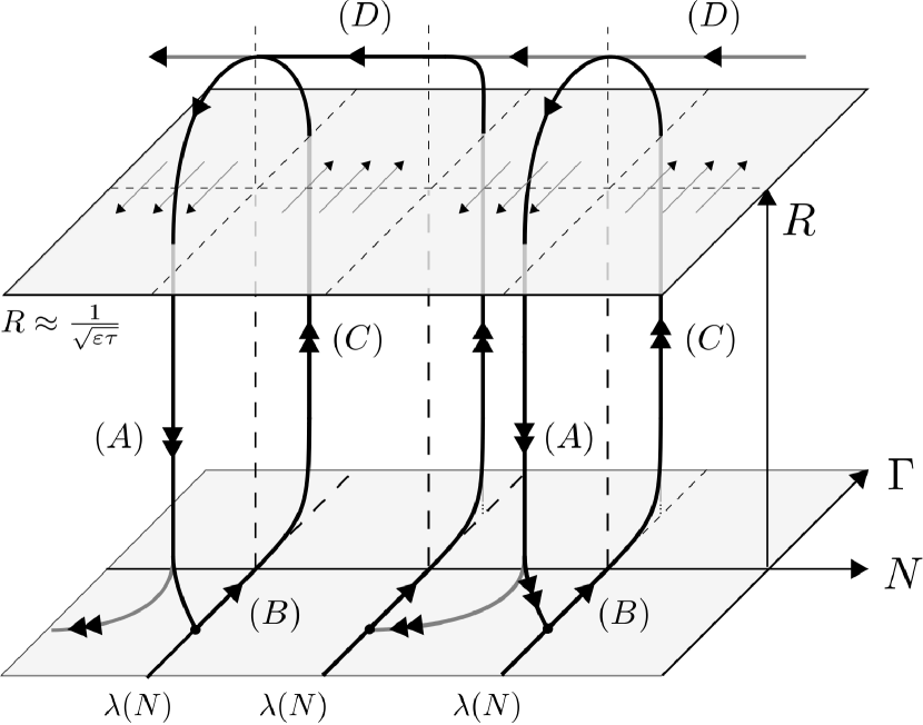
Figure 7: Slow-fast solution segments of averaged system (24)–(25) for $n^{\ast}(\tau)<N(t)<0$ (compare to segment (C) in Fig. 6). Fast segment (A): for $N(t)-1/\tau<\Gamma(t)<0$ ($N(t)$ is sufficiently small here) the solution is attracted fast by a branch $\lambda(N(t))$ of eigenvalues of $R(t)=0$. Slow segment (B): for $\Gamma(t)<0$ the solution stays close to $R(t)=0,~{}\lambda(N(t))$ and $N(t)$ slowly increases towards $N(t)=J>0$. Fast segment (C): for $\Gamma(t)>0$, $R(t)$ increases fast. Return flow (D): If $R(t)\geq 1/\sqrt{\varepsilon}$, $N(t)$ is strictly decreasing the parameters considered. If $\Gamma(t)$ is again negative, the solution is again attracted by a branch of eigenvalues (not necessarily the same). See Sec. III for details.

IV Discussion

In this manuscript, we numerically investigated the parameter regions, where LFFs and RPPs occur. We have shown that $\varepsilon\tau$ is an important quantity for the solution to exhibit LFFs. In fact, multiple time scale analysis suggests that $\varepsilon\tau<1/\eta$ is a necessary condition for LFFs to occur. In particular, we numerically observe that LFFs cease to exist for large time-delays $\tau>1/\varepsilon\eta$, if all other parameters are fixed. Additionally, we studied the spectrum of these solutions and conclude that LLFs are observed in the regime of weak chaos, at least for the considered parameter values. In the second part of the paper, we use a multi scale approach to characterize such solutions as bursting slow-fast oscillations. In particular, using singular geometric perturbation theory for delay differential equations, we have shown that within a dropout event the system can be reduced to a slow flow towards $N(t)=J$ along the zero solution $E(t)=0$ and that the amplitude builds up after the dropout is due to a weak instability for $n^{\ast}(\tau)<N(t)<0$ or strong instability for $N(t)>0$. Here $n^{\ast}(\tau)$ is the destabilization threshold for the off-state, which is explicitly computed. In order to describe the weakly chaotic solution for $E(t)>0$, we have imposed a finite-time averaging technique and investigated the corresponding system of ordinary differential equations. This approach can be considered as a generalization of reduced models that have already been applied in the analysis of the LK system Lenstra (1991); Huyet et al. (2000) and similar steps have been taken in the statistical theory of phase oscillators D’Huys, Jüngling, and Kinzel (2014). Our averaging method relies on the smallness of the parameters $\varepsilon$, $1/\tau$, and $\eta$, which are very natural for the LK system. Our analysis suggests that this method is applicable to a larger class of weakly chaotic solutions of singularly perturbed delay differential equations, where phenomena similar to LFFs exists. See Ref. Pieroux and Mandel, 2003 for an example in the context of the LK model.