The optimal multilinear Bohnenblust-Hille constants:
a computational solution for the real case

Abstract.

The Bohnenblust-Hille inequality for $m$-linear forms was proven in 1931 as a generalization of the famous 4/3-Littlewood inequality. The optimal constants (or at least their asymptotic behavior as $m$ grows) is unknown, but significant for applications. A recent result, obtained by Cavalcante, Teixeira and Pellegrino, provides a kind of algorithm, composed by finitely many elementary steps, giving as the final outcome the optimal truncated Bohnenblust-Hille constants of any order. But the procedure of Cavalcante et al. has a fairly large number of calculations and computer assistance cannot be avoided. In this paper we present a computational solution to the problem, using the Wolfram Language. We also use this approach to investigate a conjecture raised by Pellegrino and Teixeira, asserting that $C_{m}=2^{1-1/m}$ for all $m\in\mathbb{N}$ and to reveal interesting unknown facts about the geometry of $B_{\mathcal{L}(^{3}\mathbb{R}^{3})}$.

1. Introduction and notation

The Bohnenblust-Hille inequality was proven in 1931 (see [4]) by H. F. Bohnenblust (1906-2000) and C. E. Hille (1894-1980) as a generalization of the famous 4/3-Littlewood inequality. For the real case, it states that for each $m\in\mathbb{N}$ there exists an optimal constant $C_{m}\geq 1$ such that, for all $n\in\mathbb{N}$ and all $m$-linear forms $T:{\mathbb{R}^{n}\times\cdots\times\mathbb{R}^{n}\rightarrow\mathbb{R}}$, we have

(1) $$\biggl{(}\sum_{i_{1},...,i_{m}}^{n}|T(e_{i_{1}},...,e_{i_{m}})|^{\frac{2m}{m+1}}\biggr{)}^{\frac{m+1}{2m}}\leq C_{m}\sup\{|T(x_{1},...,x_{n})|\in\mathbb{R}:\|x_{i}\|\leq 1\}.$$

The numbers $C_{m}$, $m\in\mathbb{N}$, are called Bohnenblust-Hille constants. If we fix $n$ in the assumptions above, then we have the truncated Bohnenblust-Hille constants, denoted by $C_{m}^{(n)}$, which satisfy

(2) $$\biggl{(}\sum_{i_{1},...,i_{m}=1}^{n}|T(e_{i_{1}},...,e_{i_{m}})|^{\frac{2m}{m+1}}\biggr{)}^{\frac{m+1}{2m}}\leq C_{m}^{(n)}\sup\{|T(x_{1},...,x_{n})|\in\mathbb{R}:\|x_{i}\|\leq 1\}$$

for all $m$-linear forms $T:{\mathbb{R}^{n}\times\cdots\times\mathbb{R}^{n}\rightarrow\mathbb{R}}$. In this case, for each $m\in\mathbb{N}$, we have $C_{m}=\inf_{n}C_{m}^{(n)}$. For applications of the Bohnenblust-Hille inequality in physics we refer to [7] and references therein.

Let us establish some notations that will be carried out along this work. The transpose of a matrix $M$ will be denoted by $M^{t}$. For $k\in\mathbb{N}$, the $k$-th cartesian product of a set $A$ will be denoted by $A^{k}$. For example, $[\mathbb{R}^{n}]^{m}=\mathbb{R}^{n}\times\overset{m}{\cdots}\times\mathbb{R}^{n}$, $m,n\in\mathbb{N}$. If $E$ is a normed space, $B_{E}$ and $\text{ext}(B_{E})$ will denote the closed unit ball and the set of its extreme points, respectively. Given $m,n\in\mathbb{N}$, the $n$-dimensional Euclidean space $\mathbb{R}^{n}$ will be endowed with the norm

$$\|x\|=\sup\{\|x^{(i)}\|\in\mathbb{R}:i=1,...,n\},~{}\text{for all}~{}x=(x^{(1)},...,x^{(n)})\in\mathbb{R}^{n},$$

and the space ${\mathcal{L}(^{m}\mathbb{R}^{n})}$ of all $m$-linear forms $T:[\mathbb{R}^{n}]^{m}\rightarrow\mathbb{R}$ will be equipped with the norm

$$\|T\|=\sup\{|T(x_{1},...,x_{n})|\in\mathbb{R}:x_{i}\in\mathbb{R}^{n}~{}\text{and}~{}\|x_{i}\|\leq 1,i=1,...,n\},~{}\text{for all}~{}T\in{\mathcal{L}(^{m}\mathbb{R}^{n})}.$$

From the Krein-Milman theorem we obtain the formula

(3) $$\|T\|=\sup\{|T(x_{1},...,x_{n})|\in\mathbb{R}:x_{i}\in\text{ext}(B_{\mathbb{R}^{n}}),i=1,...,n\},~{}\text{for all}~{}T\in{\mathcal{L}(^{m}\mathbb{R}^{n})}.$$

For a complete discussion about extreme points of convex sets and the Krein-Milman (and Minkowski) theorem, we refer to [9, Chapter 8]. In the Example $8$ of the referenced chapter, we see that, for each $n\in\mathbb{N}$, the extreme points of the closed unit ball $B_{\mathbb{R}^{n}}$ in the $n$-dimensional Euclidean space $\mathbb{R}^{n}$ equipped with the sup norm is simply

(4) $$\text{ext}(B_{\mathbb{R}^{n}})=\{(\alpha_{1},...,\alpha_{n})\in\mathbb{R}^{n}:\alpha_{i}=1~{}\text{or}~{}\alpha_{i}=-1,~{}\text{for each}~{}i=1,...,n\}.$$

2. Bounds for the Bohnenblust-Hille constants

The Bohnenblust–Hille inequalities are part of a bigger family of inequalites called Hardy–Littlewood inequalities. Through the last years, researchers have chase for better upper bounds for the constants in these inequalities (for example [3], [2] and [8]). The better known approach, sometimes called interpolation (see [3] or [1] for an alternative approach via Hölder’s inequality), provides the following estimates (cf. [3, p.737, Corollary 3.4]):

$\begin{array}[]{|c|c|c|}\hline\cr m&\text{best known upper bound for }C_{m}&\\ \hline\cr 3&C_{3}\leq 1.6818&\\ \hline\cr 4&C_{4}\leq 1.8877&\\ \hline\cr 5&C_{5}\leq 2.0586&\\ \hline\cr 6&C_{6}\leq 2.2064&\\ \hline\cr 7&C_{7}\leq 2.3376&\\ \hline\cr 8&C_{8}\leq 2.4562&\\ \hline\cr\end{array}$

Table 1

This approach, however, doesn’t seem to be optimal, since it appears to lose information. For a discussion about this, we refer to [8]. On the other hand, the lower bounds $2^{1-1/m}$, $m\in\mathbb{N}$, obtained in 2014 (see [6]) were never improved. In [8], the authors propose a conjecture that these are in fact the optimal Bohnenblust-Hille constants (see p. 4). A new approach for the lower bounds, proposed in [5], is capable to provide the truncated Bohnenblust-Hille constants of any order (although the method is computationally costly). With this new method we are able to corroborate or refute this conjecture. In addition, it enables us to elaborate new ones. Through this paper we deal with this approach and its consequences and issues while we try to implement it computationally.

3. New approach to the constants

The new approach introduced in [5] for the truncated constants consists of finding the finite set $\text{ext}(B_{\mathcal{L}(^{m}\mathbb{R}^{n})})$ of the extreme points of the closed unit ball $B_{\mathcal{L}(^{m}\mathbb{R}^{n})}$ in the space ${\mathcal{L}(^{m}\mathbb{R}^{n})}$ of the $m$-linear forms $T:\mathbb{R}^{n}\times\overset{m}{\cdots}\times\mathbb{R}^{n}\to\mathbb{R}$. In fact, from (2), we have to solve the optimization problem

(5) $$C_{m}^{(n)}=\sup_{T\in B_{\mathcal{L}(^{m}\mathbb{R}^{n})}}\biggl{(}\sum_{i_{1},...,i_{m}}^{n}|T(e_{i_{1}},...,e_{i_{m}})|^{\frac{2m}{m+1}}\biggr{)}^{\frac{m+1}{2m}}.$$

From the Krein-Milman Theorem, the supremum (5) is attained in one of the extreme points of $B_{\mathcal{L}(^{m}\mathbb{R}^{n})}$, that is, we reduce the problem of finding the truncated Bohnenblust-Hille constants to the problem of calculating

(6) $$C_{m}^{(n)}=\max_{T\in\text{ext}(B_{\mathcal{L}(^{m}\mathbb{R}^{n})})}\biggl{(}\sum_{i_{1},...,i_{m}}^{n}|T(e_{i_{1}},...,e_{i_{m}})|^{\frac{2m}{m+1}}\biggr{)}^{\frac{m+1}{2m}}.$$

This way, it is sufficient to know the set $\text{ext}(B_{\mathcal{L}(^{m}\mathbb{R}^{n})})$ and, for this, we can apply the algorithm described in the next section.

4. A characterization for the extreme points of $B_{\mathcal{L}(^{m}\mathbb{R}^{n})}$

From the Theorem 15 of [5], we got a full characterization of the set $\text{ext}(B_{\mathcal{L}(^{m}\mathbb{R}^{n})})$ for all $m,n\in\mathbb{N}$. Now we will summarize the necessary definitions and state the theorem properly. More details and the proofs can be found within the reference [5].

Given $m,n\in\mathbb{N}$ and $x=(x_{1},...,x_{m})$, where $x_{i}\in\mathbb{R}^{n}$ for $i=1,...,m$, define $I_{n}\coloneqq\{1,...,n\}$ and, writing the elements of the cartesian $I_{n}^{m}$ in the form $\mathbf{j}=(j_{1},...,j_{m})$, put

$$x^{\mathbf{j}}\coloneqq x_{1}^{(j_{1})}\cdots x_{m}^{(j_{m})}$$

and

$$\omega(x)\coloneqq(x^{\mathbf{j}})_{\mathbf{j}\in I_{n}^{m}}\in\mathbb{R}^{n^{m}},$$

where the $n^{m}$-tuple $\omega(x)$ is ordered lexicographically. Also, let

(7) $$V_{n}^{m}\coloneqq\{\omega(x)\in\mathbb{R}^{n^{m}}:x\in[\text{ext}(B_{\mathbb{R}^{n}})]^{m}\}$$

and

(8) $$G_{n}^{m}\coloneqq\{\text{diag}(v):v\in V_{n}^{m}\},$$

where $\text{diag}(a_{i})_{i\in I_{k}}$, for $k\in\mathbb{N}$, denotes the $k\times k$ matrix obtained from a list $(a_{1},...,a_{k})$ putting it in the diagonal and filling the other entries with 0. Each $m$-linear form $T\in{\mathcal{L}(^{m}\mathbb{R}^{n})}$ can be represented uniquely in the form

(9) $$T(x)=\sum_{\mathbf{j}}a_{\mathbf{j}}x^{\mathbf{j}},~{}\text{for all}~{}x\in[\mathbb{R}^{n}]^{m},$$

for some unique real scalars $a_{\mathbf{j}}\in\mathbb{R}$, $\mathbf{j}\in I_{n}^{m}$. Letting $\mathfrak{m}^{T}\coloneqq(a_{\mathbf{j}})_{\mathbf{j}\in I_{n}^{m}}$, from (9) we have

(10) $$T(x)=\langle\mathfrak{m}^{T},\omega(x)\rangle,~{}\text{for all}~{}x\in[\mathbb{R}^{n}]^{m}.$$

It is easy to see that $\mathfrak{m}^{T\pm L}=\mathfrak{m}^{T}\pm\mathfrak{m}^{L}$ for all $T,L\in{\mathcal{L}(^{m}\mathbb{R}^{n})}$. Writing the formula (3) in the notation (10), we have

(11) $$\|T\|=\{|\langle\mathfrak{m}^{T},v\rangle|\in\mathbb{R}:v\in V_{n}^{m}\},~{}\text{for all}~{}T\in{\mathcal{L}(^{m}\mathbb{R}^{n})}.$$

So, from (11), we have

(12) $$B_{\mathcal{L}(^{m}\mathbb{R}^{n})}=\{T\in{\mathcal{L}(^{m}\mathbb{R}^{n})}:|\langle\mathfrak{m}^{T},v\rangle|\leq 1~{}\text{for all}~{}v\in V_{n}^{m}\}.$$

Now, fixing $m,n\in\mathbb{N}$, let us introduce the notations the will lead us to the characterization of $\text{ext}(B_{\mathcal{L}(^{m}\mathbb{R}^{n})})$. Denote by $\mathbf{1}$ the vector $(1,\overset{n^{m}}{...},1)$. We will refer to it as the fixed row. Let $\mathcal{B}$ be the set of all basis of $\mathbb{R}^{n^{m}}$ contained in $V_{n}^{m}$ and containing $\mathbf{1}$, say $\mathcal{=}\{\beta_{1},...,\beta_{s}\}$, for some $s\in\mathbb{N}$. Enumerate each $\beta_{j}$, $j\in I_{s}$, as $\beta_{j}=\{v_{j,1},...,v_{j,n^{m}}\}$ so that the “position” of $\mathbf{1}$ is the same for all $\beta_{j},j\in I_{s}$ (say the last one, that is, $v_{j,n^{m}}=\mathbf{1}$ for all $j\in I_{s}$). Define the matrices

$$H_{\beta_{j}}\coloneqq\left(\begin{array}[]{ccc}v_{j,1}^{(1)}&\cdots&v_{j,1}^{(n^{m})}\\ \vdots&\ddots&\vdots\\ v_{j,n^{m}}^{(1)}&\cdots&v_{j,n^{m}}^{(n^{m})}\end{array}\right),~{}\text{for all}~{}j\in I_{s},$$

and the set

$$\mathcal{A}\coloneqq\{\mathfrak{m}^{T}\in\mathbb{R}^{n^{m}}:H_{\beta_{j}}(\mathfrak{m}^{T})^{t}=e^{t},~{}\text{for some}~{}j\in I_{s}~{}\text{and}~{}e\in\text{ext}(B_{\mathbb{R}^{n^{m}}})\}.$$

The elements of $\mathcal{A}$ are precisely those of the form $\mathfrak{m}^{T}=(H_{\beta_{j}}^{-1}e^{t})^{t}$, where $e\in\text{ext}(B_{\mathbb{R}^{n^{m}}})$ and $j\in I_{s}$. Finally, define

(13) $$\mathcal{C}\coloneqq\{\mathfrak{m}^{T}\cdot g:\mathfrak{m}^{T}\in\mathcal{A},T\in B_{\mathcal{L}(^{m}\mathbb{R}^{n})}~{}\text{and}~{}g\in G_{n}^{m}\}.$$

From [5], Theorem 15, we conclude that

(14) $$\mathcal{C}=\text{ext}(B_{\mathcal{L}(^{m}\mathbb{R}^{n})}).$$

5. The algorithm

As we saw in the last section, we already have an algorithm to calculate the set $\text{ext}(B_{\mathcal{L}(^{m}\mathbb{R}^{n})})$, which one is composed by finitely many elementary steps. Before summarize the process, let us reduce the construction of the set $\mathcal{C}$ defined in (13).

Fix $m,n\in\mathbb{N}$. It is easy to verify that the sets $V_{n}^{m}$ defined in (7) and, consequently, $G_{n}^{m}$, defined in (8), are both symmetrical. Also, it is easy to see that matrices that are the same, up to symmetrical rows, leads to the same extreme points, up to symmetry. Further, since $-\mathbf{1}=(-1,\overset{m}{...},-1)\in G_{n}^{m}$, the last step adds all the missing symmetrical extreme points. So we don’t need to consider the complete set $\mathcal{B}$ of all the bases for $\mathbb{R}^{n^{m}}$ within $V_{n}^{m}$ and containing the fixed row $\mathbf{1}$. Instead, we remove from $V_{n}^{m}$ the symmetrical elements and consider a subset $\overline{V}_{n}^{m}$ that has the half of the size of $V_{n}^{m}$. Now, instead of $\mathcal{B}$, we take the subset $\mathcal{B}_{0}$ of the bases for $\mathbb{R}^{n^{m}}$ within $\overline{V}_{n}^{m}$ and containing the fixed row. This reduction has an enormous impact in the number of matrices considered in the process. For example, for the planar case (that is, when $n=2$), this reduction leads to a single base $\beta\in\mathcal{B}_{0}$, that is, the process will be made with just one matrix. Other reduction in the process concerns the set $\text{ext}(B_{\mathbb{R}^{n^{m}}})$ while calculating $\mathcal{A}$: we only need to proceed with the half of it. The argument is analogously by symmetry and the fact that $-\mathbf{1}\in G_{n}^{m}$, what leads to a subset $\mathcal{A}_{0}$ with the half of the size.

Now we are able to describe the process that leads to the set $\mathcal{C}$ defined in (13). Let $m,n\in\mathbb{N}$. The constructive process consists of performing each of the steps below:

1. Calculate $I_{n}^{m}$, $[\text{ext}(B_{\mathbb{R}^{n}})]^{m}$ and $\omega(x)$ for all $x\in[\text{ext}(B_{\mathbb{R}^{n}})]^{m}$ and obtain the set $V_{n}^{m}$;

2. Obtain the set $\overline{V}_{n}^{m}$ from $V_{n}^{m}$ by removing its symmetrical elements;

3. Consider the set $\mathcal{M}$ of all the invertible matrices with lines in $\overline{V}_{n}^{m}$, with the fixed row 1 as the last line and removing those that are the same under row switching;

4. For the half of elements from $e\in\text{ext}(B_{\mathbb{R}^{n^{m}}})$ (disregarding the symmetric ones) and for each matrix obtained from the last step, calculate $mf^{T}=e(H_{\beta}^{-1})^{t}$, what gives us the set $\mathcal{A}_{0}$;

5. Calculate $\mathcal{C}_{0}=\mathcal{A}_{0}\cap B_{\mathcal{L}(^{m}\mathbb{R}^{n})}$ using (12);

6. Finally, obtain $\mathcal{C}$ as the collection of the $n^{m}$-tuples of the form $\mathfrak{m}^{T}\cdot g$, with $\mathfrak{m}^{T}\in\mathcal{C}_{0}$ and $g\in G_{n}^{m}$. From (14), this set is $\text{ext}(B_{\mathcal{L}(^{m}\mathbb{R}^{n})})$.

6. Computational implementation

The process described step-by-step in the last section was implemented by us in Wolfram Language using the software Mathematica. Two codes were built. The first one takes as inicial inputs the values of $m$ and $n$ and execute all the steps listed before in the very same way it was described. We will refer to this one as the full program. The second code, on the other hand, aims to find extreme points in cases where we can’t execute the full program due to computational limitations. This one, which will be referred as the random program, takes as initial inputs the values of $m$, $n$ and three other ones: (1) the minimum quantity of monomials that the extreme points to be found should have; (2) the quantity of randomly generated points within $\text{ext}(B_{\mathbb{R}^{n^{m}}})$ per test; and (3) the number of times each matrix randomly generated will be tested. Given these inputs, the random program execute the following steps:

1. Execute steps 1 and 2 of the full program;

2. Take a random sample $\{v_{1},...,v_{n^{m}-1}\}$ of $n^{m}-1$ elements from $\overline{V}_{n}^{m}\backslash{\textbf{1}}$, consider the matrix $H$ whose rows are the vectors from $\{v_{1},...,v_{n^{m}-1},\textbf{1}\}$ and calculate its determinant in order to verify if it is invertible;

3. If $H$ is invertible, proceed to the next step, if not, generate another random sample and repeat until the matrix $H$ obtained is invertible;

4. Generate randomly a set of points from $\text{ext}(B_{\mathbb{R}^{n^{m}}})$ (the quantity decided in the inicial input), calculate $T_{e,H}=(H^{-1}e^{t})^{t}$ with them and collect (using 12) those that belongs to $B_{\mathcal{L}(^{m}\mathbb{R}^{n})}$;

5. If the set collected in the last step is empty, generate new randomly points from $\text{ext}(B_{\mathbb{R}^{n^{m}}})$ and repeat until some form $T_{e,H}$ within $B_{\mathcal{L}(^{m}\mathbb{R}^{n})}$ is found;

6. Within the forms found in the last step, collect those whose quantity of monomials match the minimum required in the inicial input and count this as one test with this matrix;

7. Repeat again the steps from 4 forward the number of times decided in the inicial output;

8. If there is some remaining point (what will be extreme points with a interesting quantity of monomials), the algorithm ends, if not, generate another matrix and repeat until something is found.

The Mathematica notebook files (.nd) containing these two codes can be found in the link https://goo.gl/MsdyUV. One observation is that both the notebooks have, at the end, a piece of code aiming to evaluate the Bohnenblust-Hille constants based in the results obtained with the programs above. With the full program, the result is the exact truncated Bohnenblust-Hille constant, while with the random program, the result is a lower bound. More about this piece of code and the geral output of the programs will be discussed later in this paper.

7. About the conjecture

Fixing $m\in\mathbb{N}$, as we already discussed, the better known lower bounds for the Bohnen-blust-Hille constants $C_{m}$ are $2^{1-1/m}$. The discussion and conjecture that these are the optimal ones first appeared at [8]. There, the authors proved that it is necessary forms with $4^{m-1}$ monomials, at least, in order to overcome this value. They key seems to have forms with many monomials and little norm. For example, for $m=3$, we need forms with more than 16 monomials to overcome the better known lower bound $2^{1-1/3}$. If this is not the optimal constant, that is, if $2^{1-1/3}<C_{m}=\sup\{C_{3}^{(n)}:n\in\mathbb{N}\}$, certainly there exists one point in $\text{ext}(B_{\mathcal{L}(^{3}\mathbb{R}^{n})})$, for some $n\in\mathbb{N}$, with more than 16 monomials. However, the existence of these points remain unknown. On the other hand, if there are no extreme points in $\text{ext}(B_{\mathcal{L}(^{3}\mathbb{R}^{n})}$, for all $n\in\mathbb{N}$, with more than $16$ monimials, then the conjecture is confirmed and the optimal Bohnenblust-Hille constant is $2^{1-1/3}$. Obviously this discussion applies to any value of $m\in\mathbb{N}$ rather than $m=3$.

There are some possibilities with the approach we aim to apply. The first one and more hopeful is to corroborate the conjecture, what can happens in many ways. For example: (1) there are no extreme points with more than $4^{m-1}$ monomials; or (2) even if there are some, they don’t overcome the conjectured value. Other possibility with this approach is to find an extreme point that attain a known upper bound, what is sufficient to find the optimal constant for the case of $m$.

Speaking about the possibilities with our codes, they allow us to: (1) put the approach in practice; (2) find extreme points for $B_{\mathcal{L}(^{m}\mathbb{R}^{n})}$ in cases where they were never found; (3) analyse the behavior of the extreme points in association with the Bohnenblust-Hille inequality; and (4) investigate the existence of extreme points in $B_{\mathcal{L}(^{m}\mathbb{R}^{n})}$ with more than $4^{m-1}$ monomials.

8. Investigating the Bohnenblust-Hille constants

This section aims to describe the last piece of code included in both full and random programs. Given $m,n\in\mathbb{N}$, the aim of the code is to calculate the value of the convex function $f:B_{\mathcal{L}(^{m}\mathbb{R}^{n})}\to\mathbb{R}$ given by

(15) $$f(T)=\biggl{(}\sum_{i_{1},...,i_{m}=1}^{n}|T(e_{i_{1}},...,e_{i_{m}})|^{\frac{2m}{m+1}}\biggr{)}^{\frac{m+1}{2m}}$$

with the extreme points $T$ found within $B_{\mathcal{L}(^{m}\mathbb{R}^{n})}$ and then take the maximum value. With the full program, this process leads to the truncated constant (6), and with the random program, it leads to a lower bound for it and, consequently, for the optimal constant $m\in\mathbb{N}$.

As we already mentioned, this last piece of code was included at the end of both programs. The general outputs are:

1. The maximum value obtained, say $M\in\mathbb{R}$;

2. Evaluation (true-false) of the the sentence $M\leq 2^{1-1/m}$;

3. The quantity of extreme points found;

4. The list of extreme points in matricial form;

5. the list of calculations (15) made with each extreme points found (exhibited in the respective order in relation to Out 4).

If Out 2 returns False, this means that we refute the conjecture. Searching in Out 5 the user can find the extreme point that leads the maximum result, pick its position and look at the extreme point in Out 4 at the same position. This is the interesting form found though the program. We can also easily count the number of monomials in each extreme point found and see if something interesting appear.

9. Some results and new conjectures

Since, for each $m\in\mathbb{N}$, we are looking for extreme points with more than $4^{m-1}$ monomials and in ${\mathcal{L}(^{m}\mathbb{R}^{n})}$ the forms have $n^{m}$ at maximum, it is interesting to fix $m$ and take $n$ such that $n^{m}>4^{m-1}$, that is, $n>\sqrt[m]{4^{m-1}}$. Since we aim to investigate the Bohnenblust-Hille constants and since for $m=2$ we recover the 4/3-Littlewood inequality, for which we already know that $C_{m}=\sqrt{2}$, it is interesting for us to run the case $m\geq 3$. So the smallest interesting cases are $n\geq 3$.

With the computational resources available for us, we couldn’t run the full program for $m\geq 3$ and $n\geq 3$ (although for smaller values of $m$ or $n$ it was possible). The issues are discussed in the last section of this paper. We could, however, adjust the random program to fit our available resources and find some interesting results.

Configuring the random program to test each matrix 50 times and generate 10000 points from $\text{ext}(B_{\mathbb{R}^{3^{3}}})$ per evaluation, we could find some interesting points. While searching for extreme with at least 16 monomials, the program find a lot of them easily. For example, the form

$$T_{16}=\frac{1}{4}(-1,-1,0,-1,-1,0,0,0,0,-1,0,-1,0,1,1,-1,1,0,0,-1,1,1,0,-1,-1,1,0)$$

is one of the extreme points found. All of them attained the conjectured ($2^{1-1/3}\approx 1.5874$) value when we calculated (15). Although doubting the existence of extreme points in $B_{\mathcal{L}(^{3}\mathbb{R}^{3})}$ with more than 16 monomials, we ran the code searching extremes with at least 17 monomials. After about 6 hours, for our surprise, there were found two points. The first, with 19 monomials, is

$$T_{19}=-\frac{1}{8}(1,2,-1,0,0,0,-1,2,-1,1,1,4,1,0,-1,0,1,-3,0,1,1,-1,0,1,1,1,0).$$

The second, with 20 monomials, is

$$T_{20}=-\frac{1}{8}(1,0,-1,0,0,0,1,0,-1,1,-1,-2,1,2,1,0,1,1,2,1,-1,3,-2,3,-1,-1,0).$$

Another interesting fact about this discovery, rather than the existence, was the values of (15) for these two monomials. We got

$$f(T_{19})\approx 1.30810~{}~{}\text{e}~{}~{}f(T_{20})\approx 1.35541.$$

That is, $f(T_{19})<f(T_{20})<f(T_{16})$. The “good” matrix that generated these points is

$$\left(\begin{array}[]{rrrrrrrrrrrrrrrrrrrrrrrrrrr}\!\!1\!\!&\!\!1\!\!&\!\!1\!\!&\!\!1\!\!&\!\!1\!\!&\!\!1\!\!&\!\!1\!\!&\!\!1\!\!&\!\!1\!\!&\!\!1\!\!&\!\!1\!\!&\!\!1\!\!&\!\!1\!\!&\!\!1\!\!&\!\!1\!\!&\!\!1\!\!&\!\!1\!\!&\!\!1\!\!&\!\!1\!\!&\!\!1\!\!&\!\!1\!\!&\!\!1\!\!&\!\!1\!\!&\!\!1\!\!&\!\!1\!\!&\!\!1\!\!&\!\!1\\ \!\!1\!\!&\!\!-1\!\!&\!\!-1\!\!&\!\!-1\!\!&\!\!1\!\!&\!\!1\!\!&\!\!-1\!\!&\!\!1\!\!&\!\!1\!\!&\!\!1\!\!&\!\!-1\!\!&\!\!-1\!\!&\!\!-1\!\!&\!\!1\!\!&\!\!1\!\!&\!\!-1\!\!&\!\!1\!\!&\!\!1\!\!&\!\!1\!\!&\!\!-1\!\!&\!\!-1\!\!&\!\!-1\!\!&\!\!1\!\!&\!\!1\!\!&\!\!-1\!\!&\!\!1\!\!&\!\!1\\ \!\!1\!\!&\!\!1\!\!&\!\!-1\!\!&\!\!-1\!\!&\!\!-1\!\!&\!\!1\!\!&\!\!-1\!\!&\!\!-1\!\!&\!\!1\!\!&\!\!-1\!\!&\!\!-1\!\!&\!\!1\!\!&\!\!1\!\!&\!\!1\!\!&\!\!-1\!\!&\!\!1\!\!&\!\!1\!\!&\!\!-1\!\!&\!\!1\!\!&\!\!1\!\!&\!\!-1\!\!&\!\!-1\!\!&\!\!-1\!\!&\!\!1\!\!&\!\!-1\!\!&\!\!-1\!\!&\!\!1\\ \!\!1\!\!&\!\!-1\!\!&\!\!1\!\!&\!\!-1\!\!&\!\!1\!\!&\!\!-1\!\!&\!\!1\!\!&\!\!-1\!\!&\!\!1\!\!&\!\!-1\!\!&\!\!1\!\!&\!\!-1\!\!&\!\!1\!\!&\!\!-1\!\!&\!\!1\!\!&\!\!-1\!\!&\!\!1\!\!&\!\!-1\!\!&\!\!-1\!\!&\!\!1\!\!&\!\!-1\!\!&\!\!1\!\!&\!\!-1\!\!&\!\!1\!\!&\!\!-1\!\!&\!\!1\!\!&\!\!-1\\ \!\!1\!\!&\!\!1\!\!&\!\!1\!\!&\!\!1\!\!&\!\!1\!\!&\!\!1\!\!&\!\!-1\!\!&\!\!-1\!\!&\!\!-1\!\!&\!\!-1\!\!&\!\!-1\!\!&\!\!-1\!\!&\!\!-1\!\!&\!\!-1\!\!&\!\!-1\!\!&\!\!1\!\!&\!\!1\!\!&\!\!1\!\!&\!\!1\!\!&\!\!1\!\!&\!\!1\!\!&\!\!1\!\!&\!\!1\!\!&\!\!1\!\!&\!\!-1\!\!&\!\!-1\!\!&\!\!-1\\ \!\!1\!\!&\!\!-1\!\!&\!\!1\!\!&\!\!-1\!\!&\!\!1\!\!&\!\!-1\!\!&\!\!-1\!\!&\!\!1\!\!&\!\!-1\!\!&\!\!-1\!\!&\!\!1\!\!&\!\!-1\!\!&\!\!1\!\!&\!\!-1\!\!&\!\!1\!\!&\!\!1\!\!&\!\!-1\!\!&\!\!1\!\!&\!\!-1\!\!&\!\!1\!\!&\!\!-1\!\!&\!\!1\!\!&\!\!-1\!\!&\!\!1\!\!&\!\!1\!\!&\!\!-1\!\!&\!\!1\\ \!\!1\!\!&\!\!-1\!\!&\!\!1\!\!&\!\!-1\!\!&\!\!1\!\!&\!\!-1\!\!&\!\!1\!\!&\!\!-1\!\!&\!\!1\!\!&\!\!-1\!\!&\!\!1\!\!&\!\!-1\!\!&\!\!1\!\!&\!\!-1\!\!&\!\!1\!\!&\!\!-1\!\!&\!\!1\!\!&\!\!-1\!\!&\!\!1\!\!&\!\!-1\!\!&\!\!1\!\!&\!\!-1\!\!&\!\!1\!\!&\!\!-1\!\!&\!\!1\!\!&\!\!-1\!\!&\!\!1\\ \!\!1\!\!&\!\!-1\!\!&\!\!1\!\!&\!\!-1\!\!&\!\!1\!\!&\!\!-1\!\!&\!\!-1\!\!&\!\!1\!\!&\!\!-1\!\!&\!\!-1\!\!&\!\!1\!\!&\!\!-1\!\!&\!\!1\!\!&\!\!-1\!\!&\!\!1\!\!&\!\!1\!\!&\!\!-1\!\!&\!\!1\!\!&\!\!1\!\!&\!\!-1\!\!&\!\!1\!\!&\!\!-1\!\!&\!\!1\!\!&\!\!-1\!\!&\!\!-1\!\!&\!\!1\!\!&\!\!-1\\ \!\!1\!\!&\!\!1\!\!&\!\!-1\!\!&\!\!-1\!\!&\!\!-1\!\!&\!\!1\!\!&\!\!-1\!\!&\!\!-1\!\!&\!\!1\!\!&\!\!-1\!\!&\!\!-1\!\!&\!\!1\!\!&\!\!1\!\!&\!\!1\!\!&\!\!-1\!\!&\!\!1\!\!&\!\!1\!\!&\!\!-1\!\!&\!\!-1\!\!&\!\!-1\!\!&\!\!1\!\!&\!\!1\!\!&\!\!1\!\!&\!\!-1\!\!&\!\!1\!\!&\!\!1\!\!&\!\!-1\\ \!\!1\!\!&\!\!-1\!\!&\!\!1\!\!&\!\!1\!\!&\!\!-1\!\!&\!\!1\!\!&\!\!-1\!\!&\!\!1\!\!&\!\!-1\!\!&\!\!-1\!\!&\!\!1\!\!&\!\!-1\!\!&\!\!-1\!\!&\!\!1\!\!&\!\!-1\!\!&\!\!1\!\!&\!\!-1\!\!&\!\!1\!\!&\!\!-1\!\!&\!\!1\!\!&\!\!-1\!\!&\!\!-1\!\!&\!\!1\!\!&\!\!-1\!\!&\!\!1\!\!&\!\!-1\!\!&\!\!1\\ \!\!1\!\!&\!\!1\!\!&\!\!1\!\!&\!\!-1\!\!&\!\!-1\!\!&\!\!-1\!\!&\!\!-1\!\!&\!\!-1\!\!&\!\!-1\!\!&\!\!1\!\!&\!\!1\!\!&\!\!1\!\!&\!\!-1\!\!&\!\!-1\!\!&\!\!-1\!\!&\!\!-1\!\!&\!\!-1\!\!&\!\!-1\!\!&\!\!1\!\!&\!\!1\!\!&\!\!1\!\!&\!\!-1\!\!&\!\!-1\!\!&\!\!-1\!\!&\!\!-1\!\!&\!\!-1\!\!&\!\!-1\\ \!\!1\!\!&\!\!-1\!\!&\!\!-1\!\!&\!\!-1\!\!&\!\!1\!\!&\!\!1\!\!&\!\!-1\!\!&\!\!1\!\!&\!\!1\!\!&\!\!1\!\!&\!\!-1\!\!&\!\!-1\!\!&\!\!-1\!\!&\!\!1\!\!&\!\!1\!\!&\!\!-1\!\!&\!\!1\!\!&\!\!1\!\!&\!\!-1\!\!&\!\!1\!\!&\!\!1\!\!&\!\!1\!\!&\!\!-1\!\!&\!\!-1\!\!&\!\!1\!\!&\!\!-1\!\!&\!\!-1\\ \!\!1\!\!&\!\!1\!\!&\!\!1\!\!&\!\!1\!\!&\!\!1\!\!&\!\!1\!\!&\!\!-1\!\!&\!\!-1\!\!&\!\!-1\!\!&\!\!-1\!\!&\!\!-1\!\!&\!\!-1\!\!&\!\!-1\!\!&\!\!-1\!\!&\!\!-1\!\!&\!\!1\!\!&\!\!1\!\!&\!\!1\!\!&\!\!-1\!\!&\!\!-1\!\!&\!\!-1\!\!&\!\!-1\!\!&\!\!-1\!\!&\!\!-1\!\!&\!\!1\!\!&\!\!1\!\!&\!\!1\\ \!\!1\!\!&\!\!1\!\!&\!\!-1\!\!&\!\!1\!\!&\!\!1\!\!&\!\!-1\!\!&\!\!-1\!\!&\!\!-1\!\!&\!\!1\!\!&\!\!1\!\!&\!\!1\!\!&\!\!-1\!\!&\!\!1\!\!&\!\!1\!\!&\!\!-1\!\!&\!\!-1\!\!&\!\!-1\!\!&\!\!1\!\!&\!\!1\!\!&\!\!1\!\!&\!\!-1\!\!&\!\!1\!\!&\!\!1\!\!&\!\!-1\!\!&\!\!-1\!\!&\!\!-1\!\!&\!\!1\\ \!\!1\!\!&\!\!-1\!\!&\!\!-1\!\!&\!\!1\!\!&\!\!-1\!\!&\!\!-1\!\!&\!\!1\!\!&\!\!-1\!\!&\!\!-1\!\!&\!\!-1\!\!&\!\!1\!\!&\!\!1\!\!&\!\!-1\!\!&\!\!1\!\!&\!\!1\!\!&\!\!-1\!\!&\!\!1\!\!&\!\!1\!\!&\!\!1\!\!&\!\!-1\!\!&\!\!-1\!\!&\!\!1\!\!&\!\!-1\!\!&\!\!-1\!\!&\!\!1\!\!&\!\!-1\!\!&\!\!-1\\ \!\!1\!\!&\!\!-1\!\!&\!\!1\!\!&\!\!-1\!\!&\!\!1\!\!&\!\!-1\!\!&\!\!1\!\!&\!\!-1\!\!&\!\!1\!\!&\!\!1\!\!&\!\!-1\!\!&\!\!1\!\!&\!\!-1\!\!&\!\!1\!\!&\!\!-1\!\!&\!\!1\!\!&\!\!-1\!\!&\!\!1\!\!&\!\!1\!\!&\!\!-1\!\!&\!\!1\!\!&\!\!-1\!\!&\!\!1\!\!&\!\!-1\!\!&\!\!1\!\!&\!\!-1\!\!&\!\!1\\ \!\!1\!\!&\!\!1\!\!&\!\!-1\!\!&\!\!1\!\!&\!\!1\!\!&\!\!-1\!\!&\!\!1\!\!&\!\!1\!\!&\!\!-1\!\!&\!\!1\!\!&\!\!1\!\!&\!\!-1\!\!&\!\!1\!\!&\!\!1\!\!&\!\!-1\!\!&\!\!1\!\!&\!\!1\!\!&\!\!-1\!\!&\!\!-1\!\!&\!\!-1\!\!&\!\!1\!\!&\!\!-1\!\!&\!\!-1\!\!&\!\!1\!\!&\!\!-1\!\!&\!\!-1\!\!&\!\!1\\ \!\!1\!\!&\!\!1\!\!&\!\!-1\!\!&\!\!1\!\!&\!\!1\!\!&\!\!-1\!\!&\!\!1\!\!&\!\!1\!\!&\!\!-1\!\!&\!\!1\!\!&\!\!1\!\!&\!\!-1\!\!&\!\!1\!\!&\!\!1\!\!&\!\!-1\!\!&\!\!1\!\!&\!\!1\!\!&\!\!-1\!\!&\!\!1\!\!&\!\!1\!\!&\!\!-1\!\!&\!\!1\!\!&\!\!1\!\!&\!\!-1\!\!&\!\!1\!\!&\!\!1\!\!&\!\!-1\\ \!\!1\!\!&\!\!-1\!\!&\!\!1\!\!&\!\!1\!\!&\!\!-1\!\!&\!\!1\!\!&\!\!-1\!\!&\!\!1\!\!&\!\!-1\!\!&\!\!-1\!\!&\!\!1\!\!&\!\!-1\!\!&\!\!-1\!\!&\!\!1\!\!&\!\!-1\!\!&\!\!1\!\!&\!\!-1\!\!&\!\!1\!\!&\!\!1\!\!&\!\!-1\!\!&\!\!1\!\!&\!\!1\!\!&\!\!-1\!\!&\!\!1\!\!&\!\!-1\!\!&\!\!1\!\!&\!\!-1\\ \!\!1\!\!&\!\!-1\!\!&\!\!-1\!\!&\!\!1\!\!&\!\!-1\!\!&\!\!-1\!\!&\!\!1\!\!&\!\!-1\!\!&\!\!-1\!\!&\!\!1\!\!&\!\!-1\!\!&\!\!-1\!\!&\!\!1\!\!&\!\!-1\!\!&\!\!-1\!\!&\!\!1\!\!&\!\!-1\!\!&\!\!-1\!\!&\!\!1\!\!&\!\!-1\!\!&\!\!-1\!\!&\!\!1\!\!&\!\!-1\!\!&\!\!-1\!\!&\!\!1\!\!&\!\!-1\!\!&\!\!-1\\ \!\!1\!\!&\!\!-1\!\!&\!\!1\!\!&\!\!1\!\!&\!\!-1\!\!&\!\!1\!\!&\!\!-1\!\!&\!\!1\!\!&\!\!-1\!\!&\!\!1\!\!&\!\!-1\!\!&\!\!1\!\!&\!\!1\!\!&\!\!-1\!\!&\!\!1\!\!&\!\!-1\!\!&\!\!1\!\!&\!\!-1\!\!&\!\!-1\!\!&\!\!1\!\!&\!\!-1\!\!&\!\!-1\!\!&\!\!1\!\!&\!\!-1\!\!&\!\!1\!\!&\!\!-1\!\!&\!\!1\\ \!\!1\!\!&\!\!1\!\!&\!\!-1\!\!&\!\!-1\!\!&\!\!-1\!\!&\!\!1\!\!&\!\!1\!\!&\!\!1\!\!&\!\!-1\!\!&\!\!-1\!\!&\!\!-1\!\!&\!\!1\!\!&\!\!1\!\!&\!\!1\!\!&\!\!-1\!\!&\!\!-1\!\!&\!\!-1\!\!&\!\!1\!\!&\!\!1\!\!&\!\!1\!\!&\!\!-1\!\!&\!\!-1\!\!&\!\!-1\!\!&\!\!1\!\!&\!\!1\!\!&\!\!1\!\!&\!\!-1\\ \!\!1\!\!&\!\!-1\!\!&\!\!-1\!\!&\!\!-1\!\!&\!\!1\!\!&\!\!1\!\!&\!\!1\!\!&\!\!-1\!\!&\!\!-1\!\!&\!\!1\!\!&\!\!-1\!\!&\!\!-1\!\!&\!\!-1\!\!&\!\!1\!\!&\!\!1\!\!&\!\!1\!\!&\!\!-1\!\!&\!\!-1\!\!&\!\!-1\!\!&\!\!1\!\!&\!\!1\!\!&\!\!1\!\!&\!\!-1\!\!&\!\!-1\!\!&\!\!-1\!\!&\!\!1\!\!&\!\!1\\ \!\!1\!\!&\!\!1\!\!&\!\!-1\!\!&\!\!1\!\!&\!\!1\!\!&\!\!-1\!\!&\!\!-1\!\!&\!\!-1\!\!&\!\!1\!\!&\!\!-1\!\!&\!\!-1\!\!&\!\!1\!\!&\!\!-1\!\!&\!\!-1\!\!&\!\!1\!\!&\!\!1\!\!&\!\!1\!\!&\!\!-1\!\!&\!\!-1\!\!&\!\!-1\!\!&\!\!1\!\!&\!\!-1\!\!&\!\!-1\!\!&\!\!1\!\!&\!\!1\!\!&\!\!1\!\!&\!\!-1\\ \!\!1\!\!&\!\!1\!\!&\!\!1\!\!&\!\!1\!\!&\!\!1\!\!&\!\!1\!\!&\!\!-1\!\!&\!\!-1\!\!&\!\!-1\!\!&\!\!1\!\!&\!\!1\!\!&\!\!1\!\!&\!\!1\!\!&\!\!1\!\!&\!\!1\!\!&\!\!-1\!\!&\!\!-1\!\!&\!\!-1\!\!&\!\!-1\!\!&\!\!-1\!\!&\!\!-1\!\!&\!\!-1\!\!&\!\!-1\!\!&\!\!-1\!\!&\!\!1\!\!&\!\!1\!\!&\!\!1\\ \!\!1\!\!&\!\!-1\!\!&\!\!-1\!\!&\!\!-1\!\!&\!\!1\!\!&\!\!1\!\!&\!\!-1\!\!&\!\!1\!\!&\!\!1\!\!&\!\!-1\!\!&\!\!1\!\!&\!\!1\!\!&\!\!1\!\!&\!\!-1\!\!&\!\!-1\!\!&\!\!1\!\!&\!\!-1\!\!&\!\!-1\!\!&\!\!1\!\!&\!\!-1\!\!&\!\!-1\!\!&\!\!-1\!\!&\!\!1\!\!&\!\!1\!\!&\!\!-1\!\!&\!\!1\!\!&\!\!1\\ \!\!1\!\!&\!\!1\!\!&\!\!1\!\!&\!\!1\!\!&\!\!1\!\!&\!\!1\!\!&\!\!1\!\!&\!\!1\!\!&\!\!1\!\!&\!\!-1\!\!&\!\!-1\!\!&\!\!-1\!\!&\!\!-1\!\!&\!\!-1\!\!&\!\!-1\!\!&\!\!-1\!\!&\!\!-1\!\!&\!\!-1\!\!&\!\!-1\!\!&\!\!-1\!\!&\!\!-1\!\!&\!\!-1\!\!&\!\!-1\!\!&\!\!-1\!\!&\!\!-1\!\!&\!\!-1\!\!&\!\!-1\\ &&&&&&&&&&&&&&&&&&&&&&&&&&\end{array}\right).$$

Believing that this matrix would lead to more interesting results, we ran a modified version of the full program to calculate all the extreme points that this matrix generate. There were found 55720 nontrivial (that is, different than the canonical vectors) extreme points: 2376 with 4 monomials, 3456 with 8 monomials, 18144 with 10 monomials, 20736 with 13 monomials, 6912 with 16 monomials, 768 with 19 monomials, 1536 with 20 monomials, 256 with 21 monomials and 1536 with 22 monomials. Some example are:

$$T_{4}=\frac{1}{2}(1,1,0,0,0,0,0,0,0,0,0,0,0,0,0,-1,1,0,0,0,0,0,0,0,0,0,0),$$

$$T_{8}=\frac{1}{4}(3,0,1,-1,0,1,0,0,0,0,0,0,0,0,0,0,0,0,1,0,-1,1,0,-1,0,0,0)$$

$$T_{10}=\frac{1}{4}(-2,-2,0,0,0,0,0,0,0,0,0,0,1,-1,0,-1,1,0,0,0,0,-1,1,0,-1,1,0)$$

$$T_{13}=\frac{1}{4}(2,1,1,1,0,-1,-1,1,0,0,0,0,0,0,0,0,0,0,0,1,-1,-1,0,1,-1,1,0)$$

$$T_{16}=\frac{1}{4}(-1,-1,0,0,-1,1,1,0,1,1,1,0,-1,0,1,0,1,1,0,0,0,-1,1,0,1,-1,0)$$

$$T_{21}=\frac{1}{8}(1,0,1,0,2,2,1,-2,-1,1,1,0,-1,0,-1,0,1,-1,0,-1,1,1,-2,-1,1,1,-4)~{}~{}\text{e}$$

$$T_{22}=\frac{1}{8}(-3,0,-1,0,2,-2,1,2,1,1,1,0,1,0,-1,0,1,1,2,-1,1,-1,2,-1,-1,1,2).$$

With them, we obtained the following results:

$$f(T_{4})\approx 1.25992,~{}~{}f(T_{8})\approx 1.32461,~{}~{}f(T_{10})\approx 1.42837,~{}~{}f(T_{13})\approx 1.50893,$$

$$f(T_{16})\approx 1.5874,~{}~{}f(T_{21})\approx 1.34546~{}~{}\text{e}~{}~{}f(T_{22})\approx 1.39213.$$

Our discoveries are resumed in the Figure 1.

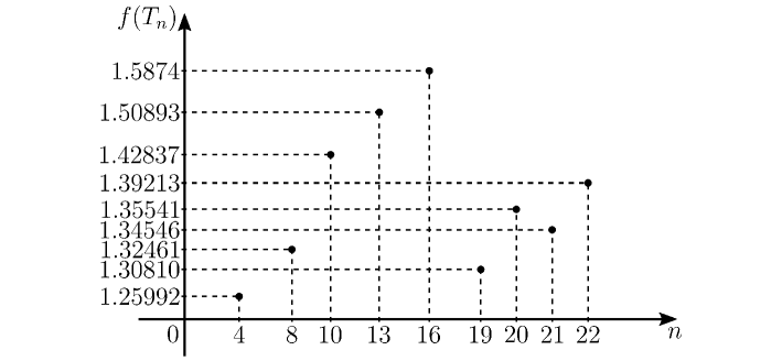
Figure 1. Graph of $n\mapsto f(T_{n})$.

As we saw above, we couldn’t refute the conjecture arisen in [8], but corroborate it. Moreover, some interesting facts that we found can suggest new conjectures. As we can see in the Figure 1, the extreme points with 16 monomials are “special” in the sense that the value of (15) were bigger with them than with any other extreme points, even those with more monomials. So there are in fact extreme points that have more than 16 monomials for the case $m=n=3$. An interesting thing that we can notice, however, is that the extreme that led to the best value of (15) have the same coefficient in every monomial. They are, in essence, the same kind of form found in [6], that is, with coefficient $1$ or $-1$ in each parcel. This way, fixing $m,n\in\mathbb{N}$, two ideas come in mind: (1) maybe the extreme points of $B_{\mathcal{L}(^{m}\mathbb{R}^{n})}$ with more than $4^{m-1}$ monomials don’t have the same coefficient for each of its monomials; and (2) maybe forms whose monomials don’t have the same coefficient can’t attain the best known lower bound $2^{1-1/m}$. These two open problems could be conceived as conjectures. If they were proved, then we would conclude that the conjecture arisen in [8] is true, that is, $C_{m}=2^{1-1/m}$.

10. The issues and future perspectives

In this last section we discuss some issues with the actual code and the reason why we couldn’t run the programs for larger values.

There are two big sets that are dealt with in the process described in the Section 5. The first one is $\text{ext}(B_{\mathbb{R}^{n^{m}}})$, $m,n\in\mathbb{N}$. For large values of $n$ and $m$, this set is too big for any computer to hold. However, as we saw in (4) and using the function IntegerDigits from the Wolfram Language (see the code attached), we have a simple solution to calculate this set one-element-by-one without holding it entirely at once. This way, the memory used to store $\text{ext}(B_{\mathbb{R}^{n^{m}}})$ is not a problem.

On the other hand, there is a second and problematic set that we have to deal with in the process, which is $\mathcal{B}$, that is, the collection of all bases within $\overline{V}_{n}^{m}$ containing the fixed line $\mathbf{1}$. The way we constructed it in the Section (5) is far from be the best. This process cannot be parallelized and the memory consumption is very high. So we need to find a way to avoid this problem, maybe calculating the elements of the set $\mathcal{B}$ one-by-one. For this, we need to better understand the set $V_{n}^{m}$ and see what we can do to generate the matrices. Solving this, the only limitation will be the computing power of the machine, so we can take full advance of a cluster while running the full program. In such manner it will be passible to investigate further the behavior of the truncated constants, while we track the knowledge of the best ones.

References

- [1] N. Albuquerque, G. Araújo, D. Pellegrino, and J. Seoane-Sepúlveda. Hölder’s inequality: some recent and unexpected applications. Bulletin of the Belgian Mathematical Society-Simon Stevin, 24(4):199–225, 2017.
- [2] A. Araújo, D. Pellegrino, and D. Silva. On the upper bounds for the constants of the hardy–littlewood inequality. Journal of Functional Analysis, 267(6):1878–1888, 2014.
- [3] F. Bayart, D. M. Pellegrino, and J. B. Seoane-Sepúlveda. The bohr radius of the -dimensional polydisk is equivalent to . Advances in Mathematics, 264:726–746, 2014.
- [4] H. F. Bohnenblust and E. Hille. On the absolute convergence of dirichlet series. Annals of Mathematics, pages 600–622, 1931.
- [5] W. V. Cavalcante, D. M. Pellegrino, and E. V. Teixeira. On the geometry of multilinear forms. Available at https://arxiv.org/abs/1612.08397v4, 2017.
- [6] D. Diniz et al. Lower bounds for the constants in the bohnenblust–hille inequality: the case of real scalars. Proceedings of the American Mathematical Society, 142(2):575–580, 2014.
- [7] A. Montanaro. Some applications of hypercontractive inequalities in quantum information theory. Journal of Mathematical Physics, 53(12):122206, 2012.
- [8] D. M. Pellegrino and E. V. Teixeira. Towards sharp bohnenblust-hille constants. Communications in Contemporary Mathematics, page 1750029, 2017.
- [9] B. Simon. Convexity: An analytic viewpoint, volume 187. Cambridge University Press, 2011.