Unconditional stability of semi-implicit discretizations of singular flows

Abstract.

A popular and efficient discretization of evolutions involving the singular $p$-Laplace operator is based on a factorization of the differential operator into a linear part which is treated implicitly and a regularized singular factor which is treated explicitly. It is shown that an unconditional energy stability property for this semi-implicit time stepping strategy holds. Related error estimates depend critically on a required regularization parameter. Numerical experiments reveal reduced experimental convergence rates for smaller regularization parameters and thereby confirm that this dependence cannot be avoided in general.

1. Introduction

We discuss the numerical solution of minimization and evolution problems related to the $p$-Dirichlet energy

$$E_{p}[u]=\frac{1}{p}\int_{\Omega}|\nabla u|^{p}\,{\mathrm{d}}x,$$

with $1\leq p<2$. The Euler–Lagrange equations give rise to a singular differential operator which requires a careful numerical treatment. Related problems occur in the description of minimal surfaces, porous media, non-Newtonian fluids, nonlinear elasticity, and Newton’s problem of minimal resistance; we refer the reader to [Dzi99, Cha04, DDE05, FvOP05, BDR15, DFW17] for related results. Typically, standard numerical schemes such as Newton or Picard iterations fail to determine stationary configurations.

Gradient flows provide a robust approach to find minimizers for functionals that involve $E_{p}$ or arise as models to describe certain nonlinear evolutions. In the simplest case this leads to the equation

(1) $$\partial_{t}u-\operatorname{div}\big{(}|\nabla u|^{p-2}\nabla u\big{)}=0,$$

subject to initial and boundary conditions. An implicit discretization in time leads to the nonlinear recursion formula

(2) $$d_{t}\widetilde{u}^{k}-\operatorname{div}\big{(}|\nabla\widetilde{u}^{k}|^{p-2}\nabla\widetilde{u}^{k}\big{)}=0,$$

for $k=1,2,\dots,K$, with a step-size $\tau>0$ and the backward difference quotient operator $d_{t}c^{k}=(c^{k}-c^{k-1})/\tau$. The iterates $(\widetilde{u}^{k})_{k=0,\dots,K}$ are well defined and optimal error estimates

$$\max_{k=0,\dots,K}\|u(t_{k})-\widetilde{u}^{k}\|=\mathcal{O}(\tau),$$

with $t_{k}=k\tau$, can be derived under appropriate conditions on the initial function $u^{0}$, cf. [BL93, BL94, Rul96, NSV00, DER07].

Unfortunately, the development of efficient numerical schemes for computing the iterates $(\widetilde{u}^{k})_{k=0,\dots,K}$ is far from being obvious. Moreover, including perturbation terms in the error analysis of the implicit scheme shows that very restrictive stopping criteria for the iterative approximate solution are necessary. It is therefore desirable to develop time-discretizations that lead to linear systems of equations in every time step but still have good stability properties. In fact, such schemes can then also be used as iterative solvers for approximating nonlinear problems such as (2).

A popular approach to discretizing the nonlinear partial differential equation consists in defining iterates $(u^{k})_{k=0,\dots,K}$ via a semi-implicit discretization of (1) and the corresponding sequence of linear problems

(3) $$d_{t}u^{k}-\operatorname{div}\big{(}|\nabla u^{k-1}|_{\varepsilon}^{p-2}\nabla u^{k}\big{)}=0,$$

for $k=1,2,\dots,K$. Here, the use of a regularization of the euclidean length, e.g., defined via $|a|_{\varepsilon}=(a^{2}+\varepsilon^{2})^{1/2}$ with a positive parameter $\varepsilon$, guarantees that the iterates are well-defined. The unconditional well-posedness in the sense of stability of the iteration is nonobvious due to the loss of monotonicity properties related to the implicit-explicit treatment of the differential operator. It is the purpose of this article to demonstrate that the iteration is nonetheless unconditonally energy stable and to provide error estimates that control the influence of the regularization and semi-implicit discretization on the quality of approximations. A related stability estimate has been proved for the mean curvature flow of graphs in [Dzi99] which corresponds to the case $p=1$ and $\varepsilon=1$.

We discuss now our unexpected observation for the special and most singular situation corresponding to the exponent $p=1$, the so-called regularized total variation flow. Testing the iterative scheme (3) with $d_{t}u^{k}$ and incorporating a standard binomial formula leads to the identity

$$\|d_{t}u^{k}\|^{2}+\frac{1}{2}\int_{\Omega}\frac{d_{t}|\nabla u^{k}|^{2}+\tau|d_{t}\nabla u^{k}|^{2}}{|\nabla u^{k-1}|_{\varepsilon}}\,{\mathrm{d}}x=0.$$

To identify the regularized energy $E_{1,\varepsilon}$ on the left-hand side we employ difference quotient calculus and derive the formula

$$\begin{split}d_{t}|a^{k}|_{\varepsilon}=d_{t}\frac{|a^{k}|_{\varepsilon}^{2}}{|a^{k}|_{\varepsilon}}&=\frac{d_{t}|a^{k}|_{\varepsilon}^{2}}{|a^{k-1}|_{\varepsilon}}+|a^{k}|_{\varepsilon}^{2}\,d_{t}\frac{1}{|a^{k}|_{\varepsilon}}\\ &=\frac{d_{t}|a^{k}|_{\varepsilon}^{2}}{|a^{k-1}|_{\varepsilon}}-\frac{|a^{k}|_{\varepsilon}d_{t}|a^{k}|_{\varepsilon}}{|a^{k-1}|_{\varepsilon}}\\ &=\frac{d_{t}|a^{k}|_{\varepsilon}^{2}}{|a^{k-1}|_{\varepsilon}}-\frac{1}{2}\frac{d_{t}|a^{k}|_{\varepsilon}^{2}+\tau(d_{t}|a^{k}|_{\varepsilon})^{2}}{|a^{k-1}|_{\varepsilon}}\\ &=\frac{1}{2}\frac{d_{t}|a^{k}|_{\varepsilon}^{2}}{|a^{k-1}|_{\varepsilon}}-\frac{1}{2}\frac{\tau(d_{t}|a^{k}|_{\varepsilon})^{2}}{|a^{k-1}|_{\varepsilon}}.\end{split}$$

Using this formula with $a^{k}=\nabla u^{k}$ and noting that $d_{t}|a^{k}|_{\varepsilon}^{2}=d_{t}|a^{k}|^{2}$ for the regularized euclidean length specified above, we find that

$$\|d_{t}u^{k}\|^{2}+d_{t}\int_{\Omega}|\nabla u^{k}|_{\varepsilon}\,{\mathrm{d}}x+\frac{\tau}{2}\int_{\Omega}\frac{|d_{t}\nabla u^{k}|^{2}+(d_{t}|\nabla u^{k}|_{\varepsilon})^{2}}{|\nabla u^{k-1}|_{\varepsilon}}\,{\mathrm{d}}x=0.$$

The last term on the left-hand side is nonnegative so that upon summation over $k=1,2,\dots,L\leq K$ and multiplication by $\tau$ we have the energy decay and unconditional stability property

(4) $$E_{1,\varepsilon}[u^{L}]+\tau\sum_{k=1}^{L}\|d_{t}u^{k}\|^{2}\leq E_{1,\varepsilon}[u^{0}],$$

where $E_{1,\varepsilon}$ results from replacing the euclidean length in $E_{p}$ with $p=1$ by a regularization. We will prove this inequality for a class of Orlicz type functionals which includes the regularized $p$-Dirichlet energy as a special case. The arguments and the unconditional stability estimate carry over verbatim to spatial discretizations of the semi-implicit scheme.

Good stability properties of a numerical scheme are important to obtain useful error estimates. We derive bounds on the approximation error by controlling the differences between the iterates of the implicit and semi-implicit schemes and incorporating known error estimates for the implicit discretizations. In contrast to the estimates for implicit schemes we thereby obtain error estimates that involve a dependence on negative powers of the regularization parameter $\varepsilon$. Moreover, we have to employ inverse estimates that introduce a critical dependence on the spatial mesh-size $h$. For lowest order continuous finite elements we obtain the following error estimates for the difference between the solution $u$ of the gradient flow (1) and the approximations $(u_{h}^{k})_{k=0,\dots,K}$ of the regularized, semi-implicit scheme (3)

$$\begin{split}\max_{k=0,\dots,K}\|u(t_{k})-u_{h}^{k}\|\leq&\,c_{{\rm isf}}\tau^{\alpha}+2(c_{p,{\rm r}}T)^{1/2}\varepsilon^{p/2}\\ &+\begin{cases}c_{1,{\rm i}}h^{\beta}+c_{1,{\rm s}}\big{(}\tau h^{-2}\varepsilon^{-1}\big{)}^{1/2}&\mbox{for }p=1,\\ c_{p,{\rm i}}h^{\gamma}+c_{p,{\rm s}}\big{(}\tau h^{p-2}\varepsilon^{p-2}\big{)}^{1/2}&\mbox{for }p>1,\end{cases}\end{split}$$

where $\beta=1/6$ or $1/4$ and $\gamma=1-d(2-p)/8$. The first term on the right-hand side results from the general analysis of implicit time discretization of subgradient flows, cf. [Rul96, NSV00]; we have $1\leq\alpha\leq 2$, depending on regularity properties of the initial data. The second term accounts for the regularization of the evolution problem. Spatial discretization errors due to the implicit scheme (2) result in the first terms involving the positive powers of mesh-size $h$ under the case distinction. We observe a significant gap between the cases $p=1$ and $p>1$ which is related to the fact that for $p>1$ regularity results for nonlinear parabolic partial differential equations can be used, cf. [DER07], while the analysis of the case $p=1$ is solely based on energy arguments using the limited regularity properties of solutions provided by the problem, cf. [BNS14, BNS15]. The exponent $\gamma=1/6$ is generic while $\gamma=1/4$ relies on a total variation diminishing interpolation operator, which is constructed in [BNS15] for special meshes and definition of total variation using the $\ell^{1}$-norm for vectors. We note that the constant $c_{p,{\rm i}}$ is expected and in fact has to deteriorate as $p\searrow 1$. The factor $h^{\beta}$ can be replaced by $h$ if the reverse step-size condition $\tau\geq ch^{\alpha(p,d)}$ is imposed. In our situation such a condition conflicts with the last terms that involve the inverse of the mesh size. These terms result from the semi-implicit time discretization (3), and here the gap between the two cases is related to the strong monotonicity properties of the problem for $p>1$.

The outline of this article is as follows. In Section 2 we specify notation and collect some basic estimates. Section 3 is devoted to the generalization of the unconditional stability estimate for semi-implicit discretizations of a class of singular flows including (1). An error analysis for fully discrete schemes is provided in Section 4. Numerical experiments for the case $p=1$ illustrate our theoretical results and are presented in Section 5.

2. Preliminaries

2.A. Notation

We use standard notation for Lebesgue and Sobolev spaces on the bounded Lipschitz domain $\Omega\subset\mathbb{R}^{d}$. The inner product on $L^{2}(\Omega;\mathbb{R}^{\ell})$ is denoted by $(\cdot,\cdot)$ and the corresponding norm by $\|\cdot\|$. For a closed, possibly empty subset ${\Gamma_{\rm D}}\subset\partial\Omega$ we let $W^{1,p}_{\rm D}(\Omega)$ be the set of functions in $W^{1,p}(\Omega)$ that vanish on ${\Gamma_{\rm D}}$; we write $W^{1,p}_{0}(\Omega)$ if ${\Gamma_{\rm D}}=\partial\Omega$. The space $BV(\Omega)$ consists of all functions $v\in L^{1}(\Omega)$ with bounded total variation, i.e., functions $v\in L^{1}(\Omega)$ with

(5) $$|Dv|(\Omega)=\sup_{\xi\in C_{0}^{\infty}(\Omega;\mathbb{R}^{d}),\mbox{ }\|\xi\|_{L^{\infty}(\Omega)}\leq 1}-\int_{\Omega}v\operatorname{div}\xi\,{\mathrm{d}}x<\infty.$$

For a shape regular triangulation $\mathcal{T}_{h}$ of the polyhedral domain $\Omega$ into simplices, we let

$$V_{h}=\big{\{}v_{h}\in C(\overline{\Omega}):v_{h}|_{T}\in P_{1}(T)\text{ for all }T\in\mathcal{T}_{h}\big{\}},$$

be the space of piecewise affine, continuous finite element functions on $\mathcal{T}_{h}$. The parameter $h>0$ represents the maximal mesh-size of the triangulation.

2.B. Difference calculus

Given a sequence $(c^{k})_{k=0,\dots,K}$ and a step size $\tau>0$ we define the backward difference quotient via

$$d_{t}c^{k}=\frac{1}{\tau}\big{(}c^{k}-c^{k-1}\big{)}$$

for $k=1,2,\dots,K$. We note the discrete product and quotient rules

$$\begin{split}d_{t}\big{(}c^{k}\cdot b^{k}\big{)}&=\big{(}d_{t}c^{k}\big{)}\cdot b^{k-1}+c^{k}\cdot\big{(}d_{t}b^{k}\big{)},\\ d_{t}\big{(}1/c_{k}\big{)}&=-d_{t}c^{k}/\big{(}c^{k-1}c^{k}\big{)}.\end{split}$$

Moreover, we have the identity

(6) $$c^{k}\cdot d_{t}c^{k}=\frac{1}{2}d_{t}\big{|}c^{k}\big{|}^{2}+\frac{\tau}{2}\big{|}d_{t}c^{k}\big{|}^{2}.$$

They have been used earlier in deriving (4).

2.C. Regularized euclidean length

We consider a family of regularizations $|\cdot|_{\varepsilon}$, $\varepsilon\in[0,\varepsilon_{0}]$, of the euclidean length $|\cdot|$ such that for $\varepsilon>0$ the mapping

$$|\cdot|_{\varepsilon}:\mathbb{R}^{d}\to\mathbb{R}_{\geq 0}$$

is continuously differentiable and convex. We assume that we have the estimate

(7) $$\big{|}|a|_{\varepsilon}^{p}-|a|^{p}\big{|}\leq c_{p,{\rm r}}\,\varepsilon^{p}$$

for all $a\in\mathbb{R}^{d}$ with a constant $c_{p,{\rm r}}>0$ that may depend on $1\leq p<2$.

Examples 2.1.

(i) For the standard regularization $|a|_{\varepsilon}=(|a|^{2}+\varepsilon^{2})^{1/2}$ we have for $a\in\mathbb{R}^{d}$ with $|a|=s\varepsilon$ that

$$|a|_{\varepsilon}^{p}-|a|^{p}=\big{(}(s^{2}+1)^{p/2}-(s^{2})^{p/2}\big{)}\varepsilon^{p}=f(s^{2})\varepsilon^{p}\leq\varepsilon^{p},$$

since $f(r)=(r+1)^{p/2}-r^{p/2}$ is monotonically decreasing with $f(0)=1$.
(ii) The truncated regularization defined for $a\in\mathbb{R}^{d}$ and $\varepsilon\geq 0$ via

$$|a|_{\varepsilon}^{p}=\begin{cases}|a|^{p}+(p/2-1)\varepsilon^{p}&\mbox{for }|a|\geq\varepsilon,\\ (p/2)\varepsilon^{p-2}|a|^{2}&\mbox{for }|a|\leq\varepsilon,\end{cases}$$

satisfies (7) with $c_{p,{\rm r}}=(2-p)/2$.

2.D. Subgradient flow and regularization

We interpret the nonlinear evolution equation (1) as a subgradient flow for the possibly regularized $p$-Dirichlet energy

$$E_{p,\varepsilon}[u]=\frac{1}{p}\int_{\Omega}|\nabla u|_{\varepsilon}^{p}\,{\mathrm{d}}x,$$

for $u\in X$ with $X=W^{1,p}_{\rm D}(\Omega)$. If $p=1$ and $\varepsilon=0$ we define $E_{p,\varepsilon}[u]$ as the total variation (5) of $u$ and choose $X=BV(\Omega)$. The functionals $E_{p,\varepsilon}$ are formally extended to $L^{2}(\Omega)$ by assigning the value $+\infty$ to $u\in L^{2}(\Omega)\setminus X$. The existence of a unique function $u\in W^{1,2}([0,T];L^{2}(\Omega))\cap L^{\infty}([0,T];X)$ which satisfies $u(0)=u^{0}$ continuously for a given $u^{0}\in L^{2}(\Omega)\cap X$ and

(8) $$-\partial_{t}u\in\partial E_{p,\varepsilon}[u],$$

for almost every $t\in(0,T)$ is well established for all $\varepsilon\geq 0$, cf. [Bré73]. Note that we always consider the subdifferential with respect to the $L^{2}$ scalar product, i.e.,

$$\partial E_{p,\varepsilon}[u]=\big{\{}s\in L^{2}(\Omega):(s,v-u)+E_{p,\varepsilon}[u]\leq E_{p,\varepsilon}[v]\mbox{ for all }v\in L^{2}(\Omega)\big{\}}.$$

We thus have that the inclusion (8) is equivalent to the variational inequality

$$(-\partial_{t}u,v-u)+E_{p,\varepsilon}[u]\leq E_{p,\varepsilon}[v],$$

for all $v\in L^{2}(\Omega)$ and $\varepsilon\geq 0$. For $\varepsilon>0$, (8) is also equivalent to the equation

(9) $$(\partial_{t}u,v)+(|\nabla u|_{\varepsilon}^{p-2}\nabla u,\nabla v)=0,$$

for all $v\in X$ and $t\in(0,T)$. Letting $u$ and $u_{\varepsilon}$ be the solutions of the subgradient flows for a fixed $p\in[1,2)$, subject to the same initial condition, and $\varepsilon=0$ and $\varepsilon>0$, respectively, we deduce from (7) via straightforward calculations that

$$\sup_{t\in[0,T]}\|u-u_{\varepsilon}\|\leq 2(c_{p,{\rm r}}T)^{1/2}\varepsilon^{p/2}.$$

2.E. Implicit time discretization

Given a time step $\tau>0$, stable approximations of the solution of the subgradient flow (8) are defined by the implicit Euler scheme

$$\widetilde{u}^{k}=\mbox{argmin}_{v\in X}\,\frac{1}{2\tau}\|v-\widetilde{u}^{k-1}\|^{2}+E_{p,\varepsilon}[v],$$

for $k=1,2,\dots,K$, initialized with $\widetilde{u}^{0}=u^{0}$. The sequence $(\widetilde{u}^{k})_{k=0,\dots,K}$ is uniquely defined and the iterates satisfy

$$(-d_{t}\widetilde{u}^{k},v-\widetilde{u}^{k})+E_{p,\varepsilon}[\widetilde{u}^{k}]\leq E_{p,\varepsilon}[v],$$

for all $v\in X$. We have the error estimate, cf. [Rul96, NSV00],

$$\max_{k=0,\dots,K}\|u(t_{k})-\widetilde{u}^{k}\|\leq c_{{\rm isf}}\tau^{\alpha},$$

with $\alpha=1/2$ if $E_{p,\varepsilon}[u^{0}]<\infty$ and $\alpha=1$ if $\partial E_{p,\varepsilon}[u^{0}]\neq\emptyset$.

2.F. Spatial discretization

A spatial discretization of the implicit time stepping scheme for the subgradient flow determines iterates $(\widetilde{u}_{h}^{k})_{k=0,\dots,K}\subset X_{h}$ with $X_{h}=V_{h}\cap X$ for a suitable approximation $\widetilde{u}_{h}^{0}$ of $u^{0}$ via the sequence of minimization problems

$$\widetilde{u}_{h}^{k}=\mbox{argmin}_{v_{h}\in X_{h}}\frac{1}{2\tau}\|v_{h}-\widetilde{u}_{h}^{k-1}\|^{2}+E_{p,\varepsilon}[v_{h}].$$

Invoking [BNS14, BNS15, Bar15] for the case $p=1$ and [DER07] for the case $p>1$, we have the error estimates

(10) $$\max_{k=0,\dots,K}\|u(t_{k})-\widetilde{u}_{h}^{k}\|\leq c_{{\rm isf}}\tau^{\alpha}+2(c_{p,{\rm r}}T)^{1/2}\varepsilon^{p/2}+\begin{cases}c_{1,{\rm i}}h^{\beta}&\mbox{for }p=1,\\ c_{p,{\rm i}}h^{\gamma}&\mbox{for }p>1,\end{cases}$$

for suitable choices of $\widetilde{u}_{h}^{0}$ and with $\beta=1/6$ or $1/4$ and $\gamma=1-d(2-p)/8$. The estimate of [BNS14] for $p=1$ assumes homogeneous Neumann boundary conditions, that $\Omega$ is star-shaped, and that $u^{0}\in BV(\Omega)\cap L^{\infty}(\Omega)$, and holds with $\alpha=1/2$ and $\beta=1/6$. The decay rate in space can be improved to $\beta=1/4$ upon utilizing a total variation diminishing interpolation operator, whose construction is discussed in [BNS15] for special cartesian meshes and definition of the total variation in terms of $\ell^{1}$-norms of vectors. On the other hand, the estimate of [DER07] for $p\in(1,2)$ assumes homogeneous Dirichlet boundary conditions, that $\Omega$ is convex, and that the initial value satisfies $u^{0}\in W^{1,2}_{0}(\Omega)$ and $\operatorname{div}\big{(}|\nabla u^{0}|^{p-2}\nabla u^{0})\big{)}\in L^{2}(\Omega)$. This result entails the condition $p>2d/(d+2)$ which can be omitted when $\partial_{t}u$ is an admissible test function, i.e., in case of subgradient flows and smooth right-hand sides. Note that the assumptions on $u^{0}$ imply $\partial E_{p,\varepsilon}[u_{0}]\neq\emptyset$ so that we may choose $\alpha=1$ [Rul96, NSV00, DER07].

We remark that in the error estimate (10) the function $u$ may be replaced by the solution $u_{\varepsilon}$ of the regularized evolution equation in which case the term involving the factor $\varepsilon^{p/2}$ can be omitted.

3. Generalized unconditional stability estimate

We next generalize our unconditional stability estimate for semi-implicit discretizations to a class of gradient flows for convex energy functionals $E_{\varphi}:L^{2}(\Omega)\to\mathbb{R}\cup\{+\infty\}$ defined with functions $\varphi:\mathbb{R}_{\geq 0}\to\mathbb{R}_{\geq 0}$ via

$$E_{\varphi}[u]=\int_{\Omega}\varphi(|\nabla u|)\,{\mathrm{d}}x.$$

We impose the following conditions on the energy density $\varphi$ which define a class of sub-quadratic Orlicz functions:

• $r\mapsto\varphi(r)$ is convex and continuously differentiable with $\varphi(0)=0$,

• $r\mapsto\varphi^{\prime}(r)/r$ is positive, nonincreasing, and continuous on $\mathbb{R}_{\geq 0}$.

Condition (C2) implies that the following semi-implicit time-stepping scheme is well posed.

Algorithm 3.1 (Semi-implicit scheme).

Let $u^{0}\in X$ and $\tau,\varepsilon>0$; set $k=1$.
(1) Compute $u^{k}\in X$ such that for all $v\in X$ we have

$$(d_{t}u^{k},v)+\Big{(}\frac{\varphi^{\prime}(|\nabla u^{k-1}|)}{|\nabla u^{k-1}|}\nabla u^{k},\nabla v\Big{)}=0.$$

(2) Stop if $(k+1)\tau>T$; otherwise increase $k\to k+1$ and continue with (1).

The regularized $p$-Dirichlet energy occurs as a special case of (C1) and (C2).

Examples 3.2.

(i) The regularized $p$-Laplace gradient flow corresponds to the function

$$\varphi(r)=\frac{1}{p}|r|_{\varepsilon}^{p}-\frac{1}{p}|0|_{\varepsilon}^{p},$$

and we have

$$\varphi^{\prime}(r)=|r|_{\varepsilon}^{p-2}r\quad\mbox{and}\quad\varphi^{\prime}(r)=\max\{\varepsilon,r\}^{p-2}r,$$

in case of the standard and truncated regularizations of euclidean length, respectively. In both cases (C1) and (C2) are satisfied for $1\leq p<2$. A particular feature of the truncated regularization is that a closed formula for the convex conjugate of $\varphi(|a|)=(1/p)|a|_{\varepsilon}^{p}$ is available.

(ii) The function $\varphi(r)=r\ln(e+r)$ occurs in the modeling of Prandtl–Eyring fluids and satisfies conditions (C1) and (C2), cf. [Eyr36, BDF12] for details.

We remark that a positive $\varepsilon$ is only needed for well-posedness of the semi-implicit iteration of Algorithm 3.1. Its unconditional stability is a consequence of an elementary lemma.

Lemma 3.3.

Under condition $(C2)$ we have for all $a,b\in\mathbb{R}^{d}$ that

$$\frac{\varphi^{\prime}(|a|)}{|a|}b\cdot(b-a)\geq\varphi(|b|)-\varphi(|a|)+\frac{1}{2}\frac{\varphi^{\prime}(|a|)}{|a|}|b-a|^{2}.$$

Proof.

Using the identity $2b\cdot(b-a)=|b|^{2}-|a|^{2}+|b-a|^{2}$ we note that

$$\frac{\varphi^{\prime}(|a|)}{|a|}b\cdot(b-a)=\frac{1}{2}\frac{\varphi^{\prime}(|a|)}{|a|}\big{(}|b|^{2}-|a|^{2}\big{)}+\frac{1}{2}\frac{\varphi^{\prime}(|a|)}{|a|}|b-a|^{2}.$$

Since $r\mapsto\varphi^{\prime}(r)/r$ is nonincreasing, the function $\psi(y)=\varphi(y^{1/2})$ is concave on $\mathbb{R}_{\geq 0}$, so that we have

$$\psi^{\prime}(y)(z-y)\geq\psi(z)-\psi(y),$$

for all $y,z\geq 0$. With $y=|a|^{2}$ and $z=|b|^{2}$ we deduce that

$$\frac{1}{2}\frac{\varphi^{\prime}(|a|)}{|a|}\big{(}|b|^{2}-|a|^{2}\big{)}\geq\varphi(|b|)-\varphi(|a|).$$

Combining these inequalities implies the asserted estimate. ∎

The following proposition states the general unconditional stability estimate for energy functionals $E_{\varphi}$ under conditions (C1) and (C2). The estimate provides control over certain dissipation terms which will be needed for the error estimates derived in the subsequent section.

Proposition 3.4 (Energy stability).

Under conditions (C1) and (C2) the iterates $(u^{k})_{k=1,\dots,K}$ of Algorithm (3.1) satisfy for every $1\leq L\leq K:=\lfloor T/\tau\rfloor$

$$E_{\varphi}[u^{L}]+\tau\sum_{k=1}^{L}\|d_{t}u^{k}\|^{2}+\frac{\tau^{2}}{2}\sum_{k=1}^{L}\int_{\Omega}\frac{\varphi^{\prime}(|\nabla u^{k-1}|)}{|\nabla u^{k-1}|}|d_{t}\nabla u^{k}|^{2}\,{\mathrm{d}}x\leq E_{\varphi}[u^{0}].$$

Proof.

Using $v=d_{t}u^{k}$ in the equation of Algorithm 3.1 leads to

$$\|d_{t}u^{k}\|^{2}+\int_{\Omega}\frac{\varphi^{\prime}(|\nabla u^{k-1}|)}{|\nabla u^{k-1}|}\nabla u^{k}\cdot d_{t}\nabla u^{k}\,{\mathrm{d}}x=0.$$

Lemma 3.3 with $a=\nabla u^{k-1}$ and $b=\nabla u^{k}$ implies that

$$\|d_{t}u^{k}\|^{2}+d_{t}\int_{\Omega}\varphi(|\nabla u^{k}|)\,{\mathrm{d}}x+\frac{1}{2\tau}\int_{\Omega}\frac{\varphi^{\prime}(|\nabla u^{k-1}|)}{|\nabla u^{k-1}|}|\nabla(u^{k}-u^{k-1})|^{2}\,{\mathrm{d}}x\leq 0,$$

and summation over $k=1,2,\dots,L$ and multiplication by $\tau$ prove the estimate. ∎

Remark 3.5.

The stability estimate implies convergence of Richardson-type fixed-point iterations for the solution of the stationary $p$-Laplace problem where the step size $\tau$ acts as a damping parameter. For this purpose a stronger metric to define the evolution such as a weighted $H^{1}$ product, which mimics the $W^{1,p}$ norm may be employed, instead of the $L^{2}$ inner product, which in turn acts as a preconditioner for the nonlinear system of equations. This is an important application of the semi-implicit scheme. We refer the reader to [Bar16] for a related approach to a total variation regularized problem.

4. Error estimates

We derive in this section error estimates for the semi-implicit, regularized numerical scheme of Algorithm 3.1 with spatial discretization for the $p$-Dirichlet energy $E_{p,\varepsilon}$. We note that all estimates of Section 3 remain valid if spatial discretization is included. In what follows we assume that $\mathcal{T}_{h}$ is quasi-uniform and that $|\cdot|_{\varepsilon}$ is the standard regularization of euclidean length.

4.A. Total variation flow

We derive an error estimate for the approximation of the gradient flow (1) with $p=1$ interpreted as a subgradient flow by the semi-implicit scheme of Algorithm 3.1. For this, we compare the iterates $(u_{h}^{k})_{k=0,\dots,K}\subset X_{h}$ in the finite element space $X_{h}=V_{h}$, i.e., defined via

$$(d_{t}u_{h}^{k},v_{h})+\big{(}|\nabla u_{h}^{k-1}|_{\varepsilon}^{-1}\nabla u_{h}^{k},\nabla v_{h})=0,$$

for all $v_{h}\in X_{h}$, to the iterates $(\widetilde{u}_{h}^{k})_{k=0,\dots,K}\subset X_{h}$ of the implicit scheme, i.e., defined via

$$(d_{t}\widetilde{u}_{h}^{k},v_{h})+\big{(}|\nabla\widetilde{u}_{h}^{k}|_{\varepsilon}^{-1}\nabla\widetilde{u}_{h}^{k},\nabla v_{h})=0,$$

for all $v_{h}\in X_{h}$. We assume that $\widetilde{u}_{h}^{0}=u_{h}^{0}$.

Proposition 4.1 (Error estimate).

For the differences of the iterates of the implicit and the semi-implicit numerical schemes we have that

$$\max_{k=0,\dots,K}\|\widetilde{u}_{h}^{k}-u_{h}^{k}\|\leq c_{1,{\rm s}}\tau^{1/2}h^{-1}\varepsilon^{-1/2},$$

where $c_{1,{\rm s}}$ is proportional to $T^{1/2}E_{1,\varepsilon}[u_{h}^{0}]$.

Proof.

Throughout this proof we omit subscripts $h$. Taking the difference of the numerical schemes we find that $\delta^{k}=\widetilde{u}^{k}-u^{k}$ satisfies

$$(d_{t}\delta^{k},v)+\Big{(}\frac{\nabla\widetilde{u}^{k}}{|\nabla\widetilde{u}^{k}|_{\varepsilon}}-\frac{\nabla u^{k}}{|\nabla u^{k-1}|_{\varepsilon}},\nabla v\Big{)}=0,$$

for all $v\in X_{h}$. Using monotonicity of $a\mapsto a/|a|_{\varepsilon}$ and 1-Lipschitz continuity of $a\mapsto|a|_{\varepsilon}$, i.e., $|d_{t}|\nabla u^{k}|_{\varepsilon}|\leq|d_{t}\nabla u^{k}|$, for $v=\delta^{k}$ we deduce that

(11) $$\begin{split}\frac{1}{2}d_{t}\|\delta^{k}\|^{2}+\frac{\tau}{2}\|d_{t}\delta^{k}\|^{2}&\leq-\Big{(}\frac{\nabla u^{k}}{|\nabla u^{k}|_{\varepsilon}}-\frac{\nabla u^{k}}{|\nabla u^{k-1}|_{\varepsilon}},\nabla\delta^{k}\Big{)}\\ &=\tau\Big{(}\frac{\nabla u^{k}d_{t}|\nabla u^{k}|_{\varepsilon}}{|\nabla u^{k}|_{\varepsilon}|\nabla u^{k-1}|_{\varepsilon}},\nabla\delta^{k}\Big{)}\\ &\leq\tau\Big{(}\int_{\Omega}\frac{|\nabla d_{t}u^{k}|^{2}}{|\nabla u^{k-1}|_{\varepsilon}}\,{\mathrm{d}}x\Big{)}^{1/2}\Big{(}\int_{\Omega}\frac{|\nabla\delta^{k}|^{2}}{|\nabla u^{k-1}|_{\varepsilon}}\,{\mathrm{d}}x\Big{)}^{1/2}.\end{split}$$

Invoking an inverse estimate and $|\nabla u^{k-1}|_{\varepsilon}\geq\varepsilon$ we infer that

$$\int_{\Omega}\frac{|\nabla\delta^{k}|^{2}}{|\nabla u^{k-1}|_{\varepsilon}}\,{\mathrm{d}}x\leq c\varepsilon^{-1}h^{-2}\|\delta^{k}\|^{2}.$$

Let $1\leq L\leq K$ be such that $\|\delta^{L}\|=\max_{k=1,\dots,K}\|\delta^{k}\|$. Multiplying (11) by $\tau$ and summing over $k=1,2,\dots,L$ shows that

$$\begin{split}\|\delta^{L}\|^{2}&\leq c\tau^{2}h^{-1}\varepsilon^{-1/2}\sum_{k=1}^{L}\Big{(}\int_{\Omega}\frac{|\nabla d_{t}u^{k}|^{2}}{|\nabla u^{k-1}|_{\varepsilon}}\,{\mathrm{d}}x\Big{)}^{1/2}\|\delta^{k}\|\\ &\leq c\tau^{1/2}h^{-1}\varepsilon^{-1/2}\Big{(}\tau^{2}\sum_{k=1}^{L}\int_{\Omega}\frac{|\nabla d_{t}u^{k}|^{2}}{|\nabla u^{k-1}|_{\varepsilon}}\,{\mathrm{d}}x\Big{)}^{1/2}\Big{(}\tau\sum_{k=1}^{L}\|\delta^{k}\|^{2}\Big{)}^{1/2}\\ &\leq c\tau^{1/2}h^{-1}\varepsilon^{-1/2}C_{0}(L\tau)^{1/2}\|\delta^{L}\|,\end{split}$$

where we incorporated the estimate of Proposition 3.4 with $C_{0}=E_{1,\varepsilon}[u^{0}]$ and $\varphi(r)=|r|_{\varepsilon}$ so that $\varphi^{\prime}(r)/r=|r|_{\varepsilon}^{-1}$. Dividing by $\|\delta^{L}\|$ and noting $L\tau\leq T$ implies the asserted estimate. ∎

Remark 4.2.

In [FV03] a precise characterization of the monotonicity of the regularized 1-Laplace operator is provided, i.e., we have

$$\Big{(}\frac{a}{|a|_{\varepsilon}}-\frac{b}{|b|_{\varepsilon}}\Big{)}\cdot(a-b)=\Big{|}\frac{(a,\varepsilon)}{|a|_{\varepsilon}}-\frac{(b,\varepsilon)}{|b|_{\varepsilon}}\Big{|}^{2}\frac{|a|_{\varepsilon}+|b|_{\varepsilon}}{2}.$$

Unfortunately, we did not succeed in deriving a sharper error estimate making use of the identity.

An error estimate follows from combining Proposition 4.1 with the error estimate (10) for the implicit scheme from [BNS14, BNS15].

Corollary 4.3.

Let $\Omega$ be star-shaped and $u^{0}\in BV(\Omega)\cap L^{\infty}(\Omega)$. Assume that $\mathcal{T}_{h}$ is quasi-uniform and $u_{h}^{0}\in V_{h}$ is such that $|Du_{h}^{0}|(\Omega)\leq c|Du^{0}|(\Omega)$. If $u$ solves (1) with $p=1$ then we have for the iterates $(u_{h}^{k})_{k=0,\dots,K}$ of Algorithm 3.1 with $\varphi(r)=|r|_{\varepsilon}$ and the standard regularization $|\cdot|_{\varepsilon}$ that

$$\max_{k=0,\dots,K}\|u(t_{k})-u_{h}^{k}\|\leq c_{{\rm isf}}\tau^{1/2}+2(c_{1,{\rm r}}T)^{1/2}\varepsilon^{1/2}+c_{1,{\rm i}}h^{1/6}+c_{1,{\rm s}}\tau^{1/2}h^{-1}\varepsilon^{-1/2}.$$

The factor $\tau^{1/2}$ in the first term can be replaced by $\tau$ if $\partial E_{1,0}[u^{0}]\neq\emptyset$. The factor $h^{1/6}$ in the third term can be replaced by $h^{1/4}$ for special uniform cartesian meshes and definition of total variation using the $\ell^{1}$-norm in $\mathbb{R}^{d}$.

4.B. $p$-Laplace gradient flow

In case $p>1$ a stronger estimate follows from the strong monotonicity of the $p$-Laplace operator. We argue as in the previous subsection and compare the finite element iterates of the semi-implicit scheme defined via

$$(d_{t}u_{h}^{k},v_{h})+\Big{(}\frac{\varphi^{\prime}(|\nabla u_{h}^{k-1}|)}{|\nabla u_{h}^{k-1}|}\nabla u_{h}^{k},\nabla v_{h}\Big{)}=0,$$

for all $v_{h}\in X_{h}$, to those of the implicit scheme

$$(d_{t}\widetilde{u}^{k},v_{h})+\Big{(}\frac{\varphi^{\prime}(|\nabla\widetilde{u}_{h}^{k}|)}{|\nabla\widetilde{u}_{h}^{k}|}\nabla\widetilde{u}_{h}^{k},\nabla v_{h}\Big{)}=0,$$

for all $v_{h}\in X_{h}$, where we assume that $u_{h}^{0}=\widetilde{u}_{h}^{0}$. To simplify our calculations, we define the operator $A:\mathbb{R}^{d}\to\mathbb{R}^{d}$ via

$$A(a)=\frac{\varphi^{\prime}(|a|)}{|a|}a,$$

and the function $\varphi_{\alpha}:[0,\infty)\to[0,\infty)$ given for $\alpha,s\geq 0$ by $\varphi_{\alpha}(0)=0$ and

$$\varphi_{\alpha}^{\prime}(s)=\frac{\varphi^{\prime}(\alpha+s)}{\alpha+s}s.$$

We also use the notation $a\lesssim b$ if there exists a constant $c>0$ such that $a\leq cb$; we write $a\eqsim b$ if $a\lesssim b$ and $b\lesssim a$. We assume further properties of $\varphi$.

Condition (C3). The function $\varphi\in C(\mathbb{R}_{\geq 0})\cap C^{2}(\mathbb{R}_{>0})$ is convex and positive on $(0,\infty)$, satisfies $\varphi(0)=0$, and $\lim_{s\to 0}\varphi(s)/s=0$ and $\lim_{s\to\infty}\varphi(s)/s=\infty$; moreover $\varphi$ and its convex conjugate $\varphi^{*}$ satisfy $\varphi(2s)\lesssim\varphi(s)$ and $\varphi^{*}(2r)\lesssim\varphi(r)$ for all $r,s\in\mathbb{R}_{\geq 0}$; additionally we have $\varphi^{\prime\prime}(s)s\eqsim\varphi^{\prime}(s)$.

The functions defined in Example 3.2 satisfy (C3) for $p>1$ with constants that deteriorate as $p\searrow 1$.

Lemma 4.4.

If $\varphi$ satisfies (C3), then the following statements are valid.
(i) For all $a,b\in\mathbb{R}^{d}$ we have

(12) $$\big{(}A(a)-A(b)\big{)}\cdot(a-b) \eqsim\varphi_{|a|}(|a-b|),$$

(13) $$\big{|}A(a)-A(b)\big{|} \lesssim\varphi_{|a|}^{\prime}(|a-b|),$$

and

(14) $$\varphi_{|a|}(|a-b|)\eqsim\frac{\varphi^{\prime}(|a|+|b|)}{|a|+|b|}|a-b|^{2}.$$

(ii) For all $\alpha,r,s\geq 0$ and $\delta>0$ we have

(15) $$\varphi_{\alpha}^{\prime}(r)s\leq c_{\delta}\varphi_{\alpha}(r)+\delta\varphi_{\alpha}(s).$$

Proof.

We refer the reader to [DE08] for proofs of the estimates. ∎

The relations of Lemma 4.4 lead to the following result.

Proposition 4.5 (Error estimate).

Suppose that $\varphi$ satisfies (C1)-(C3) and that there exist constants $c_{1},c_{2}>0$ such that

(16) $$c_{1}\max\{s,\varepsilon\}^{p-2}\leq\frac{\varphi^{\prime}(s)}{s}\leq c_{2}\,\varepsilon^{p-2}$$

for all $s\geq 0$. Assume further that $\mathcal{T}_{h}$ is quasi-uniform and there exists $c_{\infty}>0$ such that

(17) $$\max_{k=0,\dots,K}\|u_{h}^{k}\|_{L^{\infty}(\Omega)}+\max_{k=0,\dots,K}\|\widetilde{u}_{h}^{k}\|_{L^{\infty}(\Omega)}\leq c_{\infty}.$$

Then, for the differences of the iterates of the implicit and the semi-implicit numerical schemes we have that

$$\max_{k=0,\dots,K}\|\widetilde{u}_{h}^{k}-u_{h}^{k}\|\leq c_{p,{\rm s}}\tau^{1/2}(h\varepsilon)^{(p-2)/2},$$

where $c_{p,{\rm s}}$ is proportional to $\big{(}E_{\varphi}[u_{h}^{0}]\big{)}^{1/2}$.

Proof.

We omit the subscripts $h$ in what follows. To derive an estimate for $\delta^{k}=u^{k}-\widetilde{u}^{k}$ we test the difference of the equations that define $u^{k}$ and $\widetilde{u}^{k}$ with $\delta^{k}$ and use (6) in conjunction with (12) to verify that

$$\begin{split}\frac{d_{t}}{2}&\|\delta^{k}\|^{2}+\frac{\tau}{2}\|d_{t}\delta^{k}\|^{2}+\int_{\Omega}\varphi_{|\nabla u^{k}|}(|\nabla\delta^{k}|)\,{\mathrm{d}}x\\ &\lesssim(d_{t}\delta^{k},\delta^{k})+\big{(}A(\nabla u^{k})-A(\nabla\widetilde{u}^{k}),\nabla\delta^{k}\big{)}\\ &=\big{(}A(\nabla u^{k})-A(\nabla u^{k-1}),\nabla\delta^{k}\big{)}+\Big{(}\frac{\varphi^{\prime}(|\nabla u^{k-1}|)}{|\nabla u^{k-1}|}\nabla[u^{k-1}-u^{k}],\nabla\delta^{k}\Big{)}\\ &=R_{1}+R_{2}.\end{split}$$

To bound $R_{1}$ we use that (13) and (15) imply that

$$\begin{split}R_{1}&\eqsim\int_{\Omega}\varphi_{|\nabla u^{k}|}^{\prime}(|\nabla[u^{k}-u^{k-1}]|)|\nabla\delta^{k}|\,{\mathrm{d}}x\\ &\leq\delta\int_{\Omega}\varphi_{|\nabla u^{k}|}(|\nabla\delta^{k}|)\,{\mathrm{d}}x+c_{\delta}\int_{\Omega}\varphi_{|\nabla u^{k}|}(|\nabla[u^{k}-u^{k-1}]|)\,{\mathrm{d}}x.\end{split}$$

Invoking the equivalence (14), the property that $s\mapsto\varphi^{\prime}(s)/s$ is nonincreasing, and the relation $\tau d_{t}u^{k}=u^{k}-u^{k-1}$, we deduce that

$$\begin{split}R_{1}&\lesssim\delta\int_{\Omega}\varphi_{|\nabla u^{k}|}(|\nabla\delta^{k}|)\,{\mathrm{d}}x+c_{\delta}\tau^{2}\int_{\Omega}\frac{\varphi^{\prime}(|\nabla u^{k}|+|\nabla u^{k-1}|)}{|\nabla u^{k}|+|\nabla u^{k-1}|}|d_{t}\nabla u^{k}|^{2}\,{\mathrm{d}}x\\ &\leq\delta\int_{\Omega}\varphi_{|\nabla u^{k}|}(|\nabla\delta^{k}|)\,{\mathrm{d}}x+c_{\delta}\tau^{2}\int_{\Omega}\frac{\varphi^{\prime}(|\nabla u^{k-1}|)}{|\nabla u^{k-1}|}|d_{t}\nabla u^{k}|^{2}\,{\mathrm{d}}x.\end{split}$$

For the term $R_{2}$ we employ Young’s inequality $st\leq\delta s^{2}+c_{\delta}t^{2}$ to obtain

$$\begin{split}&R_{2}\leq\delta\int_{\Omega}\frac{\varphi^{\prime}(|\nabla u^{k}|+|\nabla\widetilde{u}^{k}|)}{|\nabla u^{k}|+|\nabla\widetilde{u}^{k}|}|\nabla\delta^{k}|^{2}\,{\mathrm{d}}x\\ &+c_{\delta}\tau^{2}\Big{\|}\frac{|\nabla u^{k}|+|\nabla\widetilde{u}^{k}|}{\varphi^{\prime}(|\nabla u^{k}|+|\nabla\widetilde{u}^{k}|)}\frac{\varphi^{\prime}(|\nabla u^{k-1}|)}{|\nabla u^{k-1}|}\Big{\|}_{L^{\infty}(\Omega)}\int_{\Omega}\frac{\varphi^{\prime}(|\nabla u^{k-1}|)}{|\nabla u^{k-1}|}|d_{t}\nabla u^{k}|^{2}\,{\mathrm{d}}x.\end{split}$$

Utilizing an inverse estimate in conjunction with (17) yields

$$\|\nabla u^{k}\|_{L^{\infty}(\Omega)}+\|\nabla\widetilde{u}^{k}\|_{L^{\infty}(\Omega)}\lesssim c_{\infty}h^{-1},$$

whence (16) gives

$$\Big{\|}\frac{|\nabla u^{k}|+|\nabla\widetilde{u}^{k}|}{\varphi^{\prime}(|\nabla u^{k}|+|\nabla\widetilde{u}^{k}|)}\Big{\|}_{L^{\infty}(\Omega)}\lesssim c_{\infty}h^{p-2},\quad\Big{\|}\frac{\varphi^{\prime}(|\nabla u^{k-1}|)}{|\nabla u^{k-1}|}\Big{\|}_{L^{\infty}(\Omega)}\lesssim\varepsilon^{p-2}.$$

In view of (14), these bounds lead to

$$\begin{split}R_{2}\leq\delta\int_{\Omega}\varphi_{|\nabla u^{k}|}(|\nabla\delta^{k}|)\,{\mathrm{d}}x+cc_{\delta}\tau^{2}h^{p-2}\varepsilon^{p-2}\int_{\Omega}\frac{\varphi^{\prime}(|\nabla u^{k-1}|)}{|\nabla u^{k-1}|}|d_{t}\nabla u^{k}|^{2}\,{\mathrm{d}}x.\end{split}$$

Combining the first estimate with those of $R_{1}$ and $R_{2}$ we obtain the following bound after summation over $k=1,2,\dots,L$ and multiplication by $\tau$

$$\begin{split}\|\delta^{L}\|^{2}+&\tau^{2}\sum_{k=1}^{L}\|d_{t}\delta^{k}\|^{2}+\tau\sum_{k=1}^{L}\int_{\Omega}\varphi_{|\nabla u^{k}|}(|\nabla\delta^{k}|)\,{\mathrm{d}}x\\ &\lesssim\tau\big{(}1+(h\varepsilon)^{p-2}\big{)}\tau^{2}\sum_{k=1}^{L}\int_{\Omega}\frac{\varphi^{\prime}(|\nabla u^{k-1}|)}{|\nabla u^{k-1}|}|d_{t}\nabla u^{k}|^{2}\,{\mathrm{d}}x,\end{split}$$

where we have also used that $\delta^{0}=0$. The bound of Proposition 3.4 for the sum on the right-hand side implies the asserted estimate. ∎

A complete error estimate follows from combining Proposition 4.5 with the error estimate (10) for the implicit scheme from [DER07].

Corollary 4.6.

Let $\Omega$ be convex, $X=W^{1,p}_{0}(\Omega)$, and let $u^{0}\in W^{1,2}_{0}(\Omega)$ and $\operatorname{div}\big{(}|\nabla u^{0}|^{p-2}\nabla u^{0}\big{)}\in L^{2}(\Omega)$. Let $\mathcal{T}_{h}$ be quasi-uniform, $u_{h}^{0}\in X_{h}$ be such that $\|\nabla u_{h}^{0}\|_{L^{p}(\Omega)}\leq c\|\nabla u^{0}\|_{L^{p}(\Omega)}$, and $c_{\infty}>0$ satisfy

$$\max_{k=0,\dots,K}\|u_{h}^{k}\|_{L^{\infty}(\Omega)}+\max_{k=0,\dots,K}\|\widetilde{u}_{h}^{k}\|_{L^{\infty}(\Omega)}\leq c_{\infty}.$$

If $u$ is the solution of (1) with $p\in(1,2)$ and $(u_{h}^{k})_{k=0,\dots,K}$ are the iterates of Algorithm 3.1 with $\varphi(r)=(|r|_{\varepsilon}^{p}-|0|_{\varepsilon}^{p})/p$, then we have

$$\max_{k=0,\dots,K}\|u(t_{k})-u_{h}^{k}\|\leq c_{{\rm isf}}\tau+c_{p,{\rm i}}h+2(c_{p,{\rm r}}T)^{1/2}\varepsilon^{p/2}+c_{p,{\rm s}}\tau^{1/2}(h\varepsilon)^{(p-2)/2}.$$

Establishing rigorously the $L^{\infty}$ bounds (17) requires further conditions. Such bounds can be avoided if in the proof of Proposition 4.5 inverse estimates $\|\nabla v_{h}\|_{L^{\infty}(\Omega)}\leq ch^{-d/p}\|\nabla v_{h}\|_{L^{p}(\Omega)}$ are used, which leads to a weaker error estimate since $d/p>1$.

Remark 4.7.

The $L^{\infty}$ bounds (17) can be obtained via discrete maximum principles provided that $u^{0}\in L^{\infty}(\Omega)$. For the semi-implicit scheme it is sufficient to guarantee that the system matrix in every time step is an $M$-matrix, which holds if quadrature (mass lumping) is used, the triangulation is (strongly) acute, and $\tau$ is sufficiently small. For the implicit scheme this follows from monotonicity properties of the minimization problems at each time step, which are available if quadrature is used and the mesh is acute.

5. Numerical experiments

We illustrate our theoretical findings by numerical experiments for the most singular case $p=1$. For this, we construct explicit solutions and then compare errors for approximations obtained with the implicit scheme and the semi-implicit scheme of Algorithm 3.1 and different regularization parameters. The nonlinear systems of equations in the time steps of the implicit scheme were solved with an alternating direction method of multipliers (ADMM) with variable step sizes proposed and analyzed in [BM17].

5.A. Explicit solutions

We consider (1) with $p=1$ and Dirichlet boundary conditions, i.e., formally, we consider

(18) $$\partial_{t}u=\operatorname{div}\frac{\nabla u}{|\nabla u|},\quad u(0,\cdot)=u^{0},\quad u(t,\cdot)|_{\partial\Omega}=0.$$

Establishing the existence of solutions subject to Dirichlet boundary conditions is a difficult task but the stability and error estimates remain valid whenever a solution exists. To construct explicit, nontrivial solutions we use the equivalent formulation

(19) $$u_{t}=\operatorname{div}p,\quad\nabla u\in\partial I_{K}(p),$$

where $K=\overline{B_{1}(0)}$. The inclusion follows from its equivalence to $p\in\partial|\nabla u|$ and means that $p\in L^{\infty}(\Omega;\mathbb{R}^{d})$ with $|p|\leq 1$ satisfies

$$(\nabla u,q-p)\leq 0$$

for all $q\in L^{\infty}(\Omega;\mathbb{R}^{d})$ with $|q|\leq 1$, provided that $\nabla u\in L^{1}(\Omega;\mathbb{R}^{d})$. For the case that $u\in BV(\Omega)\cap L^{2}(\Omega)$ with $u|_{\partial\Omega}=0$ we may formulate it as

(20) $$-\big{(}u,\operatorname{div}(q-p)\big{)}\leq 0,$$

requiring that $p,q\in H(\operatorname{div};\Omega)$ with $|p|,|q|\leq 1$. We refer the reader to [BCN02, BNS14] for further details. The following examples use that for regular solutions of (18) the change of height $\partial_{t}u$ at a noncritical point $x\in\Omega$ equals the negative mean curvature $-H=\operatorname{div}(\nabla u/|\nabla u|)$ of the corresponding level set, and that jump sets, along which gradients are unbounded, have vanishing normal velocity $V=\partial_{t}u/|\nabla u|=-H/|\nabla u|$.

Example 5.1 (Decreasing disk, [BCN02]).

Let $\Omega\subset\mathbb{R}^{d}$ such that $B_{1}(0)\subset\Omega$ and

$$u(t,x)=\max\big{\{}1-td,0\big{\}}\chi_{B_{1}(0)}(x).$$

Then $u$ solves (18) with $u^{0}=\chi_{B_{1}(0)}$.

Proof.

For $t\leq 1/d$ and $x\in\Omega$ we define

$$p(t,x)=-\begin{cases}x,&|x|\leq 1,\\ x/|x|^{d},&|x|\geq 1.\end{cases}$$

For $t>1/d$ we set $p(t,x)=0$. We have that $p(t,\cdot)$ is continuous in $\Omega$ with $|p|\leq 1$ and $\partial_{t}u=\operatorname{div}p$ in $\Omega$. To show that $u$ solves (19) it remains to verify (20). For $q\in H(\operatorname{div};\Omega)$ with $|q|\leq 1$ we have

$$-\big{(}u,\operatorname{div}(q-p)\big{)}=-(1-td)\int_{\partial B_{1}(0)}(q-p)\cdot n\,{\mathrm{d}}s\leq 0,$$

since $p=-n$ on $\partial B_{1}(0)$ and $q\cdot n\leq 1$. ∎

The solution constructed in the second example is Lipschitz continuous at all times but the discontinuity set of $\nabla u$ is nonstationary. Moreover, we have that $\partial_{t}u(0)\not\in L^{2}$ so that only the suboptimal convergence rate $\mathcal{O}(\tau^{1/2})$ for the time-discretization error can be expected.

Example 5.2 (Decreasing cone).

Let $\Omega\subset\mathbb{R}^{d}$ such that $B_{1}(0)\subset\Omega$ and

$$u^{0}(x)=\max\big{\{}1-|x|,0\}.$$

If

$$s(t)=(d+1)^{1/2}t^{1/2},\quad r(t)=\frac{1}{2}\big{(}1+(1-4t(d-1)\big{)}^{1/2}\big{)},$$

then for $t\leq(d+1)/(4d^{2})$ we have

$$u(t,x)=\begin{cases}1-s(t)-t(d-1)/s(t),&|x|\leq s(t),\\ 1-|x|-t(d-1)/|x|,&s(t)\leq|x|\leq r(t),\\ 0,&r(t)\leq|x|.\end{cases}$$

For $t\geq(d+1)/(4d^{2})$, we have $u(t,x)=0$ for all $x\in\Omega$.

Proof.

We first note that for a nondegenerate point $x\in\Omega$ for a solution of (18) we have that the mean curvature of its level set equals $(d-1)/|x|$, whence

$$\partial_{t}u(t,x)=-\frac{d-1}{|x|},$$

as long as $\nabla u(t,x)\neq 0$; hence, $u(t,x)=1-|x|-t(d-1)/|x|$. To prove that $u$ is a solution of (19), we construct an appropriate vector field $p$. We define

$$p(t,x)=-\begin{cases}x/s(t),&|x|\leq s(t),\\ x/|x|,&s(t)\leq|x|\leq r(t),\\ xr(t)^{d-1}/|x|^{d},&r(t)\leq|x|,\end{cases}$$

and note that $p(t,\cdot)$ is continuous in $\Omega$ with $|p|\leq 1$ and

$$\operatorname{div}p(t,x)=-\begin{cases}d/s(t),&|x|<s(t),\\ (d-1)/|x|,&s(t)<|x|<r(t),\\ 0,&|x|>r(t).\end{cases}$$

The differential equation $\partial_{t}u=\operatorname{div}p$ is obviously satisfied for $|x|>s(t)$. For $0\leq|x|<s(t)$ we obtain the condition

$$-s^{\prime}-\frac{d-1}{s}+\frac{t(d-1)}{s^{2}}s^{\prime}=-\frac{d}{s}\quad\Longleftrightarrow\quad s^{\prime}=\frac{s}{s^{2}-(d-1)t},$$

which is satisfied by definition of $s$. We finally note that, since $u(t,\cdot)\in W^{1,\infty}(\Omega)$ with $u(t,\cdot)|_{{\partial\Omega}}=0$ and $p=\nabla u/|\nabla u|$ for $s(t)\leq|x|\leq r(t)$ and $\nabla u=0$ otherwise, we have

$$\begin{split}-\big{(}u,\operatorname{div}(q-p)\big{)}=\int_{\Omega}\nabla u\cdot(q-p)\,{\mathrm{d}}x\leq 0,\end{split}$$

provided that $|q|\leq 1$. This proves the statement. ∎

Snapshots of implicit approximations of the total variation flow with $\varepsilon=0$ on a triangulation $\mathcal{T}_{\ell}$ of $\Omega=(-3/2,3/2)^{2}$ obtained from $\ell=5$ uniform refinements of an initial partitions $\mathcal{T}_{0}$ into two triangles and with $\tau=h/4$ are shown in Figures 1 and 2.

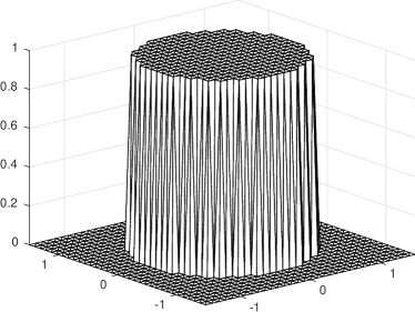
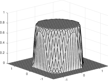
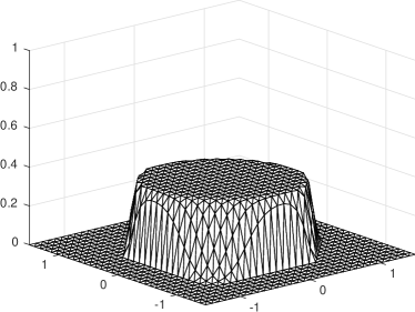
Figure 1. Numerical solutions for $t\approx 0.0,0.1,0.2,0.3$ in Example 5.1 computed with the implicit scheme and $\varepsilon=0$.

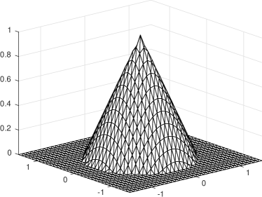
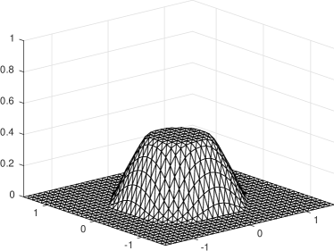
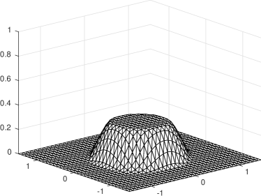
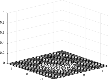
Figure 2. Numerical solutions for $t\approx 0.0,0.05,0.1,0.15$ in Example 5.2 computed with the implicit scheme and $\varepsilon=0$.

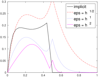
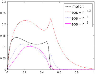
Figure 3. $L^{2}$ errors as functions of $t\in[0,1]$ in Example 5.1 for the semi-implicit scheme with $\varepsilon=h^{\alpha}$, $\alpha=1/2,1,2$, and implicit approximations on triangulations $\mathcal{T}_{\ell}$, $\ell=4$ (left) and $\ell=5$ (right).

$\ell$	implicit	${\varepsilon=h^{1/2}}$	${\varepsilon=h}$	${\varepsilon=h^{2}}$
3	0.3135	0.4024	0.2515	0.1342
4	0.1999	0.3179	0.1495	0.1197
5	0.1421	0.2276	0.1139	0.1030
6	0.1313	0.1882	0.1005	0.0980
7	–	0.1487	0.0813	0.0786
8	–	0.1172	0.0701	0.0679
9	–	0.0908	0.0595	0.0576
10	–	0.0710	0.0510	0.0496

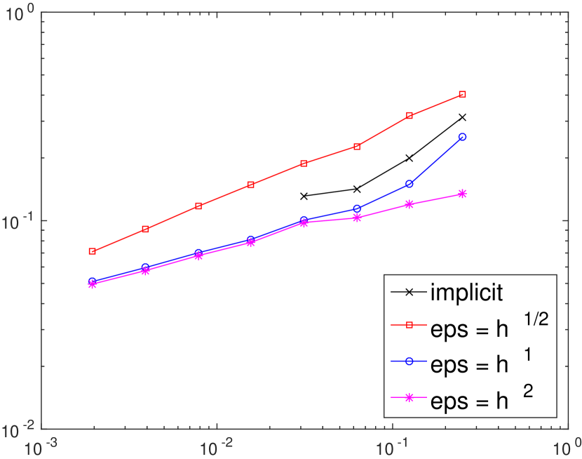
Figure 4. Maximal $L^{2}$ errors for different choices of $\varepsilon$ and on different triangulations $\mathcal{T}_{\ell}$ of level $\ell$ in Example 5.1.

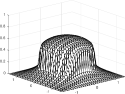
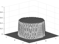
Figure 5. Numerical approximations at $t\approx 0.2$ for $\varepsilon=h^{\alpha}$, $\alpha=1/2,1,2$ (left to right) in Example 5.1. In comparison with the solution obtained with the implicit scheme shown in Figure 1 we observe a smoothing of the discontinuity.

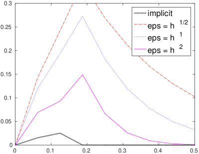
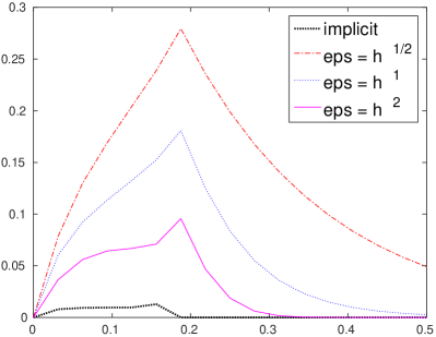
Figure 6. $L^{2}$ errors as functions of $t\in[0,1]$ in Example 5.2 for the semi-implicit scheme with $\varepsilon=h^{\alpha}$, $\alpha=1/2,1,2$, and implicit approximations on triangulations $\mathcal{T}_{\ell}$, $\ell=4$ (left) and $\ell=5$ (right).

$\ell$	implicit	${\varepsilon=h^{1/2}}$	${\varepsilon=h}$	${\varepsilon=h^{2}}$
3	0.1100	0.3368	0.2936	0.1809
4	0.0753	0.3432	0.2729	0.1490
5	0.0129	0.2795	0.1808	0.0956
6	0.0066	0.2169	0.1087	0.0588
7	–	0.1615	0.0617	0.0364
8	–	0.1161	0.0341	0.0241
9	–	0.0814	0.0186	0.0149
10	–	0.0585	0.0101	0.0089

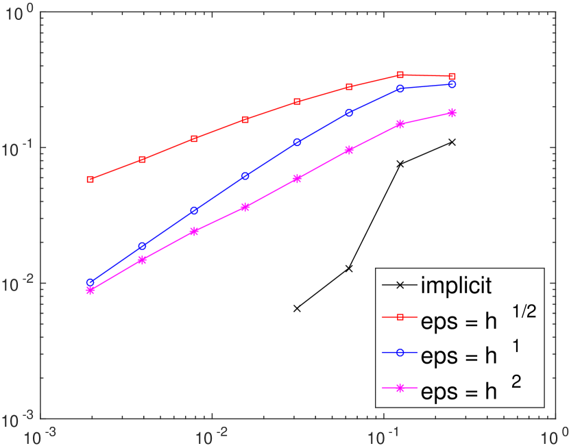
Figure 7. Maximal $L^{2}$ errors for different choices of $\varepsilon$ and on different triangulations $\mathcal{T}_{\ell}$ of level $\ell$ in Example 5.2.

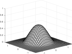
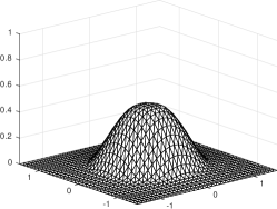
Figure 8. Numerical approximations at $t\approx 0.1$ for $\varepsilon=h^{\alpha}$, $\alpha=1/2,1,2$ (left to right) in Example 5.2. In comparison with the solution obtained with the implicit scheme shown in Figure 2 we observe a rounding of the kinks.

5.B. Experimental observations

We computed numerical approximations with implicit and the semi-implicit schemes on sequences of quasi-uniform triangulations with mesh-size $h$, using different regularization parameters $\varepsilon$, and the fixed relation $\tau=h/4$.

5.B.1. Results for Example 5.1

In Figure 3 we plotted the $L^{2}$ errors for the implicit and the semi-implicit schemes with regularization parameters $\varepsilon=h^{\alpha}$, $\alpha=1,1/2,2$, as functions of $t\in[0,T]$, $T=1$, obtained for the triangulations $\mathcal{T}_{4}$ and $\mathcal{T}_{5}$. We observe that the $L^{2}$ errors decrease monotonically with $\varepsilon$ during most of the evolution with a certain stagnation, and that the errors obtained with the implicit scheme are comparable as long as the solution is nontrivial. In particular, the implicit scheme predicts accurately the extinction time $t=0.5$ in contrast to the approximations obtained with the regularized, semi-implicit method. The maximal $L^{2}$ errors on $t\in[0,T]$ for several triangulations of decreasing mesh size displayed in Figure 4 show that for a larger value of $\varepsilon$ we obtain a better experimental convergence rate. This confirms the critical dependence of our error estimates on the regularization parameter $\varepsilon$. No clear experimental convergence rate can be deduced for the implicit approach although we used a stringent stopping criterion (residual less than $\delta_{\rm stop}=h^{5}$ in the $\ell^{2}$-norm). This condition is dictated by theory of the alternating direction method of multipliers (ADMM) of [BM17], and guarantees that the computational results are not due to poor resolution, but prevents ADMM from converging beyond 6 uniform refinements, namely for $h\leq 5\cdot 10^{-2}$. Figure 5 displays snapshots of numerical solutions on the same triangulation $\mathcal{T}_{5}$ but with different regularization parameters $\varepsilon$ at $t\approx 0.2$. As expected, the smearing effect across the jump discontinuity set of the exact solution depends on $\varepsilon$. The choice $\varepsilon=h^{2}$ appears to give very accurate approximations on $\mathcal{T}_{5}$ although, as depicted in Figure 4, it exhibits the worse experimental convergence rate.

5.B.2. Results for Example 5.2

The results of our numerical experiments shown in Figures 6, 7, and 8 are similar to those for Example 5.1. Here, we observe the best experimental convergence rate for the choice $\varepsilon=h$ instead of $\varepsilon=h^{1/2}$ which may be explained by the uniform Lipschitz continuity of the solution. The implicit treatment leads to smaller approximation errors but, as in Example 5.1, the stringent stopping criterion for ADMM prevents its convergence beyond six uniform mesh refinements.

5.B.3. Conclusions

Our numerical experiments confirm that the error estimates for the semi-implicit scheme depend on the inverse of the regularization parameter $\varepsilon$. The experimental convergence rates are better than those predicted by theory: for $\tau$ proportional to $h$ we expect no convergence (see Corollary 4.3). This feature appears to be related to special regularity properties of the explicit solutions such as $\partial_{t}u(t)\in L^{\infty}(\Omega)$ and $u(t)\in W^{1,\infty}(\Omega)$ for all $t\in(0,T)$ in Examples 5.1 and 5.2, respectively. The implicit scheme leads to highly accurate approximations that provide good predictions of extinction times, but require a substantially larger computational effort. In fact, finding reliable stopping criteria for the iterative solver, the alternating direction method of multipliers, is a challenging task. Therefore, the semi-implicit scheme may also be applied as iterative solver for each time step of the implicit scheme.

Acknowledgments. SB and RHN acknowledge hospitality of the Hausdorff Research Institute for Mathematics within the trimester program Multiscale Problems: Algorithms, Numerical Analysis and Computation. RHN was partially supported as Simons Visiting Professor, in connection with the Oberwolfach Workshop Emerging Developments in Interfaces and Free Boundaries, as well as by the NSF grant DMS-1411808. SB also acknowledges support by the DFG priority programme SPP-1962.

References

• [Bar15] Sören Bartels, Numerical methods for nonlinear partial differential equations, Springer Series in Computational Mathematics, vol. 47, Springer, Cham, 2015.
• [Bar16] by same author, Broken Sobolev space iteration for total variation regularized minimization problems, IMA J. Numer. Anal. 36 (2016), no. 2, 493–502.
• [BCN02] Giovanni Bellettini, Vicent Caselles, and Matteo Novaga, The total variation flow in $\mathbb{R}^{N}$, J. Differential Equations 184 (2002), no. 2, 475–525.
• [BDF12] Dominic Breit, Lars Diening, and Martin Fuchs, Solenoidal Lipschitz truncation and applications in fluid mechanics, J. Differential Equations 253 (2012), no. 6, 1910–1942.
• [BDR15] Luigi C. Berselli, Lars Diening, and Michael Růžička, Optimal error estimate for semi-implicit space-time discretization for the equations describing incompressible generalized Newtonian fluids, IMA J. Numer. Anal. 35 (2015), no. 2, 680–697.
• [BL93] John W. Barrett and Wen Bin Liu, Finite element approximation of the $p$-Laplacian, Math. Comp. 61 (1993), no. 204, 523–537.
• [BL94] by same author, Finite element approximation of the parabolic $p$-Laplacian, SIAM J. Numer. Anal. 31 (1994), no. 2, 413–428.
• [BM17] Sören Bartels and Marijo Milicevic, Alternating direction method of multipliers with variable step sizes, ArXiv e-prints (2017), no. 1704.06069.
• [BNS14] Sören Bartels, Ricardo H. Nochetto, and Abner J. Salgado, Discrete total variation flows without regularization, SIAM J. Numer. Anal. 52 (2014), no. 1, 363–385.
• [BNS15] by same author, A total variation diminishing interpolation operator and applications, Math. Comp. 84 (2015), no. 296, 2569–2587.
• [Bré73] Haim Brézis, Opérateurs maximaux monotones et semi-groupes de contractions dans les espaces de Hilbert, North-Holland Publishing Co., Amsterdam-London; American Elsevier Publishing Co., Inc., New York, 1973, North-Holland Mathematics Studies, No. 5. Notas de Matemática (50).
• [Cha04] Antonin Chambolle, An algorithm for mean curvature motion, Interfaces Free Bound. 6 (2004), no. 2, 195–218.
• [DDE05] Klaus Deckelnick, Gerhard Dziuk, and Charles M. Elliott, Computation of geometric partial differential equations and mean curvature flow, Acta Numer. 14 (2005), 139–232.
• [DE08] Lars Diening and Frank Ettwein, Fractional estimates for non-differentiable elliptic systems with general growth, Forum Math. 20 (2008), no. 3, 523–556.
• [DER07] Lars Diening, Carsten Ebmeyer, and Michael Růžička, Optimal convergence for the implicit space-time discretization of parabolic systems with $p$-structure, SIAM J. Numer. Anal. 45 (2007), no. 2, 457–472.
• [DFW17] Lars Diening, Massimo Fornasier, and Maximilian Wank, A relaxed Kačanov iteration for the $p$-Poisson problem, ArXiv e-prints (2017).
• [Dzi99] Gerd Dziuk, Numerical schemes for the mean curvature flow of graphs, Variations of domain and free-boundary problems in solid mechanics (Paris, 1997), Solid Mech. Appl., vol. 66, Kluwer Acad. Publ., Dordrecht, 1999, pp. 63–70.
• [Eyr36] Henry Eyring, Viscosity, plasticity, and diffusion as examples of absolute reaction rates, The Journal of Chemical Physics 4 (1936), no. 4, 283–291.
• [FV03] Francesca Fierro and Andreas Veeser, A posteriori error estimators for regularized total variation of characteristic functions, SIAM J. Numer. Anal. 41 (2003), no. 6, 2032–2055.
• [FvOP05] Xiaobing Feng, Markus von Oehsen, and Andreas Prohl, Rate of convergence of regularization procedures and finite element approximations for the total variation flow, Numer. Math. 100 (2005), no. 3, 441–456.
• [NSV00] Ricardo H. Nochetto, Giuseppe Savaré, and Claudio Verdi, A posteriori error estimates for variable time-step discretizations of nonlinear evolution equations, Comm. Pure Appl. Math. 53 (2000), no. 5, 525–589.
• [Rul96] Jim Rulla, Error analysis for implicit approximations to solutions to Cauchy problems, SIAM J. Numer. Anal. 33 (1996), no. 1, 68–87.