Transformational Sparse Coding

Abstract

A fundamental problem faced by object recognition systems is that objects and their features can appear in different locations, scales and orientations. Current deep learning methods attempt to achieve invariance to local translations via pooling, discarding the locations of features in the process. Other approaches explicitly learn transformed versions of the same feature, leading to representations that quickly explode in size. Instead of discarding the rich and useful information about feature transformations to achieve invariance, we argue that models should learn object features conjointly with their transformations to achieve equivariance. We propose a new model of unsupervised learning based on sparse coding that can learn object features jointly with their affine transformations directly from images. Results based on learning from natural images indicate that our approach matches the reconstruction quality of traditional sparse coding but with significantly fewer degrees of freedom while simultaneously learning transformations from data. These results open the door to scaling up unsupervised learning to allow deep feature+transformation learning in a manner consistent with the ventral+dorsal stream architecture of the primate visual cortex.

1 Introduction

A challenging problem in computer vision is the reliable recognition of objects under a wide range of transformations. Approaches such as deep learning that have achieved success in recent years usually require large amounts of labeled data, whereas the human brain has evolved to solve the problem using an almost unsupervised approach to learning object representations. During early development, the brain builds an internal representation of objects from unlabeled images that can be used in a wide range of tasks.

Much of the complexity in learning efficient and general-purpose representations comes from the fact that objects can appear in different poses, at different scales, locations, orientations and lighting conditions. Models have to account for these transformed versions of objects and their features. Current successful approaches to recognition use pooling to allow limited invariance to two-dimensional translations (Ranzato et al. (2007)). At the same time pooling discards information about the location of the detected features. This can be problematic because scaling to large numbers of objects requires modeling objects in terms of parts and their relative pose, requiring the pose information to be retained.

Previous unsupervised learning techniques such as sparse coding (Olshausen & Field (1997)) can learn features similar to the ones in the visual cortex but these models have to explicitly learn large numbers of transformed versions of the same feature and as such, quickly succumb to combinatorial explosion, preventing hierarchical learning. Other approaches focus on computing invariant object signatures (Anselmi et al. (2013; 2016)), but are completely oblivious to pose information.

Ideally, we want a model that allows object features and their relative transformations to be simultaneously learned, endowing itself with a combinatorial explanatory capacity by being able to apply learned object features with object-specific transformations across large numbers of objects. The goal of modeling transformations in images is two-fold: (a) to facilitate the learning of pose-invariant sparse feature representations, and (b) to allow the use of pose information of object features in object representation and recognition.

We propose a new model of sparse coding called transformational sparse coding that exploits a tree structure to account for large affine transformations. We apply our model to natural images. We show that our model can extract pose information from the data while matching the reconstruction quality of traditional sparse coding with significantly fewer degrees of freedom. Our approach to unsupervised learning is consistent with the concept of “capsules” first introduced by Hinton et al. (2011), and more generally, with the dorsal-ventral (features+transformations) architecture observed in the primate visual cortex.

2 Transformational Sparse Coding

2.1 Transformation Model

Sparse coding (Olshausen & Field (1997)) models each image $I$ as a sparse combination of features:

$$I\simeq Fw\>\>\>\text{s.t. w is sparse}$$

Sparsity is usually enforced by the appropriate penalty. A typical choice is $S_{1}(w)=\|w\|_{1}$. We can enhance sparse coding with affine transformations by transforming features before combining them. The vectorized input image $I$ is then modeled as:

$$I=\sum_{k=1}^{K}w_{k}T(x_{k})F_{k}$$

where $w_{k},F_{k}$ denote the $k$-th weight specific to the image and the $k$-th feature respectively and $T(x_{k})$ is a feature and image specific transformation.

In modeling image transformations we follow the approach of Rao & Ruderman (1999) and Miao & Rao (2007). We consider the $2$D general affine transformations. These include rigid motions such as vertical and horizontal translations and rotations, as well as scaling, parallel hyperbolic deformations along the $X/Y$ axis and hyperbolic deformations along the diagonals. A discussion on why these are good candidates for inclusion in a model of visual perception can be found in Dodwell (1983). Figure 5 in Appendix A shows the effects of each transformation.

Any subset of these transformations forms a Lie group with the corresponding number of dimensions ($6$ for the full set). Any transformation in this group can be expressed as the matrix exponential of a weighted combination of matrices (the group generators) that describe the behaviour of infinitesimal transformations around the identity:

$$T(x)=e^{\sum_{j}x_{j}G_{j}}$$

For images of $M$ pixels, $T(x)$ is a matrix of size $M\times M$. Note that the generator matrices and the features used are common across all images. The feature weights and transformation parameters can be inferred (and the features learned) by gradient descent on the regularized MSE objective:

$$L(w,x,F)=\frac{1}{N}\sum_{i=1}^{N}\left\|I_{i}-\sum_{k=1}^{K}w_{ik}T(x_{ik})F_{k}\right\|_{2}^{2}+\lambda_{w}S_{1}(w)+\lambda_{F}\|F\|_{2}^{2}$$

Although this model ties sparse coding with transformations elegantly, learning large transformations with it is intractable. The error surface of the loss function is highly non-convex with many shallow local minima. Figures 1,1,1 show the surface of $L$ as a function of horizontal and vertical translation, horizontal translation and rotation and vertical translation and rotation parameters. The model tends to settle for small transformations around the identity. Due to the size of the parameters that we need to maintain, a random restart approach would be infeasible.

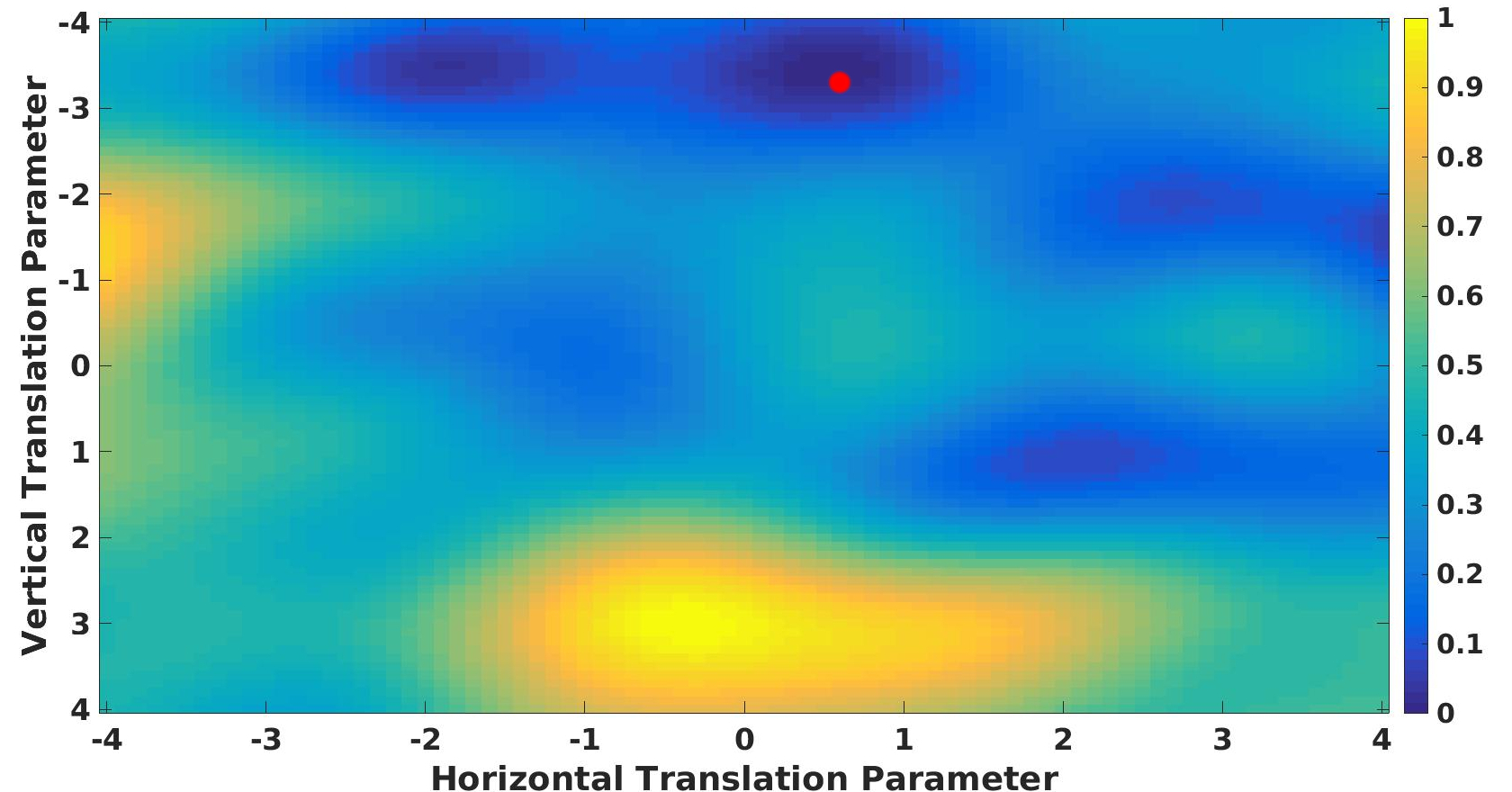
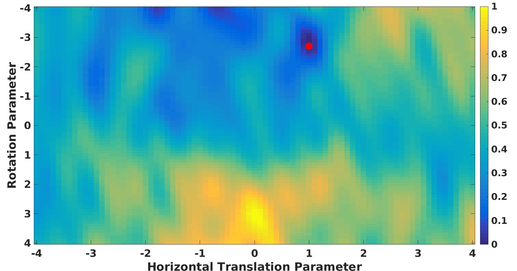
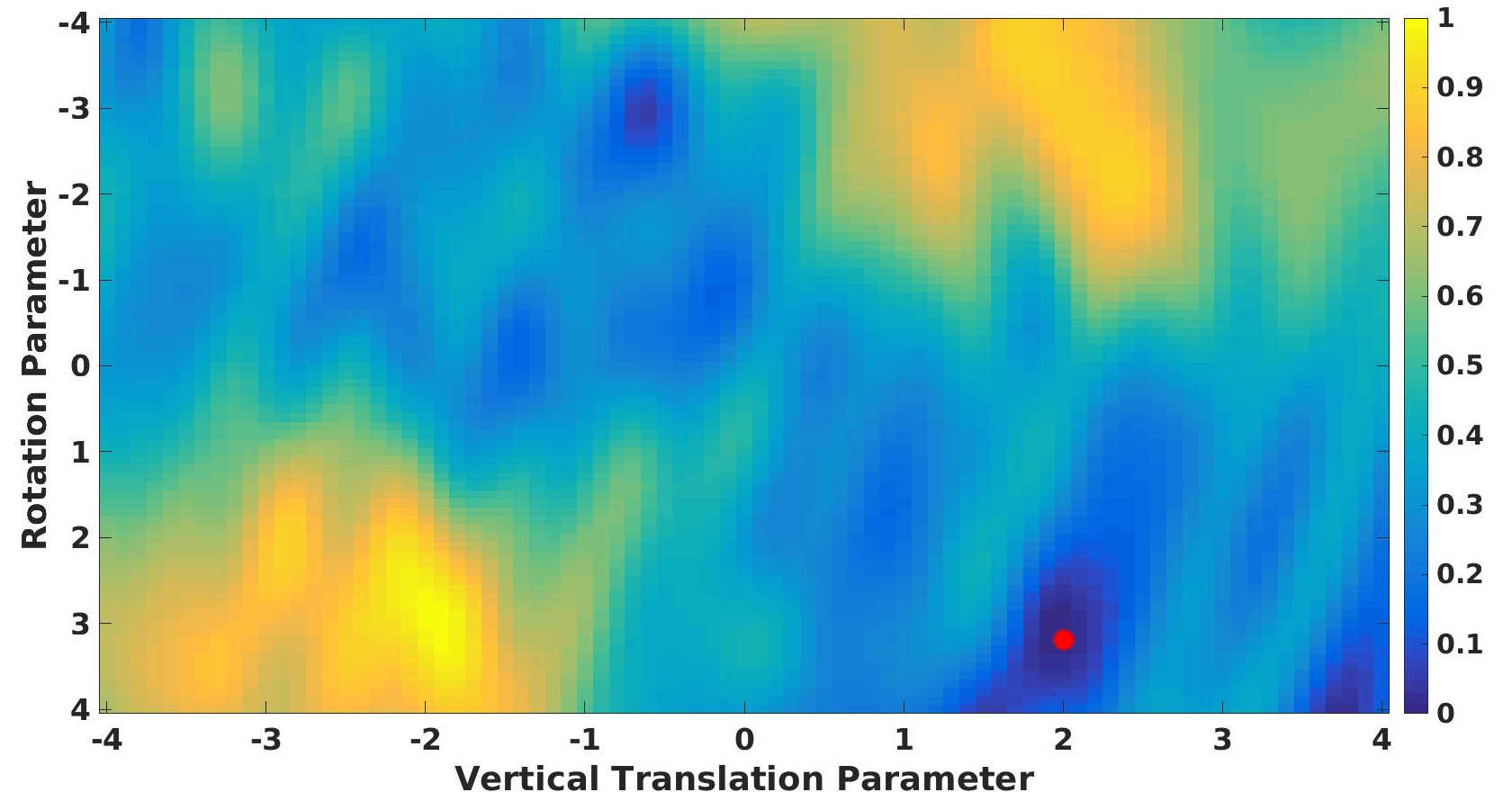
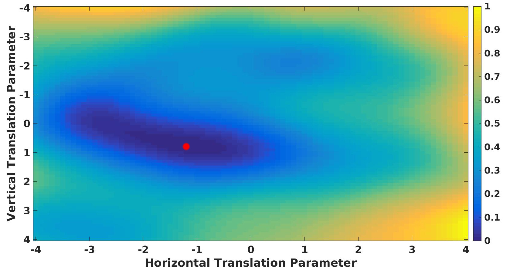
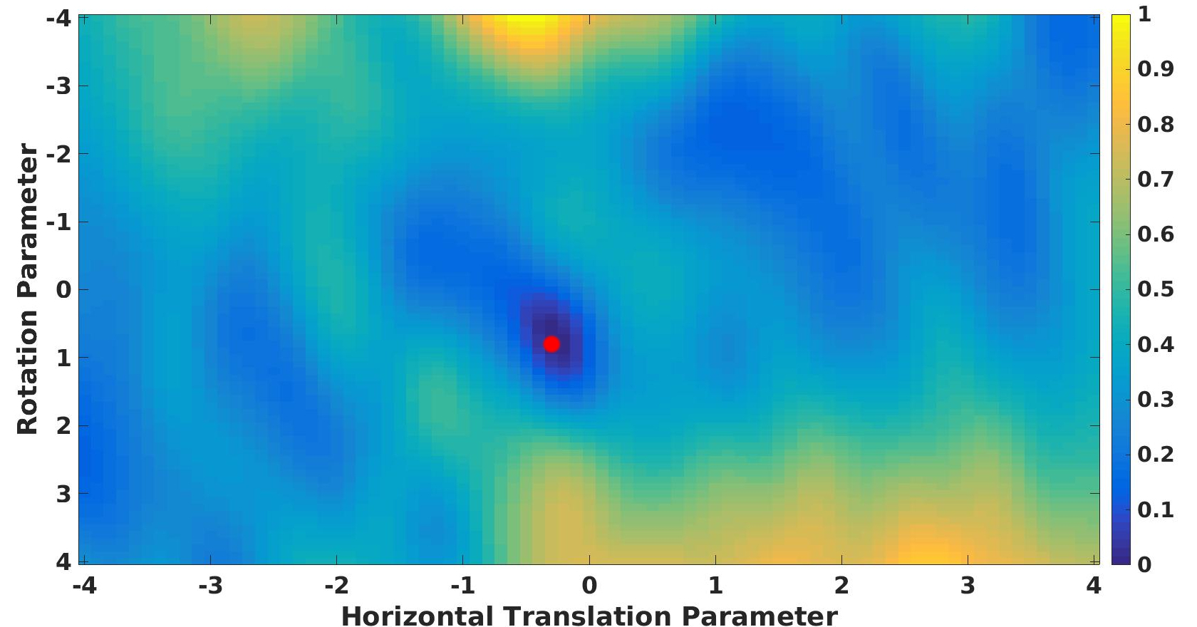
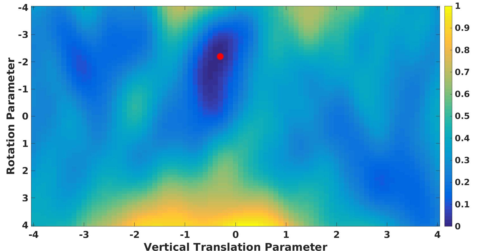
Figure 1: Normalized reconstruction error for individual vs. batch $8\times 8$ natural image patches. (a),(b),(c) show the surface of the reconstruction error for horizontal and vertical translations, horizontal translations and rotation, vertical translations and rotations for an individual data point and feature. (d),(e),(f) show the same, averaged over a batch of $2000$ data points. The error is normalized between $0$ and $1$ for comparison. The global minimum in the range is marked in red. In the batch case, averaging makes the error surface smoother and learning easier.

2.2 Transformation Trees

We introduce Transformational Sparse Coding Trees to circumvent this problem using hierarchies of transformed features. The main idea is to gradually marginalize over an increasing range of transformations. Each node in the tree represents a feature derived as a transformed version of its parent, with the root being the template of the feature. The leaves are equivalent to a set of sparse basis features and are combined to reconstruct the input as described above. A version of the model using a forest of trees of depth one (flat trees), is given by:

$$I\simeq\sum_{v=1}^{V}\sum_{b\sim ch(v)}w_{b}U_{b}$$

where $U_{b}=T(x_{v\rightarrow b})F_{v}$ and $ch(v)$ the children of root $v$. The feature $U_{b}$ is a leaf, derived from the root feature $F_{v}$ via the fixed (across all data-points) transformation $T(x_{v\rightarrow b})$. Deeper trees can be built accordingly (Section 3.3). A small example of a tree learned from natural image patches is shown in Figure 2.

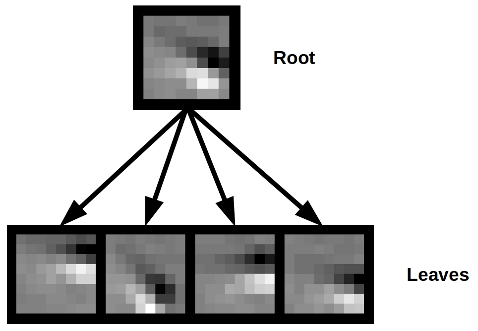
Figure 2: Example of a tree learned from natural image patches. The leaves correspond to rigid transformations of the root.

There are multiple advantages to such a hierarchical organization of sparse features. Some transformations are more common in data than others. Each path in the tree corresponds to a transformation that is common across images. Such a path can be viewed as a “transformation feature” learned from the data. Each additional node in the tree “costs” a fixed set of new parameters equal in size to the dimensions of the underlying Lie group (six in our case). At the same time the node contributes a whole new feature to the sparse code. Averaging over many data points, smoothens the surface of the error function and makes larger transformations more accessible to optimization. Figures 1,1,1 show the error surface averaged over a batch of $2000$ patches.

For every leaf that is activated, the root template represents the identity of the feature and the transformation associated with the path to the root, the pose. In other words the tree is an equivariant representation of the feature over the parameter region defined by the set of paths to the leaves, very similar to the concept of a capsule introduced by Hinton et al. (2011). In fact, every increasing subtree corresponds to a capsule of increasing size.

2.3 Learning

The reconstruction mean squared-error (MSE) for a forest of flat trees is given by:

$$L_{MSE}(w,x,F)=\frac{1}{N}\sum_{i=1}^{N}\left\|I_{i}-\sum_{v=1}^{V}\sum_{b\sim ch(v)}w_{ib}T(x_{v\rightarrow b})F_{v}\right\|_{2}^{2}$$

Increasing the feature magnitudes and decreasing the weights will result in a decrease in loss. We constraint the root feature magnitudes to be of unit $\ell_{2}$ norm. Consider different, transformed, versions of the same root template. For every such version there is a set of tree parameters that compensates for the intrinsic transformation of the root and results in the same leaves. To make the solution unique we directly penalize the transformation parameter magnitudes. Since scaling and parallel deformation can also change the magnitude of the filter, we penalize them more to keep features/leaves close to unit norm. The full loss function of the model is:

$$L(w,x,F)=L_{MSE}(w,x,F)+\lambda_{w}S_{1}(w)+\sum_{j=1}^{6}\lambda_{j}X_{[j]}$$

s.t.

$$\forall v,\|F_{v}\|_{2}=1$$

where $X_{[j]}$ is the vector of the collective parameters for generator $G_{j}$.

Lee et al. (2007) use an alternating optimization approach to sparse coding. First the weights are inferred using the feature sign algorithm and then the features are learned using a Lagrange dual approach. We use the same approach for the weights. Then we optimize the transformation parameters using gradient descent. The root features can be optimized using the analytical solution and projecting to unit norm.

The matrix exponential gradient $\frac{\partial L}{\partial x}$ can be computed using the following formula (Ortiz et al. (2001)):

$$\frac{\partial e^{A(t)}}{\partial t}=\int_{0}^{1}e^{\alpha A(t)}\frac{\partial A(t)}{\partial t}e^{(1-\alpha)A(t)}d\alpha$$

The formula can be interpreted as:

$$E_{\alpha\sim U(0,1)}\left[D(\alpha)\right]$$

where $D(\alpha)=e^{\alpha A(t)}\frac{\partial A(t)}{\partial t}e^{(1-\alpha)A(t)}$. For our experiments we approximated the gradient by drawing a few samples $\{\tilde{\alpha}_{s}\}_{s=1}^{S}$ and computing $E_{\tilde{\alpha}}\left[D(\tilde{\alpha})\right]$. This can be regarded as a stochastic version of the approach used by Culpepper & Olshausen (2009).

Some features might get initialized near shallow local optima (i.e. close to the borders or outside the receptive field). These features eventually become under-used by the model. We periodically check for under-used features and re-initialize their transformation parameters . For re-initialization we select another feature in the same tree at random with probability proportional to the fraction of data points that used it in that batch. We then reset the transformation parameters at random, with small variance and centered around the chosen filter’s parameters.

3 Experiments

3.1 Learning Representations

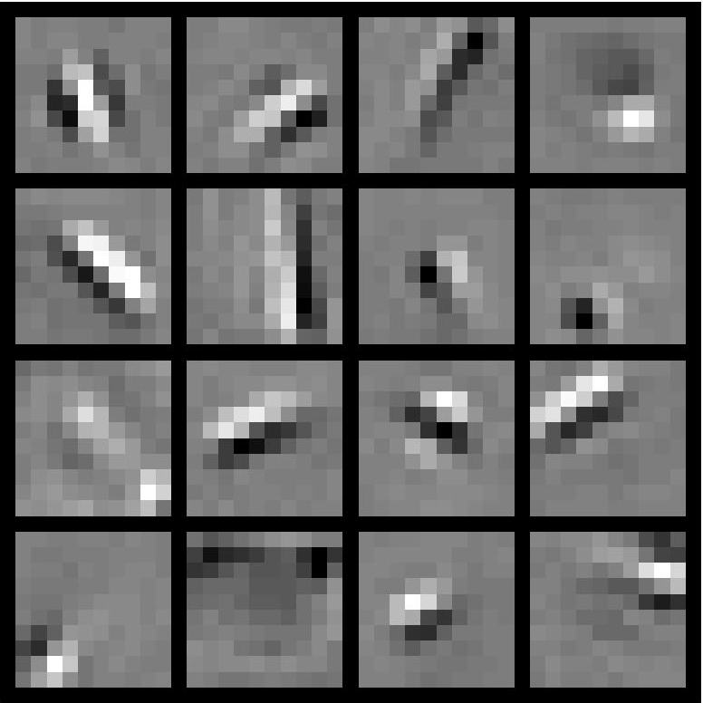
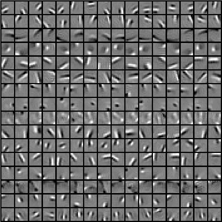
Figure 7: Learned features for $16$ trees with branching factor $16$. Each row corresponds to leaves/transformations of the same root.

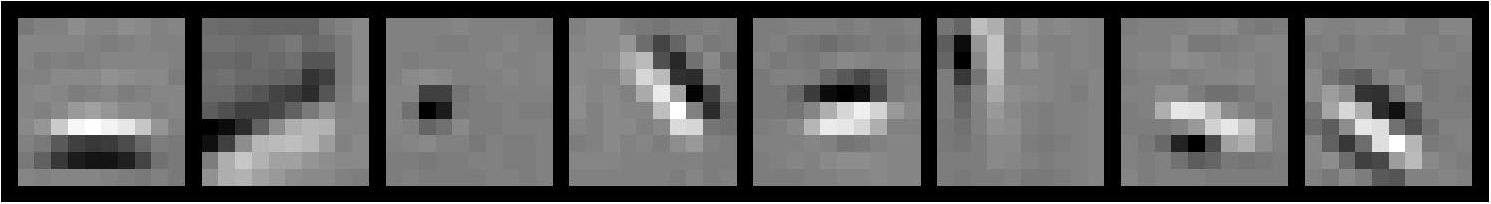
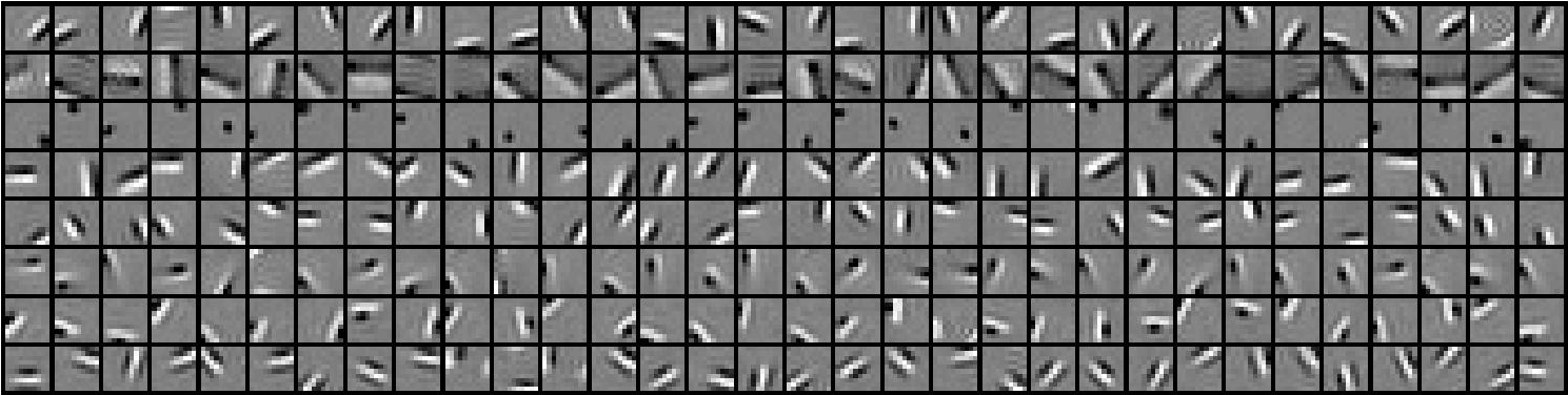
Figure 8: Learned features for $8$ trees with branching factor $32$. Each row corresponds to leaves/transformations of the same root.

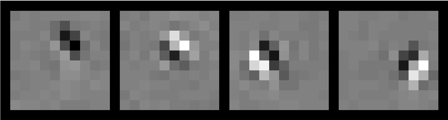
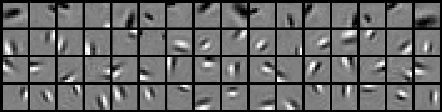
Figure 9: Learned features for $4$ trees with branching factor $16$. Each row corresponds to leaves/transformations of the same root.

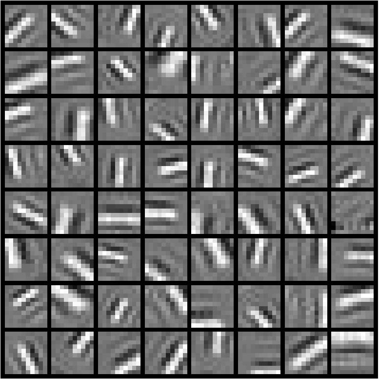
Figure 10: Learned features for $1$ tree with branching factor $64$. All features are transformations of the same root.

We apply transformational sparse coding (TSC) with forests of flat trees to natural image patches. Our approach allows us to learn features resembling those of traditional sparse coding. Apart from reconstructing the input, the model also extracts transformation parameters from the data. Figure 3 shows a reconstruction example. Figure 4 shows the root features learned from $10\times 10$ natural image patches using a forest of size $8$ with branching factor $8$, equipped with the full six-dimensional group. The forest has a total of $64$ features. Figure 4 shows the features corresponding to the roots. Figure 4 shows the corresponding leaves. Each row contains features derived from the same root. More examples of learned features are shown in Figures 7, 8, 9 and 10 in Appendix C.

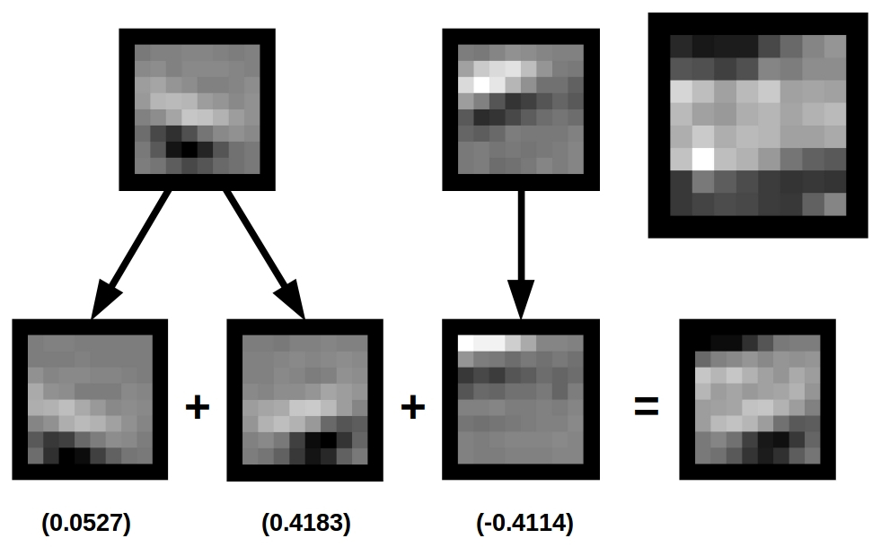
Figure 3: Reconstruction example. The root features are transformed and combined with different weights to reconstruct (bottom right) the $8\times 8$ natural image patch in the top right corner.

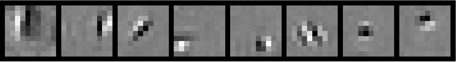
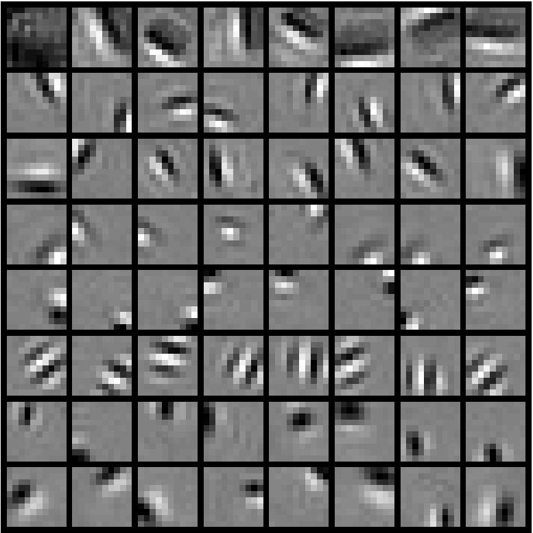
Figure 4: Learned features for $8$ trees with a branching factor of $8$. (a) Features corresponding to the roots. (b) Features/Leaves: Each row corresponds to leaves/transformations of the same root.

3.2 Comparison with Sparse Coding

Even though derivative features have to be explicitly constructed for inference, the degrees of freedom of our model are significantly lower than that of traditional sparse coding. Specifically:

$$df_{TSC}=(\text{\# of roots})\times\left(\text{\# of pixels}-1+\text{branching factor}\times\text{group dimension}\right)$$

whereas:

$$df_{SC}=\text{\# of features}\times\left(\text{\# of pixels}-1\right)$$

Note that the group dimension is equal to $3$ for rigid motions and $6$ for general $2$D affine transformations.

We compare transformational sparse coding forests of various layouts and choices for $\lambda_{w}$ with traditional sparse coding on $10\times 10$ natural image patches. Some transformations change the feature magnitudes and therefore the sparsity pattern of the weights. To make the comparison clearer, for each choice of layout and penalty coefficient, we run sparse coding, constraining the feature magnitudes to be equal to the average feature magnitude of our model. The results are shown in Table 1. The reconstruction error of our model is close to that of sparse coding, albeit with slightly less sparse solutions, even though it has significantly fewer degrees of freedom. Our model extracts pose information in the form of group parameters.

Table 1: Comparison of transformational sparse coding (TSC) with sparse coding (SC) for $10\times 10$ natural image patches. We compare the error (MSE) and the degrees of freedom ($df$) over $40000$ data points. “Sparsity” is the average number of non-zero weights. $\lambda_{w}$ is the penalty coefficient for the weights and controls the sparseness of the solution.

	TSC				SC
$\lambda_{w}$	Layout	MSE	Sparsity	$df_{TSC}$	MSE	Sparsity	$df_{SC}$	# of features	$\frac{df_{SC}}{df_{TSC}}$
0.4	$1\times 64$	2.13	13.3	447	1.71	12.3	6336	64	14.17
0.5	$1\times 128$	2.28	12.1	867	1.96	10.3	12672	128	14.62
0.4	$8\times 8$	1.89	13.3	1176	1.72	12.5	6336	64	5.38
0.4	$4\times 16$	1.91	13.3	780	1.69	12.3	6336	64	8.12
0.5	$8\times 8$	2.36	10.4	1176	2.15	9.9	6336	64	5.38
0.5	$4\times 16$	2.38	11	780	2.12	10.0	6336	64	8.12
0.4	$16\times 16$	1.66	14.3	3120	1.56	13.2	25344	256	8.12
0.4	$8\times 32$	1.67	14.6	2328	1.56	13.2	25344	256	10.88

3.3 Deeper Trees

We can define deeper trees by associating a set of transformation parameters with each branch. These correspond to additive contributions to the complete transformation that yields the leaf when applied to the root:

$$I_{i}\simeq\sum_{v=1}^{V}\sum_{b\sim ch(v)}w_{ib}T(x_{P})F_{v}$$

where $x_{P}=\sum_{e\in\text{path}(b,v)}x_{e}$. Optimizing deeper trees is more demanding due to the increased number of parameters. Their advantage is that they lend structure to model. The parameters corresponding to the subtree of an internal node tend to explore the parameter subspace close to the transformation defined by that internal node. In tasks where it is disadvantageous to marginalize completely over transformations, equivariant representations corresponding to intermediate tree layers can be used. An example of such structure is shown in Figure 6 in Appendix B.

4 Related Work

Sohl-Dickstein et al. (2010) present a model for fitting Lie groups to video data. Their approach only works for estimating a global transformation between consecutive video frames. They only support transformations of a single kind (ie only rotations). Different such single-parameter transformations have to be chained together to produce the global one. The corresponding transformation parameters also have to be inferred and stored in memory and cannot be directly converted to parameters of a single transformation. Kokiopoulou & Frossard (2009) present an approach to optimally estimating transformations between pairs of images. They support rigid motions and isotropic scaling. Culpepper & Olshausen (2009) focus on learning the group operators and transformation parameters from pairs of images, but do not learn features from data. Our model supports all six transformations and learns object parts and their individual transformations. In contrast with those approaches, our model learns object parts jointly with their transformations within the same image. Our model utilizes the full, six-dimensional, general affine Lie group and captures the pose of each object part in the form of a single set of six transformation parameters.

Grimes & Rao (2005) propose a bilinear model that combines sparse coding with transformations. The model accounts for global transformations that apply to the entire image region. Our model accounts for individual transformations of image parts. Rao & Ballard (1998) propose a model that captures small image transformations with Lie groups using a first-order Taylor approximation. Our model estimates larger transformations of image parts using the full exponential model. Rao & Ruderman (1999) and Miao & Rao (2007) use a first-order Taylor approximation to learn the group operators and the transformation parameters for small transformations.

The work closest to ours is that of Hinton et al. (2011) on capsules. A capsule learns to recognize its template (feature) over a wide range of poses. The pose is computed by a neural network (encoder). The decoder, resembling a computer graphics engine combines the capsule templates in different poses to reconstruct the image. Each transformational sparse coding tree can be thought of as capsule. The template corresponds to the root. The tree learns to “recognize” transformed versions of that template. Our work arrives at the concept of a capsule from a sparse coding perspective. A major difference is that our approach allows us to reuse each feature multiple times in different, transformed versions for each data point.

Gens & Domingos (2014) propose a convolutional network that captures symmetries in the data by modeling symmetry groups. Experiments with rigid motions or various affine transformations show reduced sample complexity. Cohen & Welling (2016) propose a convolutional network that can handle translations, reflections and rotations of $90$ degrees. Dieleman et al. (2016) propose a network that handles translations and rotations. All the above are supervised learning models and apart from the first can handle a limited set of transformations. Our model is completely unsupervised, extends sparse coding and can handle all transformations given by the first order differential equation:

$$\frac{\partial I(\theta)}{\partial\theta}=AI(\theta)$$

as described by Rao & Ruderman (1999).

5 Conclusion

In this paper, we proposed a sparse coding based model that learns object features jointly with their transformations, from data. Naively extending sparse coding for data-point specific transformations makes inference intractable. We introduce a new technique that circumvents this issue by using a tree structure that represents common transformations in data. We show that our approach can learn interesting features from natural image patches with performance comparable to that of traditional sparse coding.

Investigating the properties of deeper trees, learning the tree structure dynamically from the data and extending our model into a hierarchy are subjects of ongoing research.

Appendix

A Generator Effects

Figure 5 presents the effects of each individual transformation of the six that are supported by our model. The template is a square 5.

Figure 5: Effects of each individual transformation on the template (a): (b) horizontal translation, (c) vertical translation, (d) rotation, (e) scaling, (f) parallel hyperbolic deformation along the $X/Y$ axis, (g) hyperbolic deformation along the diagonals. To compute the generators, we used the $\operatorname{sinc}$ interpolation function.

B Deeper trees and structure

Figure 6 presents an example of structure learned by deeper trees. This example consists of vertical and horizontal lines. Each image patch is either blank, contains one vertical or one horizontal line or both. A patch is blank with probability $\frac{1}{9}$, contains exactly one line with probability $\frac{2}{3}$ or two lines with probability $\frac{2}{9}$. Each line is then generated at one of eight positions at random. Fitting two binary trees results in some continuity in the features, whereas flat trees provide no such structure.

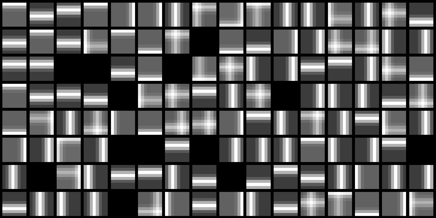
Figure 6: Features learned for the double-line example: (a) Input, (b) features learned by a forest of two flat trees of size eight, (c) features learned by two binary trees of the same size. For (c) the leaves have been reordered with subtree permutations to reveal the order. Each subtree learns features corresponding to an area of the input.

C Learned Features

References

- Anselmi et al. (2013) Fabio Anselmi, Joel Z. Leibo, Lorenzo Rosasco, Jim Mutch, Andrea Tacchetti, and Tomaso A. Poggio. Unsupervised learning of invariant representations in hierarchical architectures. CoRR, abs/1311.4158, 2013. URL http://arxiv.org/abs/1311.4158.
- Anselmi et al. (2016) Fabio Anselmi, Joel Z. Leibo, Lorenzo Rosasco, Jim Mutch, Andrea Tacchetti, and Tomaso Poggio. Unsupervised learning of invariant representations. Theor. Comput. Sci., 633(C):112–121, June 2016. ISSN 0304-3975. doi: 10.1016/j.tcs.2015.06.048. URL http://dx.doi.org/10.1016/j.tcs.2015.06.048.
- Cohen & Welling (2016) Taco S. Cohen and Max Welling. Group equivariant convolutional networks. CoRR, abs/1602.07576, 2016. URL http://arxiv.org/abs/1602.07576.
- Culpepper & Olshausen (2009) Benjamin Culpepper and Bruno A. Olshausen. Learning transport operators for image manifolds. In Y. Bengio, D. Schuurmans, J. D. Lafferty, C. K. I. Williams, and A. Culotta (eds.), Advances in Neural Information Processing Systems 22, pp. 423–431. Curran Associates, Inc., 2009. URL http://papers.nips.cc/paper/3791-learning-transport-operators-for-image-manifolds.pdf.
- Dieleman et al. (2016) Sander Dieleman, Jeffrey De Fauw, and Koray Kavukcuoglu. Exploiting cyclic symmetry in convolutional neural networks. CoRR, abs/1602.02660, 2016. URL http://arxiv.org/abs/1602.02660.
- Dodwell (1983) Peter C. Dodwell. The lie transformation group model of visual perception. Perception & Psychophysics, 34(1):1–16, 1983. ISSN 1532-5962. doi: 10.3758/BF03205890. URL http://dx.doi.org/10.3758/BF03205890.
- Gens & Domingos (2014) Robert Gens and Pedro Domingos. Deep symmetry networks. In Proceedings of the 27th International Conference on Neural Information Processing Systems, NIPS’14, pp. 2537–2545, Cambridge, MA, USA, 2014. MIT Press. URL http://dl.acm.org/citation.cfm?id=2969033.2969110.
- Grimes & Rao (2005) David B. Grimes and Rajesh P. N. Rao. Bilinear sparse coding for invariant vision. Neural Comput., 17(1):47–73, January 2005. ISSN 0899-7667. doi: 10.1162/0899766052530893. URL http://dx.doi.org/10.1162/0899766052530893.
- Hinton et al. (2011) Geoffrey E. Hinton, Alex Krizhevsky, and Sida D. Wang. Transforming auto-encoders. In Proceedings of the 21th International Conference on Artificial Neural Networks - Volume Part I, ICANN’11, pp. 44–51, Berlin, Heidelberg, 2011. Springer-Verlag. ISBN 978-3-642-21734-0. URL http://dl.acm.org/citation.cfm?id=2029556.2029562.
- Kokiopoulou & Frossard (2009) E. Kokiopoulou and P. Frossard. Minimum distance between pattern transformation manifolds: Algorithm and applications. IEEE Transactions on Pattern Analysis and Machine Intelligence, 31(7):1225–1238, July 2009. ISSN 0162-8828. doi: 10.1109/TPAMI.2008.156.
- Lee et al. (2007) Honglak Lee, Alexis Battle, Rajat Raina, and Andrew Y. Ng. Efficient sparse coding algorithms. In B. Schölkopf, J. C. Platt, and T. Hoffman (eds.), Advances in Neural Information Processing Systems 19, pp. 801–808. MIT Press, 2007. URL http://papers.nips.cc/paper/2979-efficient-sparse-coding-algorithms.pdf.
- Miao & Rao (2007) Xu Miao and Rajesh P. N. Rao. Learning the Lie Groups of Visual Invariance. Neural Comput., 19(10):2665–2693, October 2007. ISSN 0899-7667. doi: 10.1162/neco.2007.19.10.2665. URL http://dx.doi.org/10.1162/neco.2007.19.10.2665.
- Olshausen & Field (1997) Bruno A Olshausen and David J Field. Sparse coding with an overcomplete basis set: A strategy employed by v1? Vision research, 37(23):3311–3325, 1997.
- Ortiz et al. (2001) M. Ortiz, R. A. Radovitzky, and E. A. Repetto. The computation of the exponential and logarithmic mappings and their first and second linearizations. International Journal for Numerical Methods in Engineering, 52:1431, December 2001. doi: 10.1002/nme.263.
- Ranzato et al. (2007) Marc’Aurelio Ranzato, Fu-Jie Huang, Y-Lan Boureau, and Yann LeCun. Unsupervised learning of invariant feature hierarchies with applications to object recognition. In Proc. Computer Vision and Pattern Recognition Conference (CVPR’07). IEEE Press, 2007.
- Rao & Ballard (1998) Rajesh P N Rao and Dana H Ballard. Development of localized oriented receptive fields by learning a translation-invariant code for natural images. Network: Computation in Neural Systems, 9(2):219–234, 1998. URL http://www.tandfonline.com/doi/abs/10.1088/0954-898X_9_2_005. PMID: 9861987.
- Rao & Ruderman (1999) Rajesh P. N. Rao and Daniel L. Ruderman. Learning lie groups for invariant visual perception. In Proceedings of the 1998 Conference on Advances in Neural Information Processing Systems II, pp. 810–816, Cambridge, MA, USA, 1999. MIT Press. ISBN 0-262-11245-0. URL http://dl.acm.org/citation.cfm?id=340534.340807.