Abstract

Measuring the eye’s mechanical properties in vivo and with minimally invasive techniques can be the key for individualized solutions to a number of eye pathologies. The development of such techniques largely relies on a computational modelling of the eyeball and, it optimally requires the synergic interplay between experimentation and numerical simulation. In Astrophysics and Geophysics the remote measurement of structural properties of the systems of their realm is performed on the basis of (helio-)seismic techniques. As a biomechanical system, the eyeball possesses normal vibrational modes encompassing rich information about its structure and mechanical properties. However, the integral analysis of the eyeball vibrational modes has not been performed yet. Here we show that the vibrational eigenfrequencies of the human eye fall in the interval 100 Hz – 10 MHz. The eyeball normal modes have frequencies separable from the typical range of phasic physiological phenomena (e.g., respiration, pulse). We find that compressible vibrational modes may release a trace on high frequency changes of the intraocular pressure, while incompressible normal modes could be registered analyzing the scattering pattern that the motions of the vitreous humour leave on the retina. Existing contact lenses with embebed devices operating at high sampling frequency could be used to register the microfluctuations of the eyeball shape we obtain. We advance that an inverse problem to obtain the mechanical properties of a given eye (e.g., Young’s modulus, Poisson ratio) measuring its normal frequencies is doable. These measurements can be done using non-invasive techniques, opening very interesting perspectives to estimate the mechanical properties of eyes in vivo. Future research might relate various ocular pathologies with anomalies in measured vibrational frequencies of the eye.

Author Summary

Inspired by the (helio-)seismic techniques customary employed in Geophysics and Astrophysics, we build the foundations of a novel set of techniques for the remote (non-invasive) measurement of the eyeball biomechanical properties. Employing a simplified model of the human eye, we obtain that the typical normal mode frequencies of the eye fall above 100 Hz. Remarkably, these frequencies are significantly different from other phasic physiological phenomena and can be very likely measured with existing devices. The result is rather robust, as the dependence of the eigenfrequencies on the elastic moduli is very modest in the typical ranges of variations of these parameters for human eyes.

Introduction

Obtaining the mechanical properties of the human eye is fundamental for the future development of artificial materials that can be employed as substitutes for natural tissues [1]. Measuring the eye’s mechanical properties in vivo and with minimally invasive techniques can be the key for individualized solutions to a number of eye pathologies. The development of such techniques largely relies on a computational modelling of the eyeball [2] and, it optimally requires the synergic interplay between experimentation and numerical simulation [3].

The eye is a complex organ consisting of several functional and mutually interacting parts [4]. The most important ones from the mechanical point of view are the cornea, lens, vitreous, sclera and retina. Each of these elements holds distinctive mechanical properties that are closely related to their respective anatomic functionality. Changes in the mechanical properties may entail a number of pathologies or even a loss of functionality [5]. Reciprocally, damage inflicted to a healthy eye may result in changes in its elastic and mechanical properties [6]. The mechanical modelling of the human eye is a field that has gained relevance to rationalize the physiology and pathology of the eye [3]. The field is exponentially developing pace to pace with our ability of implementing more complex models on modern computers [7]. Our knowledge of the mechanical properties of the eye has basically come through three different ways: experimentation, in vivo monitoring, or computational modelling. We develop our work in the later framework.

Measuring the elasticity properties of the different tissues forming an eye is challenging. Very often, the determination of mechanical properties of the eye results from a mechanical interaction with its different parts [8, 9, 10]. In addition to standard mechanical testing, the cornea has been characterized through high-resolution microscopy techniques [11], as well as with the Ocular Response Analyzer [12, 13]. Likewise, multiple studies have examined the overall biomechanical properties of the sclera [14, 15]. Ultrasound biomicroscopy has been used to measure the scleral thickness [16, 17]. Magnetic Resonance Imaging (MRI) techniques applied in vivo resulted inaccurate because of the random eye movement of the patients, though it is possible to use MRI scans to produce 3D models of the corneoscleral shells in post-mortem patients [18].

Novel non-invasive techniques need to be devised to measure the mechanical properties of the eye. Here we show that these properties are related to the normal vibrational modes of the eyeball, i.e., to the periodic variations of matter inside of the eyeball resulting from perturbations with respect to its equilibrium state. We have been inspired by the extensive use of the remote measurements of normal-mode related physical quantities in Geophysics and Astrophysics. For instance, the solar interior is routinely scanned by means of helioseismic techniques, which are based on the measurement of the global resonant oscillations of the Sun [19]. Likewise, employing the principles of asteroseismology, neutron star interiors are proven [20, 21] in an attempt to decipher the equation of state for matter at nuclear densities. We believe that this treatment opens up a new set of techniques for remote measuring of the eyes structural properties.

Materials and Methods

The oscillations under consideration in our model are free elastic vibrations, which we assume may arise when applying generic stresses, e.g., on the sclera or the cornea. We tackle the numerical calculation of the vibrational eigenfrequencies and eigenmodes of the human eye under a number of simplifying assumptions. We model the eyeball as a spherical, homogeneous and isotropic elastic solid ball with axial symmetry. While assuming that the eyeball is axially symmetric is very well justified, the assumptions of homogeneity and isotropy are certainly not the most accurate possible. However, these assumptions serve for the primary purpose of reducing the dependence of the constitutive equation only to two elastic constants or moduli of the eye material: the Young’s modulus $E$, and the Poisson ratio $\sigma$. In this simplified framework, we will compute, first analytically and afterwards numerically, the eigenfrequencies of the model attempting to grasp the essential mechanics of an average human eye.

Results

As we have mentioned above, we model the eyeball as a spherically symmetric, homogeneous and isotropic elastic solid ball (Fig. 1). This simplification allows us to use known analytical solutions (S1 Appendix.) in other physics disciplines (e.g., seismology [22] or gravitational wave physics [23, 24]) to calibrate our numerical code (described in Sect. Numerical code).

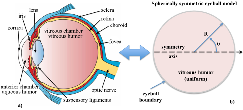
Fig 1: Simplified mechanical model of the eyeball. Left: transversal cut of the human eye with the different structural parts annotated in it (source: Wikipedia). Right: spherically symmetric, homogeneous and isotropic eyeball model employed in this work.

Numerical code

Since we aim to employ non-trivial boundary conditions, we are forced to solve numerically the eigenvalue problem at hand. We have developed a code that solves the eigenvalue problem set by the Navier-Cauchy equation discretizing the eyeball sphere on a two-dimensional grid of nodes in spherical coordinates ($0\leq r\leq R,\>0\leq\theta\leq\pi$). As a first step, we have assumed the elastic moduli to be uniform throughout the spatial grid. However, there is no restriction to implement elastic moduli that depend on the location in the eyeball. This is important because it may enable us to improve the degree of realism of our model for the vibrational modes of the eye, in particular, by using different elastic moduli for the sclera, the cornea, the lens, and the vitreous humour.

First, we will rewrite Eq. (19) for the numerical part with the analytical solutions available in the previous section. In spherical coordinates, and under the assumption of axisymmetry, i.e., neglecting the $\varphi$-dependence, the displacements can be written as

$$u_{i}=(u_{r}(r,\theta),u_{\theta}(r,\theta),u_{\varphi}(r,\theta)),$$

and satisfy the following three equations:

$$-\frac{\mu}{\rho}\Delta u_{r}-\frac{\lambda+\mu}{\rho}u_{j,jr}=p^{2}u_{r}$$ (1)

$$-\frac{\mu}{\rho}\Delta u_{\theta}-\frac{\lambda+\mu}{\rho}u_{j,j\theta}=p^{2}u_{\theta}$$ (2)

$$-\frac{\mu}{\rho}\Delta u_{\varphi}-\frac{\lambda+\mu}{\rho}u_{j,j\varphi}=p^{2}u_{\varphi}.$$ (3)

Under the assumption of axisymmetry, all the derivatives with respect $\varphi$ vanish and Eq. (3) decouples from the other two Equations (1) and (2). We obtain the toroidal modes from the latter equation:

$$-\frac{\mu}{\rho}\Delta u_{\varphi}=p^{2}u_{\varphi}.$$ (4)

with traction boundary conditions, $u_{\varphi,r}=0$. The spheroidal modes result from Equations (1) and (2):

$$-\frac{\mu}{\rho}\Delta u_{r}-\frac{\lambda+\mu}{\rho}\partial_{r}\bigg{[}\frac{1}{r^{2}}\partial_{r}r^{2}u_{r}+\frac{1}{r\sin\theta}\partial_{\theta}\sin\theta u_{\theta}\bigg{]}=p^{2}u_{r}$$ (5)

$$-\frac{\mu}{\rho}\Delta u_{\theta}-\frac{\lambda+\mu}{r\rho}\partial_{\theta}\bigg{[}\frac{1}{r^{2}}\partial_{r}r^{2}u_{r}+\frac{1}{r\sin\theta}\partial_{\theta}\sin\theta u_{\theta}\bigg{]}=p^{2}u_{\theta}$$ (6)

also with traction boundary conditions, $u_{r,r}=0;u_{\theta,r}=0$. Equations (5) and (6) can be cast as an eigenvalue equation, $Lu=\lambda u$, with the vectorial operator

$$Lu:=-\frac{\mu}{\rho}\Delta u_{i}-\frac{\lambda+\mu}{\rho}u_{j,ji}$$ (7)

with $i=r,\theta$, i.e., the equations are coupled due to the axisymmetry hypothesis. If we explicitly insert spherical coordinates, then:

$$Lu=\bigg{(}-\frac{\mu}{\rho}\Delta u_{r}-\frac{\lambda+\mu}{\rho}u_{j,jr},-\frac{\mu}{\rho}\Delta u_{\theta}-\frac{\lambda+\mu}{\rho}u_{j,j\theta}\bigg{)}$$ (8)

and, for clarity, in matrix form we have:

$$\left[\begin{array}[]{cc}a_{rr}&a_{r\theta}\\ a_{\theta r}&a_{\theta\theta}\\ \end{array}\right]\left[\begin{array}[]{c}u_{r}\\ u_{\theta}\\ \end{array}\right]$$ (9)

where expansion of the operator yields:

$$a_{rr} := -\frac{\lambda+2\mu}{\rho}\partial_{rr}-\frac{2(\lambda+2\mu)}{\rho r}\partial_{r}-\frac{\mu}{\rho r^{2}}\partial_{\theta\theta}-\frac{\mu\cot\theta}{\rho r^{2}}\partial_{\theta}+\frac{2(\lambda+2\mu)}{\rho r^{2}}$$ (10)

$$a_{r\theta} := -\frac{(\lambda+\mu)\cot\theta}{\rho r}\partial_{r}+\frac{\lambda+3\mu}{\rho r^{2}}\partial_{\theta}-\frac{\lambda+\mu}{\rho r}\partial_{r\theta}+\frac{\cot\theta(\lambda+3\mu)}{\rho r^{2}}$$ (11)

$$a_{\theta r} := \frac{2(\lambda+2\mu)}{\rho r^{2}}\partial_{\theta}-\frac{\lambda+\mu}{\rho r}\partial_{r\theta}$$ (12)

$$a_{\theta\theta} := -\frac{\mu}{\rho}\partial_{rr}-\frac{2\mu}{\rho r}\partial_{r}+-\frac{\lambda+2\mu}{\rho r^{2}}\partial_{\theta\theta}-\frac{(\lambda+2\mu)\cot\theta}{\rho r^{2}}\partial_{\theta}+\frac{(\lambda+2\mu)\csc^{2}\theta}{\rho r^{2}}$$ (13)

In both types of modes, we compute in a first step the eigenvalues (vibrational frequencies), and in a second step the eigenfunctions (normal displacements). For the eigenvalues we simply compute the zeros of the characteristic polynomial. In practice, working in logarithmic space is advantageous because it reduces the magnitude of coefficients of the polynomial. Knowing the family of eigenvalues, we compute the kernel for each one of them. We substitute each eigenvalue into the corresponding equation, Eq. (4) or Eqs. (5)-(6), obtaining an elliptic equation. With this, we subtract the eigenvalue from the diagonal of the matrix produced by the discretization of the elliptic operator, and proceed further solving the corresponding system of equations by direct numerical inversion of the matrix of the system. As the rank of this matrix cannot be complete, we will obtain the compatible but indeterminate solution as a function of some of the variables (either one or two variables for the toroidal and the spheroidal case, respectively).

Code calibration

We calibrate the code by comparing the frequencies computed with our numerical code and the corresponding analytic values at a density of $\rho=1\,$kg m^-3, an elastic moduli of $E=2.5$ Pa, $\sigma=0.25$ and a radius of the sphere of $R=1\,$m. Note that these values do not correspond to a typical human eye. They are employed for numerical convenience.

As shown in Fig. 2, we get a good agreement in the toroidal ($\varphi-$) case, both in the vibrational patterns and in their corresponding frequencies, demonstrating the ability of the numerical code to recover the analytic values. We point out that agreement improves with a finer mesh encompassing the eyeball (in Fig. 2 we employ a relatively coarse grid of $100\times 50$ points in the $r\times\phi$ directions). A similar analysis has been done for modes where the displacements of the material happen only in the $r-$ and $\theta-$directions (spheroidal modes). The conclusion of both calibration experiments is that our numerical procedure to compute the eigenfrequencies of the system and their displacements is accurate enough.

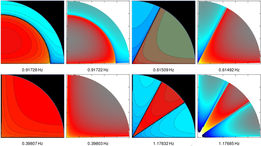
Fig 2: Callibration of the method. Comparison between the analytic (panels with black background) and numerical (white background) solutions of vibrational patterns. Because of the symmetries, only one quadrant of the full equatorial plane of an spherical body is shown. Modes of odd and even parities are displayed in the upper and lower panels, respectively. In this case, we are using 100 points in the radial direction and 50 in the angular one. We can also observe a good agreement in their corresponding frequencies (listed below each panel), that improves as we increase the resolution.

Application of the method to a typical human eye

The exact eigenfrequency values are sensitive to the imposed boundary conditions. We assume that the surface of the eye (either the sclera or the cornea) is free to oscillate when suitable perturbations are inflicted to the eyeball. These perturbations can be originated by the muscles acting either on the outer eyeball surface or on the lens during the accommodation (e.g., contraction of the ciliary body due to stimulation of the autonomic nervous system). Here, we consider a set of “standard” eye parameters. We adopt $R=0.0125$ m, $\rho=1000\,$kg m^-3 for the eyeball typical radius and average density, respectively. Mean values for the corneal and scleral Poisson ratio, $\sigma$, are in the range $0.42-0.47$ [2]. We take $\sigma=0.49$, slightly above the average to account for the incompressible character of the vitreous humour. As the eigenfrequencies are roughly proportional to $\sigma^{-1/2}$, their predicted values are basically insensitive to this parameter in the typical ranges measured for constituents of the human eye. There is a large scattering in the values of the Young’s modulus, $E$, of different parts of the eye [6]. We employ a typical value $E=0.2985$ MPa. The eigenfrequencies exhibit a weak dependence with the value of the Young’s modulus, $\propto E^{1/2}$. Since the largest values reported for the Young’s modulus are $E_{\rm max}\simeq 20\,$MPa, at most a factor of a few increase in the computed frequencies is possible.

In Fig. 3 we show six different patterns of toroidal vibrational modes at the lowest frequencies in our simplified model of the eye that correspond to the same transversal cut as shown in Fig. 1 (for a similar figure but considering spheroidal modes, see S2 Fig.). The different patterns are identified by a set of two integer numbers $n$ and $l$ that denote the number of nodes the solution has in the radial and in the $\theta-$angular direction, respectively. Each pair of values $(n,l)$ has a unique characteristic frequency. The upper left panel of Fig. 3 corresponds to matter rotating (counter-rotating) about the symmetry axis in the northern (southern) hemisphere (see S1 Fig. for a three-dimensional representation of the mode $(1,2)$). There is a number of normal mode frequencies falling in the range $\sim 100\,$Hz to $\sim 10\,$MHz (Tab. 1). Modes with frequencies of a few hundreds of Hz have periods of oscillation much shorter than other quasi-periodic variations of the eyeball volume triggered by phasic processes like respiration and pulse.

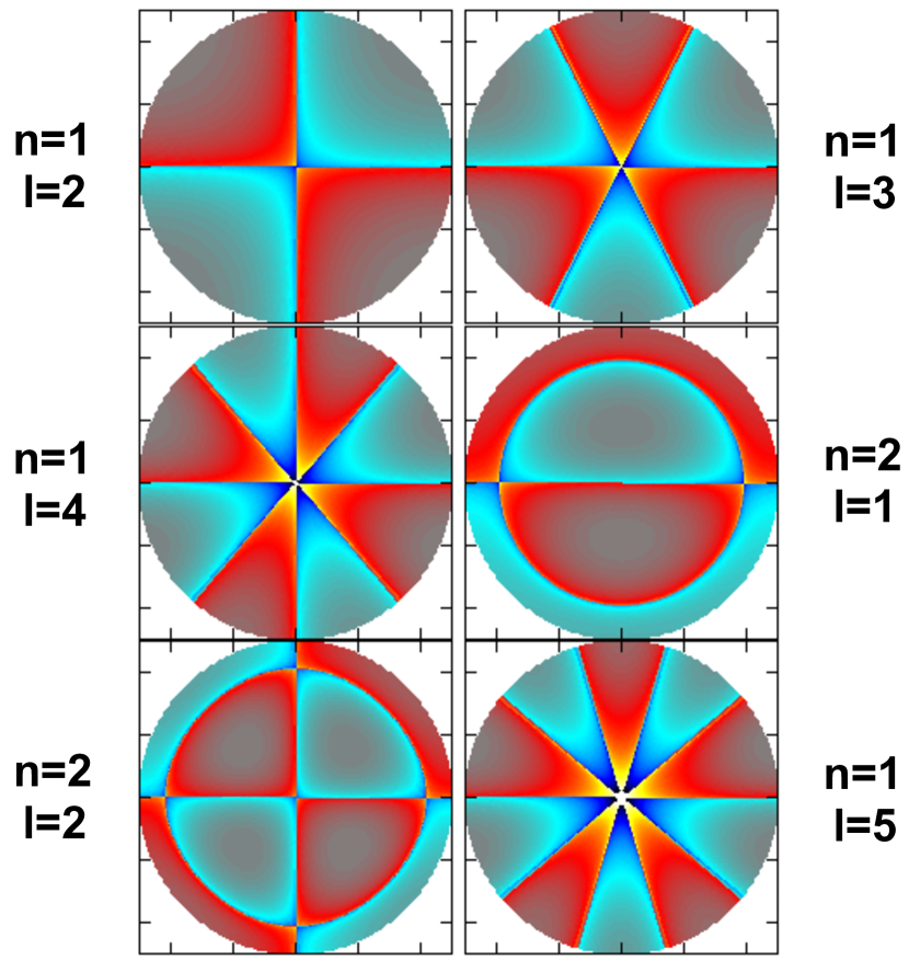
Fig 3: Toroidal vibrational modes. Six different patterns of toroidal vibration at the lowest frequencies in our model of the eye that correspond to the same transversal cut as shown in Fig. 1. Light and dark blue (red and yellow) shades indicated a motion towards (away from) the reader and normal to the drawn plane. Left panels: eigenfunctions with even parity in $l$: ($n=1$, $l=2$) vibrating at 319 Hz, $(1,4)$ at 648 Hz and $(2,2)$ at 909 Hz. Right panels: eigenfunctions with odd parity: $(1,3)$ at 492 Hz, $(2,1)$ at 1159 Hz and $(1,5)$ at 798 Hz.

Table 1: Frequencies of selected normal modes of the eye.

T					S
		$l$					$l$
		1	2	3			1	2	3
$n$	1	734.46	318.71	492.48	$n$	1	2835.9	5706.5	8569.3
	2	1159.0	909.36	1076.1		2	491.41	947.85	1364.7
	3	1570.3	1339.9	1514.1		3	339.58	694.99	1130.0

Left: Table containing the frequencies (measured in Hertz) of selected toroidal modes (T) computed with our numerical code for an average human eyeball. The set of material parameters employed to obtain these values are $R=0.0125$ m, $\rho=1000\,$kg m^-3, $E=0.2985\,$MPa, and $\sigma=0.49$. Toroidal modes with $n=0$ are forbidden since they require driving external forces (assumed non existing in this model). Right: Same as the left table for spheroidal modes (S).

Discussion

In the following, we discuss first the limitations of our current model (Sect. Model limitations). Then, we analyze the prospects to measure the vibrational modes of the eye with existing technologies that where devised for different purposes, but can be suitably adapted (Sect. Methods to measure the eigenfrequencies of the eye).

Model limitations

A more accurate modelling of the eye structure than the one presented in the Sect. Materials and Methods requires differentiating (at least) between the eye interior (including the lens and the aqueous humour) and its elastic boundary (the cornea and the sclera). In our model, this can be done assigning different elastic properties to different parts of the eye. Indeed, it is possible to assign different elastic properties on a point-by-point basis, to account for the heterogeneity of the various eye constituents. The results of such an elaborated model will be published elsewhere. Here, our goal is to outline that the analysis of the normal modes may provide useful mechanical information of the eyeball. If we could measure variations in the eyeball structure and if they could be attributed to normal modes, it would be possible to set an inversion problem [25] to obtain, for instance, the elastic moduli of the eye. The accuracy of the solutions obtained by the inversion problem sensitively depends on the number of properly identified eigenmodes and on the degree of realism in the model of the eyeball. As working hypothesis we assume that variations in the intraocular pressure (IOP) can be used as tracers of the eyeball volumetric changes induced by (spheroidal) normal modes of the eye. A lot of work has been done to connect the dynamics of the intraocular fluid by specifically modelling the aqueous humour as a hydrodynamic system where the inflow/outflow balance of such humour sets its physical properties, including the IOP [26]. The variations of the intraocular blood volume can be produced by many factors, the foremost being pulse, respiration, IOP fluctuations, and nervous mechanisms. The arteries of the eye are thick-walled and relatively inelastic; thus the influence of pulse pressure on intraocular pressure is heavily damped [27]. Contrarily, the venous system is thin-walled and easily collapsible and hence, its volume can sensitively change, though in a tiny amount compared to the full eyeball volume [28]. We also point out that other works have attempted to model only the vitreous humour as a viscoelastic fluid, considering the vitreous chamber as a sphere, and assuming only the effect of toroidal modes (see [29] and references therein). Different from these works, we also compute possible radial modes and present a general method that can be addapted to arbitrary geometries.

Our model needs to be ultimately calibrated with the acquisition of actual data of the eyeball. The ability to measure the changes in the eyeball shape resulting from spheroidal normal modes by mechanical means strongly relies on the maximum amplitude of the deformations induced. In practice, the amplitude of the modes will depend on the amplitude of the perturbations applied to the eye. As we will show in the next section, devices developed for the continuous monitoring of the IOP variations in glaucoma treatment [30] can be used to measure the temporal variations of the eyeball volume (and, thus, its normal modes). Since the inner eye constituents are nearly incompressible, the spherical elastic outer shell comprised of the sclera and the cornea must stretch to accommodate their respective volume changes. The volume of the eyeball may change as a result of the finite compressibility of intraocular tissue (iris, lens, ciliary body) or due to intraocular muscular contraction. However, these latter effects are secondary, and it is primarily the distension of the wall of the eyeball by its incompressible contents that governs the IOP [28].

Methods to measure the eigenfrequencies of the eye

We work under the hypothesis that devices currently employed for the continuous measurement of the IOP or suitable upgrades thereof could be used to measure the eyeball spheroidal normal modes. The idea of measuring the elastic properties of the human eye taking advantage of its internal motions has been treated from different perspectives in the literature. The scattering pattern of attenuated laser sources on the retina has allowed measuring the motion of the vitreous humour [31]. The shear elastic modulus could be determined from these observations [31]. Hence, the same technique can be used to measure toroidal normal modes. The topic has recently gained momentum since the knowledge of the mechanical properties of the vitreous humour is instrumental for finding materials that can be used as vitreous substitutes [1]. Bonfiglio et al. [1] find resonances between the forcing frequency of their device and the artificial vitreous. Remarkably, high frequency resonances may result in undesirably large values of the stress acting on the retina yielding retinal detachments in extreme cases. These resonances are similar to the toroidal eigenmodes we consider here. The frequencies of some of the resonances are above 100 Hz, in line with our results.

Toroidal normal modes of the eye are incompressible and, hence, do not leave a trace on the IOP. The non-invasive character of swept-source optical biometers (SSOBs) is the utmost advantage over alternative techniques for biometric data acquisition [32]. We foresee that the technical capabilities of SSOBs can be improved to obtain high frequency data acquisition of the size of distinct eye structures. Then, they could be used to identify the displacements of the internal constituents of the eye and, therefore, to try to set an inversion problem to recover their normal mode toroidal eigenfrequencies.

Pulse and respiration are periodic phenomena. Therefore, they neither affect the mean IOP nor the eyeball average volume. The typical frequencies of pulse and respiration are below 2 Hz and, thereby, they yield quasi-periodic displacements of the vascular system which can be distinguished from the computed eyeball eigenfrequencies (typically above 100 Hz). Furthermore, in order to trigger the normal eyeball modes, it is optimal to employ perturbations having frequencies as close as possible to the eigenfrequencies. The perturbations induced by pulse and respiration may fall short for this purpose if the (non-linear) mode coupling is weak. Micro saccadic motions of the eye can potentially trigger normal modes, since they happen at frequencies of up to $\sim 60\,$Hz, typically last $20-200$ ms and their rotational peak speeds can be as large as 1000 deg/sec [33]. Micro saccades follow the saccadic main sequence, suggesting a common generator for micro saccades and saccades [33]. Micro saccadic motions are triggered by oscillatory motions of suitable frequencies [34]. The lowest frequencies of the normal modes of our model are close to the observed micro saccadic frequencies, or even closer to measured tremors, which consist of very fast ($\sim 90\,$Hz), extremely small oscillation (about the diameter of a foveal cone) superimposed on drifts [33].

There are intraocular sensors that require surgical implantation, e.g., telemetric pressure transducer systems [35], which have an acquisition rate of $\sim 500\,$Hz, which may suffice for the purpose of measuring the lowest frequency spheroidal modes in a human eye. So far, the high-frequency IOP fluctuations have been attributed to measurement noise [35]. Yet, our results suggest the possibility that they are (partly) produced by the eyeball eigenfrequencies.

Among the least invasive devices to monitor the IOP soft contact lens sensors [36] (CLS) seem to be promising for our purposes. The CLS measure at rates of 10 Hz. This acquisition rate is insufficient to detect the volume variations induced by spheroidal modes. Likely, faster measurement rates are technically plausible. However, such ability is possibly not employed because there was no reason to provide a finer coverage of the IOP variations so far. Should it be technically viable to improve the data acquisition rate in CLS based devices, they could be used for the purpose of measuring the eye’s normal mode eigenfrequencies.

Since toroidal normal modes are incompressible, they may not be registered by the continuous monitoring of the IOP. However, toroidal normal modes are potentially accessible by alternative devices. The IOLMaster 700 SSOB has shown an excellent performance [37, 38, 39]. Should they take measurements at high enough rate, SSOBs could be used to identify toroidal normal modes. As the later modes yield axial displacements about the eyeball axis, they may produce (tiny) variations of the light propagating in a moving medium [40]. Light rays propagating in a whirling fluid remain straight. The travel times of rays that propagate with or against the flow differ by a characteristic number. The light rays differ by a certain phase. Consequently, light waves that move with or against the medium will show a distinct interference pattern in analogy to the Aharonov-Bohm effect of electrically charged matter waves [41]. Perhaps it will be possible in the near future to employ this effect in optical biometers permitting the measurement of internal displacements of the inner constituents of the eye.

Conclusion

We have presented the first analysis of the normal modes of an idealized human eye to our best knowledge. For that we have imported the analytical results developed in a number of areas of Physics, more precisely in the field of Gravitational Wave Physics.

Finally, we will show that beyond the mechanical characterization of the eyeball components, the normal vibrational modes of the eye could be involved in physiological processes like, e.g., the accommodation.

The normal vibrational modes of the eye could be involved in other physiological processes; e.g., the accommodation. Accommodation occurs through changes in the shape and thickness of the crystalline lens. The thickness and the curvature of the lens increase, causing an increase in the eye’s optical power. Since it is a muscle-induced activity, accommodation is a highly fluctuant and dynamic process. These fluctuations are related to the fluctuations in ocular aberrations, and occur with corresponding frequencies [42, 43, 44]. The microfluctuations of accommodation play an important role in the variability of the optical quality of the eye. There are two main components of the accommodation response: a low frequency component ($<0.5\,$Hz), which corresponds to the drift in the accommodation response, and a peak at higher frequency, in the $1-2\,$Hz band [42, 43]. The vibrational eyeball modes we have considered –having the lowest frequencies– seem to happen on timescales of a few milliseconds. The exact way in which the normal eyeball modes are correlated with the accommodation process is beyond the scope of this paper. However, we anticipate that to tackle such study one would need to improve our current model by, at least, differentiating in the eyeball model the cornea-sclera, the vitreous humour and the lens. Towards this direction we will conduct our future research.

Supporting Information

S1 Appendix.

Analytic normal modes. In linear elasticity, the equation of motion for an homogeneous isotropic elastic solid is given by the Navier-Cauchy equation [24], which can be written either in vector form

$$(\lambda+2\mu)[\nabla(\nabla\cdot\boldsymbol{u})]-\mu[\nabla\times(\nabla\times\boldsymbol{u})]+\boldsymbol{F}=\rho\ddot{\boldsymbol{u}},$$ (14)

or, component-wise, as:

$$\mu\nabla^{2}u_{i}+(\lambda+\mu)\vartheta_{,i}+F_{i}=\rho\ddot{u}_{i},$$ (15)

where $u_{i}$ are the displacements with respect to an equilibrium position, $\vartheta:=\nabla\cdot\boldsymbol{u}$ is the dilatation, double dotted quantities denote the second time derivatives ($\partial_{tt}^{2}$) of such quantities, $\nabla^{2}$ is the Laplacian operator, $F_{i}$ denote the body forces, and $\mu$ and $\lambda$ are the Lamé constants. The Lamé constants are related with the Young’s modulus, $\sigma$, and the Poisson ratio, $E$, by the following expressions:

$$\sigma=\frac{\lambda}{2(\lambda+\mu)},\qquad E=\frac{\mu(3\lambda+2\mu)}{\lambda+\mu}$$ (16)

We start assuming oscillatory solutions of the form

$$u_{i}=u^{\prime}_{i}\cos{(pt+\xi)},$$ (17)

where $p$ is the angular frequency of the perturbation, $u^{\prime}_{i}$ are functions independent of the time $t$ and the constant $\xi$ is independent of the coordinates $x_{i}$ and only modifies the phase of the vibration. Plugging the test solutions Eq. (17) into Eq. (15), one obtains in the absence of body forces ($F_{i}=0$):

$$\mu\Delta u_{i}+(\lambda+\mu)\vartheta_{,i}+\rho p^{2}u_{i}=0,$$ (18)

which can be rewritten in the form of an eigenvalue problem

$$-\frac{\mu}{\rho}\Delta u_{i}-\frac{\lambda+\mu}{\rho}\vartheta_{,i}=p^{2}u_{i}.$$ (19)

where the allowed frequencies of vibration and their corresponding displacements (i.e., distortions of the underlying homogeneous and isotropic structure) correspond to the eigenvalues and eigenvectors of the Navier-Cauchy equation for given boundary conditions (imposed at the eyeball surface; Fig. 1).

There are exact solutions of Eq. (19) for solid elastic bodies in which simple boundary conditions are imposed. One example is a sphere where suitable surface tractions inhibit the momentum through its surface (traction boundary conditions). Under the assumption of axisymmetry and expressing their results in terms of spherical solid harmonics $\omega_{n}$, $\phi_{n+1}$ and $\chi_{n}$, Rue [23] obtained, based on Love [24], analytic solutions for the shapes of these vibrations,

$$u_{i}=\sum_{n}\bigg{[} - \frac{1}{h^{2}}\frac{\partial}{\partial x_{i}}\Big{\{}\omega_{n}\psi_{n}(hr)\Big{\}}+\psi_{n}(\kappa r)\Big{(}\epsilon_{ijk}x_{j}\frac{\partial}{\partial x_{k}}\chi_{n}+\frac{\partial}{\partial x_{i}}\phi_{n+1}\Big{)}$$ (20)

$$- \frac{n+1}{n+2}\psi_{n+2}(\kappa r)\kappa^{2}r^{2n+5}\frac{\partial}{\partial x_{i}}\frac{\phi_{n+1}}{r^{2n+3}}\bigg{]}$$

as well as for the vibrational frequencies of spherical bodies. Here, $\epsilon_{ijk}$ is the Levi-Civita symbol and

$$\psi_{n}(x):=\bigg{(}\frac{1}{x}\frac{\partial}{\partial x}\bigg{)}^{n}\>\frac{\sin x}{x},$$ (21)

In axially symmetric systems, the eigenmodes can be classified in two groups: toroidal and spheroidal. Toroidal modes only involve motion about the symmetry axis sketched in Fig. 1. Toroidal modes are incompressible since they do not change the volume of the eyeball. In this first class of vibrations $\omega_{n}$ and $\phi_{n}$ vanish ($\omega_{n}=\phi_{n}=0$), and the frequency, from which we compute the eigenvalues of the system, is given by:

$$p_{n}=0\quad\mbox{ with }\quad p_{n}:=(n-1)\psi_{n}(\kappa a)+\kappa a\psi^{\prime}_{n}(\kappa a)$$ (22)

Spheroidal modes, implying displacements of the eyeball material in both radial and/or angular directions, are compressible. In this second class of vibrations $\chi_{n}$ vanish ($\chi_{n}=0$). The frequency equation is given by:

$$b_{n}c_{n}-a_{n}d_{n}=0$$ (23)

with:

$$a_{n} := \frac{1}{(2n+1)h^{2}}[\kappa^{2}a^{2}\psi_{n}(ha)+2(n-1)\psi_{n-1}(ha)],$$ (24)

$$b_{n} := -\frac{1}{2n+1}\Big{[}\frac{\kappa^{2}}{h^{2}}\psi_{n}(ha)+\frac{2(n+2)}{ha}\psi^{\prime}_{n}(ha)\Big{]},$$ (25)

$$c_{n} := \kappa^{2}a^{2}\psi_{n}(\kappa a)+2(n-1)\psi_{n-1}(\kappa a),$$ (26)

$$d_{n} := \kappa^{2}\frac{n}{n+1}\Big{[}\psi_{n}(\kappa a)+\frac{2(n+2)}{\kappa a}\psi^{\prime}_{n}(\kappa a)\Big{]}.$$ (27)

S1 Fig.

Three-dimensional representation of the toroidal mode $n=1$ and $l=2$. The mode displayed corresponds to the upper left panel of Fig. 3. The arrows indicate the direction of the motion about the symmetry axis of the system (showed with a black arrow).

References

- 1. Bonfiglio A, Lagazzo A, Repetto R, Stocchino A. An experimental model of vitreous motion induced by eye rotations. Eye and Vision. 2015;2(1):1–10. doi:10.1186/s40662-015-0020-8.
- 2. Uchio E, Ohno S, Kudoh J, Aoki K, Kisielewicz LT. Simulation model of an eyeball based on finite element analysis on a supercomputer. British Journal of Ophthalmology. 1999;83(10):1106–1111. doi:10.1136/bjo.83.10.1106.
- 3. Hugar DL, Ivanisevic A. Materials characterization and mechanobiology of the eye. Materials Science and Engineering: C. 2013;33(4):1867 – 1875. doi:http://dx.doi.org/10.1016/j.msec.2013.02.009.
- 4. Ethier CR, Johnson M, Ruberti J. Ocular Biomechanics and Biotransport. Annual Review of Biomedical Engineering. 2004;6(1):249–273. doi:10.1146/annurev.bioeng.6.040803.140055.
- 5. Morita T, Shoji N, Kamiya K, Fujimura F, Shimizu K. Corneal biomechanical properties in normal-tension glaucoma. Acta Ophthalmologica. 2012;90(1):e48–e53. doi:10.1111/j.1755-3768.2011.02242.x.
- 6. Hirneiß C, Neubauer AS, Yu A, Kampik A, Kernt M. Corneal biomechanics measured with the ocular response analyser in patients with unilateral open-angle glaucoma. Acta Ophthalmologica. 2011;89(2):e189–e192. doi:10.1111/j.1755-3768.2010.02093.x.
- 7. Chung CW, Girard MJA, Jan NJ, Sigal IA. Use and Misuse of Laplace’s Law in OphthalmologyLaplace’s Law in Ophthalmology. Investigative Ophthalmology & Visual Science. 2016;57(1):236. doi:10.1167/iovs.15-18053.
- 8. Jones IL, Warner M, Stevens JD. Mathematical modelling of the elastic properties of retina: A determination of Young’s modulus. Eye. 1992;6(6):556–559.
- 9. H Z, de Guillebon H, J HF. Retinal traction in vitro: biophysical aspects. Invest Ophthalmol. 1972;11:46–55.
- 10. de Guillebon H, H Z. Experimental retinal detachment: biophysical aspects of retinal peeling and stretching. Arch Ophthamol. 1972;87:545–8.
- 11. Lombardo M, Carbone G, Lombardo G, De Santo MP, Barberi R. Analysis of intraocular lens surface adhesiveness by atomic force microscopy. Journal of Cataract & Refractive Surgery. 2009;35(7):1266–1272. doi:10.1016/j.jcrs.2009.02.029.
- 12. Luce D. Determining in vivo biomechanical properties of the cornea with an ocular response analyzer. J Cataract Refract Surg. 2005;31(null):156.
- 13. Terai N, Raiskup F, Haustein M, Pillunat LE, Spoerl E. Identification of Biomechanical Properties of the Cornea: The Ocular Response Analyzer. Current Eye Research. 2012;37(7):553–562. doi:10.3109/02713683.2012.669007.
- 14. Sigal IA, Flanagan JG, Ethier CR. Factors Influencing Optic Nerve Head Biomechanics. Investigative Ophthalmology & Visual Science. 2005;46(11):4189. doi:10.1167/iovs.05-0541.
- 15. Sigal IA, Flanagan JG, Tertinegg I, Ethier CR. Modeling individual-specific human optic nerve head biomechanics. Part II: influence of material properties. Biomechanics and Modeling in Mechanobiology. 2009;8(2):99–109. doi:10.1007/s10237-008-0119-0.
- 16. Lam A, Sambursky RP, Maguire JI. Measurement of Scleral Thickness in Uveal Effusion Syndrome. American Journal of Ophthalmology. 2005;140(2):329–331. doi:10.1016/j.ajo.2005.02.014.
- 17. Oliveira C, Tello C, Liebmann J, Ritch R. Central Corneal Thickness is not Related to Anterior Scleral Thickness or Axial Length. Journal of Glaucoma. 2006;15(3).
- 18. Norman RE, Flanagan JG, Rausch SMK, Sigal IA, Tertinegg I, Eilaghi A, et al. Dimensions of the human sclera: Thickness measurement and regional changes with axial length. Experimental Eye Research. 2010;90(2):277 – 284. doi:http://dx.doi.org/10.1016/j.exer.2009.11.001.
- 19. Vorontsov SV, Christensen-Dalsgaard J, Schou J, Strakhov VN, Thompson MJ. Helioseismic Measurement of Solar Torsional Oscillations. Science. 2002;296(5565):101–103. doi:10.1126/science.1069190.
- 20. Israel GL, Belloni T, Stella L, Rephaeli Y, Gruber DE, Casella P, et al. The Discovery of Rapid X-Ray Oscillations in the Tail of the SGR 1806–20 Hyperflare. The Astrophysical Journal Letters. 2005;628(1):L53.
- 21. Strohmayer TE, Watts AL. Discovery of Fast X-Ray Oscillations during the 1998 Giant Flare from SGR 1900+14. The Astrophysical Journal Letters. 2005;632(2):L111.
- 22. Visscher WM, Migliori A, Bell TM, Reinert RA. On the normal modes of free vibration of inhomogeneous and anisotropic elastic objects. The Journal of the Acoustical Society of America. 1991;90(4):2154–2162. doi:http://dx.doi.org/10.1121/1.401643.
- 23. Rue J. On the Normal Modes of Freely Vibrating Elastic Objects of Various Shapes [Master thesis]. University of Amsterdam. The Netherlands; 1996.
- 24. Love AEH. A Treatise on the Mathematical Theory of Elasticity, 4th Edition. Cambridge University Press; 1944.
- 25. Gough DO, Thompson MJ. The inversion problem. In: Cox AN, Livingston WC, Matthews MS, editors. Solar Interior and Atmosphere; 1991. p. 519–561.
- 26. Lyubimov GA, Moiseeva IN, Stein AA. Dynamics of the intraocular fluid: Mathematical model and its main consequences. Fluid Dynamics. 2007;42(5):684–694. doi:10.1134/S001546280705002X.
- 27. Maurice DM. A Recording Tonometer. The British Journal of Ophthalmology. 1958;42(6):321–335.
- 28. Weinbaum S. A mathematical model for the elastic and fluid mechanical behavior of the human eye. The bulletin of mathematical biophysics. 1965;27(3):325–354. doi:10.1007/BF02478410.
- 29. Meskauskas J, Repetto R, Siggers JH. Oscillatory motion of a viscoelastic fluid within a spherical cavity. Journal of Fluid Mechanics. 2011;685:1–22. doi:10.1017/jfm.2011.263.
- 30. Mansouri K. The Road Ahead to Continuous 24-Hour Intraocular Pressure Monitoring in Glaucoma. Journal of Ophthalmic & Vision Research. 2014;9(2):260–268.
- 31. Zimmerman RL. In vivo measurements of the viscoelasticity of the human vitreous humor. Biophysical Journal. 1980;29(3):539 – 544. doi:http://dx.doi.org/10.1016/S0006-3495(80)85152-6.
- 32. Srivannaboon S, Chirapapaisan C, Chonpimai P, Loket S. Clinical comparison of a new swept-source optical coherence tomography–based optical biometer and a time-domain optical coherence tomography–based optical biometer. Journal of Cataract & Refractive Surgery. 2015;41(10):2224 – 2232. doi:http://dx.doi.org/10.1016/j.jcrs.2015.03.019.
- 33. Martinez-Conde S, Macknik SL, Troncoso XG, Hubel DH. Microsaccades: a neurophysiological analysis. Trends in Neurosciences. 2009;32(9):463 – 475. doi:http://dx.doi.org/10.1016/j.tins.2009.05.006.
- 34. Tian X, Yoshida M, Hafed ZM. A Microsaccadic Account of Attentional Capture and Inhibition of Return in Posner Cueing. Frontiers in Systems Neuroscience. 2016;10(23). doi:10.3389/fnsys.2016.00023.
- 35. Downs JC, Burgoyne CF, Seigfreid WP, Reynaud JF, Strouthidis NG, Sallee V. 24-Hour IOP Telemetry in the Nonhuman Primate: Implant System Performance and Initial Characterization of IOP at Multiple Timescales. Investigative Ophthalmology & Visual Science. 2011;52(10):7365. doi:10.1167/iovs.11-7955.
- 36. Leonardi M, Pitchon EM, Bertsch A, Renaud P, Mermoud A. Wireless contact lens sensor for intraocular pressure monitoring: assessment on enucleated pig eyes. Acta Ophthalmologica. 2009;87(4):433–437. doi:10.1111/j.1755-3768.2008.01404.x.
- 37. Kunert KS, Peter M, Blum M, Haigis W, Sekundo W, Schütze J, et al. Repeatability and agreement in optical biometry of a new swept-source optical coherence tomography–based biometer versus partial coherence interferometry and optical low-coherence reflectometry. Journal of Cataract & Refractive Surgery. 2016;42(1):76 – 83. doi:http://dx.doi.org/10.1016/j.jcrs.2015.07.039.
- 38. Akman A, Asena L, Güngör SG. Evaluation and comparison of the new swept source OCT-based IOLMaster 700 with the IOLMaster 500. British Journal of Ophthalmology. 2015;doi:10.1136/bjophthalmol-2015-307779.
- 39. Ferrer-Blasco T, Esteve-Taboada JJ, Monsálvez-Romín D, Aloy MA, Adsuara JE, Cerdá-Durán P, et al. Ocular biometric changes with different accommodative stimuli using swept-source optical coherence tomography. Graefes Archive for Clinical and Experimental Ophthalmology (in press). 2016;.
- 40. Leonhardt U, Piwnicki P. Optics of nonuniformly moving media. Phys Rev A. 1999;60:4301–4312. doi:10.1103/PhysRevA.60.4301.
- 41. Aharonov Y, Bohm D. Significance of Electromagnetic Potentials in the Quantum Theory. Phys Rev. 1959;115:485–491. doi:10.1103/PhysRev.115.485.
- 42. Campbell FW, Robson JG, Westheimer G. Fluctuations of accommodation under steady viewing conditions. The Journal of Physiology. 1959;145(3):579–594.
- 43. Charman WN, Heron G. Fluctuations in accommodation: a review. Ophthalmic and Physiological Optics. 1988;8(2):153–164. doi:10.1111/j.1475-1313.1988.tb01031.x.
- 44. Dubra A. A Shearing Interferometer for the Evaluation of Human Tear Film Topography [Ph.D. Thesis]. Imperial College. London; 2004.