All-optical signatures of Strong-Field QED in the vacuum emission picture

Abstract

We study all-optical signatures of the effective nonlinear couplings among electromagnetic fields in the quantum vacuum, using the collision of two focused high-intensity laser pulses as an example. The experimental signatures of quantum vacuum nonlinearities are encoded in signal photons, whose kinematic and polarization properties differ from the photons constituting the macroscopic laser fields. We implement an efficient numerical algorithm allowing for the theoretical investigation of such signatures in realistic field configurations accessible in experiment. This algorithm is based on a vacuum emission scheme and can readily be adapted to the collision of more laser beams or further involved field configurations. We solve the case of two colliding pulses in full 3+1 dimensional spacetime, and identify experimental geometries and parameter regimes with improved signal-to-noise ratios.

I Introduction

The fluctuations of virtual particles in the quantum vacuum gives rise to effective interactions among electromagnetic fields, supplementing Maxwell’s linear theory of vacuum electrodynamics with effective nonlinearities Heisenberg:1935qt ; Weisskopf ; Schwinger:1951nm ; for reviews, see Refs. Dittrich:1985yb ; Dittrich:2000zu ; Marklund:2008gj ; Dunne:2008kc ; Heinzl:2008an ; DiPiazza:2011tq ; Dunne:2012vv ; Battesti:2012hf ; King:2015tba ; Karbstein:2016hlj . Prominent signatures of quantum vacuum nonlinearities are vacuum magnetic birefringence (VMB) Toll:1952 ; Baier and direct light-by-light scattering Euler:1935zz ; Karplus:1950zza .

Being of quantum nature, the latter are typically tiny and rather elusive in experiment. In quantum electrodynamics (QED), they are suppressed parametrically with inverse powers of the electron mass $m_{e}$. This mass scale serves as the typical energy to be compared with the scales of the applied fields, and defines the critical field strengths $E_{\text{cr}}:=\frac{c^{3}}{\hbar}\frac{m_{e}^{2}}{e}\approx 1.3\times 10^{16}\frac{\rm V}{\rm cm}$ and $B_{\text{cr}}:=\frac{E_{\text{cr}}}{c}\approx 4\times 10^{9}{\rm T}$.

In the laboratory, field strengths of this order are only reached in strong Coulomb fields of highly charged ions. Hence, experimental verifications of QED vacuum nonlinearities have so far been limited to high-energy experiments with highly charged ions Lee:1998hu ; Akhmadaliev:1998zz ; Akhmadaliev:2001ik ; dEnterria:2013zqi ; Aaboud:2017bwk . Note, that VMB is potentially also relevant for the optical polarimetry of neutron stars Mignani:2016fwz ; Capparelli:2017mlv ; Turolla:2017tqt . Even though QED vacuum nonlinearities in macroscopic electromagnetic fields have not been directly verified yet, laboratory searches of VMB in macroscopic magnetic fields Cantatore:2008zz ; Berceau:2011zz ; Fan:2017fnd have already demonstrated the need for high field strengths and, at the same time, a high signal detection sensitivity, see also Zavattini:2016sqz ; Inada:2017 . The demand for strong fields together with the recent technological advances in the development of high-intensity laser systems have opened up an alternative route to access the extreme-field territory in the laboratory. The overarching key idea is to combine high-intensity lasers with polarization sensitive single photon detection schemes.

State-of-the-art high-intensity lasers reach peak field strengths of the order of $10^{6}{\rm T}$ and $10^{12}{\rm V}/{\rm cm}$ in micron sized focal spots. Laser pulses achieving these field strengths are typically made up of ${\cal O}(10^{20})$ photons, constituting a challenging background for the detection of the generically tiny signals of QED vacuum nonlinearities in experiment. In this context, theoretical proposals specifically focused on VMB Heinzl:2006xc ; DiPiazza:2006pr ; Dinu:2013gaa ; Karbstein:2015xra ; Schlenvoigt:2016 ; Karbstein:2016lby ; King:2016jnl ; Bragin:2017yau , photon-photon scattering in the form of laser-pulse collisions Lundstrom:2005za ; Lundin:2006wu ; King:2012aw , quantum reflection Gies:2013yxa ; Gies:2014wsa , photon merging Yakovlev:1966 ; DiPiazza:2007cu ; Gies:2014jia ; Gies:2016czm and splitting Adler:1970gg ; BialynickaBirula:1970vy ; Adler:1971wn ; Papanyan:1971cv ; DiPiazza:2007yx , and optical signatures of QED vacuum nonlinearities based on interference effects King:2013am ; Tommasini:2010fb ; Hatsagortsyan:2011 .

In this article, we introduce and benchmark an efficient numerical algorithm tailored to the study of all-optical signatures of QED vacuum nonlinearities. Reformulating the signatures in terms of vacuum emission processes Karbstein:2014fva , the effects of quantum vacuum nonlinearities are encoded in signal photons emitted from the strong-field region. As no signal photons are induced in the absence of vacuum nonlinearities, these photons generically constitute a distinct signal. However, in order to allow for their detection in experiment, they have to differ from the photons constituting the high-intensity laser pulses driving the effects, e.g., by their kinematic and polarization properties. Correspondingly, one central objective is to identify scenarios where such effects are most pronounced.

A standard approach of dealing with this challenge is to solve the nonlinear photon wave equation, i.e. a partial differential equation, by suitable numerical techniques. Successful examples can be found, e.g., in King:2012aw , where the nonlinearities of the field equations have been treated as source terms and Green’s function methods are used for an iterative solution strategy; see also King:2014vha ; Bohl:2015uba for an advanced implementation based on the pseudo-characteristic method of lines. For large-scale simulation purposes, an implicit ODE-based solver has been specifically designed in Domenech:2016xx , as well as in Carneiro:2016qus using a finite-difference time-domain solver.

As demonstrated in the following, the vacuum emission picture advocated in this work is particularly suited for a numerical implementation. In our formalism, the essential numerical ingredients are reduced to one standard and easy-to-use algorithm: fast Fourier transformation. Space- or time-integrated observables may additionally require simple low-dimensional integration techniques. This numerical simplicity parallels the conceptual adaption of the vacuum emission scheme to the physical situation: in this picture, all macroscopically controlled fields such as high-intensity laser pulses are treated as classical fields, whereas the fluctuation-induced signal photons are dealt with on the level of the quantum Fock space.

Our article is organized as follows: In Sec. II we outline the theoretical foundations of our approach. We apply our methods in Sec. III to the collision of two focused, linearly polarized high-intensity laser pulses in vacuum King:2012aw . In Sec. IV, we introduce our numerical algorithm in detail. Section V is devoted to the discussion of explicit results. Here, we first benchmark our numerical algorithm with analytical results for the limit of infinite Rayleigh ranges of the two beams, where analytical results are available. Subsequently, we use it to obtain new results: in Sec. V.1, we study the collision of two petawatt class laser pulses of identical frequency, continuing with fundamental and doubled frequency in Sec. V.2. Considering the fundamental frequency laser beam as focused down to the diffraction limit, the latter scenario allows for the study of two limiting cases of specific interest, differing in the focusing of the frequency-doubled beam. In the first case, it is focused to the diffraction limit of the fundamental frequency beam, maximizing the beam overlap in the focus, and in the second case to its own diffraction limit, resulting in a narrower beam waist and thus in a considerably smaller overlap region of the beams but higher intensity in the focus. Finally, we end with conclusions and an outlook in Sec. VI.

II Theoretical foundations

In Ref. Karbstein:2014fva , it has been argued that all-optical signatures of quantum vacuum nonlinearities can be efficiently analyzed by reformulating them in terms of vacuum emission processes. This approach has meanwhile been successfully employed to obtain experimentally realistic predictions for the phenomenon of VMB, particularly in the combination of x-ray free electron and high-intensity lasers Karbstein:2015xra ; Karbstein:2015qwa ; Karbstein:2016lby .

The central idea is to consider all applied macroscopic electromagnetic fields as constituting the external background field; cf also Ref. Gies:2016yaa . This implies, that the quantum character of the applied fields is not resolved, and effects like, e.g., QED-induced beam depletion are neglected. We emphasize that this is typically well-justified for scenarios where the strong electromagnetic fields $E$ and $B$ are provided by high-intensity lasers and fulfill $E\ll E_{\text{cr}}$ and $B\ll B_{\text{cr}}$. Due to the parametric suppression of QED vacuum nonlinearities by powers of the electron mass, the pulses delivered by such lasers can be considered as traversing each other in vacuum essentially unaltered.

At one-loop order, but fully nonperturbative in the background field $\bar{A}$, the exact interaction term giving rise to single signal photon emission is given by Gies:2016yaa

$$\Gamma_{\text{int}}^{(1)}[\bar{A}(x)]=\int{\rm d}^{4}x\,\frac{\delta\Gamma^{1\text{-loop}}_{\text{HE}}[A]}{\delta A^{\mu}}\bigg{|}_{A=\bar{A}(x)}a^{\mu}(x)\,,$$ (1)

where $\Gamma^{1\text{-loop}}_{\text{HE}}[A]=-{\rm i}\ln\det(-{\rm i}\not{\partial}-e\not{A}+m_{e})$ is the one-loop Heisenberg-Euler action evaluated in the generic external field $A\equiv A(x)$. Our metric convention is $g_{\mu\nu}=\mathrm{diag}(-1,+1,+1,+1)$, and we use the Heaviside-Lorentz System with $c=\hbar=1$.

In turn, the amplitude for emission of a single signal photon with momentum $\vec{k}$ from the QED vacuum subject to the external field $\bar{A}$ is given by Karbstein:2014fva (cf. also Fig. 1)

$${\cal S}_{(p)}(\vec{k})\equiv\big{\langle}\gamma_{p}(\vec{k})\big{|}\Gamma_{\text{int}}^{(1)}[\bar{A}(x)]\big{|}0\big{\rangle}\,.$$ (2)

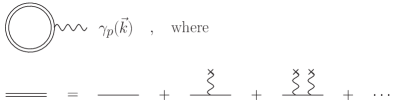
Figure 1: Diagrammatic representation of the single photon vacuum emission process (2). The double line denotes the dressed fermion propagator accounting for arbitrarily many couplings to the external field $\bar{A}$, represented by the wiggly lines ending at crosses.

Here $|\gamma_{p}(\vec{k})\rangle\equiv a^{\dagger}_{\vec{k},p}|0\rangle$ denotes the single signal photon state, and $p$ labels the polarization of the emitted photons. Transition amplitudes to final states with more photons can be constructed along the same lines, but are typically suppressed because of a significantly larger phase space for the signal photons; cf. the photon splitting process in Ref. Gies:2016czm . The differential number of signal photons with polarization $p$ to be measured far outside the interaction region is then given by

$${\rm d}^{3}N_{(p)}(\vec{k})=\frac{{\rm d}^{3}k}{(2\pi)^{3}}\bigl{|}{\cal S}_{(p)}(\vec{k})\bigr{|}^{2}\,.$$ (3)

Representing the photon field in Lorenz gauge as

$$a^{\mu}(x) =\sum_{p}\int\frac{{\rm d}^{3}{k}}{(2\pi)^{3}}\frac{1}{\sqrt{2k^{0}}}$$

$$\quad\quad\times\Bigl{(}\epsilon^{\mu}_{(p)}(k)\,{\rm e}^{-{\rm i}kx}\,a_{\vec{k},p}+\epsilon^{*\mu}_{(p)}(k)\,{\rm e}^{{\rm i}kx}a^{\dagger}_{\vec{k},p}\Bigl{)},$$ (4)

where $k^{0}\equiv|\vec{k}|$, $kx:=k^{\mu}x_{\mu}$ and the sum is over the two physical (transverse) photon polarizations, Eq. (2) can be expressed as

$${\cal S}_{(p)}(\vec{k})=\frac{\epsilon^{*\mu}_{(p)}(k)}{\sqrt{2k^{0}}}\int{\rm d}^{4}x\,{\rm e}^{{\rm i}kx}\,\frac{\delta\Gamma^{1\text{-loop}}_{\text{HE}}[A]}{\delta A^{\mu}}\bigg{|}_{A=\bar{A}(x)}.$$ (5)

No closed-form expressions of Eq. (5) for generic background field profiles are available. For the field configurations generated by high-intensity lasers, which vary on length (time) scales much larger than the Compton wavelength (time) of the electron $\lambdabar_{\rm C}\approx 3.86\cdot 10^{-13}{\rm m}$ ($\tau_{\rm C}\approx 1.29\cdot 10^{-21}{\rm s}$), analytical insights are nevertheless possible by means of a locally constant field approximation (LCFA).

The LCFA amounts to first obtaining the Heisenberg-Euler action in constant electromagnetic fields, $\bar{F}^{\mu\nu}=\partial^{\mu}\bar{A}^{\nu}-\partial^{\nu}\bar{A}^{\mu}=\text{const.}$, resulting in a closed-form expression $\Gamma_{\text{HE}}(\bar{F})$. As already determined in the original works Heisenberg:1935qt ; Schwinger:1951nm , $\Gamma_{\text{HE}}(\bar{F})$ is a function of the two field invariants ${\cal F}=\frac{1}{4}\bar{F}_{\mu\nu}\bar{F}^{\mu\nu}=\frac{1}{2}(\vec{B}^{2}-\vec{E}^{2})$ and ${\cal G}=\frac{1}{4}\bar{F}_{\mu\nu}{}^{*}\bar{F}^{\mu\nu}=-\vec{B}\cdot\vec{E}$, where ${}^{*}\bar{F}^{\mu\nu}=\frac{1}{2}\epsilon^{\mu\nu\alpha\beta}\bar{F}_{\alpha\beta}$. Adopting this result for inhomogeneous fields, yields the LCFA approximation for the action functional,

$$\Gamma_{\text{HE}}(\bar{F})=\int{\rm d}^{4}x\,{\cal L}_{\text{HE}}(\bar{F})\quad\\ \xrightarrow{\bar{F}\to\bar{F}(x)}\quad\Gamma_{\text{HE}}\bigl{[}\bar{F}(x)\bigr{]}=\int{\rm d}^{4}x\,{\cal L}_{\text{HE}}\bigl{(}\bar{F}(x)\bigr{)}.$$ (6)

Due to parity invariance of QED, the dependency of the Heisenberg-Euler Lagrangian is actually even in $\cal G$, such that ${\cal L}_{\text{HE}}\bigl{(}\bar{F})={\cal L}_{\text{HE}}\bigl{(}{\cal F},{\cal G}^{2})$ for constant fields as well as for the LCFA. As has been argued, e.g., in Refs. Galtsov:1982 ; Karbstein:2015cpa ; Gies:2016yaa , the deviations of the LCFA result from the corresponding exact expression for $\Gamma_{\text{HE}}$ are of order ${\cal O}\bigl{(}(\tfrac{\upsilon}{m_{e}})^{2}\bigr{)}$, where $\upsilon$ delimits the moduli of the frequency and momentum components of the considered inhomogeneous field from above.

Within the LCFA, we obtain Karbstein:2014fva ; Karbstein:2015cpa ; Gies:2016yaa

$${\cal S}_{(p)}(\vec{k})={\rm i}\frac{\epsilon^{*\mu}_{(p)}(k)}{\sqrt{2k^{0}}}\,\int{\rm d}^{4}x\,{\rm e}^{{\rm i}kx}\,\\ \times\biggl{[}(k\bar{F})_{\mu}\frac{\partial{\cal L}_{\text{HE}}^{1\text{-loop}}}{\partial{\cal F}}+(k\,{}^{*}\!\bar{F})_{\mu}\frac{\partial{\cal L}_{\text{HE}}^{1\text{-loop}}}{\partial{\cal G}}\biggr{]},$$ (7)

where $(k\bar{F})_{\mu}:=k^{\nu}\bar{F}_{\nu\mu}(x)$, $(k\,{}^{*}\!\bar{F})_{\mu}:=k^{\nu}\,{}^{*}\!\bar{F}_{\nu\mu}(x)$ and

$$\frac{\partial{\cal L}_{\text{HE}}^{1\text{-loop}}}{\partial{\cal F}}=\frac{\alpha}{2\pi}\int_{0}^{\infty}\frac{{\rm d}s}{s}\,{\rm e}^{-{\rm i}\frac{m_{e}^{2}}{e}s}\\ \qquad\ \times\biggl{[}\frac{ab}{a^{2}+b^{2}}\frac{as\cot(bs)}{\sinh^{2}(as)}+(a\leftrightarrow{\rm i}b)+\frac{2}{3}\biggr{]},$$ (8)

$$\frac{\partial{\cal L}_{\text{HE}}^{1\text{-loop}}}{\partial{\cal G}}=\frac{\alpha}{2\pi}\int_{0}^{\infty}\frac{{\rm d}s}{s}\,{\rm e}^{-{\rm i}\frac{m_{e}^{2}}{e}s}\,{\cal G}\,\coth(as)\cot(bs)\\ \times\biggl{[}\frac{1}{2ab}-\frac{1}{a^{2}+b^{2}}\frac{bs}{\sinh(as)\cosh(as)}+(a\leftrightarrow{\rm i}b)\biggr{]},$$ (9)

with $a:=(\sqrt{{\cal F}^{2}(x)+{\cal G}^{2}(x)}-{\cal F}(x))^{1/2}$ and $b:=(\sqrt{{\cal F}^{2}(x)+{\cal G}^{2}(x)}+{\cal F}(x))^{1/2}$.

Using spherical momentum coordinates $\vec{k}={\rm k}\hat{\vec{k}}$, where ${\rm k}=\sqrt{k_{\rm x}^{2}+k_{\rm y}^{2}+k_{\rm z}^{2}}$ and $\hat{\vec{k}}=(\cos\varphi\sin\vartheta,\sin\varphi\sin\vartheta,\cos\vartheta)$, the vectors perpendicular to $\vec{k}$ can be parameterized by a single angle $\beta$,

$$\hat{\vec{e}}_{\beta}=\left(\begin{array}[]{c}\cos\varphi\cos\vartheta\cos\beta-\sin\varphi\sin\beta\\ \sin\varphi\cos\vartheta\cos\beta+\cos\varphi\sin\beta\\ -\sin\vartheta\cos\beta\end{array}\right).$$ (10)

Correspondingly, the transverse polarization modes of photons with wave vector $\vec{k}$ can be spanned by two orthonormalized four-vectors, e.g.,

$$\epsilon^{\mu}_{(1)}(\vec{k}):=(0,\hat{\vec{e}}_{\beta})\quad\textrm{and}\quad\epsilon^{\mu}_{(2)}(\vec{k}):=(0,\hat{\vec{e}}_{\beta+\frac{\pi}{2}})\,,$$ (11)

for a suitable choice of $\beta$. With these definitions, we obtain

$${\cal S}_{(1)}(\vec{k}) =\frac{1}{{\rm i}}\sqrt{\frac{k^{0}}{2}}\int{\rm d}^{4}x\,{\rm e}^{{\rm i}kx}$$

$$\quad\times\biggl{\{}\bigl{[}\hat{\vec{e}}_{\beta}\cdot\vec{E}(x)-\hat{\vec{e}}_{\beta+\frac{\pi}{2}}\cdot\vec{B}(x)\bigr{]}\frac{\partial{\cal L}_{\text{HE}}^{1\text{-loop}}}{\partial{\cal F}}$$

$$\quad\ \ \,+\bigl{[}\hat{\vec{e}}_{\beta}\cdot\vec{B}(x)+\hat{\vec{e}}_{\beta+\frac{\pi}{2}}\cdot\vec{E}(x)\bigr{]}\frac{\partial{\cal L}_{\text{HE}}^{1\text{-loop}}}{\partial{\cal G}}\biggr{\}}$$ (12)

and ${\cal S}_{(2)}(\vec{k})={\cal S}_{(1)}(\vec{k})\big{|}_{\beta\to\beta+\frac{\pi}{2}}$, using $\hat{\vec{e}}_{\beta+\pi}=-\hat{\vec{e}}_{\beta}$. In the limit of weak electromagnetic fields, $e\bar{F}^{\mu\nu}\ll m_{e}^{2}$, Eq. (9) results in

$$\left\{\begin{array}[]{c}\dfrac{\partial{\cal L}_{\text{HE}}^{1\text{-loop}}}{\partial{\cal F}}\\[8.61108pt] \dfrac{\partial{\cal L}_{\text{HE}}^{1\text{-loop}}}{\partial{\cal G}}\end{array}\right\}=\frac{\alpha}{\pi}\frac{1}{45}\Bigl{(}\frac{e}{m_{e}^{2}}\Bigr{)}^{2}\left\{\begin{array}[]{c}4{\cal F}(x)\\[4.30554pt] 7{\cal G}(x)\end{array}\right\}+{\cal O}\bigl{(}(\tfrac{e\bar{F}}{m_{e}^{2}})^{4}\bigr{)}\,,$$ (13)

such that Eq. (12) becomes

$${\cal S}_{(1)}(\vec{k})= \frac{1}{{\rm i}}\frac{e}{4\pi^{2}}\frac{m_{e}^{2}}{45}\sqrt{\frac{k^{0}}{2}}\Bigl{(}\frac{e}{m_{e}^{2}}\Bigr{)}^{3}\int{\rm d}^{4}x\,{\rm e}^{{\rm i}kx}$$

$$\times\Bigl{\{}\,4\bigl{[}\hat{\vec{e}}_{\beta}\cdot\vec{E}(x)-\hat{\vec{e}}_{\beta+\frac{\pi}{2}}\cdot\vec{B}(x)\bigr{]}{\cal F}(x)$$

$$\quad+7\bigl{[}\hat{\vec{e}}_{\beta}\cdot\vec{B}(x)+\hat{\vec{e}}_{\beta+\frac{\pi}{2}}\cdot\vec{E}(x)\bigr{]}{\cal G}(x)\Bigr{\}}\,,$$ (14)

where we neglected higher-order terms of ${\cal O}\bigl{(}(\frac{e\bar{F}}{m_{e}^{2}})^{5}\bigr{)}$. The corresponding Feynman diagram is depicted in Fig. 2.

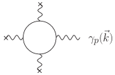
Figure 2: Leading contribution to the single photon vacuum emission process in the limit of weak external fields.

Because of Furry’s theorem, in QED the total number of couplings of fermion loops to electromagnetic fields (i.e., including the signal photon) is always even. For single signal photon emission, the number of couplings to the external field is odd.

In spherical coordinates, the differential number of signal photons of Eq. (3) can finally be expressed as

$${\rm d}^{3}N_{(p)}(\vec{k})={\rm dk}\,{\rm d}\varphi\,{\rm d}\!\cos\vartheta\,\frac{1}{(2\pi)^{3}}\bigl{|}{\rm k}{\cal S}_{(p)}(\vec{k})\bigr{|}^{2}\,.$$ (15)

Moreover, it is convenient to introduce the total number density of induced signal photons polarized in mode $p$ and emitted in the direction ($\varphi$, $\vartheta$) as follows Karbstein:2014fva ,

$$\rho_{(p)}(\varphi,\vartheta):=\frac{1}{(2\pi)^{3}}\int_{0}^{\infty}{\rm dk}\,\bigl{|}{\rm k}{\cal S}_{(p)}(\vec{k})\bigr{|}^{2}\,.$$ (16)

The total number of signal photons of polarization $p$ is then obtained as $N_{(p)}:=\int_{0}^{2\pi}{\rm d}\varphi\int_{-1}^{1}{\rm d}\!\cos\vartheta\,\rho_{(p)}(\varphi,\vartheta)$. Accordingly, the total number of signal photons of any polarization is given by $N:=\sum_{p=1}^{2}N_{(p)}$, and the associated number density by $\rho:=\sum_{p=1}^{2}\rho_{(p)}$.

III Collision of two high-intensity laser pulses

In the present work, we consider the collision of two high-intensity laser pulses as a concrete example for our computational scheme. On the one hand, this configuration already features a high degree of complexity due to a substantial set of experimentally tunable laser and geometry parameters. On the other hand, this case is sufficiently simple to allow for analytically or semi-analytically insights which are essential for reliably benchmarking our numerical procedure.

Let us thus assume the background electric and magnetic fields to be generated by the superposition of two linearly polarized laser beams. In leading-order paraxial approximation, each of these laser beams is characterized by a single, globally fixed wave vector and its electric and magnetic fields. We define the normalized wave vectors of the two laser beams $b\in\{1,2\}$ as $\hat{\kappa}_{b}^{\mu}=(1,\hat{\vec{e}}_{\kappa_{b}})$. The associated electric and magnetic fields are characterized by an overall amplitude profile ${\cal E}_{b}$ and point in $\hat{\vec{e}}_{E_{b}}$ and $\hat{\vec{e}}_{B_{b}}$ directions. These unit vectors are independent of $x$ for linear polarization. They fulfill $\hat{\vec{e}}_{E_{b}}\cdot\hat{\vec{e}}_{B_{b}}=\hat{\vec{e}}_{E_{b}}\cdot\hat{\vec{e}}_{\kappa_{b}}=\hat{\vec{e}}_{B_{b}}\cdot\hat{\vec{e}}_{\kappa_{b}}=0$ and $\hat{\vec{e}}_{E_{b}}\times\hat{\vec{e}}_{B_{b}}=\hat{\vec{e}}_{\kappa_{b}}$. Hence, in this case Eq. (14) can be expressed as

$${\cal S}_{(1)}(\vec{k})=\frac{1}{{\rm i}}\frac{e}{4\pi^{2}}\frac{m_{e}^{2}}{45}\sqrt{\frac{k^{0}}{2}}\Bigl{(}\frac{e}{m_{e}^{2}}\Bigr{)}^{3}\int{\rm d}^{4}x\,{\rm e}^{{\rm i}kx}\,{\cal E}_{1}^{2}(x){\cal E}_{2}(x)$$

$$\quad\times\Bigl{[}4\bigl{(}\hat{\vec{e}}_{\beta}\cdot\hat{\vec{e}}_{E_{1}}-\hat{\vec{e}}_{\beta+\frac{\pi}{2}}\cdot\hat{\vec{e}}_{B_{1}}\bigr{)}\bigl{(}\hat{\vec{e}}_{B_{1}}\cdot\hat{\vec{e}}_{B_{2}}-\hat{\vec{e}}_{E_{1}}\cdot\hat{\vec{e}}_{E_{2}}\bigr{)}$$

$$\quad\,\ -7\bigl{(}\hat{\vec{e}}_{\beta}\cdot\hat{\vec{e}}_{B_{1}}+\hat{\vec{e}}_{\beta+\frac{\pi}{2}}\cdot\hat{\vec{e}}_{E_{1}}\bigr{)}\bigl{(}\hat{\vec{e}}_{B_{1}}\cdot\hat{\vec{e}}_{E_{2}}+\hat{\vec{e}}_{E_{1}}\cdot\hat{\vec{e}}_{B_{2}}\bigr{)}\Bigr{]}$$

$$\quad\quad\quad\quad+({\cal E}_{1}\leftrightarrow{\cal E}_{2},\hat{\vec{e}}_{B_{1}}\leftrightarrow\hat{\vec{e}}_{B_{2}},\hat{\vec{e}}_{E_{1}}\leftrightarrow\hat{\vec{e}}_{E_{2}})\,.$$ (17)

The generalization of Eq. (17) to background fields generated by more laser beams is straightforward. Without loss of generality we assume the beam axes of the two lasers to be confined to the xz-plane and parameterize the unit wave and field vectors as

$$\hat{\vec{e}}_{\kappa_{b}} =\left(\begin{array}[]{c}\sin\vartheta_{b}\\ 0\\ \cos\vartheta_{b}\end{array}\right),\quad\hat{\vec{e}}_{E_{b}} =\left(\begin{array}[]{c}\cos\vartheta_{b}\cos\beta_{b}\\ \sin\beta_{b}\\ -\sin\vartheta_{b}\cos\beta_{b}\end{array}\right),$$ (24)

and $\hat{\vec{e}}_{B_{b}}=\hat{\vec{e}}_{E_{b}}\big{|}_{\beta_{b}\to\beta_{b}+\frac{\pi}{2}}$, where the choice of $\beta_{b}$ fixes the polarization of the beam. Throughout this article, we assume $\vartheta_{1}=0$, such that the first laser beam propagates along the positive $\rm z$ axis. In turn, the angle $\vartheta_{2}$ parameterizes the tilt of the beam axis of the second laser beam with respect to the first. With these definitions, the terms written explicitly in Eq. (17) can be expressed as

$${\cal S}_{(1)}(\vec{k})={\rm i}\frac{\sqrt{\alpha}}{(2\pi)^{3/2}}\frac{m_{e}^{2}}{45}\Bigl{(}\frac{e}{m_{e}^{2}}\Bigr{)}^{3}(1-\cos\vartheta_{2})\sqrt{\rm k}$$

$$\times\biggl{\{}{\cal I}_{21}(k)(1-\cos\vartheta)f(\beta_{1}+\beta_{2},\beta+\beta_{1}-\varphi)$$

$$\quad+{\cal I}_{12}(k)\Bigl{[}\bigl{[}(1-\cos\vartheta\cos\vartheta_{2})\cos\varphi-\sin\vartheta\sin\vartheta_{2}\bigr{]}$$

$$\hskip 85.35826pt\times f(\beta_{1}+\beta_{2},\beta+\beta_{2})$$

$$\quad\quad-\sin\varphi(\cos\vartheta-\cos\vartheta_{2})\,g(\beta_{1}+\beta_{2},\beta+\beta_{2})\Bigl{]}\biggr{\}}\,,$$ (25)

where we have made use of the shorthand notations

$$\begin{split}f(\mu,\nu)&:=4\cos\mu\cos\nu+7\sin\mu\sin\nu\,,\\ g(\mu,\nu)&:=4\cos\mu\sin\nu-7\sin\mu\cos\nu\,,\end{split}$$ (26)

and

$${\cal I}_{mn}(k):=\int{\rm d}^{4}x\,{\rm e}^{{\rm i}{\rm k}(\hat{\vec{k}}\cdot\vec{x}-t)}\,{\cal E}_{1}^{m}(x){\cal E}_{2}^{n}(x)\,.$$ (27)

Hence, the only remaining nontrivial task in determining the single photon emission amplitude is to compute the Fourier transforms (27). As it is linear in ${\cal E}_{1}$ (${\cal E}_{2}$), the contribution $\sim{\cal I}_{12}$ ($\sim{\cal I}_{21}$) in Eq. (25) can, for instance, be interpreted as signal photons originating from the laser beam characterized by the field profile ${\cal E}_{1}$ (${\cal E}_{2}$), which are scattered into a different kinematic and polarization mode due to interactions with the other laser beam described by ${\cal E}_{2}$ (${\cal E}_{1}$).

In a next step we specify the amplitude profiles ${\cal E}_{b}$ of the two laser beams, which we assume to be well-described by pulsed Gaussian laser beams of the following amplitude profile (cf., e.g., Refs. Siegman ; Karbstein:2015cpa )

$${\cal E}_{b}(x)={\cal E}_{0,b}\,{\rm e}^{-\frac{({\rm z}_{b}-t_{b})^{2}}{(\tau_{b}/2)^{2}}}\frac{w_{0,b}}{w_{b}({\rm z}_{b})}\,{\rm e}^{-\frac{r_{b}^{2}}{w_{b}^{2}({\rm z})}}\\ \times\cos\Bigl{(}\omega_{b}({\rm z_{b}}-t_{b})+\tfrac{{\rm z}_{b}}{{\rm z}_{R,b}}\tfrac{r_{b}^{2}}{w_{b}^{2}({\rm z}_{b})}-\arctan\tfrac{{\rm z}_{b}}{{\rm z}_{R,b}}+\varphi_{0,b}\Bigr{)}\,,$$ (28)

with ${\rm z}_{b}:=\hat{\vec{e}}_{\kappa_{b}}\cdot(\vec{x}-\vec{x}_{0,b})$, $t_{b}:=t-t_{0,b}$ and $r_{b}:=\sqrt{(\vec{x}-\vec{x}_{0,b})^{2}-{\rm z}_{b}^{2}}$. Here, ${\cal E}_{0,b}$ is the peak field strength, $\omega_{b}=\frac{2\pi}{\lambda_{b}}$ the photon energy and $\tau_{b}$ the pulse duration. The beam is focused at $\vec{x}=\vec{x}_{0,b}$, where the peak field is reached for $t=t_{0,b}$. Its waist size is $w_{0,b}$ and its Rayleigh range is ${\rm z}_{R,b}=\pi w_{0,b}^{2}/\lambda_{b}$. The widening of the beam’s transverse extent as a function of ${\rm z}_{b}$ is encoded in the function $w_{b}({\rm z}_{b})=w_{0,b}\sqrt{1+({\rm z}_{b}/{\rm z}_{R,b})^{2}}$, $\arctan\bigl{(}\tfrac{{\rm z}_{b}}{{\rm z}_{R,b}}\bigr{)}$ is the Gouy phase of the beam and $\varphi_{0,b}$ determines its phase in the focus. The total angular spread $\Theta_{b}$ and the radial beam divergence $\theta_{b}$ far from the beam waist are given by $\Theta_{b}=2\,\theta_{b}\simeq 2\,\frac{w_{0,b}}{{\rm z}_{R,b}}$.

Without loss of generality, in the remainder of this article we will assume $x_{0,1}^{\mu}=(0,\vec{0})$, such that the temporal and spatial offsets of the two beams are fully controlled by $x_{0,2}^{\mu}=:(t_{0},\vec{x}_{0})$.

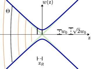
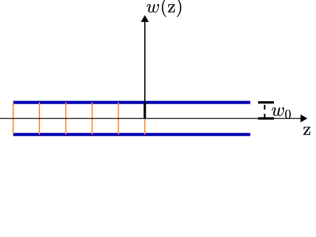
Figure 3: Sketch of the transverse field amplitude profile of a generic Gaussian beam (left) and the special case of a Gaussian beam with infinite Rayleigh range, but finite beam waist (right) as a function of the longitudinal coordinate (measured along the propagation axis). Here, $\Theta$ is the total angular spread, $w_{0}$ is the beam waist and ${\rm z}_{R}$ is the Rayleigh range over which the beam diameter increases by a factor of $\sqrt{2}$.

With regard to the Fourier integrals (27), it is particularly helpful to note that the $m$-th power of the field profile (28) can be expressed as

$${\cal E}_{b}^{m}(x) =\Bigl{(}\frac{{\cal E}_{0,b}}{2}\Bigr{)}^{m}\sum_{l=0}^{m}\binom{m}{l}c_{b;lm}({\rm z}_{b},r_{b})$$

$$\quad\times{\rm e}^{{\rm i}(m-2l)[\omega_{b}({\rm z}_{b}-t_{b})+\varphi_{0,b}]}\,{\rm e}^{-4m\left({\rm z}_{b}-t_{b}\right)^{2}/\tau_{b}^{2}},$$ (29)

where

$$c_{b;lm}({\rm z}_{b},r_{b})=\frac{{\rm e}^{-(\nicefrac{{r_{b}}}{{w_{0,b}}})^{2}\,[\frac{m-l}{1+{\rm i}\frac{{\rm z}_{b}}{{\rm z}_{R,b}}}+\frac{l}{1-{\rm i}\frac{{\rm z}_{b}}{{\rm z}_{R,b}}}]}}{(1+{\rm i}\frac{{\rm z}_{b}}{{\rm z}_{R,b}})^{m-l}\,(1-{\rm i}\frac{{\rm z}_{b}}{{\rm z}_{R,b}})^{l}}\,,$$ (30)

which can be derived straightforwardly from Eq. (22) of Ref. Karbstein:2015cpa by employing the binomial theorem. Note that the entire dependence of Eq. (29) on the Rayleigh range ${\rm z}_{R,b}$ and the transverse structure of the laser fields is encoded in the function $c_{b;lm}({\rm z}_{b},r_{b})$.

The integration over time in Eq. (27) can be easily performed analytically for generic values of ${\rm z}_{R,b}$, resulting in

$${\cal I}_{mn}(k)=\Bigl{(}\frac{{\cal E}_{0,1}}{2}\Bigr{)}^{m}\Bigl{(}\frac{{\cal E}_{0,2}}{2}\Bigr{)}^{n}\frac{\sqrt{\pi}}{2}\frac{\tau_{1}\tau_{2}}{\sqrt{m\tau_{2}^{2}+n\tau_{1}^{2}}}$$

$$\quad\times\sum_{l=0}^{m}\sum_{j=0}^{n}\binom{m}{l}\binom{n}{j}\int{\rm d}^{3}x\,{\rm e}^{{\rm i}{\rm k}(\hat{\vec{k}}\cdot\vec{x})}\,$$

$$\quad\times c_{1;lm}({\rm z}_{1},r_{1})\,c_{2;jn}({\rm z}_{2},r_{2})\,{\rm e}^{-4[m(\frac{{\rm z}_{1}}{\tau_{1}})^{2}+n(\frac{{\rm z}_{2}+t_{0}}{\tau_{2}})^{2}]}$$

$$\quad\times{\rm e}^{-\frac{\left\{{\rm k}+(m-2l)\omega_{1}+(n-2j)\omega_{2}+8{\rm i}[m{\rm z}_{1}/\tau_{1}^{2}+n({\rm z}_{2}+t_{0})/\tau_{2}^{2}]\right\}^{2}}{16(m/\tau_{1}^{2}+n/\tau_{2}^{2})}}$$

$$\quad\times{\rm e}^{{\rm i}\left\{(m-2l)(\omega_{1}{\rm z}_{1}+\varphi_{0,1})+(n-2j)[\omega_{2}({\rm z}_{2}+t_{0})+\varphi_{0,2}]\right\}}\,.$$ (31)

Let us now briefly focus on the limit of infinitely long pulse durations, $\{\tau_{1},\tau_{2}\}\to\infty$. To this end, we first set $\tau_{2}=\tau_{1}$ and subsequently send $\tau_{1}\to\infty$. This results in the following expression,

$$\lim_{\{\tau_{1},\tau_{2}\}\to\infty}{\cal I}_{mn}(k)=\delta\bigl{(}{\rm k}+(m-2l)\omega_{1}+(n-2j)\omega_{2}\bigr{)}$$

$$\quad\quad\times 2\pi\,\Bigl{(}\frac{{\cal E}_{0,1}}{2}\Bigr{)}^{m}\Bigl{(}\frac{{\cal E}_{0,2}}{2}\Bigr{)}^{n}\sum_{l=0}^{m}\sum_{j=0}^{n}\binom{m}{l}\binom{n}{j}$$

$$\quad\quad\times\int{\rm d}^{3}x\,{\rm e}^{{\rm i}{\rm k}(\hat{\vec{k}}\cdot\vec{x})}\,c_{1;lm}({\rm z}_{1},r_{1})\,c_{2;jn}({\rm z}_{2},r_{2})$$

$$\quad\quad\quad\times{\rm e}^{{\rm i}\left\{(m-2l)(\omega_{1}{\rm z}_{1}+\varphi_{0,1})+(n-2j)[\omega_{2}({\rm z}_{2}+t_{0})+\varphi_{0,2}]\right\}}$$

$$\quad\quad\quad\times{\rm e}^{-{\rm i}\frac{[(m-2l)\omega_{1}+(n-2j)\omega_{2}+{\rm k}][m{\rm z}_{1}+n({\rm z}_{2}+t_{0})]}{m+n}},$$ (32)

where we have employed the identity $\lim_{\tau\to\infty}\tau\,{\rm e}^{-\frac{\tau^{2}}{2}\chi^{2}}=\sqrt{2\pi}\,\delta(\chi)$. The argument of the Dirac delta function in Eq. (32) reflects the various possibilities of energy transfer from the laser beams to the signal photons. Due to the strictly harmonic time dependences of the beams in the limit $\{\tau_{1},\tau_{2}\}\to\infty$, implying sharp laser photon energies $\{\omega_{1},\omega_{2}\}$, only signal photons with sharp energies ${\rm k}$ are induced; recall that $\{\omega_{1},\omega_{2},{\rm k}\}\geq 0$. Hence, particularly for $\{\tau_{1},\tau_{2}\}\to\infty$, the ${\cal I}_{nm}(k)$ in Eq. (25) generically give rise to signal photons of energy

$${\rm k}=\begin{cases}\omega_{1}\\ \omega_{1}+2\omega_{2}\\ \lvert\omega_{1}-2\omega_{2}\rvert\\ \omega_{2}\\ \omega_{2}+2\omega_{1}\\ \lvert\omega_{2}-2\omega_{1}\rvert\end{cases}.$$ (33)

For finite pulse durations the time dependences of the beams are no longer purely harmonic, and correspondingly the signal frequencies in general no longer sharp and discrete, but rather smeared and continuous. However, for pulse durations fulfilling $\{\omega_{1}\tau_{1},\omega_{2}\tau_{2}\}\gg 1$, the signal frequencies should still be strongly peaked around the values listed in Eq. (33).

In the limit of infinite Rayleigh ranges $\{{\rm z}_{R,1},{\rm z}_{R,2}\}\to\infty$, also the spatial Fourier integral in Eq. (31) can be performed analytically; cf. also Ref. Karbstein:2016lby . For this, we note that

$$c_{b;lm}({\rm z}_{b},r_{b})\,\xrightarrow{{\rm z}_{R,b}\to\infty}\,{\rm e}^{-(\nicefrac{{r_{b}}}{{w_{0,b}}})^{2}\,m}\,.$$ (34)

Physically, the latter limit is only justified for weakly focused laser beams, as it automatically implies $w_{0,b}\gg\lambda_{b}$; see the definition of ${\rm z}_{R,b}$ in terms of $w_{0,b}$ and $\lambda_{b}$ given above. In the following, we use the limit (34) as an estimate also for values of $w_{0,b}/\lambda_{b}={\cal O}(1)$, serving below as a toy model benchmark test for the numerical method. This ad-hoc looking toy-model approximation can still be justified by the following observation: The emission of signal photons from the QED vacuum becomes substantial only in the overlap region of the focused high-intensity laser pulses where the electromagnetic fields become maximal. In particular for collisions with vanishing offset of the laser foci, the approximation based on Eq. (34) is expected to reproduce the essential quantitative features of the experimental signal. For an illustration of the beam profiles used, see Fig. 3.

IV Numerical implementation

The vacuum emission amplitude, carrying all information about the asymptotic signal photon, can in principle be straightforwardly evaluated for any given external field. To the present one-loop order within the LCFA, we may start with Eq. (7), or to leading-order with Eq. (14), corresponding to a 4-dimensional Fourier transformation from spacetime to energy-momentum space.

In the present work, we continue to use the paraxial laser beam shapes as an illustration. Generalizations to arbitrary spacetime-dependent fields are straightforward on the basis of a 4-dimensional fast Fourier transform (FFT). For the laser pulses under consideration, we take advantage of the Gaussian time structure as in Eq. (28). Then, the Fourier transformation in time can be performed analytically, leaving us with a 3-dimensional space integration (as, e.g., in Eq. (31)). Reducing the integration domain, for instance, to a cubic box, the control parameters for a numerical integration are, e.g., the size parameter of the box $L_{\text{x}},L_{\text{y}},L_{\text{z}},$ and the number of grid points in each direction $N_{\text{x}},N_{\text{y}},N_{\text{z}}$.

The lengths $L_{i}$ have to be chosen large enough to enclose the interaction region where the focused fields are strong. A natural choice is a few times the laser focus size parameters, see App. A for more details. The number of grid points is slightly more subtle: first, this number must be high enough to resolve the pulse structure at a sub-cycle level. Second, the grid must also be sufficiently fine to resolve the momentum structure of the outgoing signal photon. In the case of sum-frequency generation as in Eq. (33), it is this momentum scale of the signal photons which governs the grid resolution parameters $N_{i}$. Throughout this article we use a grid size of $512\times 256\times 512$.

Whereas the 4-dimensional integration in Eq. (7) corresponds to a Fourier transform, the reduced 3-dimensional case in Eq. (31) strictly speaking does not from the viewpoint of an FFT algorithm, as the integrand also depends on the signal photon energy ${\rm k}=\sqrt{k_{\rm x}^{2}+k_{\rm y}^{2}+k_{\rm z}^{2}}$. In practice, this is not problematic, as the integral can still be treated as a numerical Fourier transform upon insertion of a set of fiducial energies ${\rm k}_{u}$, $u=0,1,\dots,N_{\Delta({\rm k})}$ into the integrand. For a given ${\rm k}_{u}$, the 3-dimensional integral is again a Fourier transform to $k_{\rm x,y,z}$ space which we perform via FFT. The physical result then satisfies the constraint ${\rm k}_{u}\overset{!}{=}\sqrt{k_{\rm x}^{2}+k_{\rm y}^{2}+k_{\rm z}^{2}}$. In practice, this implies that we also need to choose a grid in fiducial ${\rm k}_{u}$ space parametrized by a size of ${\rm k}$-grid intervals $\Delta({\rm k})$ and the number $N_{\Delta({\rm k})}$ of intervals. In the present case of colliding laser pulses, this discretization is straightforward to choose as the peak locations are known from energy conservation a la Eq. (33), and the peak width being inversely proportional to the pulse durations. The necessity of introducing a fiducial momentum grid ${\rm k}_{u}$ renders the numerical problem 4-dimensional again. Nevertheless, the advantage is that the spatial grid requires $N_{\text{x,y,z}}=\mathcal{O}(100-1000)$, whereas $N_{\Delta({\rm k})}=\mathcal{O}(10)$ is sufficient for the present problem.

Concentrating on the case of colliding laser pulses as outlined above, we observe that the spatial and directional properties of the laser fields factorize in the general emission rate (17). Thus, it is beneficial to decompose the calculation scheme into three individual steps: (i) calculation of the Fourier integrals ${\cal I}_{mn}$, (ii) evaluation of the factors in Eq. (25) encoding the lasers’ polarization and collision geometry and (iii) determination of the directional emission characteristics of the signal photons. This specific design allows for building highly flexible code enabling, e.g., efficient parallelization. For the sake of convenience, we have summarized the scheme in Proc. 1.

As the present collision set-up has a well-defined scattering center, it is useful to characterize the signal photon in spherical momentum coordinates $({\rm k},\varphi,\vartheta)$ rather than in Cartesian coordinates $\left(k_{\rm x},\,k_{\rm y},\,k_{\rm z}\right)$. Hence, step (i) does not only involve the FFT to $k_{\rm x,y,z}$ space, but also a mapping to a polar and azimuthal angle grid discretized into $N_{\vartheta}$ and $N_{\varphi}$ intervals, respectively. The radial momentum is already fixed by the constraint ${\rm k}=\sqrt{\vphantom{\sum}k_{\rm x}^{2}+k_{\rm y}^{2}+k_{\rm z}^{2}}$. This mapping is sketched in Fig. 4.

Procedure 1 Pseudocode showing the general evaluation routine. The blocks are called consecutively, taking as input arguments only the results from the previous task.

Code:

Initialization

for all ${\rm k}_{u}$ do

     for all ${\cal I}_{mn}$ do

         Fourier transform from $\left({\rm x},{\rm y},{\rm z}\right)$ to $\left(k_{\rm x},k_{\rm y},k_{\rm z}\right)$

         Map from $\left(k_{\rm x},k_{\rm y},k_{\rm z}\right)$ to $\left(\varphi\,,\vartheta\right)$

     end for

end for

for all $\varphi_{v}\,,\vartheta_{w}$ do

     Specify the polarization $\beta$ of the signal photons

     Calculate emission rates $\mathcal{S}_{\beta}$, $\rho_{\beta}$

end for

Post processing

Notation:
${\rm x},\,{\rm y},\,{\rm z},\,k_{\rm x},\,k_{\rm y},\,k_{\rm z},\,\varphi,\,\vartheta$	discrete variables
${\rm k}_{u}$, $\varphi_{v}$, $\vartheta_{w}$	index denotes the loop variable
$\left(\ldots\right)$	denotes a domain

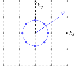
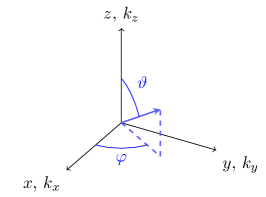
Figure 4: Top: Sketch of the mapping from a regular grid ($k_{x}$, $k_{y}$) to a polar grid with fixed radius ($\varphi$). Light gray (dark blue) nodes represent the discretization in Cartesian coordinates (polar coordinates) in momentum space. As gray and blue nodes generally do not overlap, we apply cubic interpolation. Bottom: Sketch of the coordinate systems used. Spatial as well as momentum coordinates are originally given in Cartesian coordinate systems. In spherical coordinates the angles $\varphi$ and $\vartheta$ give the longitude and latitude ($\vartheta\in\left[0,\pi\right]$), respectively. In our numerical calculation only regular grids were used.

Upon combination with the functions encoding the collision geometry and the polarization properties of the driving laser fields in Eq. (25), it is straightforward to obtain the discretized version of the differential number of signal photons with energy ${\rm k}_{u}$, emitted in the direction $(\varphi_{v},\vartheta_{w})$ from Eq. (3), where $u=0,\dots N_{\Delta({\rm k})},v=1,\dots,N_{\varphi},w=1,\dots,N_{\vartheta}$. Throughout this article we use $N_{\Delta({\rm k})}=31$, $N_{\varphi}=257$ and $N_{\vartheta}=513$. Note, that at this point the polarization properties of the signal photons have to be specified.

The discretized version of the directional emission rate (16) is obtained by summing over all ${\rm k}_{u}$ and is given by

$$\rho_{(p)}(\varphi,\vartheta) \approx\rho_{(p)}(\varphi_{v},\vartheta_{w})$$

$$=\frac{1}{(2\pi)^{3}}\sum_{u=0}^{N_{\Delta({\rm k})}}W_{{\rm k}_{u}}\,|{\rm k}_{u}\,\mathcal{S}_{(p)}({\rm k}_{u},\vartheta_{v},\varphi_{w})|^{2},$$ (35)

where $W_{{\rm k}_{u}}$ denotes a weight function that is specified by the integration algorithm. Already simple integration routines give a good rate of convergence. For maximum simplicity, we hence apply the trapezoidal rule, resulting in

$$\rho_{(p)}(\varphi_{v},\vartheta_{w})=\frac{1}{(2\pi)^{3}}\frac{{\rm k}_{N_{\Delta({\rm k})}}-{\rm k}_{0}}{2N_{\Delta({\rm k})}}\Biggl{[}|{\rm k}_{0}\,\mathcal{S}_{(p)}({\rm k}_{0})|^{2}\phantom{\sum_{0}^{1}}\\ +2\sum_{u=1}^{N_{\Delta({\rm k})}-1}|{\rm k}_{u}\,\mathcal{S}_{(p)}({\rm k}_{u})|^{2}+|{\rm k}_{N_{\Delta({\rm k})}}\,\mathcal{S}_{(p)}({\rm k}_{N_{\Delta({\rm k})}})|^{2}\Biggr{]}.$$ (36)

The total number of signal photons polarized in mode $p$ is then approximately given by

$$N_{(p)}\approx\sum_{v=0}^{N_{\varphi}}W_{\varphi_{v}}\sum_{w=0}^{N_{\vartheta}}W_{\vartheta_{w}}\sin\left(\vartheta_{w}\right)\rho_{(p)}\left(\varphi_{v},\vartheta_{w}\right),$$ (37)

with weights $W_{\varphi_{v}}$ and $W_{\vartheta_{w}}$. Similarly to Eq. (35), even simple routines provide a good rate of convergence. Hence, the trapezoidal rule is used again as the simplest method.

V Results

In the following, we provide explicit results for the prospective numbers of signal photons attainable in the collision of two high-intensity laser pulses characterized by the field profiles introduced in Sec. III. More specifically, we consider two identical lasers of the one petawatt (PW) class, delivering pulses of duration $\tau=25{\rm fs}$ and energy $W=25{\rm J}$ at a wavelength of $\lambda=800{\rm nm}$ (photon energy $\omega=\frac{2\pi}{\lambda}\approx 1.55{\rm eV}$). The peak intensity of a given laser pulse in the focus is then given by Karbstein:2017jgh

$$I_{0,b}={\cal E}_{0,b}^{2}\approx 8\sqrt{\frac{2}{\pi}}\frac{W}{\pi w_{0,b}^{2}\tau}\,.$$ (38)

As the effects of QED vacuum nonlinearities become more pronounced for higher field strengths, we aim at minimizing the beam waists $w_{0,b}$ of the driving laser beams to maximize their peak field strengths. The minimum value of the beam waist $w_{0,b}$ is obtained when focusing the Gaussian beam down to the diffraction limit. The actual limit is given by $w_{0,b}=\lambda_{b}f^{\#}$, where $f^{\#}$ is the so-called $f$-number, defined as the ratio of the focal length and the diameter of the focusing aperture Siegman ; $f$-numbers as low as $f^{\#}=1$ can be realized experimentally. Being particularly interested in the maximum number of signal photons, we mainly consider the case of an optimal overlap of the colliding laser pulses and set the offset parameters $x_{0,2}^{\mu}=(t_{0},\vec{x}_{0})$ to zero. Furthermore, in the remainder of this article we assume the two lasers to be polarized perpendicularly to the collision plane, corresponding to the choice of $\beta_{1}=\beta_{2}=\frac{\pi}{2}$, and to deliver pulses of the same pulse duration, $\tau_{1}=\tau_{2}=\tau$.

V.1 Collision of laser pulses of identical frequency

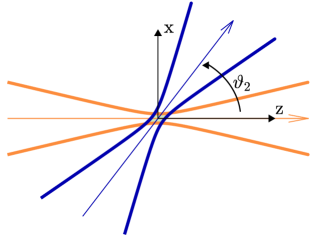
Figure 5: Sketch of the collision geometry considered in Sec. V.1. Two Gaussian laser pulses collide under an angle $\vartheta_{2}$ with respect to their beam axes; the offset between the beam foci is $\vec{x}_{0}=0$. Note that an angle of $\vartheta_{2}=0^{\circ}$($180^{\circ}$) corresponds to co(counter)-propagating laser beams.

In a first step, we adopt the choice of $\omega_{1}=\omega_{2}=\frac{2\pi}{\lambda}$ and assume that both lasers are focused down to the diffraction limit with $f^{\#}=1$. Correspondingly, we have $w_{0,1}=w_{0,2}=\lambda$. For a sketch of the considered collision geometry, see Fig. 5. Note that the specific scenario considered here is reminiscent of the one studied in Ref. Karbstein:2014fva . However, here we go substantially beyond this initial study, which only focused on exactly counter propagating beams and resorted to various additional simplifications, grasping only the most elementary features of Gaussian laser beams.

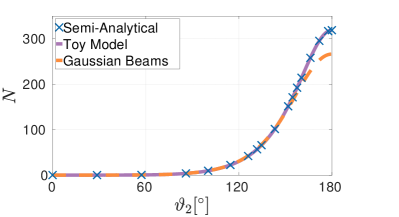
Figure 6: Total number of signal photons $N$ attainable per shot in the collision of two identical high-intensity laser pulses ($w_{0,1}=w_{0,2}=\lambda=800$nm, $W=25$J, $\tau=25$fs) plotted as a function of the collision angle $\vartheta_{2}$. The dashed line shows the results for the advanced description of the colliding laser fields in terms of pulsed Gaussian beams, evaluated numerically with our algorithm. In addition, we present results for the toy-model benchmark scenario of keeping $w_{0,1}=w_{0,2}=\lambda$ finite but formally sending ${\rm z}_{R,b}\to\infty$. The latter scenario is analyzed in two different ways: By means of a fully numerical calculation with our algorithm (solid line), and by performing the Fourier transform from position to momentum space analytically, and numerically integrating over the outgoing signal photon momenta with Maple^TM (cross symbols).

Table 1: Benchmark calculations for the total numbers of signal photons attainable in the toy model scenario with $w_{0,1}=w_{0,2}=\lambda$ finite, but ${\rm z}_{R,b}\to\infty$; see also Figs. 6 and 8. The good agreement of the results confirms the excellent performance of our numerical code. We only state the mean relative error for the total numbers of signal photons $\text{MRE}_{N}$, as these numbers generally show the largest deviation.

	(a) Numerical		(b) Semi-analytical		Mean relative error
$\vartheta_{2}[{}^{\circ}]$	$N$	$N_{\perp}$	$N$	$N_{\perp}$	$\text{MRE}_{N}[\%]$
90	5.03	0.33	5.04	0.33	0.2
135	69.40	0.59	69.43	0.60	0.04
180	330.19	0.15	330.24	0.15	0.02

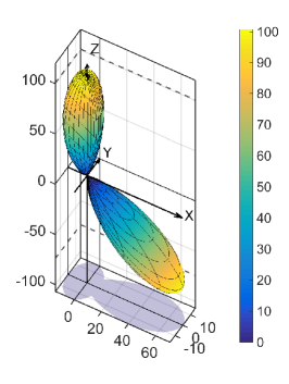
Figure 7: Directional emission characteristics of signal photons for two identical laser pulses colliding under an angle of $\vartheta_{2}=135{}^{\circ}$. Top: Three-dimensional plot of the total number density $\rho(\varphi,\vartheta)$. For illustration, we also include a projection of the emission characteristics onto the xy-plane (gray). Bottom: Projection of the directional emission characteristics (top) onto the collision plane of the laser pulses (xz-plane). For comparison, the forward cones of the colliding Gaussian laser beams with $f^{\#}=1$ and delimited by the beams’ divergences $\theta_{b}=\frac{1}{\pi}$ representing the background are highlighted in gray.

Figure 6 shows the total number of signal photons $N$ as a function of the collision angle $\vartheta_{2}$. Here, we depict the results for pulsed Gaussian beams with Rayleigh ranges ${\rm z}_{R,b}$ given self-consistently by ${\rm z}_{R,b}=(\pi w_{0,b}^{2})/\lambda=\pi\lambda$ (dashed line). We also compare it to the toy-model benchmark scenario, where ${\rm z}_{R,b}$ is treated as an independent parameter, which is formally sent to infinity; cf. Sec. III above. This figure also demonstrates that the results obtained with our numerical algorithm (solid line) for the toy-model scenario with ${\rm z}_{R,b}\to\infty$ are in satisfactory agreement with benchmark data points (cross symbols). The latter are obtained by performing the Fourier transform from position to momentum space analytically, and the integration over the signal photon momenta numerically using Maple^TM. We infer that the maximum number of signal photons is obtained for a head-on collision of the two high-intensity laser pulses, while no signal photons are induced for co-propagating beams. This fact is well-known from the study of probe photon propagation in constant crossed and plane wave fields; cf., e.g., Ref. Dittrich:2000zu . Even though for collision angles in the range of $120^{\circ}\ldots 180^{\circ}$ signal photon numbers of $N\approx 100$ per shot are attainable, the detection of these photons in experiment would be rather difficult. The reason for this is that these signal photons are predominantly emitted into the forward cones of the incident high intensity lasers. The signal is thus overwhelmed by the background. In Fig. 7 we exemplarily depict the directional emission characteristics for a collision angle of $\vartheta_{2}=135{}^{\circ}$. For comparison, we have depicted the forward cones of the colliding Gaussian laser beams focused down to $f^{\#}=1$ and delimited by the beams’ divergences $\theta_{b}=\frac{1}{\pi}$.

In order to separate a signal – which is detectable at least in principle – from background, we turn to a different observable, namely the fraction of signal photons polarized perpendicularly to the high-intensity laser beams. Due to their distinct polarization, these photons constitute a viable signal that could be extracted with high-purity polarimetry. Recall, that both high-intensity laser beams are polarized perpendicularly to the collision plane ($\beta_{1}=\beta_{2}=\frac{\pi}{2}$).

In Fig. 8 we plot the number of signal photons polarized perpendicularly to the high-intensity laser beams $N_{\perp}$ as a function of $\vartheta_{2}$. For the particular collision scenario considered here, this number follows from the integration of

$$\rho_{\perp}(\varphi,\vartheta):=\frac{1}{(2\pi)^{3}}\int_{0}^{\infty}{\rm dk}\,\bigl{|}{\rm k}{\cal S}_{(1)}(\vec{k})\bigr{|}^{2}\Big{|}_{\beta=-\arctan(\cos\vartheta\tan\varphi)}$$ (39)

over the spherical angles, i.e., $N_{\perp}:=\int_{0}^{2\pi}{\rm d}\varphi\int_{-1}^{1}{\rm d}\!\cos\vartheta\,\rho_{\perp}(\varphi,\vartheta)$. Note that the polarization-angle parameter $\beta$ has to be adjusted as a function of the emission direction $\hat{\vec{k}}$ parameterized by $\{\varphi,\vartheta\}$ in order to project on the perpendicular polarization $\hat{\vec{e}}_{E_{1}}\cdot\hat{\vec{e}}_{\beta}=\hat{\vec{e}}_{E_{2}}\cdot\hat{\vec{e}}_{\beta}=0$ for all $\hat{\vec{k}}$ Karbstein:2016lby . As in Fig. 6, we present results for the collision of pulsed Gaussian laser beams, as well as for the toy model scenario with ${\rm z}_{R,b}\to\infty$. Again the latter scenario is used to benchmark the performance of our numerical algorithm by comparing data points obtained for both strategies.

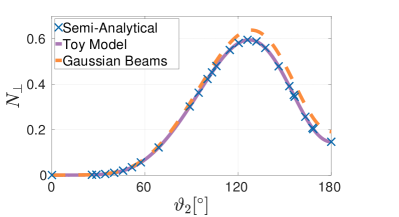
Figure 8: Total number of signal photons polarized perpendicularly to the high-intensity laser beams $N_{\perp}$ plotted as a function of the collision angle $\vartheta_{2}$. Both laser pulses ($w_{0,1}=w_{0,2}=\lambda=800$nm, $W=25$J, $\tau=25$fs) are polarized perpendicularly to the collision plane. The dashed (solid) curve shows the result obtained from a numerical calculation for pulsed Gaussian beams (the benchmark scenario with $w_{0,b}=\lambda$ finite, but ${\rm z}_{R,b}\to\infty$). The cross symbols display data for the benchmark scenario obtained by performing the Fourier transform analytically and evaluating the momentum integral numerically with Maple^TM.

For a more quantitative comparison, we exemplarily list explicit values for the total numbers of attainable signal photons $N$ and $N_{\perp}$ for several collision angles $\vartheta_{2}$ for the benchmark toy-model scenario in Tab. 1. We find a relative difference typically on the order of $\mathcal{O}(0.01\%)$ and maximally of $\sim 0.2\%$ between the semi-analytical approach and our numerical algorithm. While the semi-analytical approach that involves numerical integrations with Maple^TM, we expect these algorithms to have a higher accuracy, also because the integrations are performed over the full (infinite) spacetime volume. The remaining difference hence serves as an error estimate for the numerical algorithm that works with absolute coordinate and momentum space cutoffs due to the nature of the fast Fourier transformation. Concretely, the fast Fourier algorithm treats the integration kernels as if they were periodic functions. We compensate for this by a careful adaptation of the domain of periodicity, such that all relevant information is preserved and no artificial frequencies are introduced. Additionally, the transformation to spherical coordinates as well as the integrations over momentum space in our algorithm come with their discretization errors. A convergence test is illustrated in App. A. In summary, we consider a systematic error of our algorithm below the $1\%$ level and thus possibly below two-loop corrections Dittrich:1998fy as rather satisfactory.

Figure 9: Directional emission characteristics of perpendicularly polarized signal photons for two identical laser pulses colliding under an angle of $\vartheta_{2}=135{}^{\circ}$. Top: Three-dimensional plot of the number density $\rho_{\perp}(\varphi,\vartheta)$. Bottom: Projection of the directional emission characteristics (top) onto the collision plane of the laser pulses (xz-plane). For comparison, the forward cones of the colliding Gaussian laser beams with $f^{\#}=1$ and delimited by the beams’ divergences $\theta_{b}=\frac{1}{\pi}$ are highlighted in gray.

Figure 10: Directional emission characteristics of perpendicularly polarized signal photons for two identical laser pulses colliding under an angle of $\vartheta_{2}=175.8{}^{\circ}$. Top: Three-dimensional plot of the number density $\rho_{\perp}(\varphi,\vartheta)$. For better visibility of the directional emission characteristics, we adopt a perspective different from the other plots. Bottom: Projection of the directional emission characteristics (top) onto the collision plane of the laser pulses (xz-plane). The forward cones of the colliding Gaussian laser beams focused down to $f^{\#}=1$ and delimited by the beams’ divergences $\theta_{b}=\frac{1}{\pi}$ are highlighted in gray.

Coming back to the physics results, Fig. 8 clearly demonstrates that the maximum for perpendicularly polarized signal photons $N_{\perp}$ is shifted to a collision angle of $\vartheta_{2}\approx 120^{\circ}$. Moreover, the perpendicularly polarized signal is significantly smaller than the total one; the maximum number is $N_{\perp}\approx 0.6$. Analogously to Fig. 7, we also provide the directional emission characteristics of the perpendicularly polarized signal for a collision angle of $\vartheta_{2}=135{}^{\circ}$ in Fig. 9.

In addition, we display the analogous emission characteristics for a collision angle of $\vartheta_{2}=175.8{}^{\circ}$ in Fig. 10. Here, the formation of additional pronounced emission peaks opposite to the propagation directions of the high-intensity laser pulses for collision angles $\vartheta_{2}\to 180^{\circ}$ is clearly visible. For a counter-propagation geometry reflection symmetry with respect to the xy-plane is restored Karbstein:2015cpa .

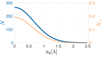
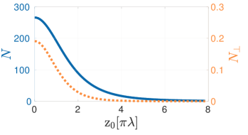
Figure 11: Impact of a relative shift between the laser foci on the integrated numbers of signal photons $N$ (blue solid line, left scale) and $N_{\perp}$ (orange dashed line, right scale) for two identical laser pulses colliding in a counter-propagation geometry, i.e., $\vartheta_{2}=180{}^{\circ}$. Both laser pulses are polarized perpendicularly to the collision plane. Top: Transverse shift with $\vec{x}_{0}=({\rm x}_{0},0,0)$ in units of the waist size $w_{0,1}=w_{0,2}=\lambda$. Bottom: Longitudinal shift along the common beam axis with $\vec{x}_{0}=(0,0,{\rm z}_{0})$ in units of the Rayleigh range ${\rm z}_{R,1}={\rm z}_{R,2}=\pi\lambda$.

Finally, we study the consequences of a spatial displacement $\vec{x}_{0}$ of the laser foci. Because of jitter, such a displacement is generically expected to occur in experiments in a random fashion. For simplicity, we specialize to the head-on collision of two identical high-intensity laser pulses with exactly coinciding beam axes, i.e., $\vartheta_{2}=180{}^{\circ}$, and consider the cases $\vec{x}_{0}=({\rm x}_{0},0,0)$ and $\vec{x}_{0}=(0,0,{\rm z}_{0})$ focused to $w_{0,1}=w_{0,2}=\lambda$. We demonstrate in Fig. 11 how the integrated numbers of signal photons $N$ and $N_{\perp}$ decrease as a function of the relative displacements ${\rm x}_{0}$ and ${\rm z}_{0}$ between the laser foci transverse to or along the common beam axis. For the present case, we observe that the signal photon number $N$ drops by a factor of 2 for ${\rm x}_{0}\approx 0.76\lambda$ and ${\rm z}_{0}\approx 1.5\pi\lambda$.

V.2 Collision of laser pulses of fundamental and doubled frequency

Here we go beyond the scenario considered in the previous section, subsequently referred to as scenario (o). Differently to Sec. V.1, one of the two high-intensity lasers is now assumed to be frequency doubled, such that $\omega_{2}=2\omega_{1}=2\frac{2\pi}{\lambda}$. The energy loss for a frequency-doubling process conserving the pulse duration is estimated conservatively as $50\%$. Correspondingly, we have $\tau_{1}=\tau_{2}=\tau$, $W_{1}=W$ and $W_{2}=W/2$. Keeping the focusing of the fundamental-frequency laser pulse as in the previous section, i.e., $w_{0,1}=\lambda$, we now consider two different scenarios: (i) In order to ensure a maximal spatial overlap of the two laser pulses in their foci, the frequency-doubled laser pulse is focused down to the waist size of the fundamental-frequency laser pulse, i.e., $w_{0,2}=w_{0,1}=\lambda$. This scenario is illustrated in Fig. 12. (ii) For maximizing the peak field strength in the focus, the frequency-doubled pulse is focused down to its diffraction limit with $f^{\#}=1$, resulting in $w_{0,2}=\lambda/2$. This scenario is sketched in Fig. 13.

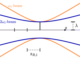
Figure 12: Scenario (i): The two Gaussian beams of fundamental and doubled frequency are focused to a beam waist of $w_{0,1}=w_{0,2}=\lambda$. In this scenario, the beam divergences fulfill $\theta_{2}=\theta_{1}/2$. We depict the case of zero offset, $\vec{x}_{0}=0$, and $\vartheta_{2}\in\{0^{\circ},180^{\circ}\}$.

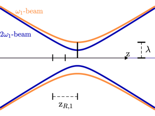
Figure 13: Scenario (ii): The Gaussian beam of fundamental (doubled) frequency is focused to a waist size of $w_{0,1}=\lambda$ ($w_{0,2}=\lambda/2$). In this scenario, the beam divergences fulfill $\theta_{1}=\theta_{2}$. We depict the case of zero offset, $\vec{x}_{0}=0$, and $\vartheta_{2}\in\{0^{\circ},180^{\circ}\}$.

As detailed in Sec. III, for Gaussian beams the Rayleigh range and far-field beam divergence, are intimately related to the wavelength and the waist size. Hence, in case (i) we have ${\rm z}_{R,2}=2{\rm z}_{R,1}$, $\theta_{2}=\theta_{1}/2$, while in case (ii) ${\rm z}_{R,2}={\rm z}_{R,1}/2$, $\theta_{2}=\theta_{1}$; cf. also Figs. 12 and 13. All the results presented in this section are obtained with our algorithm introduced in Sec. IV. In Fig. 14 we show the total number of signal photons $N$ as a function of the collision angle $\vartheta_{2}$ for the cases (o)-(ii).

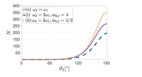
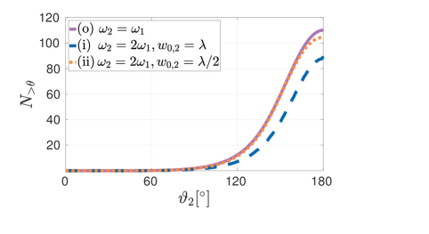
Figure 14: Integrated numbers of signal photons attainable in the various scenarios (o)-(ii) plotted as a function of the collision angle $\vartheta_{2}$. We depict results for (o) the collision of two fundamental frequency laser pulses focused to $w_{0,1}=w_{0,2}=\lambda$, and the collision of fundamental and doubled frequency laser pulses focused to waist sizes (i) $w_{0,2}=w_{0,1}=\lambda$ and (ii) $w_{0,2}=w_{0,1}/2=\lambda/2$. Top: Total number of signal photons $N$. Bottom: Number of signal photons emitted outside the forward cones of the colliding Gaussian laser beams $N_{>\theta}$, delimited by the beams’ radial divergences $\theta_{b}$.

In Sec. III we have argued that the signal photons should predominantly be emitted at several pronounced frequencies if the criterion $\{\omega_{1}\tau,\omega_{2}\tau\}\gg 1$ holds; cf. Eq. (33). For the collision of (o) two fundamental frequency beams we have $\omega_{1}\tau=\omega_{2}\tau\approx 58.9$, while for the cases (i) and (ii), both involving a frequency doubled beam, we have $\{\omega_{1}\tau,\omega_{2}\tau\}\approx\{58.9,117.7\}$.

Hence, as the criterion $\{\omega_{1}\tau,\omega_{2}\tau\}\gg 1$ is obviously fulfilled here, we expect the signal photons to feature primarily frequencies with (o): ${\rm k}\approx\{\omega_{1},3\omega_{1}\}$ and (i), (ii): ${\rm k}\approx\{\omega_{1},2\omega_{1},3\omega_{1},4\omega_{1},5\omega_{1}\}$, respectively. However, inelastic signal photon emission processes are generically suppressed in comparison to the elastic ones. For instance, in Ref. Karbstein:2014fva it was already demonstrated for a simplified model of the head-on collision of fundamental frequency laser pulses that the $3\omega_{1}$ signal is completely negligible in comparison to the $\omega_{1}$ signal. This fully agrees with the results obtained here: In scenario (o) essentially all signal photons are emitted in an energy range $\Delta(\omega_{1})$; here and in the following $\Delta(\omega)$ denotes an interval of photon energies centered around a frequency $\omega$ with an energy width being inversely proportional to the temporal pulse duration. For the scenarios (i) and (ii) we encounter sizable numbers of signal photons in the energy segments $\Delta(\omega_{1})$ and $\Delta(2\omega_{1})$.

Table 2: Prospective numbers of signal photons with energies in the segments $\Delta(\omega_{1})$ and $\Delta(2\omega_{1})$ for the example of a collision angle of $\vartheta_{2}=135^{\circ}$. Both high-intensity laser pulses are polarized perpendicularly to the collision plane. Apart from (o) the collision of two identical beams of frequency $\omega_{1}$ focused to $w_{0,1}=w_{0,2}=\lambda$, we consider collisions of fundamental-frequency $\omega$ and frequency-doubled $\omega_{2}=2\omega_{1}$ beams focused to (i) $w_{0,1}=w_{0,2}=\lambda$, and (ii) $w_{0,1}=2w_{0,2}=\lambda$. We provide values for the total (perpendicularly polarized) number of signal photons $N$ ($N_{\perp}$). Besides, $n_{>\theta}$ ($n_{\perp,>\theta}$) denotes the fraction of $N$ ($N_{\perp}$) emitted outside the forward divergence of the Gaussian high-intensity lasers.

	$\Delta(\omega_{1})$				$\Delta(2\omega_{1})$
scenario	$N$	$n_{>\theta}$	$N_{\perp}$	$n_{\perp,>\theta}$	$N$	$n_{>\theta}$	$N_{\perp}$	$n_{\perp,>\theta}$
(o)	70.53	42%	0.66	74%	-	-	-	-
(i)	9.20	44%	0.08	75%	34.24	40%	0.10	75%
(ii)	24.02	66%	0.35	90%	53.67	24%	0.29	54%

In Fig. 15 we show the partitioning of the emitted signal photons into the dominant frequency channels ${\rm k}\approx\{\omega_{1},2\omega_{1}\}$. We present results for the total number of attainable signal photons $N$ for all the scenarios (o)-(ii) introduced above. In addition, we provide the number of signal photons $N_{>\theta}$ emitted outside the forward cones (delimited by the beam divergences $\theta_{b}$) of the high-intensity lasers.

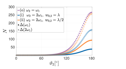
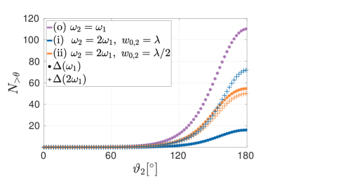
Figure 15: Partitioning of the attainable numbers of signal photons into the energy regimes $\Delta(\omega_{1})$ and $\Delta(2\omega_{1})$ for the various scenarios (o)-(ii). Both high-intensity laser pulses are polarized perpendicularly to the collision plane. The segment with center frequency ${\rm k}=\omega_{1}$ ($2\omega_{1}$) is depicted by $\bullet$ ($+$) symbols. Naturally, there is no ${\rm k}\approx 2\omega_{1}$ signal for the collision of two fundamental frequency beams. Top: Total number of signal photons $N$. Bottom: Integrated number of signal photons emitted outside the forward cones of the colliding Gaussian laser beams $N_{>\theta}$.

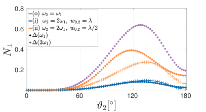
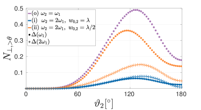
Figure 16: Partitioning of the perpendicularly polarized signal photons into the frequency regimes $\Delta(\omega_{1})$ and $\Delta(2\omega_{1})$ for the various scenarios (o)-(ii). Both high-intensity laser pulses are polarized perpendicularly to the collision plane. The segment with center frequency ${\rm k}=\omega_{1}$ ($2\omega_{1}$) is depicted by $\bullet$ ($+$) symbols. Naturally, no ${\rm k}\approx 2\omega_{1}$ signal is induced in the collision of two fundamental frequency beams. Top: Total number of perpendicularly polarized signal photons $N_{\perp}$. Bottom: Integrated number of perpendicularly polarized signal photons emitted outside the forward cones of the colliding Gaussian laser beams $N_{\perp,>\theta}$.

Analogously, Fig. 16 shows results for the number of signal photons polarized perpendicularly to the high-intensity laser beams $N_{\perp}$ and $N_{\perp,>\theta}$. Besides, in Tab. 2 we exemplarily stick to a collision angle of $\theta_{2}=135^{\circ}$ and provide explicit numerical values for the numbers of signal photons with energies in the ranges $\Delta(\omega_{1})$ and $\Delta(2\omega_{1})$. For a given energy regime $\Delta$, the values for $N$ and $N_{\perp}$ and analogously $n_{>\theta}=\frac{N_{>\theta}}{N}$ and $n_{\perp,>\theta}=\frac{N_{\perp,>\theta}}{N_{\perp}}$ exhibit similar trends.

Let us first detail on the behavior of $N$ and $N_{\perp}$. In the energy regime $\Delta(\omega)$, the largest numbers for $N$ and $N_{\perp}$ are obtained for scenario (o), followed by (ii) and finally (i). This is completely consistent with our expectations as the maximum number of frequency-$\omega_{1}$ signal photons is to be expected for the collision of two fundamental-frequency beams. As one can see in Fig. 7, these essentially elastically scattered signal photons are predominantly emitted in the forward directions of the high-intensity laser beams. The finding that the attainable signal photon numbers in scenario (ii) are larger than for scenario (i) hints at the fact that the peak field strength is most decisive for the effect. Recall, that for (ii) the frequency-doubled laser beam is focused down to the diffraction limit with $f^{\#}=1$, guaranteeing a maximum peak field, while in (i) it is only focused with $f^{\#}=2$; cf. Figs. 12 and 13. In the energy regime $\Delta(2\omega_{1})$, we find similar trends for the behavior of $N$ and $N_{\perp}$. Generically, no frequency-$2\omega$ signal is generated in the collision of (o) two fundamental-frequency laser beams; see Eq. (33).

Secondly, we comment on the trends observed for the relative fractions of signal photons $n_{>\theta}$ and $n_{\perp,>\theta}$ scattered outside the beam divergences in forward direction. Again we first discuss the results obtained for the energy regime $\Delta(\omega_{1})$. This signal is mainly induced in the propagation direction of the high-intensity laser with fundamental frequency, which implies that effectively only the divergence of the fundamental-frequency beam matters. While the values of $n_{>\theta}$ and $n_{\perp,>\theta}$ are similar for the cases (o) and (i), the result for case (ii) is significantly different. For the cases (o) and (i), the fundamental frequency beam collides with a beam of similar transverse focus profile of width $w_{0,1}=w_{0,2}=\lambda$. As the signal photons are predominantly induced in the focus, the similar values obtained for $n_{>\theta}$ and $n_{\perp,>\theta}$ are not surprising.

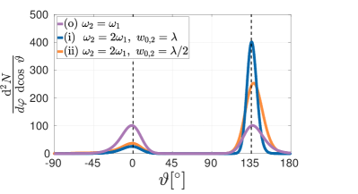
Figure 17: Differential number of signal photons $\frac{{\rm d}^{2}N}{{\rm d}\varphi\,{\rm d}\cos\vartheta}$ for $\varphi=0$, i.e., in the collision plane, for a collision angle of $\vartheta_{2}=135^{\circ}$, plotted as a function of the polar angle $\vartheta$ for the scenarios (o)-(ii). The dashed lines at $\vartheta=0^{\circ}$ ($\vartheta=135^{\circ}$) indicate the propagation direction of the high-intensity laser beam of frequency $\omega_{1}$ ($\omega_{2}$). The different peak-widths at $\vartheta\approx 135^{\circ}$ for scenarios (i) and (ii) can be traced back to the different focusing of the frequency-doubled laser. Generically, a harder focusing results in a wider far-field divergence.

Conversely, the smaller beam waist of the frequency-doubled beam in (ii) naturally gives rise to a larger fraction of photons scattered out of the divergence of the fundamental frequency beam as compared to (o) and (i). Generically, a tighter scattering center results in a wider angle distribution of the scattered light in the far-field; cf. Ref. Karbstein:2016lby for similar observations in a strong-field QED context.

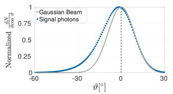
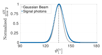
Figure 18: Comparison of the normalized differential number of signal photons $\frac{{\rm d}^{2}N}{{\rm d}\varphi\,{\rm d}\cos\vartheta}$ for $\varphi=0$ with the far-field photon distributions of the high-intensity laser beams. Here, we exemplarily limit ourselves to scenario (i) and a collision angle of $\vartheta_{2}=135^{\circ}$. As the frequency-doubled Gaussian beam is only focused to $w_{0,2}=\lambda$, its divergence fulfills $\theta_{2}=\theta_{1}/2$.

In the energy regime $\Delta(2\omega_{1})$, the ordering is reversed, such that the fraction of signal photons scattered out of the divergence of the high-intensity lasers is larger for (i) than for (ii). This observation can be explained along the same lines as above. The signal photons with energy in the regime $\Delta(2\omega_{1})$ are predominantly emitted in the vicinity of the propagation direction of the frequency-doubled laser beam, implying that the observed trends can be explained by considering the divergence of the $2\omega_{1}$ beam only. Now the frequency-doubled beam collides with a fundamental frequency pulse of the (i) same or (ii) wider width; cf. Figs. 12 and 13. Following the reasoning given above, this immediately implies that for (i) more signal photons are expected to be scattered outside the beam divergence of the high-intensity beam than for (ii).

In Fig. 17, we depict the differential number of signal photons $\frac{{\rm d}^{2}N}{{\rm d}\varphi\,{\rm d}\cos\vartheta}$ at $\varphi=0$ for all three scenarios (o)-(ii) For the symmetric configuration with two fundamental-frequency beams (o) both peaks are of the same height, and exhibit a mirror symmetry with respect to the middle axis between the two beams at $\vartheta=135^{\circ}/2=67.5^{\circ}$; see Fig. 7. In the scenarios (i) and (ii) the differential photon number are largest in the directions of the frequency-doubled beam.

For (o) and (ii) both high-intensity laser beams exhibit the same divergence $\theta_{1}=\theta_{2}$. Conversely, for (i) the divergence of the frequency-doubled beam is $\theta_{2}=\theta_{1}/2$, which explains why for (i) also the signal photons are scattered into a narrower far-field angle.

To allow for a comparison of the angular spread of the photons constituting the high-intensity laser beam and the signal photons, we plot the corresponding differential photon numbers in the far-field as a function of the polar angle $\vartheta$ in Fig. 18. The photon distributions of the high-intensity laser beams in the far-field scale as $\frac{{\rm d}^{2}N}{{\rm d}\varphi\,{\rm d}\cos\vartheta}\sim{\rm e}^{-2\vartheta^{2}/\theta_{1}^{2}}$ for the beam propagating along the $\rm z$ axis and as $\frac{{\rm d}^{2}N}{{\rm d}\varphi\,{\rm d}\cos\vartheta}\sim{\rm e}^{-2\left(\vartheta-\vartheta_{2}\right)^{2}/(\theta_{1}/f^{\#})^{2}}$ for the other beam; where $f^{\#}=1$ for both (o) and (ii), and $f^{\#}=2$ for (i). Obviously, the signal photons are scattered asymmetrically. The different decay of the signal photons and the photons constituting the high-intensity laser fields leads to an improved signal to background ratio.

VI Conclusions and Outlook

In this article, we have provided further evidence that all-optical signatures of quantum vacuum nonlinearity can be analyzed efficiently in terms of vacuum emission processes. The essence of this concept is that all macroscopically sourced fields are treated as classical, whereas the fields induced by quantum nonlinearities receive a quantum description in terms of signal photons. This concept matches ideally with the physical situation and thus provides direct access to physical observables.

In the present example of colliding laser pulses, this approach facilitates to directly determine the directional emission characteristics and polarization properties of the signal photons encoding the signature of quantum vacuum nonlinearities. Our main goal was to demonstrate that, assisted by a dedicated numerical algorithm, the vacuum emission approach is particularly suited to tackle signatures of strong-field QED in experimentally realistic electromagnetic field configurations generated by state-of-the-art high-intensity laser systems. To this end, we focused on a comparatively straightforward scenario, based upon the collision of two optical high-intensity laser pulses, which we model as pulsed Gaussian beams. Resorting to a locally constant field approximation of the Heisenberg-Euler effective action, our numerical algorithm allows for a numerically efficient and reliable study of the attainable numbers of signal photons for arbitrary collision angles and polarization alignments. Our formalism can be readily extended to the collision of more laser beams, such as the study of photon-merging Gies:2016czm , or equivalently four-wave mixing processes Lundstrom:2005za ; Lundin:2006wu induced by QED vacuum nonlinearities in the collision of three focused high-intensity laser beams.

Appendix A Convergence tests

As discussed in the main text, semi-analytical and numerical results fit almost perfectly for a suitable choice of numerical discretization parameters. In the following, we detail this choice of numerical parameters by studying the convergence of the numerical algorithm in comparison to the semi-analytical results for the toy-model benchmark test. Such an analysis is useful, because it (i) helps to improve the stability of the numerical results and (ii) yields systematic checks enabling to run simulations in regions of the parameter space, where no analytical reference values are available. Eventually, it also helps to minimize the program’s runtime as well as its memory requirements.

In this work, we have in total $10$ independent parameters controlling the numerical calculation. These are $N_{\rm x}$, $N_{\rm y}$, $N_{\rm z}$ specifying the lattice in the Cartesian grid for spatial/momentum coordinates, $N_{\varphi}$, $N_{\vartheta}$, $N_{\rm k}$ yielding the number of grid points in spherical momentum coordinates and $L_{\rm x}$, $L_{\rm y}$, $L_{\rm z}$, $L_{\rm k}$ defining the physical interval of length $2L_{\rm x,y,z,k}$ (sampling regions) of the corresponding variables centered around the region of interest. For illustration, we focus here on lower dimensional subsets. Similar convergence checks can be performed for each of these parameters.

In the following, we discuss the numerical convergence of our calculations in the context of two parameters, the radial momentum of the signal photons ${\rm k}$ and the longitudinal resolution of the pump fields along the ${\rm z}$ axis. For this, we first plot the total number of signal photons $N$ as a function of the number of grid points $N_{\Delta({\rm k})}$ for various choices of the momentum grid length $L_{\rm k}$ in Fig. 19. By comparison with the semi-analytical results we observe, that accuracy of the result increases with the momentum-space resolution as expected. It is also remarkable, that a few grid points in the total momentum ${\rm k}$, $\mathcal{O}(10)$, are sufficient in order to approximate the analytical solution reasonably well. The crucial ingredient is, of course, an appropriate choice for the resolved momentum interval: while the center of the $L_{\rm k}$ region can be adapted to the requirements imposed by energy conservation, cf. Eq. (33), being $k\simeq\omega$ in the present example, the size of $L_{\rm k}$ has to cover the bandwidth of the outgoing pulse. In the present case, a region with $L_{\rm k}\geq 0.3$eV is required, corresponding to $\geq 20\%$ of the central pulse energy. For instance, a region limited to $L_{\rm k}=0.1{\rm eV}$ is not sufficient to provide a precise estimate of the signal photon number, see Fig. 19.

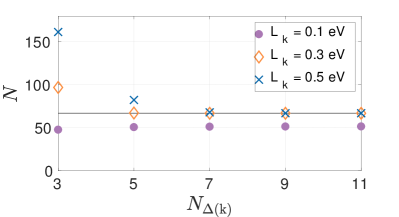
Figure 19: Convergence of the total number of signal photons $N$ as a function of the number of radial momentum grid points in $N_{\Delta({\rm k})}$ for various sizes of the sampling region. The sampling interval in ${\rm k}$ has a total length of $2L_{\rm k}$ and is centered around $\omega\approx 1.54{\rm eV}$. Two identical laser pulses ($\lambda=800{\rm nm}$, $W=25{\rm J}$, $\tau=25{\rm fs}$) are focused to $w_{0,1}=w_{0,2}=\lambda$. They are assumed to be polarized perpendicularly to the collision plane and collide under an angle of $\vartheta_{2}=135^{\circ}$. The benchmark toy model is used here to allow for a comparison with the semi-analytical result (black line).

Secondly, we investigate the spatial resolution needed in order to satisfactorily resolve the applied laser pulses. In this case, the parameters $L_{\rm z}$ and $N_{\rm z}$ have to meet two different requirements: on the one-hand side, $L_{\rm z}$ has to be chosen large enough to cover the region of interest given by the focal and collision region of the two pulses, while $N_{\rm z}$ has to be sufficiently large to precisely sample the details of the pulse shape; On the other hand, the nature of the Fourier transform implies that $\pi/(2L_{\rm z})$ defines an infrared cutoff and $\pi N_{\rm z}/(2L_{\rm z})$ an ultraviolet cutoff for the ${\rm z}$ component of the momentum of the outgoing signal photon. Hence, both have to be chosen sufficiently large also to resolve the sampling region $2L_{\rm k}$ centered around the peak momentum ${\rm k}$ of the signal photon appropriately. As a rule of thumb, an increase of the sampling region should go along with an increase of the number of grid points in order to keep the momentum space ultraviolet resolution (at least) constant.

In the present case, the procedure for choosing the discretization parameters is the following: The parameter $L_{\rm z}$ should be chosen large enough in order to resolve the focal region of the pump fields, i.e. at least one oscillation of the pump fields in the present case. Signal energy conservation suggests the signal photons to be located at around ${\rm k}\approx\omega$, the values for $L_{\rm z}$ and $N_{\rm z}$ should take on values such that the momentum region around $\omega$ is with sufficient resolution within the infrared and ultraviolet cutoffs induced by the Fourier transformation. For definiteness, we have fixed the longitudinal sampling region to ${\rm z}\in 2^{q}[-0.95\lambda,0.95\lambda]$ and study the convergence of the result for increasing $q$ and $N_{\rm z}$.

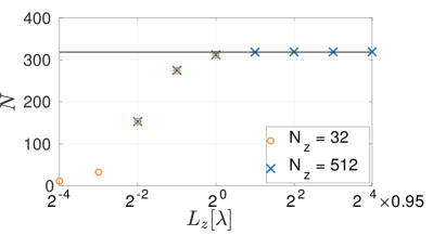
Figure 20: Convergence of the total number of signal photons $N$ as a function of the interval length $[-L_{\rm z},L_{\rm z}]$ for two sets of grid points in the ${\rm z}$ direction. Two identical laser pulses ($\lambda=800{\rm nm}$, $W=25{\rm J}$, $\tau=25{\rm fs}$) are focused to $w_{0,1}=w_{0,2}=\lambda$ and collide in a counter-propagation geometry. Both pulses are polarized perpendicularly to the collision plane. The benchmark toy model is used here to allow for a comparison with the semi-analytical result (black line).

The results for the signal photon number as a function of the size of the sampling region for two different grid resolutions are shown in Fig. 20 and Tab. 3. As expected, the spatial sampling region has to be large enough to cover the focal region of the size of a wavelength $\lambda$ in order to approach the correct result. We observe that even a rather small number of $32$ grid points can give an acceptable result with an error on the percent level, if the size of the sampling region is chosen appropriately as to cover the relevant momentum region of the signal photon upon Fourier transformation. For a reliable result with an error well below 1%, larger numbers of grid points and a sufficiently large sampling region are required – of course, at the expense of computing time.

Table 3: Benchmark calculations for the total number of signal photons attainable in the toy-model scenario. Two identical laser pulses ($\lambda=800{\rm nm}$, $W=25{\rm J}$, $\tau=25{\rm fs}$), focused to $w_{0,1}=w_{0,2}=\lambda$ and polarized perpendicularly to the collision plane, collide under an angle of $\vartheta_{2}=180^{\circ}$. The overall runtime and the corresponding mean relative error $\text{MRE}_{N}$ with respect to the semi-analytical result ($N=330.189$) are listed as functions of the grid size $L_{\rm z}$ and the number of grid points $N_{\rm z}$.

		Mean rel. error $\text{MRE}_{N}[\%]$
		Grid size $L_{\rm z}$ [$0.95\ {\rm\lambda}$]
$N_{\rm z}$	Runtime [s]	$2^{-1}$	$2^{0}$	$2^{1}$
32	1120	15.25	2.17	-
128	3105	14.87	2.20	0.22
512	9400	14.86	2.20	0.22

References

- (1) W. Heisenberg and H. Euler, Z. Phys. 98, 714 (1936), an English translation is available at [physics/0605038].
- (2) V. Weisskopf, Kong. Dans. Vid. Selsk., Mat.-fys. Medd. XIV, 6 (1936).
- (3) J. S. Schwinger, Phys. Rev. 82, 664 (1951).
- (4) W. Dittrich and M. Reuter, Lect. Notes Phys. 220, 1 (1985).
- (5) W. Dittrich and H. Gies, Springer Tracts Mod. Phys. 166, 1 (2000).
- (6) M. Marklund and J. Lundin, Eur. Phys. J. D 55, 319 (2009) [arXiv:0812.3087 [hep-th]].
- (7) G. V. Dunne, Eur. Phys. J. D 55, 327 (2009) [arXiv:0812.3163 [hep-th]].
- (8) T. Heinzl and A. Ilderton, Eur. Phys. J. D 55, 359 (2009) [arXiv:0811.1960 [hep-ph]].
- (9) A. Di Piazza, C. Muller, K. Z. Hatsagortsyan and C. H. Keitel, Rev. Mod. Phys. 84, 1177 (2012) [arXiv:1111.3886 [hep-ph]].
- (10) G. V. Dunne, Int. J. Mod. Phys. A 27, 1260004 (2012) [Int. J. Mod. Phys. Conf. Ser. 14, 42 (2012)] [arXiv:1202.1557 [hep-th]].
- (11) R. Battesti and C. Rizzo, Rept. Prog. Phys. 76, 016401 (2013) [arXiv:1211.1933 [physics.optics]].
- (12) B. King and T. Heinzl, High Power Laser Science and Engineering, 4, e5 (2016) [arXiv:1510.08456 [hep-ph]].
- (13) F. Karbstein, arXiv:1611.09883 [hep-th].
- (14) J. S. Toll, Ph.D. thesis, Princeton Univ., 1952 (unpublished).
- (15) R. Baier and P. Breitenlohner, Act. Phys. Austriaca 25, 212 (1967); Nuov. Cim. B 47 117 (1967).
- (16) H. Euler and B. Kockel, Naturwiss. 23, 246 (1935).
- (17) R. Karplus and M. Neuman, Phys. Rev. 80, 380 (1950); Phys. Rev. 83, 776 (1951).
- (18) R. N. Lee, A. I. Milstein and V. M. Strakhovenko, Phys. Rev. A 57, 2325 (1998) [hep-ph/9804386].
- (19) S. Z. Akhmadaliev, et al., Phys. Rev. C 58, 2844 (1998).
- (20) S. Z. Akhmadaliev, et al., Phys. Rev. Lett. 89, 061802 (2002) [hep-ex/0111084].
- (21) D. d’Enterria and G. G. da Silveira, Phys. Rev. Lett. 111, 080405 (2013) Erratum: [Phys. Rev. Lett. 116, 129901 (2016)] [arXiv:1305.7142 [hep-ph]].
- (22) M. Aaboud et al. [ATLAS Collaboration], Nature Phys. 13, 852 (2017) [arXiv:1702.01625 [hep-ex]].
- (23) R. P. Mignani, V. Testa, D. G. Caniulef, R. Taverna, R. Turolla, S. Zane and K. Wu, Mon. Not. Roy. Astron. Soc. 465, 492 (2017) [arXiv:1610.08323 [astro-ph.HE]].
- (24) L. M. Capparelli, L. Maiani and A. D. Polosa, Eur. Phys. J. C 77, 754 (2017) [arXiv:1705.01540 [astro-ph.HE]].
- (25) R. Turolla, S. Zane, R. Taverna, D. G. Caniulef, R. P. Mignani, V. Testa and K. Wu, arXiv:1706.02505 [astro-ph.HE].
- (26) G. Cantatore [PVLAS Collaboration], Lect. Notes Phys. 741, 157 (2008); E. Zavattini et al. [PVLAS Collaboration], Phys. Rev. D 77, 032006 (2008) [arXiv:0706.3419 [hep-ex]]; F. Della Valle et al., New J. Phys. 15 053026 (2013) [arXiv:1301.4918 [quant-ph]]; F. Della Valle et al., Eur. Phys. J. C 76, 24 (2016). [arXiv:1510.08052 [physics.optics]].
- (27) P. Berceau, R. Battesti, M. Fouché and C. Rizzo, Can. J. Phys. 89, 153 (2011); P. Berceau, M. Fouché, R. Battesti and C. Rizzo, Phys. Rev. A, 85, 013837 (2012) [arXiv:1109.4792 [physics.optics]]; A. Cadène, P. Berceau, M. Fouché, R. Battesti and C. Rizzo, Eur. Phys. J. D 68, 16 (2014) [arXiv:1302.5389 [physics.optics]].
- (28) X. Fan et al., Eur. Phys. J. D 71, 308 (2017) [arXiv:1705.00495 [physics.ins-det]].
- (29) G. Zavattini, F. Della Valle, A. Ejlli and G. Ruoso, arXiv:1601.03986 [physics.optics].
- (30) T. Inada, T. Yamazaki, T. Yamaji, Y. Seino, X. Fan, et al., Applied Sciences 7 (2017).
- (31) T. Heinzl, B. Liesfeld, K. -U. Amthor, H. Schwoerer, R. Sauerbrey and A. Wipf, Opt. Commun. 267, 318 (2006) [hep-ph/0601076].
- (32) A. Di Piazza, K. Z. Hatsagortsyan and C. H. Keitel, Phys. Rev. Lett. 97, 083603 (2006) [hep-ph/0602039].
- (33) V. Dinu, T. Heinzl, A. Ilderton, M. Marklund and G. Torgrimsson, Phys. Rev. D 89, 125003 (2014) [arXiv:1312.6419 [hep-ph]]; Phys. Rev. D 90, 045025 (2014) [arXiv:1405.7291 [hep-ph]].
- (34) F. Karbstein, H. Gies, M. Reuter and M. Zepf, Phys. Rev. D 92, 071301 (2015) [arXiv:1507.01084 [hep-ph]].
- (35) H. -P. Schlenvoigt, T. Heinzl, U. Schramm, T. Cowan and R. Sauerbrey, Physica Scripta 91, 023010 (2016).
- (36) F. Karbstein and C. Sundqvist, Phys. Rev. D 94, 013004 (2016) [arXiv:1605.09294 [hep-ph]].
- (37) B. King and N. Elkina, Phys. Rev. A 94, 062102 (2016) [arXiv:1603.06946 [hep-ph]].
- (38) S. Bragin, S. Meuren, C. H. Keitel and A. Di Piazza, arXiv:1704.05234 [hep-ph].
- (39) E. Lundstrom, G. Brodin, J. Lundin, M. Marklund, R. Bingham, J. Collier, J. T. Mendonca and P. Norreys, Phys. Rev. Lett. 96, 083602 (2006) [hep-ph/0510076].
- (40) J. Lundin, M. Marklund, E. Lundstrom, G. Brodin, J. Collier, R. Bingham, J. T. Mendonca and P. Norreys, Phys. Rev. A 74, 043821 (2006) [hep-ph/0606136].
- (41) B. King and C. H. Keitel, New J. Phys. 14, 103002 (2012) [arXiv:1202.3339 [hep-ph]].
- (42) H. Gies, F. Karbstein and N. Seegert, New J. Phys. 17, 043060 (2015) [arXiv:1412.0951 [hep-ph]].
- (43) H. Gies, F. Karbstein and N. Seegert, New J. Phys. 15, 083002 (2013) [arXiv:1305.2320 [hep-ph]].
- (44) V.P. Yakovlev, Zh. Eksp. Teor. Fiz. 51, 619 (1966) [Sov. Phys. JETP 24, 411 (1967)].
- (45) A. Di Piazza, K. Z. Hatsagortsyan and C. H. Keitel, Phys. Rev. Lett. 100, 010403 (2008) [arXiv:0708.0475 [hep-ph]]; Phys. Rev. A 78, 062109 (2008) [arXiv:0906.5576 [hep-ph]].
- (46) H. Gies, F. Karbstein and R. Shaisultanov, Phys. Rev. D 90, 033007 (2014) [arXiv:1406.2972 [hep-ph]].
- (47) H. Gies, F. Karbstein and N. Seegert, Phys. Rev. D 93, 085034 (2016) [arXiv:1603.00314 [hep-ph]].
- (48) S. L. Adler, J. N. Bahcall, C. G. Callan and M. N. Rosenbluth, Phys. Rev. Lett. 25, 1061 (1970).
- (49) Z. Bialynicka-Birula and I. Bialynicki-Birula, Phys. Rev. D 2, 2341 (1970).
- (50) S. L. Adler, Annals Phys. 67, 599 (1971).
- (51) V. O. Papanyan and V. I. Ritus, Zh. Eksp. Teor. Fiz. 61, 2231 (1971) [Sov. Phys. JETP 34, 1195 (1972)].
- (52) A. Di Piazza, A. I. Milstein and C. H. Keitel, Phys. Rev. A 76, 032103 (2007) [arXiv:0704.0695 [hep-ph]].
- (53) B. King, A. Di Piazza and C. H. Keitel, Nature Photon. 4, 92 (2010) [arXiv:1301.7038 [physics.optics]]; Phys. Rev. A 82, 032114 (2010) [arXiv:1301.7008 [physics.optics]].
- (54) D. Tommasini and H. Michinel, Phys. Rev. A 82, 011803 (2010) [arXiv:1003.5932 [hep-ph]].
- (55) K. Z. Hatsagortsyan and G. Y. Kryuchkyan, Phys. Rev. Lett. 107, 053604 (2011).
- (56) F. Karbstein and R. Shaisultanov, Phys. Rev. D 91, 113002 (2015) [arXiv:1412.6050 [hep-ph]].
- (57) B. King, P. Böhl and H. Ruhl, Phys. Rev. D 90, 065018 (2014) [arXiv:1406.4139 [hep-ph]].
- (58) P. Böhl, B. King and H. Ruhl, Phys. Rev. A 92, 032115 (2015) [arXiv:1503.05192 [physics.plasm-ph]].
- (59) A. Pons Domenech, H. Ruhl, arXiv:1607.00253 [physics.comp-ph]
- (60) P. Carneiro, T. Grismayer, R. Fonseca and L. Silva, arXiv:1607.04224 [physics.plasm-ph].
- (61) F. Karbstein, arXiv:1510.03178 [hep-ph].
- (62) H. Gies and F. Karbstein, JHEP 1703, 108 (2017) [arXiv:1612.07251 [hep-th]].
- (63) F. Karbstein and R. Shaisultanov, Phys. Rev. D 91, 085027 (2015) [arXiv:1503.00532 [hep-ph]].
- (64) G. V. Galtsov and N. S. Nikitina, Zh. Eksp. Teor. Fiz. 84, 1217 (1983) [Sov. Phys. JETP 57, 705 (1983)].
- (65) A. E. Siegman, Lasers, 1st. ed. (University Science Books, Herndon, VA, 1986); B. E. A. Saleh and M. C. Teich, Fundamentals of Photonics, 1st ed. (John Wiley & Sons, New York, USA, 1991).
- (66) F. Karbstein and E. A. Mosman, Phys. Rev. D 96, 116004 (2017) [arXiv:1711.06151 [hep-ph]].
- (67) W. Dittrich and H. Gies, Phys. Rev. D 58, 025004 (1998) [hep-ph/9804375].