A Theoretical Study of Aqueous Humor Secretion Based on a Continuum Model Coupling Electrochemical and Fluid-Dynamical Transmembrane Mechanisms

Abstract.

Intraocular pressure, resulting from the balance of aqueous humor (AH) production and drainage, is the only approved treatable risk factor in glaucoma. AH production is determined by the concurrent function of ionic pumps and aquaporins in the ciliary processes but their individual contribution is difficult to characterize experimentally. In this work, we propose a novel unified modeling and computational framework for the finite element simulation of the role of the main ionic pumps involved in AH secretion, namely, the sodium-potassium pump, the calcium-sodium pump, the anion channel and the hydrogenate-sodium pump. The theoretical model is developed at the cellular scale and is based on the coupling between electrochemical and fluid-dynamical transmembrane mechanisms characterized by a novel description of the electric pressure exerted by the ions on the intrachannel fluid that includes electrochemical and osmotic corrections. Considering a realistic geometry of the ionic pumps, the proposed model is demonstrated to correctly predict their functionality as a function of (1) the permanent electric charge density over the channel pump surface; (2) the osmotic gradient coefficient; (3) the stoichiometric ratio between the ionic pump currents enforced at the inlet and outlet sections of the channel. In particular, theoretical predictions of the transepithelial membrane potential for each simulated pump/channel allow us to perform a first significant model comparison with experimental data for monkeys. This is a significant step for future multidisciplinary studies on the action of molecules on AH production.

Keywords: ionic channels, eye, ionic pumps, aqueous humor, mathematical modeling, simulation, finite element method.

1. Introduction

The flow of aqueous humor (AH) and its regulation play an important role in ocular physiology by contributing to control the level of intraocular pressure (IOP) [35, 27]. Elevated IOP is the only approved treatable risk factor in glaucoma, an optic neuropathy characterized by a multifactorial aetiology with a progressive degeneration of retinal ganglion cells that ultimately leads to irreversible vision loss [17, 55]). Currently, glaucoma affects more than 60 million people worldwide and is estimated to reach almost 80 millions by 2020 [36]. IOP can be lowered via hypotonizing eye drops and/or surgical treatment,and it can be shown that reducing IOP by $1\;\mathrm{mmHg}$ has the effect of reducing the risk of glaucoma progression and subsequent vision loss by 10% [18].

Several classes of IOP-lowering medications are available for use in patients with glaucoma, including prostaglandin analogues, beta-blockers, carbonic anhydrase inhibitors, alpha-2-adrenergic agonists, in fixed and variable associations, while newer classes are still in clinical trials, such as the rho kinase inhibitors [16, 20, 37]. All currently available IOP-lowering agents function by altering AH production or drainage. However, differences in drug efficacy have been observed among patients that cannot be completely explained without a clear understanding of the mechanisms regulating AH flow. Motivated by this need, in this work we focus on AH production and we propose a mathematical approach to model and simulate the contribution of ionic pumps and channels to determine AH flow.

The production of AH takes places in the ciliary processes within the ciliary body, where clear liquid flows across the ciliary epithelium, a two-layered structure composed by an inner nonpigmented layer, representing the continuation of retinal pigmented epithelium, and an external nonpigmented layer, representing the continuation of the retina [15], as illustrated in Figure 1.

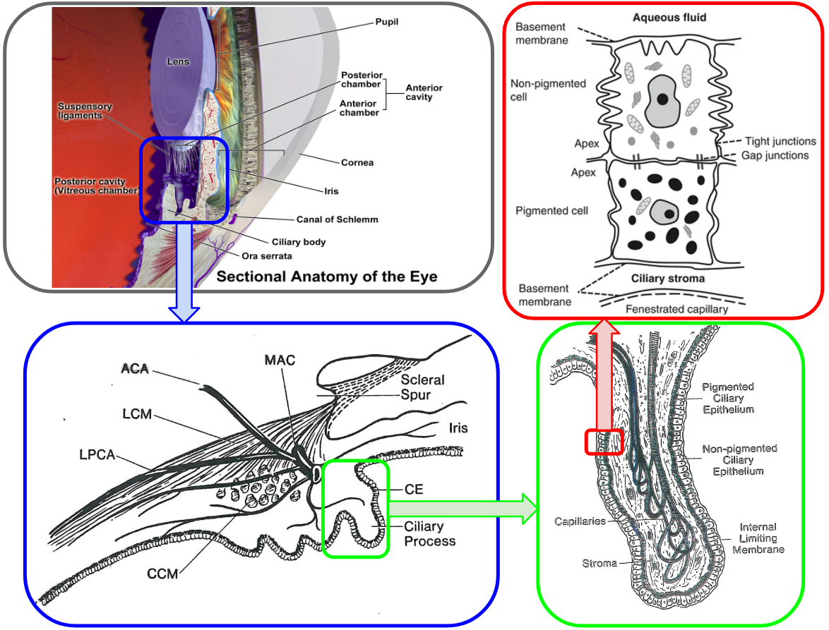
Figure 1.
Left top panel: anatomy of the eye and of the structures involved in aqueous humor production and regulation. (Blausen.com staff(2014). ”Medical gallery of Blausen Medical 2014”. WikiJournal of Medicine 1(2). DOI:10.15347/wjm/2014.010. ISSN 2002-4436)
Left bottom panel: MAC: major arterial circle; ACA: anterior ciliary arteries; LPCA: long posterior ciliary artery; LCM: longitudinal (fibers) ciliary muscle; CCM: circular (fibers) ciliary muscle; CE: ciliary epithelium (figure reproduced from [47])
Right bottom panel: A ciliary process is composed by capillaries, stroma and two layer of epithelium (inner, pigmented and outer, nonpigmented) (figure reproduced from [47])
Right top panel: the two-layer structure of the ciliary epithelium (figure reproduced from https://entokey.com/wp-content/uploads/2016/).

Three main mechanisms are involved in the production of AH: (i) convective delivery of fluid and metabolic components via the ciliary circulation; (ii) ultrafiltration and diffusion of fluid and metabolic components across the epithelial cells driven by gradients in hydrostatic pressure, oncotic pressure and metabolite concentrations; (iii) active secretion into the posterior chamber driven by increased ionic concentrations within the basolateral space between nonpigmented epithelial cells.

In this work we focus on the third mechanism, henceforth referred to as AH secretion, which is responsible for approximately $80-90\%$ of the whole AH production process [14, 31]. More precisely, we aim at modeling the selective movement of anions and cations across the membrane of the nonpigmented epithelial cells, the resulting gradient of ion and solute concentrations across the membrane, and the induced fluid egression into the posterior chamber.

The proposed simulation of AH secretion presents many challenges from the modeling viewpoint. Existing references concerning AH secretion are primarily based on lumped parameter models that provide a systemic view of AH flow [6, 28, 50], but do not reproduce the detailed phenomena occurring at the level of single ionic pumps. Detailed models based on the Velocity-Extended Poisson-Nerst-Planck (VE-PNP) system have been utilized to simulate electro-kinetic flows [25, 3, 4], but different models for the volumetric force coupling electrochemical and fluid-dynamical mechanisms have been proposed [49, 39, 40, 12], thereby raising the question of which one, if any, is the most appropriate for the application at hand. In addition, some of the most important parameters in the VE-PNP model, such as the concentration of ions within the ionic channel, the fixed charge on the channel lateral surface, the osmotic diffusive parameter, cannot be easily accessed experimentally and so are not readily available in the literature. In the pilot investigation conducted in [34], we explored the feasibility of utilizing a VE-PNP model to simulate the sodium-potassium pump (Na⁺-K⁺) within the nonpigmented epithelial cells of the eye. However, several other ionic pumps and channels are involved in AH secretion  [27], and have not yet been modeled in the context of AH flow.

The present work aims at extending the modeling and simulation treatment of [34] through the development of a unified framework capable of simulating AH secretion by including the four main ionic pumps and channels involved in the process, namely, the calcium-sodium pump (Ca⁺⁺-Na⁺), the carbonic anhydrase-activated anion channel (Cl^- - HCO${}_{3}^{-}$) and sodium-hydrogen exchanger (Na⁺-H⁺). The computational structure used in the numerical simulations is based on the adoption of (1) a temporal semi-discretization with the Backward Euler method; (2) a Picard iteration to successively solve the equation system at each discrete time level; and (3) a spatial discretization of each differential subproblem obtained from system decoupling using the Galerkin Finite Element Method. Numerical simulations are utilized to: (i) compare how and to what extent different modeling choices for the volumetric coupling force affect the resulting transmembrane potential, stoichiometric ratio and intrachannel fluid velocity; and (ii) characterize the correct boundary conditions and the value of the permanent electric charge density on the channel lateral surface that allow us to predict a biophysically reasonable behavior of ionic pumps and channels in realistic geometries. Overall, this work provides the first systematic investigation of VE-PNP models in the context of AH secretion and paves the way to future studies on biochemical, pharmacological and therapeutical aspects of AH flow regulation.

The paper is organized as follows. Section 2 provides a brief functional description of the main features pertaining the Na⁺-K⁺, Ca⁺⁺-Na⁺ and Cl^- - HCO${}_{3}^{-}$ pumps and the Na⁺-H⁺ channel. The VE-PNP system is described in Section 3 and the mathematical model for the volume force density in the right-hand side of the linear momentum balance equation for the intrachannel fluid is described in Section 4. The numerical discretization of the VE-PNP model equations is discussed in Section 5, whereas simulation results of the effect of volumetric forces and permanent electric charge density are presented in Sections 6 and 7, respectively. Model limitations, conclusions and future perspectives are outlined in Section 8.

2. Ionic pumps and channels in AH secretion

In this section we provide a short description of the main ionic pumps and channels that are involved in the process of AH secretion. We refer to [19] for an overview of ionic channels in cellular biology and to [26] for a mathematical analysis of ionic pumps in cellular biology.

Figure 2. Schematic diagram of ionic pumps and ionic channels located on the lipid membrane in the nonpigmented epithelial cells of the ciliary body of the eye. Aqueous humor is produced by the active secretion of fluid through the ionic channels during their activity. This figure is inspired by Figure 9 of [46].

2.1. The sodium-potassion ATPasi pump.

This pump plays a fundamental role in cellular biology as it is present in the membrane of every cell in the human body. The enzyme ATPasi, located either in pigmented or nonpigmented ciliary epithelium, causes the hydrolysis of one molecule of ATP and produces the necessary energy to expel three Na⁺ ions, while allowing two K⁺ ions to enter. This process is not electrically neutral as it entails an outflux of three positive charged particles of sodium and an influx of only two positive charged particles of potassium. The ion outflux and influx are schematically represented in Figure 3.

Figure 3. Schematic representation of the Na⁺-K⁺ pump. The stoichiometric ratio is $3:2$, since there is an outflux of three Na⁺ ions and an influx of two K⁺ ions.

2.2. The calcium-sodium ATPasi pump.

This pump is activated when calcium accumulates inside the cell above a certain threshold, that is usually around $1\;\mathrm{mM}$. This pump entails the influx of three Na⁺ ions and an outflux of one Ca⁺⁺ ion. As in the previous case, this process is not electrically neutral as three positive sodium ions enter the cell whereas only one positive calcium ion exits the cell. The ion outflux and influx are schematically represented in Figure 4.

Figure 4. Schematic representation of the Ca⁺⁺-Na⁺ pump. The stoichiometric ratio is $3:1$, since there is an influx of three Na⁺ ions and an outflux of one Ca⁺⁺ ion.

2.3. The carbonic anhydrase-activated anionic pump.

This pump involves the movement of negative ions. Carbonic anhydrase is an enzyme that mediates the transport of bicarbonate across the ciliary epithelium to maintain the homeostatic balance of carbonate across the cell membrane. More precisely, carbonic anhydrase favors the splitting of one molecule of H₂CO₃ into a positive H⁺ ion and a negative HCO${}_{3}^{-}$ ion. Then, the HCO${}_{3}^{-}$ ion exits the cell through the anion channel with an exchange of a chlorine ion Cl^- that enters the cell. The balance of this pump is electrically neutral because for every negative charged HCO${}_{3}^{-}$ leaving the cell there is a negative charged Cl^- ion entering the cell [54]. The ion outflux and influx are schematically represented in the top panel of Figure 5.

Figure 5. Schematic representation of the carbonic anhydrase-activated anionic pump (top panel) and of the Na⁺ and H⁺ exchanger (bottom panel). The stoichiometric ratio of the anionic pump is $1:1$, since there is an influx of one Cl^- ion and an outflux of one HCO${}_{3}^{-}$ ion. The stoichiometric ratio of the Na⁺ and H⁺ exchanger is also 1:1, since there is an influx of one Na⁺ ion and an outflux of one H⁺ ion.

2.4. Na⁺ and H⁺ exchanger.

This pump is strictly correlated with the activity of the carbonic anhydrase-activated anionic pump previously described. A positive H⁺ ion resulting from the splitting reaction of one molecule of H₂CO₃ exits the cell with an exchange of one Na⁺ ion entering the cell. Thus, this pump is electrically neutral. The ion outflux and influx are schematically represented in the bottom panel of Figure 5.

3. The mathematical model

In this section we illustrate the system of partial differential equations (PDEs) constituting the mathematical model at the cellular scale level of ionic channel and pumps that activate the AH secretion. We refer to [43] for a detailed discussion of the analytical properties of the model equations and of the numerical methods used for their discretization, and to [34] for preliminary results on the adoption of the model in the study of the role of bicarbonate ion to correctly determine the electrostatic potential drop across the cellular membrane at the level of eye transepitelium.

Figure 6. Cross-section of a simplified ionic channel geometry. The lipid membrane bilayer is represented in brown color. The ion channel is represented in cyan color. The portions of the boundary $\partial\Omega$ are labeled as $sideA$ (intracellular side), $sideB$ (extracellular side) and $\Gamma_{LAT}$ (lateral surface).

The geometrical setting that we consider henceforth is the computational domain $\Omega$ illustrated in Figure 6 representing a cross-section of a simplified ion channel geometry. Such representation includes any of the ionic pumps or ionic channels described in Section 2, which are located on the lipid bilayer constituting the membrane of the nonpigmented epithelial cells of the ciliary body of the eye schematically depicted in Figure 1 (right top panel). We indicate by $\partial\Omega$ the boundary of $\Omega$, by $\underline{n}$ the outward unit normal vector on $\partial\Omega$ and by $sideA$, $sideB$ and $\Gamma_{LAT}$ the intracellular surface, the extracellular surface and the lateral boundary, respectively, in such a way that $\partial\Omega=sideA\cup sideB\cup\Gamma_{LAT}$. For a given starting time $t_{0}$ and a given observational time window $T_{obs}$, we set $I_{T}:=(t_{0},t_{0}+T_{obs})$ and we denote by $Q_{T}:=\Omega\times I_{T}$ the space-time cylinder in which we study the spatial and temporal evolution of the process of AH secretion at the cellular scale level. To clarify the physical foundation of the cellular scale model object of the present article, we assume that the following strongly coupled mechanisms concur to determine AH secretion:

• electric field formation: this mechanism is determined by the mutual interaction among ions in the intrachannel fluid and their interaction with the permanent electric charge density distributed on the surface of the channel structure. Mathematically, the mechanism is described by the Poisson equation, supplied by appropriate boundary conditions at the inlet and outlet sections of the channel and on its external surface;

• ion motion: this mechanism is determined by the superposition of a diffusion process driven by ion concentration gradients along the channel and of a drift process driven by the force exerted by the electric field on each ion charged particle. Mathematically, the mechanism is described by the Nernst-Planck equations, supplied by appropriate initial conditions inside the channel and by appropriate boundary conditions at the inlet and outlet sections of the channel and on its external surface;

• fluid motion: this mechanism is determined by the volume force density that is exerted by the charged ion particles because of their motion inside the channel. Mathematically, the mechanism is described by the time-dependent Stokes equations, supplied by appropriate initial conditions inside the channel and by appropriate boundary conditions at the inlet and outlet sections of the channel and on its external surface.

We refer to the resulting mathematical model as Velocity-Extended Poisson-Nernst-Planck system (VE-PNP) [42, 23, 45, 24]. The VE-PNP system can be derived by the application of the following physical laws [43]: (i) mass balance for each of the $M$ chemical species included in the system (1a); (ii) linear momentum balance for each chemical species (1b); (iii) electrical charge conservation (1c); (iv) mass balance for intrachannel fluid (1f); (v) linear momentum balance for intrachannel fluid (1g). Ultimately, the system consists of the following set of PDEs to be solved in $Q_{T}$:

(1a) $$\frac{\partial n_{i}}{\partial t}+\text{div}\,\underline{f}_{i}=0 \forall i=1,\dots,M$$

(1b) $$\underline{f}_{i}=\frac{z_{i}}{|z_{i}|}\mu_{i}n_{i}\underline{E}-D_{i}\nabla n_{i}+\boxed{n_{i}\,\underline{u}} \forall i=1,\dots,M$$

(1c) $$\text{div}\underline{D}=q\sum_{i=1}^{M}z_{i}n_{i}+q\rho_{fixed}$$

(1d) $$\underline{D}=\epsilon_{f}\underline{E}$$

(1e) $$\underline{E}=-\nabla\varphi$$

(1f) $$\text{div}\,\underline{u}=0$$

(1g) $$\rho_{f}\frac{\partial\underline{u}}{\partial t}=\text{div }\underline{\underline{\sigma}}(\underline{u},p)+\boxed{\underline{F}_{ion}}$$

(1h) $$\underline{\underline{\sigma}}(\underline{u},p)=2\mu_{f}\underline{\underline{\epsilon}}(\underline{u})-p\,\underline{\underline{\delta}}$$

(1i) $$\underline{\underline{\epsilon}}(\underline{u})=\underline{\underline{\nabla}}_{s}\underline{u}=\dfrac{1}{2}(\nabla\underline{u}+(\nabla\underline{u})^{T}).$$

The equation set (1) comprises two main blocks. Equations (1a)- (1e) constitute the Poisson-Nernst-Planck (PNP) block whereas equations (1f)- (1i) constitute the Stokes block. As far as the PNP block is concerned, $M$ is the number of ionic species, $\underline{f}_{i}$ denotes the ion particle flux $[\mathrm{cm^{-2}\,s^{-1}}]$, $n_{i}$ is the ion concentration $[\mathrm{cm^{-3}}]$, $\mu_{i}$ and $D_{i}$ are the ion electrical mobility $[\mathrm{cm^{2}\,V\,s^{-1}}]$ and diffusivity $[\mathrm{cm^{2}\,s^{-1}}]$ and $T$ is the absolute temperature $[\mathrm{K}]$. The mobility $\mu_{i}$ is proportional to the diffusivity $D_{i}$ through the Einstein relation

(2) $$D_{i}=\dfrac{K_{B}T}{q|z_{i}|}\mu_{i}\qquad i=1,\ldots,M,$$

where $q$ is the electron charge $[\mathrm{C}]$ and $K_{B}$ is the Boltzmann constant $[\mathrm{cm^{2}gs^{-2}K^{-1}}]$. In Eq. (1c) and Eq. (1e), $\underline{D}$ is the electric displacement $[\mathrm{C\,cm^{-2}}]$, $\underline{E}$ is the electric field $[\mathrm{V\,cm^{-1}}]$, $\varphi$ is the electric potential $[\mathrm{V}]$ and $\epsilon_{f}$ is the electrolyte fluid dielectric permittivity $[\mathrm{F\,cm^{-1}}]$. The quantity $z_{i}$ is the valence of the $i$-th ion ($z_{i}>0$ for cations, $z_{i}<0$ for anions) whereas $\rho_{fixed}$ is the permanent electric charge density $[\mathrm{C\,cm^{-3}}]$. We define the ionic current density $\underline{J}_{i}$ $[\mathrm{A\,cm^{-2}}]$ of each ion species as

(3) $$\underline{J}_{i}=qz_{i}\,\underline{f}_{i}\qquad i=1,\ldots,M.$$

As far as the Stokes block is concerned, $\underline{u}$ is the fluid velocity $[\mathrm{cm\,s^{-1}}]$ and fluid incompressibility is expressed by Eq. (1f). Eq. (1h) and Eq. (1i) are the constitutive laws for the stress tensor $[\mathrm{dyne\;cm^{-2}}]$ and the strain rate $[\mathrm{s^{-1}}]$ respectively, where $p$ denotes the fluid pressure $[\mathrm{dyne\;cm^{-2}}]$, $\mu_{f}$ is the fluid viscosity $[\mathrm{g\,cm^{-1}\,s^{-1}}]$, $\rho_{f}$ is the fluid mass density $[\mathrm{g\,cm^{-3}}]$ and $\underline{\underline{\delta}}$ the second-order identity tensor of dimension 3. Since the focus of the article is the investigation of the role of electrochemical forces on the secretion of AH across the nonpigmented epithelial cells in the ciliary body of the eye, we assume that the temperature $T$ of the intrachannel fluid is constant and equal to the value $T_{0}=293.75\mathrm{K}$. The boxed terms in Eq. (1b) and Eq. (1g) are the contributions that introduce the coupling between the PNP block of system (1) and the Stokes block of system (1). In particular,

(4) $$\underline{F}_{ion}=\sum_{i=1}^{M}\underline{F}_{i}$$

expresses the volume force density $[\mathrm{dyne\;cm^{-3}}]$ exerted by the ionic charges on the intrachannel fluid, the quantities $\underline{F}_{i}$ representing the contribution to the volume force density given by each ion species, $i=1,\ldots,M$.

The equation system (1) is equipped with the following initial conditions:

(5a) $$n_{i}(\underline{x},0)=n_{i}^{0}(\underline{x})\qquad i=1,\ldots,M,\qquad\underline{x}\in\Omega,$$

(5b) $$\underline{u}(\underline{x},0)=\underline{u}^{0}(\underline{x})\qquad\underline{x}\in\Omega,$$

where $$n_{i}^{0} \underline{u}^{0} \varphi^{0}=\varphi^{0}(\underline{x}) \underline{x}\in\Omega \partial\Omega n_{i}=n_{i}^{0} i=1,\ldots,M$$ are given positive functions and is a given function. The initial condition , , is the solution of the equation set (1c)- (1e), under appropriate boundary conditions on , having set , .

The boundary conditions associated with system (1) that are considered in the present article are of mixed Dirichlet-Neumann type. Their characterization for each equation in the system is specified in each simulation illustrated in Sections 6 and 7.

4. Model for the volume force density

In this section we discuss a general approach to the modeling of the volume force density $\underline{F}_{i}$ on the right-hand side in the linear momentum balance equation (1g). $\underline{F}_{i}$ expresses the contribution from the $i$-th ionic species, $i=1,\ldots,M$, to the total volume force density exerted by the ion charged particles on the intrachannel fluid and is assumed henceforth to be characterized by the following relation

(6) $$\underline{F}_{i}=qz_{i}n_{i}\;\underline{E}_{i}^{echs}-k_{osm}\,\nabla n_{i}\qquad i=1,\ldots,M.$$

The first term at the right-hand side of (6) represents the volume force density due to a generalized electrochemical field $\underline{E}_{i}^{echs}$ whereas the second term represents the volume force density due to an osmotic concentration gradient according to the parameter $k_{osm}$ $[\mathrm{N\;m}]$ (see [22]). The generalized electrochemical field is the result of the superposed effect of passive drift due to the electric field (e), the diffusion mechanism associated with a chemical concentration gradient (c) and the particle size exclusion effect associated with the hard sphere (hs) theory (see [41, 38]). Relation (6) is referred to henceforth as electrochemical model including osmotic and size exclusion mechanisms (echsk).

Assuming that $\underline{E}_{i}^{echs}$ is a gradient field, we have:

(7a) $$\underline{E}_{i}^{echs}=-\nabla\varphi_{i}^{echs}\qquad i=1,\ldots,M,$$

(7b) $$\varphi^{echs}_{i}=\varphi^{ec}_{i}+\mu_{i}^{ex}\qquad i=1,\ldots,M,$$

where $$\varphi^{ec}_{i} i$$ is the generalized electrochemical potential of the -th species

(7c) $$\varphi_{i}^{ec}=\varphi+\dfrac{V_{th}}{z_{i}}\ln\left(\dfrac{n_{i}}{n_{ref}}\right)\qquad i=1,\ldots,M$$

and $$\mu^{ex}_{i} i$$ is the exclusion effect potential of the -th species (see [5])

$$\mu_{i}^{ex}=-V_{th}\Big{[}\ln(1-\frac{4\pi}{3}\sum_{k=1}^{M}n_{k}R_{k}^{3})$$

$$+4\pi\frac{R_{i}(\sum_{k=1}^{M}n_{k}R_{k}^{2})+R_{i}^{2}(\sum_{k=1}^{M}n_{k}R_{k})+\dfrac{1}{3}R_{i}^{3}(\sum_{k=1}^{M}n_{k})}{1-\frac{4\pi}{3}\sum_{k=1}^{M}n_{k}R_{k}^{3}}$$

$$+\dfrac{16\pi^{2}}{3}\frac{R_{i}^{3}(\sum_{k=1}^{M}n_{k}R_{k})(\sum_{k=1}^{M}n_{k}R_{k}^{2})+\dfrac{3}{2}R_{i}^{2}\left(\sum_{k=1}^{M}n_{k}R_{k}^{2}\right)^{2}}{\left(1-\frac{4\pi}{3}\sum_{k=1}^{M}n_{k}R_{k}^{3}\right)^{2}}$$

(7d) $$+\dfrac{64\pi^{3}}{9}\frac{R_{i}^{3}\left(\sum_{k=1}^{M}n_{k}R_{k}^{2}\right)^{3}}{\left(1-\frac{4\pi}{3}\sum_{k=1}^{M}n_{k}R_{k}^{3}\right)^{3}}\Big{]}\qquad i=1,\ldots,M,$$

$$n_{ref} R_{i} [\mathrm{cm^{-3}}] i$$ and being a positive constant representing the reference concentration in the ionic solution and the ionic radius of the -th ion species, respectively.

Relation (6) is indeed a general view of the volume force density from which simpler expressions of $\underline{F}_{i}$ can be derived. These models constitute a hierarchy characterized by an increasing number of approximations and a consequent decreasing level of physical complexity.

echs:

Electrochemical model including hard sphere theory. This model is derived from (6) by neglecting the contribution of the osmotic gradient. This includes: the Coulomb electrical force associated with a charge density, the chemical gradient and size exclusion mechanisms. It is mathematically expressed by the following relation

(8) $$\underline{F}_{i}=qz_{i}n_{i}\;\underline{E}_{i}^{echs}\qquad i=1,\ldots,M.$$

ec:

Electrochemical model. This is derived from (8) neglecting the size exclusion phenomena. This includes the Coulomb electrical force associated with a charge density and the chemical gradient mechanism. It is mathematically expressed by the following relations:

(9) $$\underline{F}_{i}=qz_{i}n_{i}\;\underline{E}_{i}^{ec}\qquad i=1,\ldots,M.$$

(10) $$\underline{E}_{i}^{ec}=-\nabla\varphi_{i}^{ec}\qquad i=1,\ldots,M.$$

Stratton:

Stratton model. This model is derived from (9) by neglecting the contribution induced by the chemical gradient. This was originally proposed in [49] and it is widely adopted in the modeling description of electrokinetic phenomena (see [25]). It is mathematically expressed by the following relation

(11) $$\underline{F}_{i}=qz_{i}n_{i}\;\underline{E}\qquad i=1,\ldots,M.$$

eck:

Electrochemical model including osmotic force. This model is derived from (6) by neglecting the contribution of the size exclusion phenomena. This model includes the Coulomb electrical force associated with a charge density, the chemical and osmotic gradient mechanisms It is mathematically expressed by the following relation

(12) $$\underline{F}_{i}=qz_{i}n_{i}\;\underline{E}_{i}^{ec}-k_{osm}\,\nabla n_{i}\qquad i=1,\ldots,M.$$

The effect on intrachannel fluid modtion induced by the above force models is analyzed, in the context of the Na⁺-K^- pump, in Section 6 where the predicted electrolyte fluid velocity is compared with the volumetric force density $\underline{F}_{i}$ exerted by the ions on it.

5. Time advancing, functional iteration and numerical discretization

In this section we provide a short description of the algorithm that is used to numerically solve system (1). We refer to [43] for more details on the stability and convergence analysis of the adopted methods as well as their implementation in the general-purpose C++ modular numerical code MP-FEMOS (Multi-Physics Finite Element Modeling Oriented Simulator) that has been developed by some of the authors [33, 32, 1].

The VE-PNP model constitutes a nonlinearly coupled system of PDEs of incomplete parabolic type because of the fact that at each time level the electrostatic potential $\varphi$ and the electric field $\underline{E}$ must be updated as a function of the ion concentrations and of the fixed permanent charge by solving the elliptic Poisson equation (1c). In turn, the electric field $\underline{E}$ contributes to determine ion motion through the Nernst-Planck relation (1b) and fluid motion through the relation (6) for the volume force density.

To disentangle the various coupling levels that are present in the VE-PNP system, we proceed as follows:

1. we perform a temporal semi-discretization of the problem by resorting to the Backward Euler (BE) method;

2. we introduce a Picard iteration to successively solve the equation system at each discrete time level;

3. we perform a spatial discretization of each differential subproblem obtained from system decoupling using the Galerkin Finite Element Method (GFEM).

The use of the BE method has the twofold advantage that (a) it is unconditionally absolute stable and (b) it is monotone. Property (a) allows to take relatively large time steps thus reducing the computational effort to reach steady-state conditions. Property (b), combined with an analogous one for the spatial discretization scheme of the Nernst-Planck equations, ensures that the computed ion concentrations are positive for all discrete time levels.

The use of a Picard iteration has the twofold advantage that (c) it is a decoupled algorithm and (d) a maximum principle is satisfied by the solutions of two of the boundary value problems (BVP) obtained from decoupling. Property (c) amounts to transforming the nonlinearly coupled system (1) into the successive solution of three sets of linear BVPs of reduced size. Property (d) implies the existence of an invariant region for the electric potential depending only on the boundary data and on the fixed permanent charge and the positivity of the computed ion concentrations.

The use of the GFEM has the twofold advantage that (e) it can easily handle complex geometries and (f) provides an accurate and stable numerical approximation of the solution of each BVP obtained from system decoupling. Property (e) is implemented through the partition of the domain of biophysical interest into the union of tetrahedral elements of variable size. Property (f) is implemented through the use of piecewise linear finite elements for the Poisson equation, piecewise linear finite elements with exponential fitting stabilization along of mesh edges for the Nernst-Planck equations, and of the inf-sup stable Taylor-Hood finite element pair for the Stokes equations.

Figure 7 illustrates the flow-chart of the temporal semi-discretization for time advancing with the BE method and the Picard iteration used to successively solve the three linear equation subsystems.

Figure 7. Flow-chart of the computational algorithm to solve the VE-PNP system. The nonnegative integer $k$ is the temporal discretization counter. The nonnegative integer $j$ is the Picard iteration counter.

6. Comparison of volumetric force models on an idealized sodium-potassium pump

The aim of this section is to compare the different descriptions introduced in Section 4 of the volume force density $\underline{F}_{ion}$ exerted on the intrachannel fluid in the linear momentum balance equation (1g). In particular we investigate the biophysical reliability of the various models to describe the functionality of an idealized version of the Na⁺-K⁺ pump illustrated in Section 2 in which the simultaneous presence of Na⁺, K⁺, Cl^- and HCO${}_{3}^{-}$ ionic species is considered. The analysis criteria are based on the comparison of simulation results with (i) the electrostatic potential drop measured across the transepithelial membrane, (ii) the theoretical stoichiometric ratio $3:2$ and (iii) the direction of the AH flow from the cell into the basolateral space. The ideality of the Na⁺-K⁺ pump is represented by the geometry adopted for numerical simulation, consisting of the cylinder with axial length $L_{ch}=5\mathrm{nm}$ and radius $R_{ch}=0.4\mathrm{nm}$ shown in Figure 8 together with its partition into 37075 tetrahedral finite elements. We point out that the above geometrical setting, despite being a simplified approximation of the real structure, has been successfully employed for biological investigations in [1], [43] and [34].

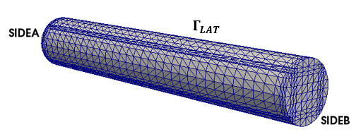
Figure 8. Computational domain for the simulation of the Na⁺-K⁺ pump. The finite element triangulation consists of 37075 tetrahedra.

6.1. Boundary and initial conditions

Because of the complexity of the boundary conditions (BCs) and initial conditions (ICs) involved in the simulation of the pump, it is useful to accurately describe them for each equation in (1).

6.1.1. Poisson equation

For all $t\in I_{T}$, the BCs for the Poisson equation (1c)-(1e) are:

(13a) $$\varphi=0 \qquad\textrm{on }sideA$$

(13b) $$\underline{D}\cdot\underline{n}=0 \qquad\textrm{on }sideB\cup \Gamma_{LAT}.$$

Condition (13a) has the scope of introducing a reference value for the calculation of the electrostatic potential drop across the cellular membrane. Condition (13b) expresses the biological fact that the aferomentioned potential drop is caused solely by the ion charge distribution within the channel because no external bias is applied.

6.1.2. Nernst-Planck equations

The Nernst-Planck equation system allows us to determine the spatial concentration of the various ion species inside the channel. The connection between the channel region and the intra/extracellular sides is made possible by enforcing nonhomogeneous Neumann boundary conditions that preserve the correct input/output biophysical pump functionality. The boundary and initial conditions for each simulated ion species read as follows:

K⁺:

(14a) $$\underline{f}_{\textrm{K}^{+}}\cdot\underline{n}=g_{\textrm{K}^{+}} \qquad\textrm{on }sideA$$

(14b) $$n_{\textrm{K}^{+}}=\textrm{K}^{+}_{out} \qquad\textrm{on }sideB$$

(14c) $$\underline{f}_{\textrm{K}^{+}}\cdot\underline{n}=0 \qquad\textrm{on }\Gamma_{LAT}$$

(14d) $$n_{\textrm{K}^{+}}(\underline{x},0)=\textrm{K}^{+}_{0} \qquad\forall\underline{x}\in\Omega.$$

Na⁺:

(14e) $$n_{\textrm{Na}^{+}}=\textrm{Na}^{+}_{in} \qquad\textrm{on }sideA$$

(14f) $$\underline{f}_{\textrm{Na}^{+}}\cdot\underline{n}=g_{\textrm{Na}^{+}} \qquad\textrm{on }sideB$$

(14g) $$\underline{f}_{\textrm{Na}^{+}}\cdot\underline{n}=0 \qquad\textrm{on }\Gamma_{LAT}$$

(14h) $$n_{\textrm{Na}^{+}}(\underline{x},0)=\textrm{Na}^{+}_{0} \qquad\forall\underline{x}\in\Omega.$$

Cl^-:

(14i) $$n_{\textrm{Cl}^{-}}=\textrm{Cl}^{-}_{in} \qquad\textrm{on }sideA$$

(14j) $$n_{\textrm{Cl}^{-}}=\textrm{Cl}^{-}_{out} \qquad\textrm{on }sideB$$

(14k) $$\underline{f}_{\textrm{Cl}^{-}}\cdot\underline{n}=0 \qquad\textrm{on }\Gamma_{LAT}$$

(14l) $$n_{\textrm{Cl}^{-}}(\underline{x},0)=\textrm{Cl}^{-}_{0} \qquad\forall\underline{x}\in\Omega.$$

HCO${}_{3}^{-}$:

(14m) $$n_{\textrm{HCO}^{-}_{3}}=\textrm{HCO}^{-}_{3,in} \qquad\textrm{on }sideA$$

(14n) $$n_{\textrm{HCO}^{-}_{3}}=\textrm{HCO}^{-}_{3,out} \qquad\textrm{on }sideB$$

(14o) $$\underline{f}_{\textrm{HCO}^{-}_{3}}\cdot\underline{n}=0 \qquad\textrm{on }\Gamma_{LAT}$$

(14p) $$n_{\textrm{HCO}^{-}_{3}}(\underline{x},0)=\textrm{HCO}^{-}_{3,0} \qquad\forall\underline{x}\in\Omega.$$

The values of the boundary data for the cations are specified in Table 12 whereas the values of the boundary data for the anions are specified in Table 13. The boundary values for the ions agree with the experimental value of the ionic concentrations measured in the intracellular and extracellular sides of the non-pigmented epithelial cells.

6.1.3. Stokes system

The calculation of fluid velocity is made possible by solving the Stokes system (1f)- (1g). To prescribe a correct biophysical condition of the intrachannel fluid we need to mathematically express that (1) the fluid is adherent to the channel wall; (2) no external pressure drop is applied across the channel; (3) the fluid is at the rest when the pump is not active. To this purpose, the appropriate BCs and ICs read:

(15a) $$\underline{u}=\underline{0} \qquad\textrm{on }\Gamma_{LAT}$$

(15b) $$\underline{\underline{{\sigma}}}\>\underline{n}=\underline{0} \qquad\textrm{on }sideA\cup sideB$$

(15c) $$\underline{u}(\underline{x},0)=\underline{0} \qquad\forall\underline{x}\in\Omega.$$

6.2. Simulation results

To ease the interpretation of the reported results, we point out that the $Z$ axis coincides with the axial direction of the channel and it is positively oriented towards the extracellular region. Reported data for the vector-valued variables (such as electric field, current densities and velocity) are the $Z$ component of the vectors because the other two computed components were comparably negligible. We set $\rho_{fixed}=0\;[\mathrm{C\,m^{-3}}]$, $t_{0}=0\;[\mathrm{s}]$ and $T_{obs}=50\;[\mathrm{ns}]$, a sufficiently large value to ensure that the simulated system has reached steady-state conditions at $t=T_{obs}$. The values of the dielectric permittivity of the intrachannel water fluid $\epsilon_{r}^{f}$, of the fluid shear viscosity $\mu_{f}$, of the fluid mass density $\rho_{f}$ and of the diffusion coefficients $D_{i}$ of each $i$-th ionic species involved in the computational tests are reported in Table 1. All the figures in the remainder of the section illustrate computed results at $t=T_{obs}$.

Model parameter	value	units
$\epsilon_{f}$	$708.32\cdot 10^{-10}$	$[\mathrm{Fcm^{-1}}]$
$\mu_{f}$	$10^{-2}$	$[\mathrm{gcm^{-1}s^{-1}}]$
$\rho_{f}$	$1$	$[\mathrm{gcm^{-3}}]$
$D_{\textrm{K}^{+}}$	$1.957\cdot 10^{-5}$	$[\mathrm{cm^{2}s^{-1}}]$
$D_{\textrm{Na}^{+}}$	$1.334\cdot 10^{-5}$	$[\mathrm{cm^{2}s^{-1}}]$
$D_{\textrm{Cl}^{-}}$	$2.033\cdot 10^{-5}$	$[\mathrm{cm^{2}s^{-1}}]$
$D_{\textrm{HCO}_{3}^{-}}$	$1.185\cdot 10^{-5}$	$[\mathrm{cm^{2}s^{-1}}]$
$D_{\textrm{Ca}^{++}}$	$7.92\cdot 10^{-6}$	$[\mathrm{cm^{2}s^{-1}}]$
$D_{\textrm{H}^{+}}$	$9.315\cdot 10^{-5}$	$[\mathrm{cm^{2}s^{-1}}]$

Table 1. Values of model parameters.

6.2.1. Electrical variables

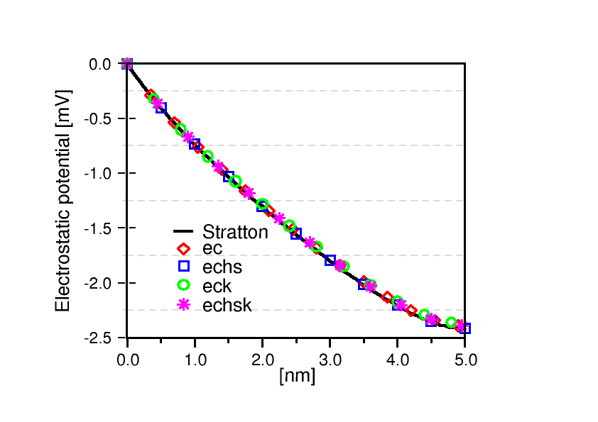
(a) Electrostatic potential

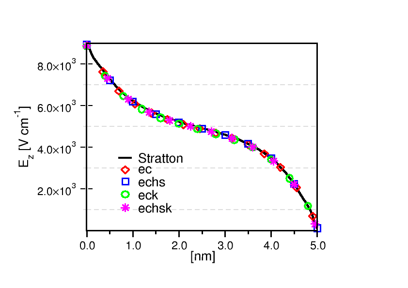
(b) Electric field

Figure 9. Electrical variables along the axis of the channel.

Figures 9(b) and 9(a) show the spatial distributions of the electric potential and of the electric field inside the channel. Since no permanent charge is included in the present simulation, the electric potential (and therefore also the electric field) is determined only by the Coulomb interaction among the ions in the channel. This is the reason why electric field and electric potential distributions are scarcely affected by the different models of Section 4. Figure 9(b) also shows that the electric field profile is monotonic inside the channel. This means, on one hand, that ions are transported with a constant direction depending on their sign (from the intracellular to the extracellular sides in the case of cations, from the extracellular to the intracellular sides in the case of anions), and, on the other hand, that ions cannot be trapped inside the channel, rather they are helped travel throughout the channel. The electrostatic potential shown in Figure 9(a) allows us to perform a first significant model comparison with experimental data reported in Table 2 where the measured value of the transepithelial membrane potential $V_{m}:=\varphi(0)-\varphi(L_{ch})$ is reported for various animals. Results indicate that for all model choices of Section 4, the simulated potential difference is in very good agreement with the data for monkeys [9] which can be considered as the animal species most similar to humans.

$V_{m}\;[\mathrm{mV}]$	Animal	Reference
$3.80\pm 0.26$	ox	[10]
$5.53\pm 0.41$	ox	[11]
$3.83\pm 0.16$	rabbit	[11]
$-3.7\pm 0.3$	toad	[53]
$-1.2\pm 0.1$	rabbit	[30]
$-1.35\pm 0.08$	dog	[21]
$\boxed{-2.5\pm 0.2}$	monkey	[9]

Table 2. Experimental measurements for the transepithelial membrane potential. The boxed value is the measured data for monkeys and is considered as the reference for comparison with our model simulations.

6.2.2. Chemical variables

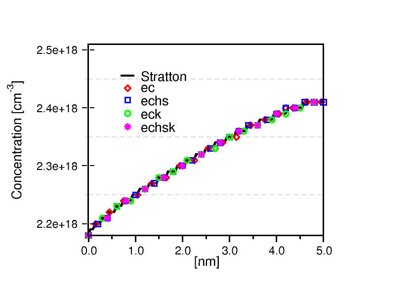
(a) Spatial distribution of K⁺.

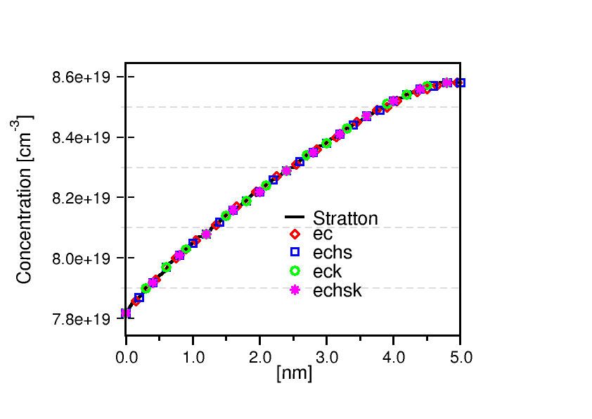
(b) Spatial distribution of Na⁺.

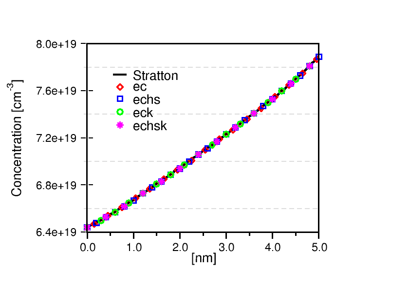
(c) Spatial distribution of Cl^-.

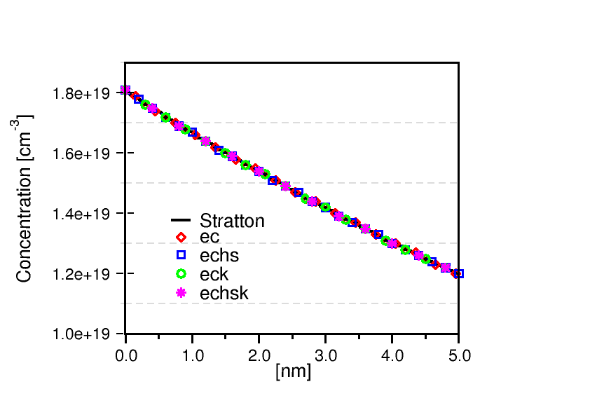
(d) Spatial distribution of HCO${}_{3}^{-}$.

Figure 10. Ionic concentration spatial distribution

Figures 10(a) and 10(b) show the spatial distributions of cations inside the channel whereas Figures 10(c) and 10(d) show the spatial distributions of anions inside the channel. Consistently with the simulated electric field and potential distributions, results indicate that the different models of the volume force density scarcely affect the ionic concentrations indicating that the difference in fluid velocity, shown in the next section, are not strong enough to modify the ionic profiles. As a second comment, we see that the spatial distribution of each ionic concentration is not linear inside the channel because of the presence of the electric field that is responsible for the drift contribution in the ion flux constitutive relation (1b). The data reported in Table 3 allow us to perform a second significant model comparison with experimental data. The data include the computed value of the axial component of the potassium current density at the extracellular side of the channel $Z=L_{ch}$ and the computed value of the axial component of the sodium current density at the intracellular side of the channel $Z=0$ for the various choices for the model of the volume force density $\underline{F}_{ion}$ illustrated in Section 4. To allow a quantitative verification of the biophysical correctness of the predicted exchange of potassium and sodium ions across the channel, we introduce the following parameter

(16) $$r:=\dfrac{g_{\textrm{K}^{+}}}{g_{\textrm{Na}^{+}}},$$

where $g_{\textrm{K}^{+}}$ denotes the boundary value of the flux density of potassium ions that enter into the cell and $g_{\textrm{Na}^{+}}$ denotes the boundary value of the flux density of sodium ions that flow out of the cell. According to the data of Table 12, we have $r=2:3$. The above parameter expresses the biophysical consistency of the boundary data adopted in the numerical simulation because it coincides with the theoretically expected stoichiometric ratio of the K⁺ and Na⁺ ions exchanged ($2:3$) by the sodium-potassium pump as represented in the schematic picture of Figure 3. Because of the continuum approach employed in our model, we are going to check the correct functionality of the simulated pump by computing the following parameter

(17) $$\mathcal{R}:=\Big{|}\dfrac{J_{Z,\textrm{K}^{+}}}{J_{Z,\textrm{Na}^{+}}}\Big{|},$$

where $J_{Z,\textrm{K}^{+}}$ is the potassium ionic current density at the extracellular side of the channel and $J_{Z,\textrm{Na}^{+}}$ is the sodium ionic current density at the intracellular side of the channel. The parameter $\mathcal{R}$ is the counterpart of the quantity $r$ defined in (16) and is quite sensitive to the choice of the volumetric force. As a first comment, the results of Table 3 show that for each considered model of $\underline{F}_{ion}$ the computed potassium current density is negative whereas the computed sodium current density is positive. This is consistent with the physiological function of the sodium-potassium pump because sodium ions flow out of the cell and potassium ions flow into the cell. As a second comment, the computed values of $\mathcal{R}$ indicate that agreement with the theoretical expected ratio 2:3 is achieved only in the case of the Stratton model and of the eck model, whereas the values of $\mathcal{R}$ computed with the other models are not in a feasible range. This allows us to conclude that the VE-PNP model predicts a correct direction of ion flow for the sodium-potassium pump in a good quantitative agreement with the stoichiometric ratio of the pump only if the Stratton or the eck model are adopted to mathematically represent the volume force density in the linear momentum balance equation for the aqueous intracellular fluid.

Model for $\underline{F}_{ion}$	$J_{Z,\textrm{K}^{+}}[\mathrm{Acm^{-2}}]$	$J_{Z,\textrm{Na}^{+}}[\mathrm{Acm^{-2}}]$	$\mathcal{R}$
Stratton	$-0.064$	$0.098$	$\boxed{0.653}$
ec	$-0.054$	$0.44$	$0.123$
echs	$-0.046$	$0.74$	$0.062$
eck	$-0.064$	$0.085$	$\boxed{0.753}$
echsk	$-0.056$	$0.38$	$0.147$

Table 3. Computed values of the axial component of the current density for sodium and potassium. The value $J_{Z,\textrm{K}^{+}}$ is computed at $Z=L_{ch}$ whereas the value $J_{Z,\textrm{Na}^{+}}$ is computed at $Z=0$. We set $\mathcal{R}:=|J_{Z,\textrm{K}^{+}}/J_{Z,\textrm{Na}^{+}}|$. The boxed values indicate the best model predictions to be compared with the theoretical expected ratio 2:3.

6.2.3. Fluid variables

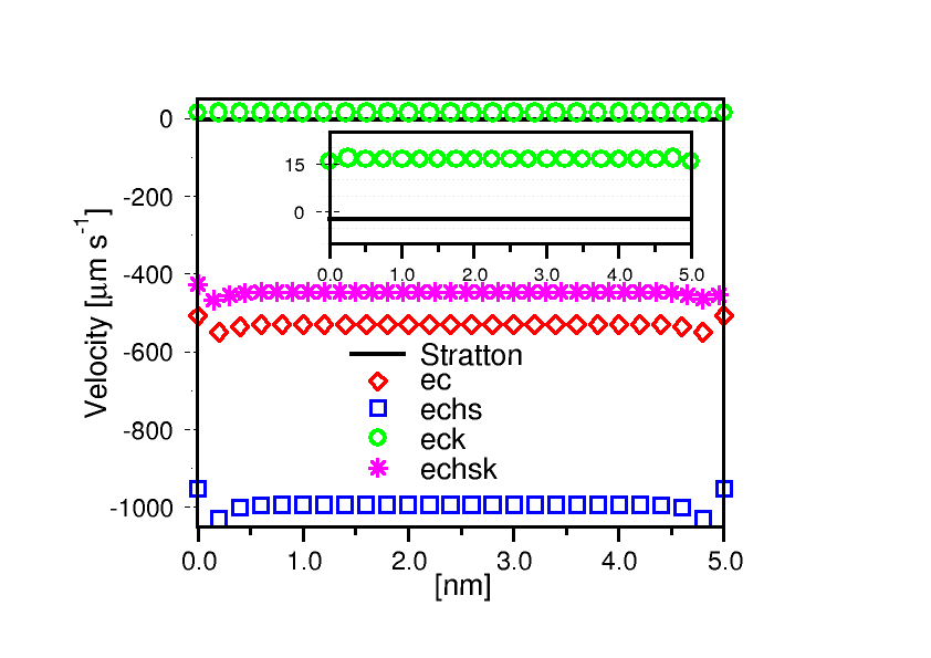
(a) Aqueous humor fluid velocity

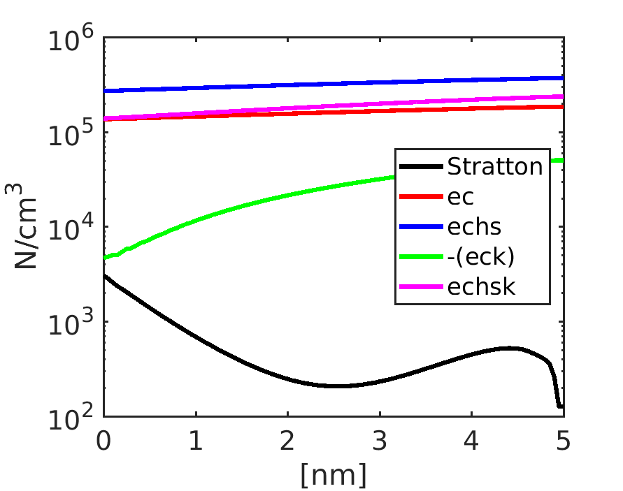
(b) Volumetric force density

Figure 11. Fluid variables along the axis of the channel.

Figures 11(a) and 11(b) show the spatial distributions of the component of the fluid velocity and of the volumetric force density along the $Z$ axis. Predicted velocities are all negative except in the case of the eck model; similarly, the computed volumetric force densities are all positive except in the case of the eck model (in Fig. 11(b) we have reported the absolute value of the force density). Moreover it is easy to check that the variation of the velocity is one-to-one correlated with the variation of the volumetric force density because of the homogeneous initial and boundary conditions that are applied to the Stokes system.

Model for $\underline{F}_{ion}$	$\bar{v}_{Z}[\mathrm{\mu m\;s^{-1}}]$
Stratton	$-2.34$
ec	$-529.5$
echs	$-992$
eck	$\boxed{16.54}$
echsk	$-445.6$

Table 4. Computed mean values of the axial component of the intrachannel water fluid velocity. The boxed value indicates the sole model results that are in agreement with an outflux of aqueous humor from the cell into the extracellular side.

Table 4 reports the values of the fluid velocity computed at the center of the channel for each model considered in Section 4. Results allow us to perform a third significant model comparison with experimental data: only by describing the volume force density through the eck model the VE-PNP formulation is able to predict a positive fluid velocity which corresponds to the production of AH from the cell into the basolateral space. More specifically, if we assume a value of $2.5[\mathrm{\mu l\,s^{-1}}]$ for a normal AH flow through the eye pupil (cf. [35]) and an equivalent radius of $1[\mathrm{mm}]$ for the eye pupil of an adult, we see that a physiological value of $v_{Z}$ is of about $14[\mathrm{\mu m\,s^{-1}}]$ which agrees well with the value of $16.54[\mathrm{\mu m\,s^{-1}}]$ predicted by the eck model. The other results from Table 4 (negative velocities) indicate that the magnitude of the predicted AH flow is nonphysically large, except in the case of the Stratton model, thus justifying its wide adoption in the literature.

6.3. Conclusions

The study of the interaction between the ionic component (Na⁺-K⁺ pump) and AH production through a mathematical continuum approach based on the VE-PNP model, under the condition of adopting the eck formulation of the volume force density that constitutes the source term in the fluid momentum balance equation, shows that simulation results are in agreement with:

1. the experimentally measured value of transepithelial membrane potential;

2. the physiological stoichiometric rate of 2:3 that characterizes the sodium-potassium pump;

3. the direction of current densities of sodium (flowing out of the cell) and potassium (flowing into the cell);

4. the direction of AH flow (outward the cell);

5. the magnitude of AH fluid velocity.

The aferomentioned results support the mathematical and biophysical motivation to adopt the eck model in the remainder of the article where we introduce a more realistic geometrical description of the ionic channel and we include the main ionic pumps to describe the electric pressure exerted by the ions on the intrachannel fluid.

7. Cellular scale simulation of ionic pumps in AH production

In this section we use the VE-PNP model to carry out an extensive quantitative investigation on the active role of the ionic exchanges that are identified in [29] and [28] as important determinants in AH secretion. To this purpose, we adopt the VE-PNP formulation in which the volumetric force exerted from ions onto the fluid is described by the eck model illustrated in Section eck: . In addition, we employ in the numerical simulations a more realistic ionic channel geometry than that shown in Figure 8, obtained by including in the computational domain a small amount of cell membrane as well as the presence of the antichambers. The unified modeling and computational framework is here applied to study the function of each ionic pump illustrated in Section 2 with the goal of examining the output results, such as electrostatic potential, stoichiometric ratios and AH velocity, as functions of the input parameters, such as the osmotic coefficient, the value of the permanent electric charge density and the non-homogeneous Neumann boundary conditions for ion flux densities.

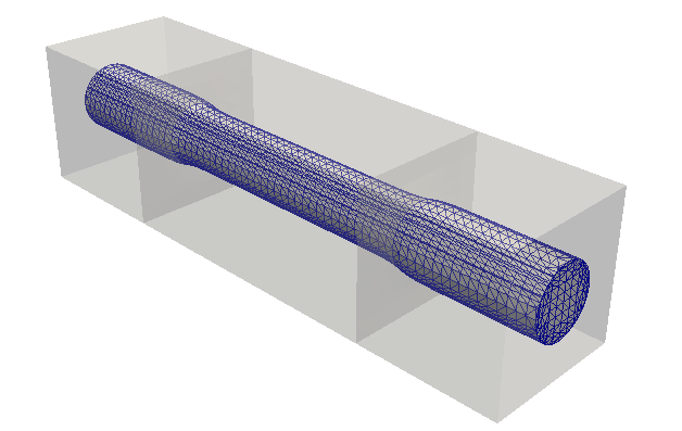
Figure 12. Computational domain for the simulation of the ionic pumps and channels involved in AH production. The two external cylinders represent the channel antichambers whereas the central cylinder is the channel region. The partition of the channel domain into about 110391 tetrahedral elements is illustrated, whereas the mesh partition of the region surrounding the channel is not shown for visual clarity.

Figure 12 shows the geometrical structure constituting the computational domain. The parallelepiped containing the cylinder represents the regions in which the transmembrane channel is divided, namely two external cylinders representing the channel antichambers and a central cylinder representing the ionic channel. The parallelepiped is composed by the union of two cubes of side equal to $2.5[\mathrm{nm}]$ and by a central parallelepiped of length equal to $5[\mathrm{nm}]$ in such a way that the total length is equal to $10[\mathrm{nm}]$. The portion of the cylindrical structure inside the two external cubes has a radius of $0.6[\mathrm{nm}]$ whereas the portion inside the central parallelepiped has a radius of $0.4[\mathrm{nm}]$. The adopted geometrical representation is based on the biophysical setting analyzed in [8, 7] and aims at reproducing the morphology of a realistic protein membrane channel, where the two external cylinders play the role of channel antichambers and the cylinder at the center plays the role of the channel region in which the main electrochemical and fluid processes take place. The full domain has been partitioned in tetrahedral as reported in Figure 12 where the discretization of the parallelepiped surrounding the cylinder is not shown for sake of visual clarity. Referring to the notation of Figure 13, in the remainder of the section, the VE-PNP equations (1a)- (1b) and the Stokes system  (1f)- (1i) are solved only inside the cylinder $\Omega_{INT}$ whereas the Poisson equation (1c)- (1e)) is solved in the whole domain $\Omega$.

7.1. Boundary and initial conditions

In Section 6 we have highlighted the fundamental role played by the BCs in the simulation of the sodium-potassium pump. Because here we are treating a wider variety of ion exchangers, a more complex computational domain as well as the presence of a larger number of ion species, to help the clarity of the discussion we report in Figure 13 a two-dimensional cross-section of the channel geometry and identify the various regions of the domain with the corresponding labels for further reference.

Figure 13. Two-dimensional cross-section of the channel geometry and boundary labels for the simulation of AH production.

7.1.1. Poisson equation

Because of the presence of the interface between the internal cylinder and the surrounding parallelepiped we need to treat the jump of the electric displacement across that interface as well as the possible presence of electrical charge on this interface. Let $\gamma:=\Gamma_{LAT_{INT}^{sideA}}\cup\Gamma_{LAT_{INT}^{sideB}}\cup\Gamma_{LAT_{INT}}$ denote the two-dimensional surface separating the channel region from the surrounding membrane region as depicted in Figure 13. For a given vector-valued function $\underline{\tau}:\Omega\rightarrow\mathbb{R}^{3}$ we define the jump of $\underline{\tau}$ across the surface $\gamma$ as

$$\,[\![\underline{\tau}]\!]_{\gamma}:=\left(\underline{\tau}|_{\Omega\setminus\Omega_{INT}}|_{\gamma}-\underline{\tau}|_{\Omega_{INT}}|_{\gamma}\right)\cdot\underline{n},$$

whereas for a given scalar-valued function $\phi:\Omega\rightarrow\mathbb{R}$ we define the jump of $\phi$ across the surface $\gamma$ as

$$\,[\![\phi]\!]_{\gamma}:=\phi|_{\Omega\setminus\Omega_{INT}}|_{\gamma}\underline{n}-\phi|_{\Omega_{INT}}|_{\gamma}\underline{n}.$$

We notice that the jump of a vector-valued function is a scalar function whereas the jump of a scalar-valued function is a vector function. For all $t\in I_{T}$, the BCs for the Poisson equation (1c)-(1e) are:

(18a) $$\varphi=0 \qquad\textrm{on }sideA_{int}$$

(18b) $$\underline{D}\cdot\underline{n}=0 \qquad\textrm{on }\Gamma_{LAT}\cup sideB\cup sideA\cup sideB_{int}$$

(18c) $$\,[\![\underline{D}]\!]_{\gamma}=h_{\gamma} \qquad\textrm{on }\gamma$$

(18d) $$\,[\![\varphi]\!]_{\gamma}=0 \qquad\textrm{on }\gamma,$$

where:

$$h_{\gamma}=\left\{\begin{array}[]{ll}\sigma_{fixed}&\qquad\textrm{on }\Gamma_{LAT_{INT}}\\ 0&\qquad\textrm{on }\Gamma_{LAT_{INT}^{sideA}}\cup\Gamma_{LAT_{INT}^{sideB}},\end{array}\right.$$

$\sigma_{fixed}$ $[\mathrm{C\;m^{-2}}]$ being a given distribution of superficial permanent charge density that mathematically represents the electric charge contained in the aminoacid structure of the protein surrounding the ion channel. We notice that the interface condition (18d) expresses the physical fact that the electric potential is a continuous function across $\gamma$, whereas the interface condition (18c) expresses the physical fact that the normal component of the displacement vector is discontinuous across the surface separating the channel region and the lipid membrane bilayer because of the presence of aminoacid fixed charge density $\sigma_{fixed}$. The value of $\sigma_{fixed}$ needs be determined in order to reproduce the correct functionality of the several ionic pumps/exchangers. To this purpose, a simulation campaign has to be performed to heuristically tune-up the values of $\sigma_{fixed}$ (see [43] for the sodium-potassium pump). The results of this procedure in the present context are reported in Table 5.

Pump/channel	$\sigma_{fixed}[\mathrm{C\;cm^{-2}}]$
sodium-potassium pump	$-1\cdot 10^{10}$
calcium-sodium pump	$-1.2\cdot 10^{12}$
anion channel	$+3.9\cdot 10^{11}$
hydrogenate-sodium pump	$-2.65\cdot 10^{12}$

Table 5. Values of the fixed charge density $\sigma_{fixed}$.

7.1.2. Nernst-Planck equations

The several ionic pumps/exchangers involved in AH production are simulated by considering the contribution of different ions in order to produce the correct electrostatic potential drop across the cell membrane. The list of these ions is reported below. In complete analogy with what done in Section 6 for the BCs and ICs of the Nernst-Planck equations (1a)- (1b), we report in Tables 6- 9 the BCs and ICs adopted to reproduce the correct biophysical functionality of each ion pump.

Na⁺-K⁺ pump:

: Na⁺, K⁺, Cl^-, HCO${}_{3}^{-}$ are treated.

Ca⁺⁺-Na⁺ pump:

: Na⁺, K⁺, Cl^-, HCO${}_{3}^{-}$, Ca⁺⁺ are treated.

Cl^--HCO${}_{3}^{-}$ pump:

: Na⁺, K⁺, Cl^-, HCO${}_{3}^{-}$ are treated.

H⁺-Na⁺ pump:

: Na⁺, K⁺, Cl^-, HCO${}_{3}^{-}$, H⁺ are treated.

Na+ = Na${}^{+}_{in}$	$\underline{f}_{\textrm{K}^{+}}\cdot\underline{n}=g_{\textrm{K}^{+}}$	on $sideA_{int}$
K+ = K${}^{+}_{out}$	$\underline{f}_{\textrm{Na}^{+}}\cdot\underline{n}=g_{\textrm{Na}^{+}}$	on $sideB_{int}$
$\underline{f}_{\textrm{Na}^{+}}\cdot\underline{n}=0$	$\underline{f}_{\textrm{K}^{+}}\cdot\underline{n}=0$	on $\gamma$
K${}^{+^{0}}(x)=$ K${}^{+}_{0}$	Na${}^{+^{0}}(x)=$ Na${}^{+}_{0}$	in $\Omega_{INT}$
Cl${}^{-}=$ Cl${}^{-}_{in}$	HCO${}_{3}^{-}=$ HCO${}^{-}_{3_{in}}$	on $sideA_{int}$
Cl${}^{-}=$ Cl${}^{-}_{out}$	HCO${}_{3}^{-}=$ HCO${}^{-}_{3_{out}}$	on $sideB_{int}$
$\underline{f}_{\textrm{Cl}^{-}}\cdot\underline{n}=0$	$\underline{f}_{\textrm{HCO}_{3}^{-}}\cdot\underline{n}=0$	on $\gamma$
Cl${}^{-^{0}}(x)=$ Cl${}^{-}_{0}$	HCO${}_{3}^{-^{0}}(x)=$ HCO${}_{3_{0}}^{-}$	in $\Omega_{INT}$

Table 6. BCs and ICs for the sodium-potassium pump.

K${}^{+}=$ K${}^{+}_{in}$	Na${}^{+}=$ Na${}^{+}_{in}$	$\underline{f}_{\textrm{Ca}^{++}}\cdot\underline{n}=g_{\textrm{Ca}^{++}}$	on $sideA_{int}$
K${}^{+}=$ K${}^{+}_{out}$	Ca${}^{++}=$ Ca${}^{++}_{out}$	$\underline{f}_{\textrm{Na}^{+}}\cdot\underline{n}=g_{\textrm{Na}^{+}}$	on $sideB_{int}$
$\underline{f}_{\textrm{Ca}^{++}}\cdot\underline{n}=0$	$\underline{f}_{\textrm{Na}^{+}}\cdot\underline{n}=0$	$\underline{f}_{\textrm{K}^{+}}\cdot\underline{n}=0$	on $\gamma$
K${}^{+^{0}}(x)=$ K${}^{+}_{0}$	Na${}^{+^{0}}(x)=$ Na${}^{+}_{0}$	Ca${}^{{++}^{0}}(x)=$ Ca${}^{++}_{0}$	in $\Omega_{INT}$
Cl${}^{-}=$ Cl${}^{-}_{in}$	HCO${}_{3}^{-}=$ HCO${}^{-}_{3_{in}}$		on $sideA_{int}$
Cl${}^{-}=$ Cl${}^{-}_{out}$	HCO${}_{3}^{-}=$ HCO${}^{-}_{3_{out}}$		on $sideB_{int}$
$\underline{f}_{\textrm{Cl}^{-}}\cdot\underline{n}=0$	$\underline{f}_{\textrm{HCO}_{3}^{-}}\cdot\underline{n}=0$		on $\gamma$
Cl${}^{-^{0}}(x)=$ Cl${}^{-}_{0}$	HCO${}_{3}^{-^{0}}(x)=$ HCO${}_{3_{0}}^{-}$		in $\Omega_{INT}$

Table 7. BCs and ICs for the calcium-sodium pump.

K${}^{+}=$ K${}^{+}_{in}$	Na${}^{+}=$ Na${}^{+}_{in}$	on $sideA_{int}$
K${}^{+}=$ K${}^{+}_{out}$	Na${}^{+}=$ Na${}^{+}_{out}$	on $sideB_{int}$
$\underline{f}_{\textrm{Na}^{+}}\cdot\underline{n}=0$	$\underline{f}_{\textrm{K}^{+}}\cdot\underline{n}=0$	on $\gamma$
K${}^{+^{0}}(x)=$ K${}^{+}_{0}$	Na${}^{+^{0}}(x)=$ Na${}^{+}_{0}$	in $\Omega_{INT}$
$\underline{f}_{\textrm{Cl}^{-}}\cdot\underline{n}=g_{\textrm{Cl}^{-}}$	$\underline{f}_{\textrm{HCO}_{3}^{-}}\cdot\underline{n}=g_{\textrm{HCO}_{3}^{-}}$	on $sideA_{int}$
Cl${}^{-}=$ Cl${}^{-}_{out}$	HCO${}_{3}^{-}=$ HCO${}^{-}_{3_{out}}$	on $sideB_{int}$
$\underline{f}_{\textrm{Cl}^{-}}\cdot\underline{n}=0$	$\underline{f}_{\textrm{HCO}_{3}^{-}}\cdot\underline{n}=0$	on $\gamma$
Cl${}^{-^{0}}(x)=$ Cl${}^{-}_{0}$	HCO${}_{3}^{-^{0}}(x)=$ HCO${}_{3_{0}}^{-}$	in $\Omega_{INT}$

Table 8. BCs and ICs for the anion channel.

K${}^{+}=$ K${}^{+}_{in}$	Na${}^{+}=$ Na${}^{+}_{in}$	$\underline{f}_{\textrm{H}^{+}}\cdot\underline{n}=g_{\textrm{H}^{+}}$	on $sideA_{int}$
K${}^{+}=$ K${}^{+}_{out}$	H${}^{+}=$ H${}^{+}_{out}$	$\underline{f}_{\textrm{Na}^{+}}\cdot\underline{n}=g_{\textrm{Na}^{+}}$	on $sideB_{int}$
$\underline{f}_{\textrm{H}^{+}}\cdot\underline{n}=0$	$\underline{f}_{\textrm{Na}^{+}}\cdot\underline{n}=0$	$\underline{f}_{\textrm{K}^{+}}\cdot\underline{n}=0$	on $\gamma$
K${}^{+^{0}}(x)=$ K${}^{+}_{0}$	Na${}^{+^{0}}(x)=$ Na${}^{+}_{0}$	H${}^{+^{0}}(x)=$ H${}^{+}_{0}$	in $\Omega_{INT}$
Cl${}^{-}=$ Cl${}^{-}_{in}$	HCO${}_{3}^{-}=$ HCO${}^{-}_{3_{in}}$		on $sideA_{int}$
Cl${}^{-}=$ Cl${}^{-}_{out}$	HCO${}_{3}^{-}=$ HCO${}^{-}_{3_{out}}$		on $sideB_{int}$
$\underline{f}_{\textrm{Cl}^{-}}\cdot\underline{n}=0$	$\underline{f}_{\textrm{HCO}_{3}^{-}}\cdot\underline{n}=0$		on $\gamma$
Cl${}^{-^{0}}(x)=$ Cl${}^{-}_{0}$	HCO${}_{3}^{-^{0}}(x)=$ HCO${}_{3_{0}}^{-}$		in $\Omega_{INT}$

Table 9. BCs and ICs for the hydrogenate-sodium pump.

The values of the boundary data for the ionic pumps and ionic channels are specified in Tables 14- 17.

7.1.3. Stokes system

We adopt the same BCs and ICs as in Section 6:,

(19a) $$\underline{u}=\underline{0} \qquad\textrm{on }\gamma$$

(19b) $$\underline{\underline{{\sigma}}}\>\underline{n}=\underline{0} \qquad\textrm{on }sideA_{int}\cup sideB_{int}$$

(19c) $$\underline{u}(\underline{x},0)=\underline{0} \qquad\forall\underline{x}\in\Omega_{INT}.$$

As already pointed out, to describe the volumetric force at the right-hand side of the linear momentum balance equation in the Stokes system we use the eck model. The value of $k$ is considered a characteristic property of the single pump and channel and is reported in Table 10.

Pump/channel	$k[\mathrm{N\;m}]$
sodium-potassium pump	$4.1\cdot 10^{-19}$
calcium-sodium pump	$24\cdot 10^{-19}$
anion channel	$4.1\cdot 10^{-19}$
hydrogenate-sodium pump	$4\cdot 10^{-19}$

Table 10. Values of the electrochemical osmotic parameter $k$ for each pump/channel involved in the process of AH production.

7.2. Simulation results

Reported data for the vector-valued variables (such as electric field, current densities and velocity) are the $Z$ component of the vectors because the other two computed components were comparably negligible. We set $t_{0}=0\;[\mathrm{s}]$ and $T_{obs}=50\;[\mathrm{ns}]$, a sufficiently large value to ensure that the simulated system has reached steady-state conditions at $t=T_{obs}$: all the figures in the remainder of the section illustrate computed results at this time. The values of the dielectric permittivity of the intrachannel fluid $\epsilon_{r}^{f}$, of the fluid shear viscosity $\mu_{f}$, of the fluid mass density $\rho_{f}$ and of the diffusion coefficients $D_{i}$ of each $i$-th ionic species involved in the computational tests are reported in Table 1.

7.2.1. Electrical variables

(a) Electrostatic potential

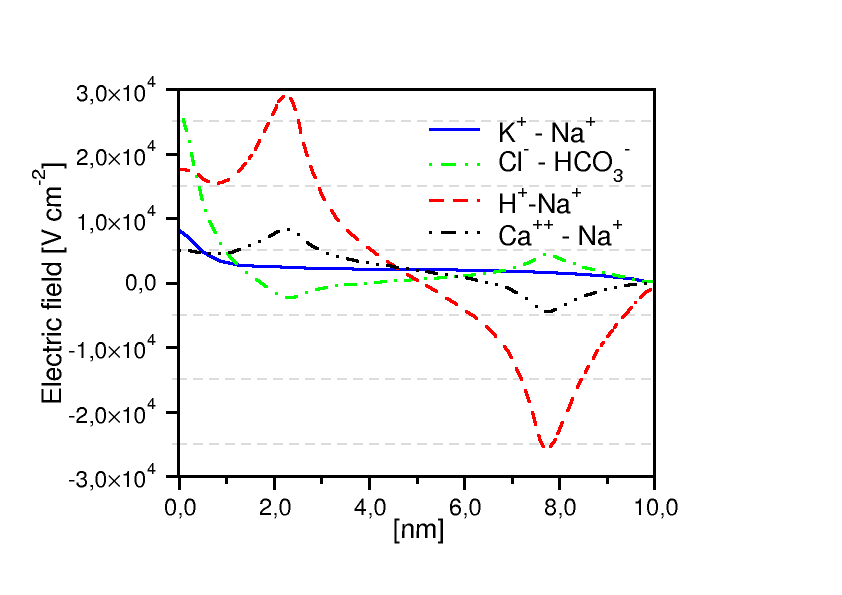
(b) Electric field

Figure 14. Electrical variables along the axis of the channel.

Figure 14(a) shows the transepithelial electrostatic potential as calculated by the simulations. We note how the electric potential is strongly influenced by the presence of the fixed surface charge density $\sigma_{fixed}$ in the central region of the domain (cf. Table 5), with particular emphasis in the case of the hydrogenate-sodium pump. It is remarkable to notice that, as in the case of the simulation of the sodium-potassium pump illustrated in Section 6, also in this more complex biophysical setting, for each simulated pump/channel, the computed value of the transepithelial membrane potential is in very good agreement with the experimental data for monkeys reported in Table 2.

Figure 14(b) shows the computed spatial behavior of the axial component $E_{Z}$ of the electric field for each considered pump/channel. Consistently with electrostatic potential, we see that in all simulations $E_{Z}$ is a monotonically function of position in the central region of the channel. Then, coming closer to the outlet section at $Z=L_{ch}$, all the simulated profiles become flat in accordance with the homogeneous Neumann boundary condition (18b). Specifically, in the case of cation pumps, the electric field is decreasing along the central part of the channel whereas in the case of the anion channel the electric field is increasing. These two opposite behaviors are related to the presence of surface charge on $\Gamma_{LAT_{IN}}$ of opposite sign (negative for cation pumps, positive for the anion pump). In the case of the hydrogenate-sodium pump, the electric field profile experiences a large increase in magnitude moving along the channel axis from the intracellular side towards the extracellular side because of the elevated negative fixed charge density distributed on the lateral surface on the channel region (cf. Table 5).

7.2.2. Chemical variables

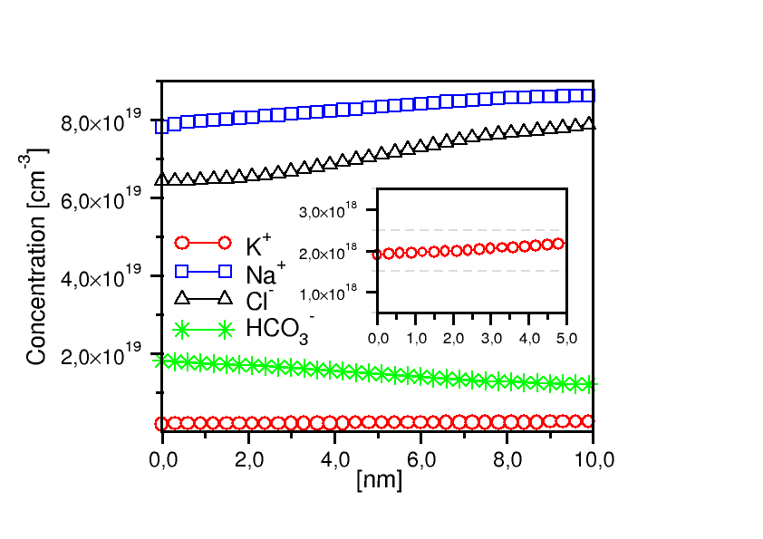
(a) Sodium-potassium pump.

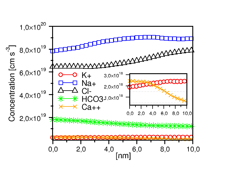
(b) Calcium-sodium pump.

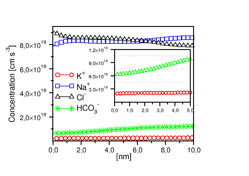
(c) Anion channel.

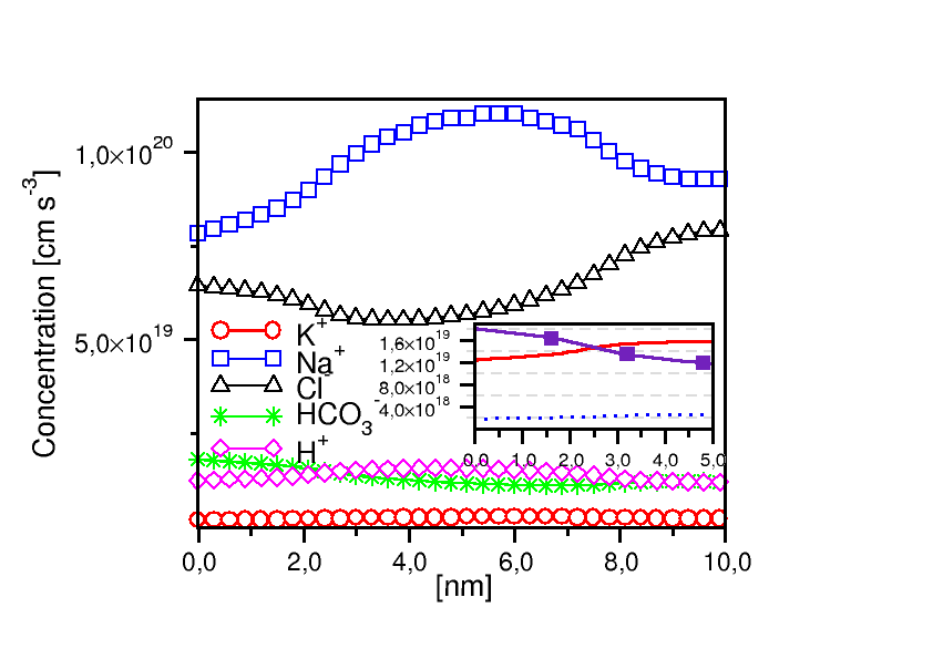
(d) Hydrogenate-sodium pump.

Figure 15. Computed ionic concentration along the $Z$ axis

The computed profiles of the ion concentrations for each simulated ionic pump and channel are reported in Figures 15(a)- 15(d). Results show the onset of a concentration gradient for each simulated ion species which appears not to be spatially constant for all ion species because of the action of the electric drift force which displaces the ion profile from the linear equilibrium distribution corresponding to a null electric field. Particularly worth noticing is the occurrence of significant variations for the concentration of the sodium ion in the simulation of the hydrogenate-sodium pump shown in Figure 15(d). These variations are the result of the attractive electrostatic force exerted on the sodium ions by the elevated negative fixed charge density distributed on the lateral surface on the channel region (cf. Table 5).

Figures 16(a)- 16(d) show the spatial distributions of the computed axial component of the ionic current density for each pump and channel. For sake of clarity, in these figures we report only the current density related to the pump/exchanger functionality. We notice that for each ion, the value of the current density along the $Z$ axis is not constant because the cross-section varies along the channel axis.

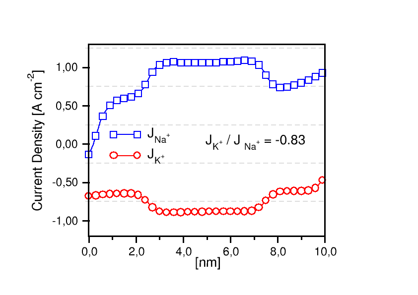
(a) Sodium-potassium pump.

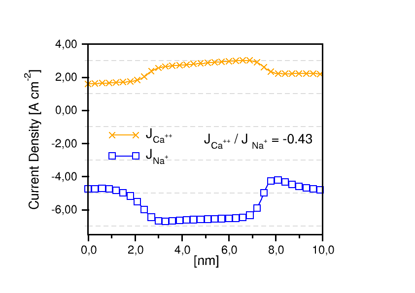
(b) Calcium-sodium pump.

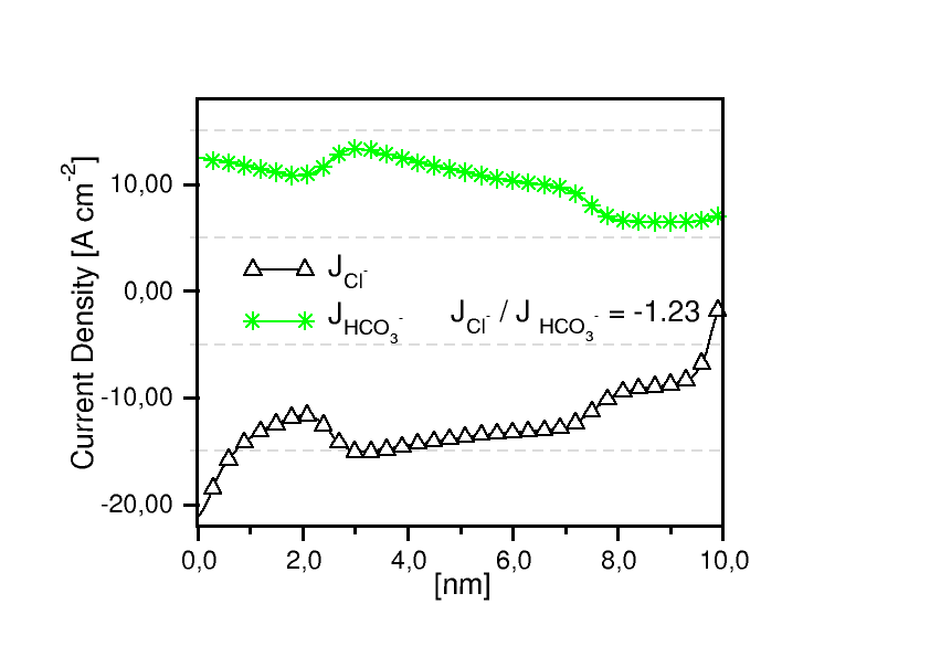
(c) Anion channel.

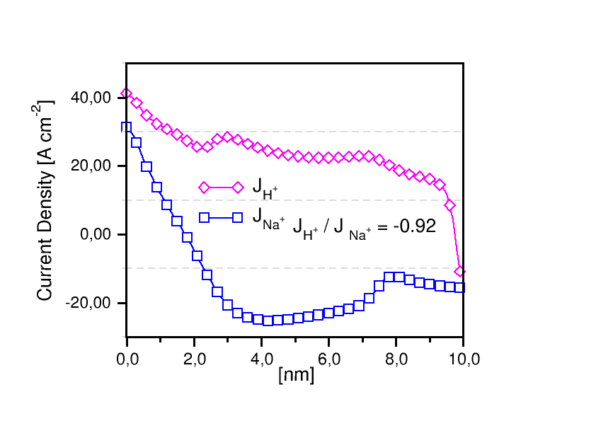
(d) Hydrogenate-sodium pump.

Figure 16. Computed ionic current density along the $Z$ axis

Firstly, the sign of the computed current density for each simulated pump agrees with the theoretically expected direction. As a second comment, the predicted values of the stoichiometric ratio $\mathcal{R}$ reasonably agrees with the corresponding theoretical value $r$. Specifically, in the case of the sodium-potassium pump shown in Figure 16(a), $\mathcal{R}=0.83$, whereas $r=2:3=0.67$, in the case of the calcium-sodium pump shown in Figure 16(b), $\mathcal{R}=0.43$ whereas $r=1:3=0.33$, in the case of the anion channel shown in Figure 16(c) we have $\mathcal{R}=1.23$ to be compared with $r=1:1$ and in the case of the hydrogenate-sodium pump shown in Figure 16(d)) the value $\mathcal{R}=0.92$ fairly well agrees with the theoretical value $r=1:1$.

7.2.3. Fluid variables

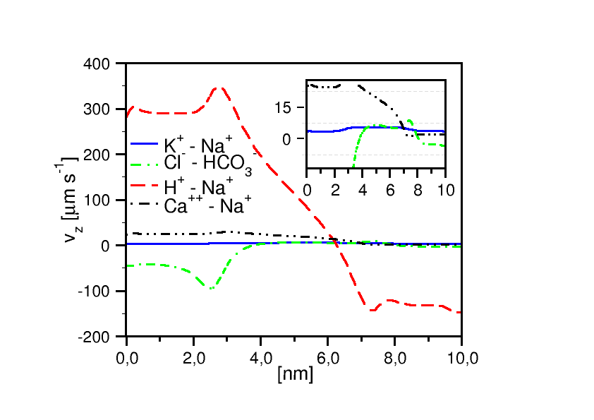
Figure 17. Computed spatial distribution of the axial component of fluid velocity for each pump/channel involved in AH production.

Figure 17 shows the spatial distribution of the axial component of the intrachannel water fluid velocity predicted by the simulation with the VE-PNP model of each ionic pump and channel involved in the process of AH production. Results exhibit a significant difference among the various pumps mainly due to the presence of the fixed surface charge density $\sigma_{fixed}$ in the central region of the domain that needed to be included to reproduce the correct pump functionalities. Specifically, in the case of the cation-based ionic pumps, model simulation predicts a positive value of the velocity in the whole computational domain whereas in the case of the anion channel the computed AH fluid velocity is strictly positive only in the central region of the domain. In the case of the hydrogenate-sodium pump, the elevated fixed surface charge density on $\Gamma_{LAT_{INT}}$ gives rise to a change of sign of the axial component of the electric field at about the center of the domain. This, in turn, reflects into a change of sign in the volume force density $\underline{F}_{ion}$ in the momentum balance equation of the fluid, causing an inversion of the intrachannel fluid flow at $Z=7.5[\mathrm{nm}]$ where the direction of the axial velocity changes sign, from positive to negative. These results seem to suggest that the main ionic pump/exchangers contributing to AH secretion are those that actively involve Na⁺.

Figure 18 shows an example of three-dimensional computed spatial distribution of the fluid velocity in the case of the calcium-sodium pump. Results clearly show that AH flows from the intracellular space towards the extracellular space.

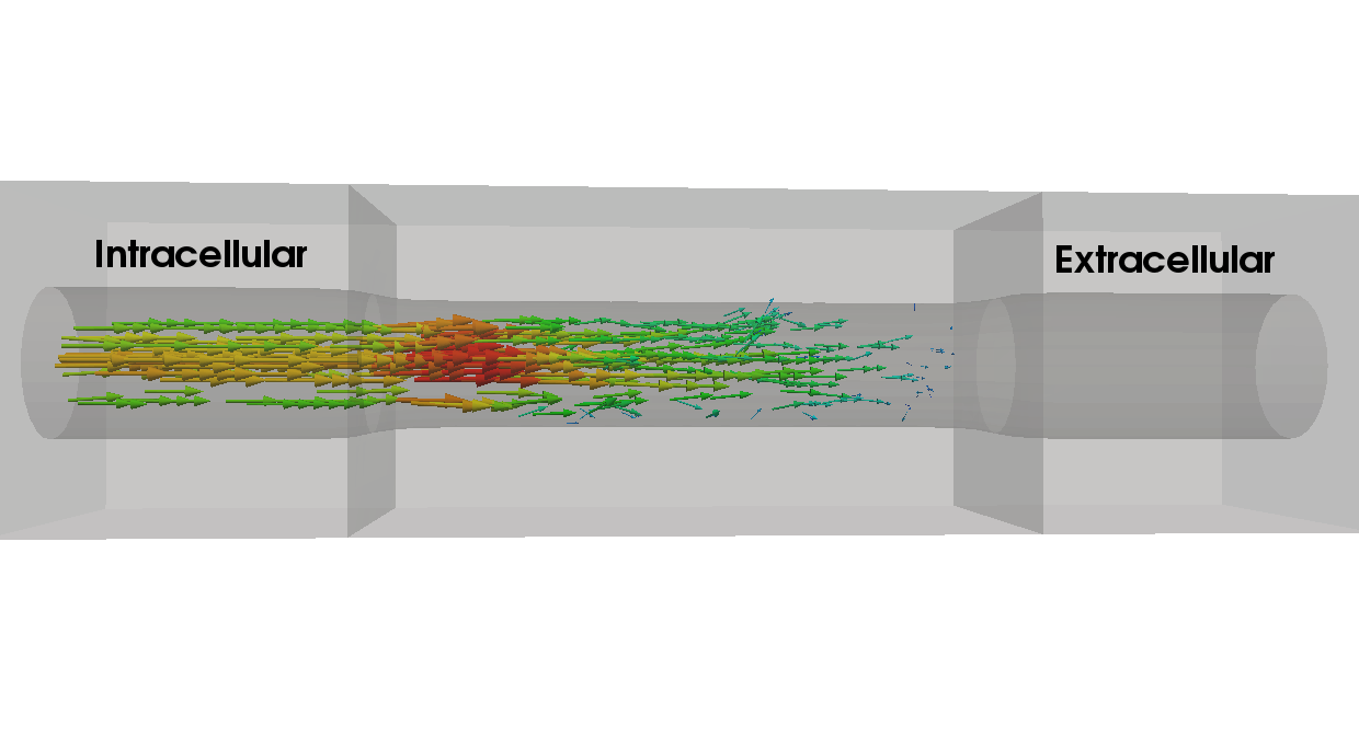
Figure 18. Computed three-dimensional spatial distribution of fluid velocity in the case of the calcium-sodium pump.

7.2.4. Further remarks on pump functionality

In this section we briefly address a series of further considerations on the analysis of the simulation of the various ionic pumps and channels involved in the process of AH production, in particular, those related to pump/exchanger functionality. The first consideration concerns the temporal evolution of calcium in the Ca⁺⁺-Na⁺ pump. To this purpose, Figure 19(a) illustrates the spatial calcium concentration at $t=0$ (dashed line) and that at $t=T_{obs}$ (solid line). Results show a decrease of the level of calcium in the intracellular side of the domain. Such a decrease is slow because of the relatively low value $D_{\textrm{Ca}^{++}}=7.92\cdot 10^{-6}\;[\mathrm{cm^{2}s^{-1}}]$ of the diffusion coefficient adopted in the numerical simulation but, nonetheless, agrees with the theoretical expectation that physiological intracellular calcium level should be very low in healthy conditions (see [2, 13]).

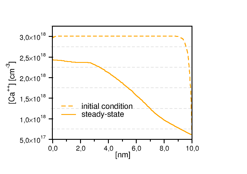
(a) [Ca⁺⁺] in the calcium-sodium pump.

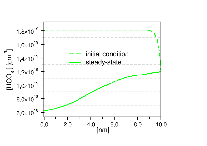
(b) [HCO${}_{3}^{-}$] for the anion channel.

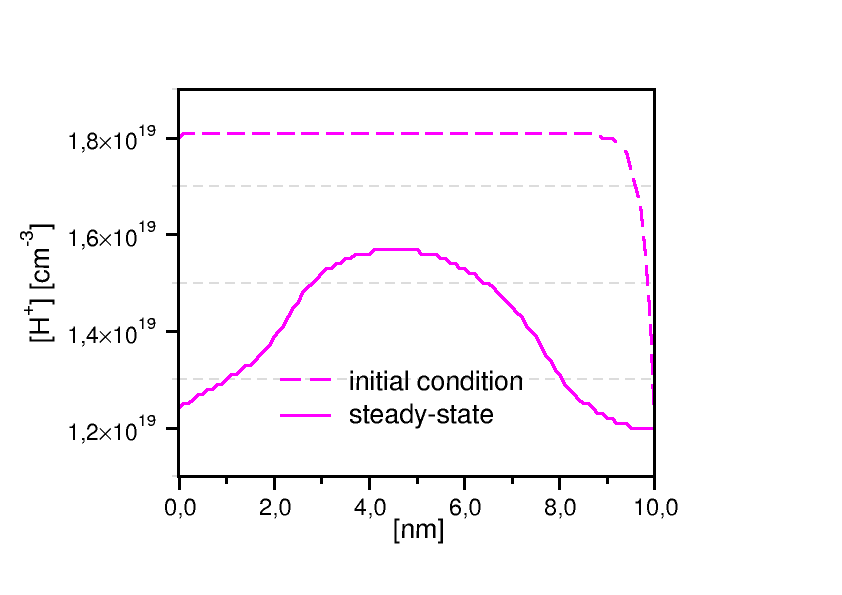
(c) [H⁺] for the hydrogenate-sodium pump

Figure 19. Computed ionic current density along the $Z$ axis t various time: Dashed line: distribution at $t=0$. Solid line: distribution at $t=T_{obs}$

The second consideration concerns the time behavior of carbonate (HCO${}_{3}^{-}$) in the anion channel. To this purpose, Figure 19(b) illustrates the spatial carbonate concentration at $t=0$ (dashed line) and that at $t=T_{obs}$ (solid line). Results show a significant decrease of the level of carbonate in the intracellular region. This behavior agrees with the fact that the simulated electric field profile for the anion channel is positive in the intracellular region of the domain (cf. Figure 14(b)) and therefore carbonate ions are swept away from left to right. For further analysis of the importance of the carbonate ion in AH production, we refer to [34].

The third consideration concerns the spatial distribution of hydrogenate (H⁺) in the simulation of the hydrogenate-sodium pump. To this purpose, Figure 19(c) illustrates the spatial carbonate profile at $t=0$ (dashed line) and that at $t=T_{obs}$ (solid line). Similarly to the previous case of carbonate, results show a significant reduction with simulation time of hydrogenate concentration in all the domain. However, unlike the previous case, concentration reduction equally occurs in both intracellular and extracellular sides whereas hydrogenate accumulation occurs in the channel region. This behavior is due to the direction of the electric field (cf. Figure 14(b)) which pushes H⁺ from left to right in the intracellular side (where $E_{Z}>0$) and from right to left in the extracellular side (where $E_{Z}<0$).

7.3. Summary of the simulation results

In Table 11 we report the main outcomes of the simulation of ionic pumps and channels carried out in the context of AH secretion induced at the cellular scale level by the effect of ionic pressure exerted on transmembrane fluid. To summarize: a unified modeling and computational framework allowed us to successfully simulate the functionality of several ionic pump/exchangers while preserving at the same time the features of each single exchanger, by a proper selection of the ion flux density BCs, of the osmotic gradient coefficient and of the amount of aminoacid charge in the channel protein folder. These conclusions are significant outcomes of our computational model because osmotic gradient coefficient and permanent electric surface charge do not have yet a quantitative comparison with experimental data, though, they have been shown to be essential parts of the biophysical description of the channel and to play a relevant role in determining AH flow direction.

Pump	$k[\mathrm{N\,cm}]$	$\sigma_{fixed}[\mathrm{Ccm^{-2}}]$	$\varphi_{m}[\mathrm{mV}]$	$\mathcal{R}$	$v_{Z}[\mathrm{\mu m\;s^{-1}}]$
K+ - Na+	$4.1\cdot 10^{-19}$	$-1.0\cdot 10^{10}$	$-2.67$	$0.83(0.67)$	$[4,\;5.56]$
Cl- - HCO${}_{3}^{-}$	$24\cdot 10^{-19}$	$+3.9\cdot 10^{11}$	$-2.46$	$1.23(1)$	$[-100,\;+6.56]$
H+ - Na+	$4.0\cdot 10^{-19}$	$-2.65\cdot 10^{12}$	$-2.49$	$0.92(1)$	$[-150,\;300]$
Ca++ - Na+	$3.95\cdot 10^{-19}$	$-6\cdot 10^{11}$	$-2.39$	$0.43(0.33)$	$[2,\;28]$

Table 11. A summary of the simulation results for ionic pumps and channel involved in AH production. Aside the predicted value of $\mathcal{R}$ we report in braces the theoretically expected value. The column $v_{Z}$ reports for each row the predicted range of the fluid velocity.

8. Conclusions, model limitations and future objectives

A unified modeling and computational framework with electrochemical osmotic correction and with a realistic geometry to represent the computational domain, has been proposed to investigate the main functional principles of the sodium-potassium pump, the calcium-sodium pump, the anion channel and the hydrogenate-sodium pump, that are involved in the production of aqueoud humor in the ciliary body of the eye. The theoretical model has been demonstrated to correctly reproduce, for each simulated ionic pump and channel, existing experimental data of transepithelial membrane potential in animal models. The model has also allowed, for the first time to the best of our knowledge in the study of AH production, the quantitative analysis of novel biophysical mechanisms such as the physiological stoichiometric rate, the direction of AH flow and the magnitude of AH fluid velocity. Thus, the present study motivates the further development of this modeling approach to (i) simulate the simultaneous presence and action of the several ionic pump/exchangers considered in this work, with the aim of quantitatively estimating their reciprocal influence; (ii) include the presence of other molecules actively transported through the cell membrane, including the ascorbic acid, which is secreted by a transporter (Sodium-dependent vitamin C transporter 2 (SVCT2)) [52]; and (iii) the simulation of the effect of administration of a drug in the regulation of AH secretion.

It is expected that such theoretical advancement of the frontier of knowledge in this branch of Human Sciences may significantly help design new molecules for drug synthesis and, as a consequence, considerably reduce time and costs for clinical availability of new pharmacological therapies.

It is important to emphasize, though, that a number of biophysical limitations still affect the proposed mathematical model of aqueous humor dynamics. Among them, we mention that our model does not account for (i) autonomic system pathways, specifically, the sympathetic and parasympathetic (see [51]); (ii) variations due to the circadian rhythm (see [48]); (iii) the role of aquaporins in the exchange of fluid across the cell membrane (see [44]). A research effort to address these limitations is currently in progress.

Data tables

K${}^{+}_{0}$	$g_{\textrm{K}^{+}}$	K${}^{+}_{out}$
$2.41\cdot 10^{18}\;[\mathrm{cm^{-3}}]$	$+4\cdot 10^{17}\;[\mathrm{cm^{-2}s^{-1}}]$	$2.41\cdot 10^{18}\;[\mathrm{cm^{-3}}]$
Na${}^{+}_{0}$	Na${}^{+}_{in}$	$g_{\textrm{Na}^{+}}$
$8.19\cdot 10^{19}\;[\mathrm{cm^{-3}}]$	$7.82\cdot 10^{19}\;[\mathrm{cm^{-3}}]$	$+6\cdot 10^{17}\;[\mathrm{cm^{-2}s^{-1}}]$

Table 12. Boundary and initial data for the cations in Sec. 6.

Cl${}^{-}_{0}$	Cl${}^{-}_{in}$	Cl${}^{-}_{out}$
$7.17\cdot 10^{19}\;[\mathrm{cm^{-3}}]$	$6.44\cdot 10^{19}\;[\mathrm{cm^{-3}}]$	$7.89\cdot 10^{19}\;[\mathrm{cm^{-3}}]$
HCO${}^{-}_{3,0}$	HCO${}^{-}_{3,in}$	HCO${}^{-}_{3,out}$
$1.51\cdot 10^{19}\;[\mathrm{cm^{-3}}]$	$1.81\cdot 10^{19}\;[\mathrm{cm^{-3}}]$	$1.2\cdot 10^{19}\;[\mathrm{cm^{-3}}]$

Table 13. Boundary and initial data for the anions in Sec. 6.

K${}^{+}_{0}$ $[\mathrm{cm^{-3}}]$	$g_{\textrm{K}^{+}}$ $[\mathrm{cm^{-2}s^{-1}}]$	K${}^{+}_{out}$ $[\mathrm{cm^{-3}}]$
$2.41\cdot 10^{18}$	$-4\cdot 10^{19}$	$2.41\cdot 10^{18}$
Na${}^{+}_{0}$ $[\mathrm{cm^{-3}}]$	Na${}^{+}_{in}$ $[\mathrm{cm^{-3}}]$	$g_{\textrm{Na}^{+}}$ $[\mathrm{cm^{-2}s^{-1}}]$
$8.19\cdot 10^{19}$	$7.82\cdot 10^{19}$	$-6\cdot 10^{19}$
Cl${}^{-}_{0}$ $[\mathrm{cm^{-3}}]$	Cl${}^{-}_{in}$ $[\mathrm{cm^{-3}}]$	Cl${}^{-}_{out}$ $[\mathrm{cm^{-3}}]$
$7.17\cdot 10^{19}$	$6.44\cdot 10^{19}$	$7.89\cdot 10^{19}$
HCO${}_{3}^{-}$0 $[\mathrm{cm^{-3}}]$	HCO${}_{3}^{-}$in $[\mathrm{cm^{-3}}]$	HCO${}_{3}^{-}$out $[\mathrm{cm^{-3}}]$
$1.51\cdot 10^{19}$	$1.81\cdot 10^{19}$	$1.20\cdot 10^{19}$

Table 14. Data for the sodium-potassium pump in Sec. 7.

K${}^{+}_{0}$ $[\mathrm{cm^{-3}}]$	K${}^{+}_{in}$ $[\mathrm{cm^{-3}}]$	K${}^{+}_{out}$ $[\mathrm{cm^{-3}}]$
$2.41\cdot 10^{18}$	$1.90\cdot 10^{18}$	$2.41\cdot 10^{18}$
Na${}^{+}_{0}$ $[\mathrm{cm^{-3}}]$	Na${}^{+}_{in}$ $[\mathrm{cm^{-3}}]$	$g_{\textrm{Na}^{+}}$ $[\mathrm{cm^{-2}s^{-1}}]$
$8.19\cdot 10^{19}$	$7.82\cdot 10^{19}$	$6\cdot 10^{19}$
Ca${}^{++}_{0}$ $[\mathrm{cm^{-3}}]$	$g_{\textrm{Ca}^{++}}$ $[\mathrm{cm^{-2}s^{-1}}]$	Ca${}^{++}_{out}$ $[\mathrm{cm^{-3}}]$
$3.011\cdot 10^{18}$	$2\cdot 10^{19}$	$6.022\cdot 10^{17}$
Cl${}^{-}_{0}$ $[\mathrm{cm^{-3}}]$	Cl${}^{-}_{in}$ $[\mathrm{cm^{-3}}]$	Cl${}^{-}_{out}$ $[\mathrm{cm^{-3}}]$
$7.17\cdot 10^{19}$	$6.44\cdot 10^{19}$	$7.89\cdot 10^{19}$
HCO${}_{3}^{-}$0 $[\mathrm{cm^{-3}}]$	HCO${}_{3}^{-}$in $[\mathrm{cm^{-3}}]$	HCO${}_{3}^{-}$out $[\mathrm{cm^{-3}}]$
$1.51\cdot 10^{19}$	$1.81\cdot 10^{19}$	$1.2\cdot 10^{19}$

Table 15. Data for the calcium-sodium pump in Sec. 7.

K${}^{+}_{0}$ $[\mathrm{cm^{-3}}]$	K+in $[\mathrm{cm^{-3}}]$	K+out $[\mathrm{cm^{-3}}]$
$2.41\cdot 10^{18}$	$1.90\cdot 10^{18}$	$2.41\cdot 10^{18}$
Na${}^{+}_{0}$ $[\mathrm{cm^{-3}}]$	Na${}^{+}_{in}$ $[\mathrm{cm^{-3}}]$	Na+out $[\mathrm{cm^{-3}}]$
$8.19\cdot 10^{19}$	$7.82\cdot 10^{19}$	$8.55\cdot 10^{19}$
Cl-0 $[\mathrm{cm^{-3}}]$	$g_{\textrm{Cl}^{-}}$ $[\mathrm{cm^{-2}s^{-1}}]$	Cl-out $[\mathrm{cm^{-3}}]$
$7.17\cdot 10^{19}$	$8\cdot 10^{19}$	$7.89\cdot 10^{19}$
HCO${}_{3}^{-}$0 $[\mathrm{cm^{-3}}]$	$g_{\textrm{HCO}_{3}^{-}}$ $[\mathrm{cm^{-2}s^{-1}}]$	HCO${}_{3}^{-}$out $[\mathrm{cm^{-3}}]$
$1.81\cdot 10^{19}$	$-8\cdot 10^{19}$	$1.20\cdot 10^{19}$

Table 16. Data for the anion channel in Sec. 7.

K${}^{+}_{0}$ $[\mathrm{cm^{-3}}]$	K${}^{+}_{in}$ $[\mathrm{cm^{-3}}]$	$K^{+}_{out}$ $[\mathrm{cm^{-3}}]$
$2.41\cdot 10^{18}$	$1.90\cdot 10^{18}$	$2.41\cdot 10^{18}$
Na${}^{+}_{0}$ $[\mathrm{cm^{-3}}]$	Na${}^{+}_{in}$ $[\mathrm{cm^{-3}}]$	$g_{\textrm{Na}^{+}}$ $[\mathrm{cm^{-2}s^{-1}}]$
$8.19\cdot 10^{19}$	$7.82\cdot 10^{19}$	$1.0\cdot 10^{20}$
H${}^{+}_{0}$ $[\mathrm{cm^{-3}}]$	$g_{\textrm{H}^{+}}$ $[\mathrm{cm^{-2}s^{-1}}]$	H${}^{+}_{out}$ $[\mathrm{cm^{-3}}]$
$1.81\cdot 10^{19}$	$1.0\cdot 10^{20}$	$1.20\cdot 10^{19}$
Cl${}^{-}_{0}$ $[\mathrm{cm^{-3}}]$	Cl${}^{-}_{in}$ $[\mathrm{cm^{-3}}]$	Cl${}^{-}_{out}$ $[\mathrm{cm^{-3}}]$
$7.17\cdot 10^{19}$	$6.44\cdot 10^{19}$	$7.89\cdot 10^{19}$
HCO${}_{3}^{-}$0 $[\mathrm{cm^{-3}}]$	HCO${}_{3}^{-}$in $[\mathrm{cm^{-3}}]$	HCO${}_{3}^{-}$out $[\mathrm{cm^{-3}}]$
$1.81\cdot 10^{19}$	$1.81\cdot 10^{19}$	$1.20\cdot 10^{19}$

Table 17. Data for the hydrogenate-sodium pump in Sec. 7.

References

- [1] P. Airoldi, A. G. Mauri, R. Sacco, and J. W. Jerome. Three-dimensional numerical simulation of ion nanochannels. Journal of Coupled Systems and Multiscale Dynamics, 3(1):57–65, 2015.
- [2] B. Alberts. Molecular Biology of the Cell, 5th Ed. Garland Science, 2008.
- [3] M. Z. Bazant. Encyclopedia of Microfluidics and Nanofluidics, chapter Part 14: Nonlinear electrokinetic phenomena, pages 1461–1470. Springer, Berlin, Heidelberg, New York, 2008.
- [4] M. Z. Bazant. Electrokinetics meets electrohydrodynamics. J. Fluid Mech., 782:1–4, 2015.
- [5] C. Breitkopf and K. Swider-Lyons. Springer Handbook of Electrochemical Energy. Springer Handbooks. Springer Berlin Heidelberg, 2016.
- [6] R. F. Brubaker. The Glaucomas, chapter Measurement of aqueous humor flow by fluorophotometry, pages 337–344. Mosby, S. Louis, 1989.
- [7] D. P. Chen and R. S. Eisenberg. Charges, currents, and potentials in ionic channels of one conformation. Biophysical journal, 64(5):1405–1421, 1993.
- [8] D. P. Chen and R. S. Eisenberg. Flux, coupling, and selectivity in ionic channels of one conformation. Biophysical journal, 65:727–746, 1993.
- [9] T. C. Chu, O. A. Candia, and S. M. Podos. Electrical parameters of the isolated monkey ciliary epithelium and effects of pharmacological agents. Invest Ophthalmol Vis Sci, 28(10):1644–1648, 1987.
- [10] D. F. Cole. Electrical potential across the isolated ciliary body observed in vitro. Br J Ophthalmol, 45(10):641–653, 1961.
- [11] D. F. Cole. Electrical potential across the isolated ciliary body of ox and rabbit. Br J Ophthalmol, 46(10):577–591, 1962.
- [12] B. Eisenberg, Y. Hyon, and C. Liu. Energy variational analysis of ions in water and channels: Field theory for primitive models of complex ionic fluids. The Journal of Chemical Physics, 133(10):104104, 2010.
- [13] G. Bard Ermentrout and David H. Terman. Mathematical Foundations of Neuroscience. Springer, 1st edition. edition, 2010.
- [14] B.T. Gabelt and P.L. Kaufman. Adler’s physiology of the eye, volume 8, chapter Aqueous humour hydrodynamics, pages 237–289. Mosby, S. Louis, 1995.
- [15] M. Goel, R.G. Piccianni, R.K. Lee, and S.K. Bhattacharya. Aqueous humour dynamics: a review. Open Ophthalmol J., 4:52–59, 2010.
- [16] B. Goldhagen, A. D. Proia, D. L. Epstein, and P. V. Rao. Elevated levels of rhoa in the optic nerve head of human eyes with glaucoma. Journal of glaucoma, 21(8):530–538, 2012.
- [17] G. Guidoboni, A. Harris, J. C. Arciero, B. A. Siesky, A. Amireskandari, A. L. Gerber A. H. Huck, N. J. Kim, S. Cassani, and L. Carichino. Mathematical modeling approaches in the study of glaucoma disparities among people of african and european descents. J. Coupled Syst. Multiscale Dyn., 1(1):1–21, 2013.
- [18] A. Heijl, M. C. Leske, B. Bengtsson, L. Hyman, B. Bengtsson, and M. Hussein. Reduction of intraocular pressure and glaucoma progression: results from the early manifest glaucoma trial. Archives of ophthalmology, 120(10):1268–1279, 2002.
- [19] B. Hille. Ionic Channels of Excitable Membranes. Sinauer Associates, Inc., Sunderland, MA, 2001.
- [20] M. Honjo, H. Tanihara, M. Inatani, N. Kido, T. Sawamura, B. Y. J. T. Yue, S. Narumiya, and Y. Honda. Effects of rho-associated protein kinase inhibitor y-27632 on intraocular pressure and outflow facility. Investigative ophthalmology & visual science, 42(1):137–144, 2001.
- [21] S. Iizuka, K. Kishida, S. Tsuboi, K. Emi, and R. Manabe. Electrical characteristics of the isolated dog ciliary body. Curr Eye Res, 3(3):417–421, 1984.
- [22] M. Jaeger, M. Carin, M. Medale, and G. Tryggvason. The osmotic migration of cells in a solute gradient. Biophysical Journal, 77(3):1257 – 1267, 1999.
- [23] J. W. Jerome. Analytical approaches to charge transport in a moving medium. Transport Theory and Statistical Physics, 31:333–366, 2002.
- [24] J. W. Jerome and R. Sacco. Global weak solutions for an incompressible charged fluid with multi-scale couplings: Initial-boundary value problem. Nonlinear Analysis, 71:e2487–e2497, 2009.
- [25] G. E. Karniadakis, A. Beskok, and N. Aluru. Microflows and Nanoflows: Fundamentals and Simulation. Interdisciplinary Applied Mathematics. Springer-Verlag New York, 2005.
- [26] J. P. Keener and J. Sneyd. Mathematical Physiology. Springer, New York, 1998.
- [27] J. W. Kiel. Physiology of the intraocular pressure. In J. Feher, editor, Pathophysiology of the Eye, number 4 in Glaucoma, pages 79–107. Akademiai Kiadò, Budapest, 1998.
- [28] J.W. Kiel, M. Hollingsworth, R. Rao, M. Chen, and H.A. Reitsamer. Ciliary blood flow and aqueous humour production. Prog Retin Eye Res., 30:1–17, 2011.
- [29] J.W. Kiel, H.A. Reitsamer, J.S. Walker, and F.W. Kiel. Effects of nitric oxide synthase inhibition on ciliary blood flow, aqueous production and intraocular pressure. Exp Eye Res., 73:355–364, 2001.
- [30] T. Krupin, P. S. Reinach, O. A. Candia, and S. M. Podos. Transepithelial electrical measurements on the isolated rabbit iris-ciliary body. Exp Eye Res., 38:115–123, 1984.
- [31] H.H. Mark. Aqueous humor dynamics in historical perspective. Surv Ophthalmol., 55:89–100, 2010.
- [32] A. G. Mauri, A. Bortolossi, G. Novielli, and R. Sacco. 3d finite element modeling and simulation of industrial semiconductor devices including impact ionization. Journal of Mathematics in Industry, 5(1):1, Mar 2015.
- [33] A. G. Mauri, R. Sacco, and M. Verri. Electro-thermo-chemical computational models for 3d heterogeneous semiconductor device simulation. Applied Mathematical Modelling, 39(14):4057 – 4074, 2015.
- [34] A.G. Mauri, L. Sala, P. Airoldi, G. Novielli, R. Sacco, S. Cassani, G. Guidoboni, B. Siesky, and A. Harris. Electro-fluid dynamics of aqueous humor production: simulations and new directions. Journal for Modeling in Ophthalmology, 2:48–58, 2016.
- [35] R. Moses. Intraocular pressure. In R. Moses and W. Hart, editors, Adler’s Physiology of the Eye: Clinical Application, pages 223–245. C. V. Mosby Co., St Louis, 1987.
- [36] H. A. Quigley and A. T. Broman. The number of people with glaucoma worldwide in 2010 and 2020. British Journal of Ophthalmology, 90(3):262–267, 2006.
- [37] P. V. Rao and D. L. Epstein. Rho gtpase/rho kinase inhibition as a novel target for the treatment of glaucoma. BioDrugs, 21(3):167–177, 2007.
- [38] Y. Rosenfeld. Free-energy model for the inhomogeneous hard-sphere fluid mixture and density-functional theory of freezing. Phys. Rev. Lett., 63:980–983, Aug 1989.
- [39] Y. Rosenfeld, M. Schmidt, H. Lowen, and P. Tarazona. Fundamental-measure free energy density functional theory for hard spheres: Dimensional crossover and freezing. Phys. Rev. E, 55:4245–4263, 1997.
- [40] R. Roth. Introduction to density functional theory of classical systems: Theory and applications. Lecture Notes, November 2006. ITAP, Universitaet Stuttgart and Max-Planck-Institut fur Metallforschung, Stuttgart Germany.
- [41] R. Roth, R. Evans, A. Lang, and G. Kahl. Fundamental measure theory for hard-sphere mixtures revisited: the white bear version. Journal of Physics: Condensed Matter, 14(46):12063, 2002.
- [42] I. Rubinstein. Electrodiffusion of Ions. SIAM, 1990.
- [43] R. Sacco, P. Airoldi, A. G. Mauri, and J. W. Jerome. Three-dimensional simulation of biological ion channels under mechanical, thermal and fluid forces. Applied Mathematical Modelling, 43(Supplement C):221 – 251, 2017.
- [44] K. L. Schey, Z. Wang, and Y. Wenke, J. L. & Qi. Aquaporins in the eye: Expression, function, and roles in ocular disease. Biochimica et Biophysica Acta, 1840(5):1513–1523, 2014.
- [45] M. Schmuck. Analysis of the Navier-Stokes-Nernst-Planck-Poisson system. Mathematical Models and Methods in Applied Sciences, 19(6):993–1015, 2009.
- [46] M. Shahidullah, W.A. Al-Malki, and N.A. Delamare. Mechanism of aqueous humour secretion, its regulation and relevance to glaucoma. In S. Rumelt, editor, Glaucoma - Basic and clinical concepts. INTECH open science, 2011.
- [47] M. B. Shields. A Study Guide for Glaucoma. Williams & Wilkins, 1982.
- [48] A. J. Sit, C. B. Nau, J. W. McLaren, D. H. Johnson, and D. Hodge. Circadian variation of aqueous dynamics in young healthy adults. Investigative Ophthalmology & Visual Science, 49(4):1473–1479, 2008.
- [49] J.A. Stratton, IEEE Antennas, and Propagation Society. Electromagnetic Theory. An IEEE Press classic reissue. Wiley, 2007.
- [50] M. Szopos, S. Cassani, G. Guidoboni, C. Prud’homme, R. Sacco, B. Siesky, and A. Harris. Mathematical modeling of aqueous humor flow and intraocular pressure under uncertainty: towards individualized glaucoma management. Journal for Modeling in Ophthalmology, 1:29–39, 2016.
- [51] C. B. Toris. Encyclopedia of the Eye, 1st Edition, pages 312–315. Academic Press, 2010.
- [52] H. Tsukaguchi, T. Tokui, B. Mackenzie, and et al. A family of mammalian Na+-dependent L-ascorbic acid transporters. Nature, 399:70–75, 1999.
- [53] T. Watanabe and Y. Saito. Characteristics of ion transport across the isolated ciliary epithelium of the toad as studied by electrical measurements. Exp Eye Res, 27(2):215–226, 1978.
- [54] P.J. Wistrand. Carbonic anhydrase in the anterior uvea of the rabbit. Acta Physiol Scand., 24:145–148, 1951.
- [55] A. Wojcik-Gryciuk, M. Skup, and W. Waleszczyk. Glaucoma -state of the art and perspectives on treatment. Restor Neurol Neurosci., 34(1):107–123, 2015.