Homoclinic saddle to saddle-focus transitions in 4D systems

Manu Kalia1, Yuri A. Kuznetsov1,2 and Hil G.E. Meijer1 1 Department of Applied Mathematics, University of Twente, Zilverling Building, P.O. Box 217, 7500AE Enschede, The Netherlands 2 Mathematical Institute, Utrecht University, Budapestlaan 6, 3584CD Utrecht, The Netherlands [M.Kalia, I.A.Kouznetsov, H.G.E.Meijer]@utwente.nl
Abstract

A saddle to saddle-focus homoclinic transition when the stable leading eigenspace is 3-dimensional (called the 3DL bifurcation) is analyzed. Here a pair of complex eigenvalues and a real eigenvalue exchange their position relative to the imaginary axis, giving rise to a 3-dimensional stable leading eigenspace. This transition is different from the standard Belyakov bifurcation, where a double real eigenvalue splits either into a pair of complex-conjugate eigenvalues or two distinct real eigenvalues. In the wild case, we obtain sets of codimension 1 and 2 bifurcation curves and points that asymptotically approach the 3DL bifurcation point and have a structure that differs from that the standard Belyakov case. We also give an example of this bifurcation in the wild case occuring in a perturbed Lorenz-Stenflo 4D ODE model.

1 Introduction

Homoclinic orbits play an important role in the analysis of ODEs depending on parameters

x˙=F(x,α),xn,αm,formulae-sequence˙𝑥𝐹𝑥𝛼formulae-sequence𝑥superscript𝑛𝛼superscript𝑚\dot{x}=F(x,\alpha),\quad x\in\mathbb{R}^{n},\alpha\in\mathbb{R}^{m}, (1)

where F𝐹F is smooth. Orbits homoclinic to hyperbolic equilibria are of specific interest, as they are structurally unstable, and the corresponding parameter values generically belong to codim 1 manifolds in the parameter space msuperscript𝑚\mathbb{R}^{m}. Bifurcations in generic one-parameter families transverse to such manifolds depend crucially on the configuration of leading eigenvalues of the equilibrium, i.e. the stable eigenvalues with largest real part, and the unstable eigenvalues with smallest real part.
Refer to caption
(a) Saddle
Refer to caption
(b) Saddle-focus
Refer to caption
(c) Focus-focus
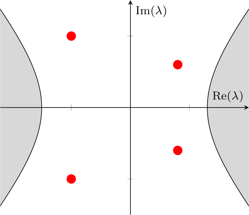
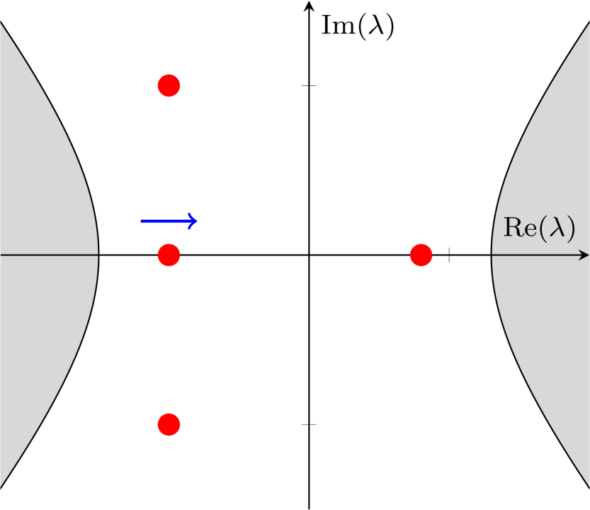
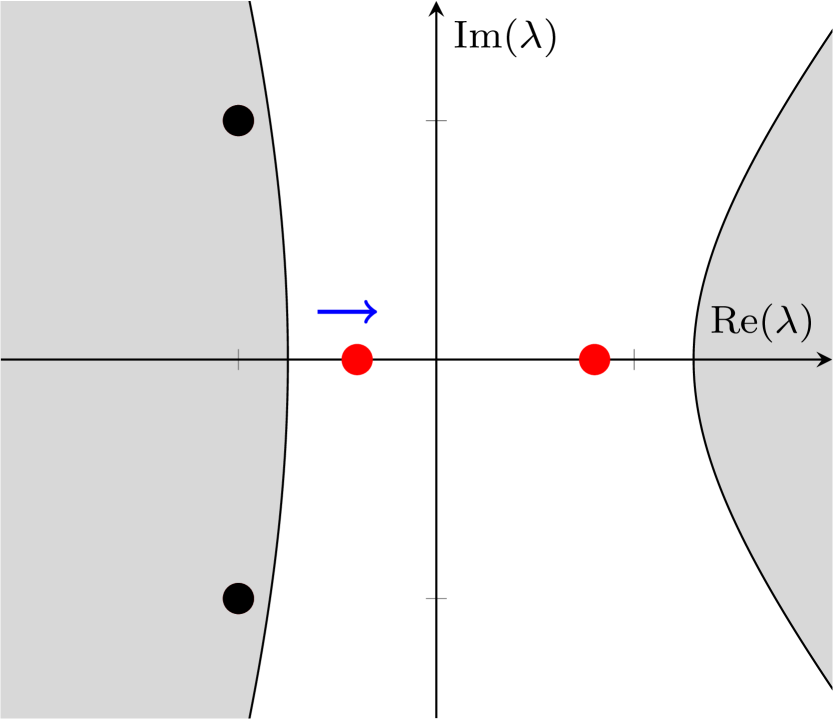
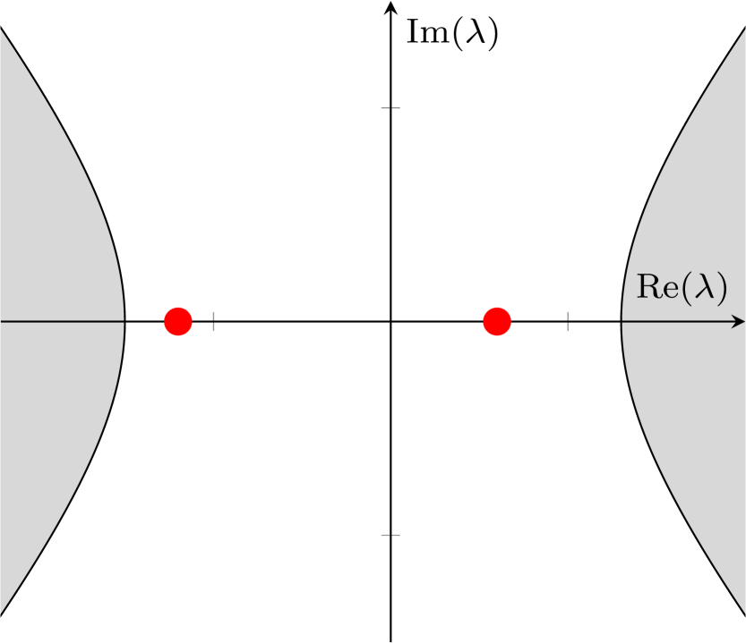
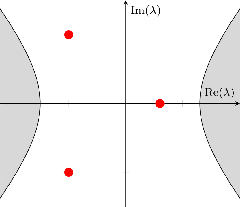
Figure 1: Configurations of leading eigenvalues λ𝜆\lambda (red). Gray area contains all non-leading eigenvalues.

In Figure 1, we see three configurations with simple leading eigenvalues, for which a detailed description of the bifurcations occurring near the homoclinic orbit is available (see, e.g. [1, 2, 3, 4]). For example, in the saddle case, a single periodic orbit appears generically. In the saddle-focus case, we could assume that the leading stable eigenvalues are complex by applying time-reversal if necessary. In this case, infinitely many periodic orbits exist if the saddle quantity σ0subscript𝜎0\sigma_{0}, defined as the sum of the real part of the leading unstable and stable eigenvalues, is positive. This phenomenon is called Shilnikov’s homoclinic chaos [5, 6]. On the contrary, if σ0subscript𝜎0\sigma_{0} is negative, then generically only one periodic orbit appears. Thus, the sign of σ0subscript𝜎0\sigma_{0} distinguishes wild and tame saddle-focus homoclinic cases. Note that in the wild case many other bifurcations occur nearby, including infinite sequences of fold (limit point, LP) and period-doubling (PD) bifurcations of periodic orbits, as well as secondary homoclinic bifurcations, which all accumulate on the primary homoclinic bifurcation manifold [7]. In the focus-focus case, which will not be considered in this paper, homoclinic chaos is always present.

Moving along the primary homoclinic manifold in the parameter space of (1), one may encounter a transition from the saddle case (a) to the saddle-focus case (b). This is a degenerate situation, and the corresponding homoclinic parameter values form generically a codim 2 sub-manifold in the parameter space. Nearby bifurcations should be studied using generic two-parameter families transverse to this codim 2 sub-manifold. We can therefore restrict ourselves to generic two-parameter ODEs (m=2𝑚2m=2), where the primary homoclinic orbit exists along a smooth homoclinic curve in the parameter plane, while the saddle to saddle-focus transition happens at an isolated point on this curve. There are many more codim 2 homoclinic bifurcations, see [8, 3, 4].

As already noted in [8], the simplest saddle to saddle-focus transitions correspond to

  • (i)

    a double leading eigenvalue;

  • (ii)

    three simple leading eigenvalues.
Refer to caption
(a) α<0𝛼0\alpha<0
Refer to caption
(b) α=0𝛼0\alpha=0
Refer to caption
(c) α>0𝛼0\alpha>0
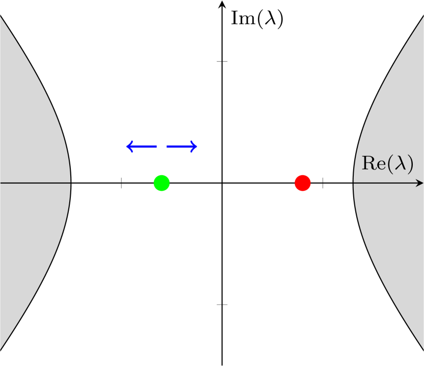
Figure 2: Eigenvalue configurations of the saddle to saddle-focus transition in case (i); α𝛼\alpha is the parameter along the homoclinic curve and the bifurcation occurs at α=0𝛼0\alpha=0. Arrows point in the direction of generic movement of eigenvalues. The green marker indicates a double real eigenvalue. The gray areas contain non-leading eigenvalues, leading eigenvalues are marked red and non-leading eigenvalues are marked black.
Refer to caption
(a) α<0𝛼0\alpha<0
Refer to caption
(b) α=0𝛼0\alpha=0
Refer to caption
(c) α>0𝛼0\alpha>0
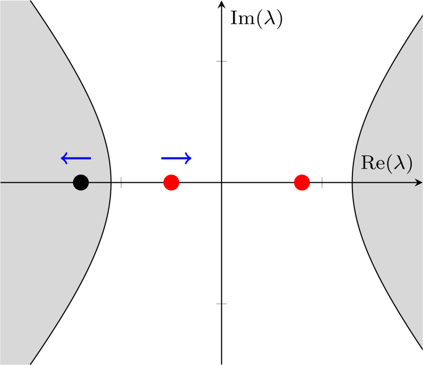
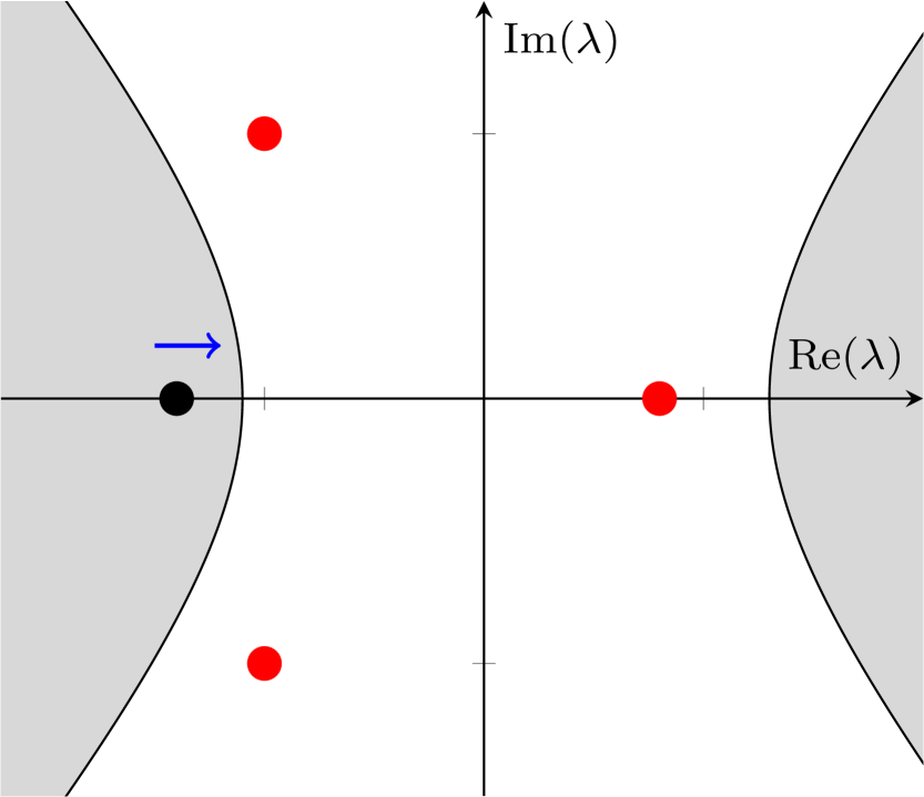
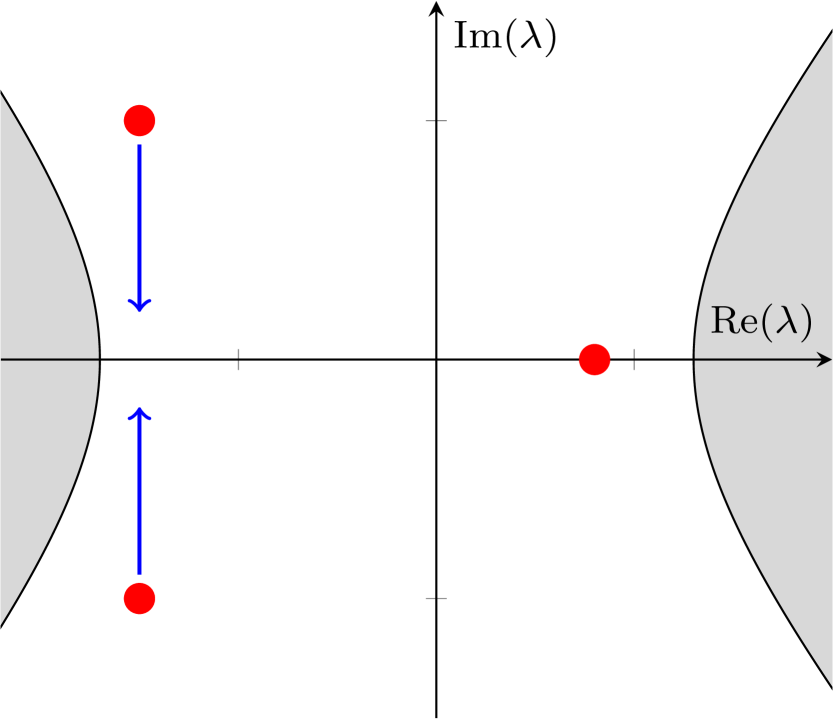
Figure 3: Eigenvalue configurations of the saddle to saddle-focus transition in case (ii); the scalar bifurcation parameter along the homoclinic curve is α𝛼\alpha. Arrows point in the direction of generic movement of eigenvalues. There is a codimension 2 situation at α=0𝛼0\alpha=0, where the leading stable eigenspace becomes 3-dimensional. Non-leading eigenvalues are contained in the gray area, leading eigenvalues are marked red and non-leading eigenvalues are marked black.

In case (i), see Figure 2, the pair of leading complex eigenvalues approaches the real axis and splits into two distinct real eigenvalues. At the transition there is a double real eigenvalue and the leading eigenspace is two-dimensional. In case (ii), see Figure 3, the real eigenvalue exchanges its position with the pair of complex-conjugate eigenvalues. At the transition there are two complex-conjugate eigenvalues and one real eigenvalue with the same real part. All leading eigenvalues are simple and the leading eigenspace is 3-dimensional.

Case (i) is a saddle to saddle-focus homoclinic transition that appears in various applications, e.g. in biophysics [9] and ecology [10]. Moreover, in these applications the transition corresponds to the wild case with σ0>0subscript𝜎00\sigma_{0}>0. This case was first studied theoretically by Belyakov [11], who proved that the corresponding bifurcation diagram is complicated. We call this case the standard Belyakov case. In [11, 10] a description of the main features of the universal bifurcation diagram close to this transition for n=3𝑛3n=3 in the wild case has been obtained:

  1. 1.

    There exists an infinite set of limit point (LP) and period doubling (PD) bifurcation curves.

  2. 2.

    There exists an infinite set of secondary homoclinic curves corresponding to homoclinic orbits making two global excursions and various numbers of local turns near the equilibrium.

  3. 3.

    Both sets have the same ‘bunch’ shape: The corresponding curves emanate from the codim 2 point and accumulate onto the branch of primary saddle-focus homoclinic orbits. The secondary homoclinics accumulate only from one side.

Case (ii) has been observed in [12] for a 4D system of ODEs arising from a study of travelling waves in a neural field model. We note that the transition in [12] is tame with σ0<0subscript𝜎00\sigma_{0}<0. As in the standard Belyakov case, we expect a complicated bifurcation diagram in the wild case, i.e. when σ0>0subscript𝜎00\sigma_{0}>0.

Our paper is devoted to the theoretical analysis of the homoclinic saddle to saddle-focus transition for case (ii), when the leading stable eigenspace is three-dimensional, focusing on the wild case. We call this transition the 3DL-transition. To our best knowledge, no systematic analysis of this case is available in the literature. A possible reason for this gap is that case (ii) could only occur in (1) with n4𝑛4n\geq 4, while case (i) happens already in three-dimensional ODEs. This leads to the study of a three-dimensional return map in case (ii), which is much more difficult to analyze than the planar return map in the standard Belyakov case (i).

For n𝑛n-dimensional systems, generically the analysis of homoclinic bifurcations can be restricted to the Homoclinic Center Manifold, a k𝑘k-dimensional invariant finitely-smooth manifold that is tangent at the equilibrium to the eigenspace corresponding to the union of all leading eigenvalues [13, 14, 15, 16]. Thus, k𝑘k is the number of all leading eigenvalues of the equilibrium, counting their multiplicities. For the saddle to saddle-focus homoclinic transition case (ii), we have k=4𝑘4k=4. Thus, the analysis of four-dimensional ODEs is sufficient to describe the main features of the bifurcation diagram near this transition in a generic n𝑛n-dimensional situation.

By considering a generic 4D system with the 3DL-transition, we are able to obtain a two-parameter model 3D return map which describes the bifurcations occurring close to the transition. We will see that when σ0>0subscript𝜎00\sigma_{0}>0, there exist infinitely many bifurcation curves. However, the shape of these bifurcation curves differs essentially from those in the standard Belyakov case (i):

  1. 1.

    There exist infinitely many PD, LP, NS and secondary homoclinic curves. These curves accumulate onto the curve of primary homoclinic orbits but do not emanate from the codim 2 point.

  2. 2.

    Each LP curve is a ‘horn’ composed of two branches. Close to the horn’s tipping point LP and PD curves interact via spring and saddle areas [17]. Transitions between saddle and spring areas are observed. Each secondary homoclinic curve forms a ‘horizontal parabola’.

  3. 3.

    Several codim 2 points exist on each of the LP, PD, and NS curves. We observe GPD (along PD) and cusp (along LP) points, as well as strong resonances.

Using the model map, we prove analytically that the cusp points asymptotically approach the 3DL transition point. The same is shown for the secondary homoclinic turning points. We present numerical evidence that all other mentioned codimension 2 points form sequences also converging to the 3DL transition point.

This paper is organized as follows. In Section 2 we formulate the genericity assumptions on (1) with n=4𝑛4n=4 and m=2𝑚2m=2. Next, we derive a model 3D return map and its 1D simplification. The C1superscript𝐶1C^{1}-linearization theorem by Belitskii is used near the equilibrium. In Section 3 we analyze the 1D model map to describe LP and PD bifurcations of the fixed points/periodic orbits. An essential part of the analysis of the 1D map is carried out analytically, while that of the full 3D model map in Section 4 employs advanced numerical continuation tools, except for the LP and PD bifurcations (reducible to the 1D return map studied in Section 3) and the secondary homoclinic bifurcations. In Section 5, implications for the dynamics of the original 4D ODE system are summarized. Finally, in Section 6, we give an explicit example of the chaotic 3DL transition in a perturbed Lorenz-Stenflo model.

2 Derivation of the model maps

2.1 Assumptions

We make the following assumptions about the 3DL-transition at the critical parameter values, which we assume to be α1=α2=0subscript𝛼1subscript𝛼20\alpha_{1}=\alpha_{2}=0. Recall that we only consider n=4𝑛4n=4 and m=2𝑚2m=2.

  1. (A.1) The eigenvalues of the linearisation at the critical 3DL equilibrium x=0𝑥0x=0 are

    δ0,δ0±iω0 and ϵ0,subscript𝛿0plus-or-minussubscript𝛿0𝑖subscript𝜔0 and subscriptitalic-ϵ0\delta_{0},\delta_{0}\pm i\omega_{0}\textnormal{ and }\epsilon_{0},

    where δ0<0,ω0>0formulae-sequencesubscript𝛿00subscript𝜔00\delta_{0}<0,\omega_{0}>0 and ϵ0>0subscriptitalic-ϵ00\epsilon_{0}>0.

  2. (A.2) There exists a primary homoclinic orbit Γ0subscriptΓ0\Gamma_{0} to this 3DL equilibrium.

  3. (A.3) The homoclinic orbit Γ0subscriptΓ0\Gamma_{0} satisfies the following genericity condition: The normalized tangent vector to Γ0subscriptΓ0\Gamma_{0} has nonzero projections to both the 1D eigenspace corresponding to the real eigenvalue δ0subscript𝛿0\delta_{0} and to the 2D eigenspace corresponding to the complex eigenvalues δ0±iω0plus-or-minussubscript𝛿0𝑖subscript𝜔0\delta_{0}\pm i\omega_{0}, when approaching the equilibrium.

Any system satisfying the assumptions (A.1-3), can be transformed near the critical equilibrium via a translation, a linear transformation, a linear time scaling, and introducing new parameters μ=(μ1,μ2)𝜇subscript𝜇1subscript𝜇2\mu=(\mu_{1},\mu_{2}), to

{x1˙=γ(μ)x1x2+f~1(x,μ),x2˙=x1+γ(μ)x2+f~2(x,μ),x3˙=(γ(μ)μ1)x3+f~3(x,μ),x4˙=β(μ)x4+f~4(x,μ),cases˙subscript𝑥1absent𝛾𝜇subscript𝑥1subscript𝑥2subscript~𝑓1𝑥𝜇missing-subexpression˙subscript𝑥2absentsubscript𝑥1𝛾𝜇subscript𝑥2subscript~𝑓2𝑥𝜇missing-subexpression˙subscript𝑥3absent𝛾𝜇subscript𝜇1subscript𝑥3subscript~𝑓3𝑥𝜇missing-subexpression˙subscript𝑥4absent𝛽𝜇subscript𝑥4subscript~𝑓4𝑥𝜇missing-subexpression\left\{\begin{array}[]{r@{\quad}cr}\dot{x_{1}}=&\gamma(\mu)x_{1}-x_{2}+\tilde{f}_{1}(x,\mu),\\ \dot{x_{2}}=&x_{1}+{\gamma}(\mu)x_{2}+\tilde{f}_{2}(x,\mu),\\ \dot{x_{3}}=&\left({\gamma}(\mu)-\mu_{1}\right)x_{3}+\tilde{f}_{3}(x,\mu),\\ \dot{x_{4}}=&{\beta}(\mu)x_{4}+\tilde{f}_{4}(x,\mu),\end{array}\right. (2)

where the functions f~isubscript~𝑓𝑖\tilde{f}_{i} are nonlinear and such that f~i(0,μ)=0subscript~𝑓𝑖0𝜇0\tilde{f}_{i}(0,\mu)=0 for i=1,2,3,4𝑖1234i=1,2,3,4 for all μ2𝜇superscript2\mu\in\mathbb{R}^{2} sufficiently small,

γ(0)=δ0ω0 and β(0)=ϵ0ω0.𝛾0subscript𝛿0subscript𝜔0 and 𝛽0subscriptitalic-ϵ0subscript𝜔0{\gamma}(0)=\frac{\delta_{0}}{\omega_{0}}\textnormal{\ \ and\ \ }{\beta}(0)=\frac{\epsilon_{0}}{\omega_{0}}. (3)

Here μ2=μ2(α)subscript𝜇2subscript𝜇2𝛼\mu_{2}=\mu_{2}(\alpha) is a ‘splitting function’ so that the primary homoclinic orbit to the equilibrium (saddle, 3DL, saddle-focus) exists along the curve μ2=0subscript𝜇20\mu_{2}=0. The exact choice of μ2subscript𝜇2\mu_{2} will be clear later. The value μ1(α)subscript𝜇1𝛼\mu_{1}(\alpha) controls which stable eigenvalue leads. For μ1>0subscript𝜇10\mu_{1}>0, the stable leading eigenvalues are complex (saddle-focus case) and for μ1<0subscript𝜇10\mu_{1}<0 the stable leading eigenvalue is real (saddle case).

Now we can formulate the final (transversality) assumption:

  1. (A.4) The components of μ=(μ1,μ2)𝜇subscript𝜇1subscript𝜇2\mu=(\mu_{1},\mu_{2}) are small and the 3DL saddle exists at μ=0𝜇0\mu=0. Moreover, the mapping αμ(α)maps-to𝛼𝜇𝛼\alpha\mapsto\mu(\alpha) is regular at α=0𝛼0\alpha=0.

2.2 C1superscript𝐶1C^{1}-linearisation near the equilibrium

For μ1subscript𝜇1\mu_{1} sufficiently small, we can use Belitskii’s Theorem [18, 1] to get the C1superscript𝐶1C^{1}-equivalence of the flow generated by (2) to that corresponding to its linear part, near the equilibrium O=(0,0,0,0)𝑂0000O=(0,0,0,0). Therefore, near O𝑂O, we can use the following linear system:

{x1˙=γ(μ)x1x2,x2˙=x1+γ(μ)x2,x3˙=(γ(μ)μ1)x3,x4˙=β(μ)x4.cases˙subscript𝑥1absent𝛾𝜇subscript𝑥1subscript𝑥2missing-subexpression˙subscript𝑥2absentsubscript𝑥1𝛾𝜇subscript𝑥2missing-subexpression˙subscript𝑥3absent𝛾𝜇subscript𝜇1subscript𝑥3missing-subexpression˙subscript𝑥4absent𝛽𝜇subscript𝑥4missing-subexpression\left\{\begin{array}[]{r@{\quad}cr}\dot{x_{1}}=&\gamma(\mu)x_{1}-x_{2},\\ \dot{x_{2}}=&x_{1}+\gamma(\mu)x_{2},\\ \dot{x_{3}}=&\left(\gamma(\mu)-\mu_{1}\right)x_{3},\\ \dot{x_{4}}=&\beta(\mu)x_{4}.\\ \end{array}\right. (4)

Outside of a fixed neighborhood of O𝑂O, the nonlinear terms should be taken into account.

2.3 Introducing cross-sections

Our next aim is to derive the model Poincaré map close to Γ0subscriptΓ0\Gamma_{0} near the 3DL transition, that we will use for the two-parameter perturbation study.

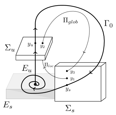
Figure 4 gives an impression of the homoclinic connection to a 3DL-saddle in the four-dimensional system. As we are interested in understanding the bifurcations close to the saddle and the homoclinic orbit, we define two Poincaré cross-sections,

ΣssubscriptΣ𝑠\displaystyle\Sigma_{s} ={(x1,x2,x3,x4)|x2=0},absentconditional-setsubscript𝑥1subscript𝑥2subscript𝑥3subscript𝑥4subscript𝑥20\displaystyle=\left\{(x_{1},x_{2},x_{3},x_{4})|x_{2}=0\right\}, (5)
ΣusubscriptΣ𝑢\displaystyle\Sigma_{u} ={(x1,x2,x3,x4)|x4=1},absentconditional-setsubscript𝑥1subscript𝑥2subscript𝑥3subscript𝑥4subscript𝑥41\displaystyle=\left\{(x_{1},x_{2},x_{3},x_{4})|x_{4}=1\right\}, (6)

and assume, after linearly rescaling variables if necessary, that the homoclinic orbit passes through these cross-sections at ys=(1,0,1,0)subscript𝑦𝑠1010y_{s}=(1,0,1,0) and yu=(0,0,0,1)subscript𝑦𝑢0001y_{u}=(0,0,0,1) respectively, for all parameter values along the primary homoclinic curve.
Refer to caption
Figure 4: The geometric construction of cross-sections close to the critical 3DL-saddle at (0,0,0,0)0000(0,0,0,0) and the homoclinic connection Γ0subscriptΓ0\Gamma_{0}, in order to obtain the map Π:ΣsΣs:Πmaps-tosubscriptΣ𝑠subscriptΣ𝑠\Pi:\Sigma_{s}\mapsto\Sigma_{s}. Here ΣusubscriptΣ𝑢\Sigma_{u} is defined by the cross-section x4=1subscript𝑥41x_{4}=1 and ΣssubscriptΣ𝑠\Sigma_{s} is the cross-section x3=0subscript𝑥30x_{3}=0. The homoclinic connection is assumed to pass through the points ys=(1,0,1,0)subscript𝑦𝑠1010y_{s}=(1,0,1,0) and yu=(0,0,0,1)subscript𝑦𝑢0001y_{u}=(0,0,0,1). The stable and unstable eigenspaces are Essubscript𝐸𝑠E_{s} and Eusubscript𝐸𝑢E_{u}, respectively.

Clearly, both cross-sections are transversal to the flow and to the stable and unstable eigenspaces. Thus, by following orbits starting from ΣssubscriptΣ𝑠\Sigma_{s} to ΣusubscriptΣ𝑢\Sigma_{u} and returning back to ΣssubscriptΣ𝑠\Sigma_{s}, we will be able to define a three-dimensional map ΠΠ\Pi mapping (a subset of) ΣssubscriptΣ𝑠\Sigma_{s} to itself. This map can then be used to study both periodic orbits and secondary homoclinic orbits.

We shall construct the map ΠΠ\Pi by composing two maps, Πloc:ΣsΣu:subscriptΠ𝑙𝑜𝑐maps-tosubscriptΣ𝑠subscriptΣ𝑢\Pi_{loc}:\Sigma_{s}\mapsto\Sigma_{u} and Πglob:ΣuΣs:subscriptΠ𝑔𝑙𝑜𝑏maps-tosubscriptΣ𝑢subscriptΣ𝑠\Pi_{glob}:\Sigma_{u}\mapsto\Sigma_{s}, i.e.

Π=ΠglobΠloc.ΠsubscriptΠ𝑔𝑙𝑜𝑏subscriptΠ𝑙𝑜𝑐\displaystyle\Pi=\Pi_{glob}\circ\Pi_{loc}. (7)

2.4 Derivation of the return map

We begin by computing the orbit of (4) starting from an arbitrary point in ΣssubscriptΣ𝑠\Sigma_{s}, close to yssubscript𝑦𝑠y_{s}. This will be used to define the map ΠlocsubscriptΠ𝑙𝑜𝑐\Pi_{loc}. The local map ΠlocsubscriptΠ𝑙𝑜𝑐\Pi_{loc} is the mapping from y1=(x1s,0,x3s,x4s)Σssubscript𝑦1superscriptsubscript𝑥1𝑠0superscriptsubscript𝑥3𝑠superscriptsubscript𝑥4𝑠subscriptΣ𝑠y_{1}=(x_{1}^{s},0,x_{3}^{s},x_{4}^{s})\in\Sigma_{s} to a point y2=(x1u,x2u,x3u,1)Σusubscript𝑦2superscriptsubscript𝑥1𝑢superscriptsubscript𝑥2𝑢superscriptsubscript𝑥3𝑢1subscriptΣ𝑢y_{2}=(x_{1}^{u},x_{2}^{u},x_{3}^{u},1)\in\Sigma_{u} close to yusubscript𝑦𝑢y_{u}, and is given by

Πloc:(x1sx3sx4s)(x1s(x4s)ν(μ)cos(1β(μ)lnx4s)x1s(x4s)ν(μ)sin(1β(μ)lnx4s)x3s(x4s)ν(μ)+μ1/β(μ)).:subscriptΠ𝑙𝑜𝑐maps-tosuperscriptsubscript𝑥1𝑠superscriptsubscript𝑥3𝑠superscriptsubscript𝑥4𝑠superscriptsubscript𝑥1𝑠superscriptsuperscriptsubscript𝑥4𝑠𝜈𝜇1𝛽𝜇superscriptsubscript𝑥4𝑠superscriptsubscript𝑥1𝑠superscriptsuperscriptsubscript𝑥4𝑠𝜈𝜇1𝛽𝜇superscriptsubscript𝑥4𝑠superscriptsubscript𝑥3𝑠superscriptsuperscriptsubscript𝑥4𝑠𝜈𝜇subscript𝜇1𝛽𝜇\Pi_{loc}:\left(\begin{array}[]{l}x_{1}^{s}\\ x_{3}^{s}\\ x_{4}^{s}\end{array}\right)\mapsto\left(\begin{array}[]{l}x_{1}^{s}(x_{4}^{s})^{\nu(\mu)}\cos\left(-\frac{1}{\beta(\mu)}\ln{x_{4}^{s}}\right)\\ x_{1}^{s}(x_{4}^{s})^{\nu(\mu)}\sin\left(-\frac{1}{\beta(\mu)}\ln{x_{4}^{s}}\right)\\ x_{3}^{s}(x_{4}^{s})^{\nu(\mu)+\mu_{1}/\beta(\mu)}\end{array}\right). (8)

where ν(μ)=γ(μ)/β(μ)𝜈𝜇𝛾𝜇𝛽𝜇\nu(\mu)=-\gamma(\mu)/\beta(\mu). Let γ0:=γ(0)assignsubscript𝛾0𝛾0\gamma_{0}:=\gamma(0) and β0:=β(0)assignsubscript𝛽0𝛽0\beta_{0}:=\beta(0). The quantity

ν0=γ0β0=δ0ϵ0subscript𝜈0subscript𝛾0subscript𝛽0subscript𝛿0subscriptitalic-ϵ0\nu_{0}=-\frac{\gamma_{0}}{\beta_{0}}=-\frac{\delta_{0}}{\epsilon_{0}} (9)

is called the saddle index. Note that the saddle quantity σ0subscript𝜎0\sigma_{0} is related to the saddle index (9) as follows:

ν0<1σ0>0,subscript𝜈01subscript𝜎00\displaystyle\nu_{0}<1\Longleftrightarrow\sigma_{0}>0,
ν0>1σ0<0.subscript𝜈01subscript𝜎00\displaystyle\nu_{0}>1\Longleftrightarrow\sigma_{0}<0.

We assume from now on that ν0<1subscript𝜈01\nu_{0}<1, so that only the wild case σ0>0subscript𝜎00\sigma_{0}>0 is considered.

For the global return map Πglob:ΣuΣs:subscriptΠ𝑔𝑙𝑜𝑏maps-tosubscriptΣ𝑢subscriptΣ𝑠\Pi_{glob}:\Sigma_{u}\mapsto\Sigma_{s}, we obviously cannot use (4). Instead we use a general C1superscript𝐶1C^{1} approximation of the flow from (0,0,0,1)0001(0,0,0,1) to (1,0,1,μ2)101subscript𝜇2(1,0,1,\mu_{2}). Here μ2subscript𝜇2\mu_{2} is the aforementioned splitting parameter. It controls the return of the orbit to the critical saddle. For μ2=0subscript𝜇20\mu_{2}=0 only, we have a primary homoclinic connection.

Thus, the following representation of ΠglobsubscriptΠ𝑔𝑙𝑜𝑏\Pi_{glob} can be used

Πglob:(x1ux2ux3u)(11μ2)+(a11(μ)a12(μ)a13(μ)a21(μ)a22(μ)a23(μ)a31(μ)a32(μ)a33(μ))(x1ux2ux3u)+o(xu),:subscriptΠ𝑔𝑙𝑜𝑏maps-tosuperscriptsubscript𝑥1𝑢superscriptsubscript𝑥2𝑢superscriptsubscript𝑥3𝑢11subscript𝜇2subscript𝑎11𝜇subscript𝑎12𝜇subscript𝑎13𝜇subscript𝑎21𝜇subscript𝑎22𝜇subscript𝑎23𝜇subscript𝑎31𝜇subscript𝑎32𝜇subscript𝑎33𝜇superscriptsubscript𝑥1𝑢superscriptsubscript𝑥2𝑢superscriptsubscript𝑥3𝑢𝑜normsuperscript𝑥𝑢\Pi_{glob}:\left(\begin{array}[]{l}x_{1}^{u}\\ x_{2}^{u}\\ x_{3}^{u}\end{array}\right)\mapsto\left(\begin{array}[]{l}1\\ 1\\ \mu_{2}\end{array}\right)+\left(\begin{array}[]{lll}a_{11}(\mu)&a_{12}(\mu)&a_{13}(\mu)\\ a_{21}(\mu)&a_{22}(\mu)&a_{23}(\mu)\\ a_{31}(\mu)&a_{32}(\mu)&a_{33}(\mu)\end{array}\right)\left(\begin{array}[]{l}x_{1}^{u}\\ x_{2}^{u}\\ x_{3}^{u}\end{array}\right)+o(\|x^{u}\|), (10)

where xu=(x1u,x2u,x3u)superscript𝑥𝑢superscriptsubscript𝑥1𝑢superscriptsubscript𝑥2𝑢superscriptsubscript𝑥3𝑢x^{u}=(x_{1}^{u},x_{2}^{u},x_{3}^{u}). For A0=[aij(0)]subscript𝐴0delimited-[]subscript𝑎𝑖𝑗0A_{0}=[a_{ij}(0)] we also have det(A0)0subscript𝐴00\det(A_{0})\neq 0 which follows from the invertibility of ΠglobsubscriptΠ𝑔𝑙𝑜𝑏\Pi_{glob} for μ𝜇\mu small enough.

Now, (8) and (10) together give us the full return map Π=ΠglobΠlocΠsubscriptΠ𝑔𝑙𝑜𝑏subscriptΠ𝑙𝑜𝑐\Pi=\Pi_{glob}\circ\Pi_{loc}. Keeping the dependence of all coefficients on μ𝜇\mu implicit, we can write ΠΠ\Pi as

Π:(x1sx3sx4s)(1+b1x1s(x4s)νcos(1βlnx4s+θ1)+b2x3s(x4s)ν+μ1/β1+b3x1s(x4s)νsin(1βlnx4s+θ2)+b4x3s(x4s)ν+μ1/βμ2+b5x1s(x4s)νsin(1βlnx4s+θ3)+b6x3s(x4s)ν+μ1/β)+o(xsν),:Πmaps-tosuperscriptsubscript𝑥1𝑠superscriptsubscript𝑥3𝑠superscriptsubscript𝑥4𝑠1subscript𝑏1superscriptsubscript𝑥1𝑠superscriptsuperscriptsubscript𝑥4𝑠𝜈1𝛽superscriptsubscript𝑥4𝑠subscript𝜃1subscript𝑏2superscriptsubscript𝑥3𝑠superscriptsuperscriptsubscript𝑥4𝑠𝜈subscript𝜇1𝛽1subscript𝑏3superscriptsubscript𝑥1𝑠superscriptsuperscriptsubscript𝑥4𝑠𝜈1𝛽superscriptsubscript𝑥4𝑠subscript𝜃2subscript𝑏4superscriptsubscript𝑥3𝑠superscriptsuperscriptsubscript𝑥4𝑠𝜈subscript𝜇1𝛽subscript𝜇2subscript𝑏5superscriptsubscript𝑥1𝑠superscriptsuperscriptsubscript𝑥4𝑠𝜈1𝛽superscriptsubscript𝑥4𝑠subscript𝜃3subscript𝑏6superscriptsubscript𝑥3𝑠superscriptsuperscriptsubscript𝑥4𝑠𝜈subscript𝜇1𝛽𝑜superscriptnormsuperscript𝑥𝑠𝜈\Pi:\left(\begin{array}[]{l}x_{1}^{s}\\ x_{3}^{s}\\ x_{4}^{s}\end{array}\right)\mapsto\left(\begin{array}[]{l}1+b_{1}x_{1}^{s}(x_{4}^{s})^{\nu}\cos\left(-\frac{1}{\beta}\ln x_{4}^{s}+\theta_{1}\right)+b_{2}x_{3}^{s}(x_{4}^{s})^{\nu+\mu_{1}/\beta}\\ 1+b_{3}x_{1}^{s}(x_{4}^{s})^{\nu}\sin\left(-\frac{1}{\beta}\ln x_{4}^{s}+\theta_{2}\right)+b_{4}x_{3}^{s}(x_{4}^{s})^{\nu+\mu_{1}/\beta}\\ \mu_{2}+b_{5}x_{1}^{s}(x_{4}^{s})^{\nu}\sin\left(-\frac{1}{\beta}\ln x_{4}^{s}+\theta_{3}\right)+b_{6}x_{3}^{s}(x_{4}^{s})^{\nu+\mu_{1}/\beta}\end{array}\right)+o(\|x^{s}\|^{\nu}), (11)

where xs=(x1s,x3s,x4s)superscript𝑥𝑠superscriptsubscript𝑥1𝑠superscriptsubscript𝑥3𝑠superscriptsubscript𝑥4𝑠x^{s}=(x_{1}^{s},x_{3}^{s},x_{4}^{s}) and

sinθ1=a12a112+a122,cosθ2=a22a212+a222,cosθ3=a32a312+a322,b1=a112+a122,b3=a212+a222,b5=a312+a322,b2=a13,b4=a23,and b6=a33.subscript𝜃1subscript𝑎12superscriptsubscript𝑎112superscriptsubscript𝑎122subscript𝜃2subscript𝑎22superscriptsubscript𝑎212superscriptsubscript𝑎222subscript𝜃3subscript𝑎32superscriptsubscript𝑎312superscriptsubscript𝑎322subscript𝑏1superscriptsubscript𝑎112superscriptsubscript𝑎122subscript𝑏3superscriptsubscript𝑎212superscriptsubscript𝑎222subscript𝑏5superscriptsubscript𝑎312superscriptsubscript𝑎322subscript𝑏2subscript𝑎13subscript𝑏4subscript𝑎23and subscript𝑏6subscript𝑎33\begin{array}[]{lll}\sin\theta_{1}=-\frac{a_{12}}{\sqrt{a_{11}^{2}+a_{12}^{2}}},&\cos\theta_{2}=\frac{a_{22}}{\sqrt{a_{21}^{2}+a_{22}^{2}}},&\cos\theta_{3}=\frac{a_{32}}{\sqrt{a_{31}^{2}+a_{32}^{2}}},\\ b_{1}=\sqrt{a_{11}^{2}+a_{12}^{2}},&b_{3}=\sqrt{a_{21}^{2}+a_{22}^{2}},&b_{5}=\sqrt{a_{31}^{2}+a_{32}^{2}},\\ b_{2}=a_{13},&b_{4}=a_{23},&\textnormal{and }\ b_{6}=a_{33}.\end{array} (12)

Following LABEL:Gonchenko1997, we make the smooth invertible transformation x4sx4sexp(θ3β)maps-tosuperscriptsubscript𝑥4𝑠superscriptsubscript𝑥4𝑠subscript𝜃3𝛽x_{4}^{s}\mapsto x_{4}^{s}\exp\left(\theta_{3}\beta\right) to eliminate θ3subscript𝜃3\theta_{3}. This gives

Π:(x1x3x4)(1+α1x1x4νcos(1βlnx4+ϕ1)+α2x3x4ν+μ1/β1+α3x1x4νsin(1βlnx4+ϕ2)+α4x3x4ν+μ1/βμ2+C1x1x4νsin(1βlnx4)+C2x3x4ν+μ1/β)+o(xν),:Πmaps-tosubscript𝑥1subscript𝑥3subscript𝑥41subscript𝛼1subscript𝑥1superscriptsubscript𝑥4𝜈1𝛽subscript𝑥4subscriptitalic-ϕ1subscript𝛼2subscript𝑥3superscriptsubscript𝑥4𝜈subscript𝜇1𝛽1subscript𝛼3subscript𝑥1superscriptsubscript𝑥4𝜈1𝛽subscript𝑥4subscriptitalic-ϕ2subscript𝛼4subscript𝑥3superscriptsubscript𝑥4𝜈subscript𝜇1𝛽subscript𝜇2subscript𝐶1subscript𝑥1superscriptsubscript𝑥4𝜈1𝛽subscript𝑥4subscript𝐶2subscript𝑥3superscriptsubscript𝑥4𝜈subscript𝜇1𝛽𝑜superscriptnorm𝑥𝜈\Pi:\left(\begin{array}[]{l}x_{1}\\ x_{3}\\ x_{4}\end{array}\right)\mapsto\left(\begin{array}[]{l}1+\alpha_{1}x_{1}x_{4}^{\nu}\cos\left(-\frac{1}{\beta}\ln x_{4}+\phi_{1}\right)+\alpha_{2}x_{3}x_{4}^{\nu+\mu_{1}/\beta}\\ 1+\alpha_{3}x_{1}x_{4}^{\nu}\sin\left(-\frac{1}{\beta}\ln x_{4}+\phi_{2}\right)+\alpha_{4}x_{3}x_{4}^{\nu+\mu_{1}/\beta}\\ \mu_{2}+C_{1}x_{1}x_{4}^{\nu}\sin\left(-\frac{1}{\beta}\ln x_{4}\right)+C_{2}x_{3}x_{4}^{\nu+\mu_{1}/\beta}\end{array}\right)+o(\|x\|^{\nu}), (13)

where we have dropped the superscript ‘s𝑠s’ from the coordinates of x=(x1,x3,x4)𝑥subscript𝑥1subscript𝑥3subscript𝑥4x=(x_{1},x_{3},x_{4}) for convenience, and where

ϕ1=θ1θ3,ϕ2=θ2θ3,α1=b1exp(θ3βν),α2=b2exp((ν+μ1/β)θ3β),α3=b3exp(θ3βν),α4=b4exp((ν+μ1/β)θ3β),C1=b5exp(θ3βν)and C2=b2exp((ν+μ1/β)θ3β).subscriptitalic-ϕ1subscript𝜃1subscript𝜃3subscriptitalic-ϕ2subscript𝜃2subscript𝜃3subscript𝛼1subscript𝑏1subscript𝜃3𝛽𝜈subscript𝛼2subscript𝑏2𝜈subscript𝜇1𝛽subscript𝜃3𝛽subscript𝛼3subscript𝑏3subscript𝜃3𝛽𝜈subscript𝛼4subscript𝑏4𝜈subscript𝜇1𝛽subscript𝜃3𝛽subscript𝐶1subscript𝑏5subscript𝜃3𝛽𝜈and subscript𝐶2subscript𝑏2𝜈subscript𝜇1𝛽subscript𝜃3𝛽\displaystyle\begin{array}[]{ll}\phi_{1}=\theta_{1}-\theta_{3},&\phi_{2}=\theta_{2}-\theta_{3},\\ \alpha_{1}=b_{1}\exp(\theta_{3}\beta\nu),&\alpha_{2}=b_{2}\exp((\nu+\mu_{1}/\beta)\theta_{3}\beta),\\ \alpha_{3}=b_{3}\exp(\theta_{3}\beta\nu),&\alpha_{4}=b_{4}\exp((\nu+\mu_{1}/\beta)\theta_{3}\beta),\\ C_{1}=b_{5}\exp(\theta_{3}\beta\nu)&\textnormal{and }\ C_{2}=b_{2}\exp((\nu+\mu_{1}/\beta)\theta_{3}\beta).\end{array} (18)

Observe that all constants αjsubscript𝛼𝑗\alpha_{j} and Cksubscript𝐶𝑘C_{k} depend on μ𝜇\mu and that C1>0subscript𝐶10C_{1}>0. Let us denote by αj0superscriptsubscript𝛼𝑗0\alpha_{j}^{0} and Cj0superscriptsubscript𝐶𝑗0C_{j}^{0} their critical values at μ=0𝜇0\mu=0.

Truncating the o(xν)𝑜superscriptnorm𝑥𝜈o(\|x\|^{\nu})-terms in (13) and taking only the critical values of all constants, we define

G(x,μ):=(1+α10x1x4ν0cos(1β0lnx4+ϕ10)+α20x3x4ν0+μ1/β01+α30x1x4ν0sin(1β0lnx4+ϕ20)+α40x3x4ν0+μ1/β0μ2+C10x1x4ν0sin(1β0lnx4)+C20x3x4ν0+μ1/β0).assign𝐺𝑥𝜇1subscriptsuperscript𝛼01subscript𝑥1superscriptsubscript𝑥4subscript𝜈01subscript𝛽0subscript𝑥4subscriptsuperscriptitalic-ϕ01subscriptsuperscript𝛼02subscript𝑥3superscriptsubscript𝑥4subscript𝜈0subscript𝜇1subscript𝛽01subscriptsuperscript𝛼03subscript𝑥1superscriptsubscript𝑥4subscript𝜈01subscript𝛽0subscript𝑥4subscriptsuperscriptitalic-ϕ02subscriptsuperscript𝛼04subscript𝑥3superscriptsubscript𝑥4subscript𝜈0subscript𝜇1subscript𝛽0subscript𝜇2subscriptsuperscript𝐶01subscript𝑥1superscriptsubscript𝑥4subscript𝜈01subscript𝛽0subscript𝑥4subscriptsuperscript𝐶02subscript𝑥3superscriptsubscript𝑥4subscript𝜈0subscript𝜇1subscript𝛽0G(x,\mu):=\left(\begin{array}[]{l}1+\alpha^{0}_{1}x_{1}x_{4}^{\nu_{0}}\cos\left(-\frac{1}{\beta_{0}}\ln x_{4}+\phi^{0}_{1}\right)+\alpha^{0}_{2}x_{3}x_{4}^{\nu_{0}+\mu_{1}/{\beta_{0}}}\\ 1+\alpha^{0}_{3}x_{1}x_{4}^{\nu_{0}}\sin\left(-\frac{1}{\beta_{0}}\ln x_{4}+\phi^{0}_{2}\right)+\alpha^{0}_{4}x_{3}x_{4}^{\nu_{0}+\mu_{1}/{\beta_{0}}}\\ \mu_{2}+C^{0}_{1}x_{1}x_{4}^{\nu_{0}}\sin\left(-\frac{1}{\beta_{0}}\ln x_{4}\right)+C^{0}_{2}x_{3}x_{4}^{\nu_{0}+\mu_{1}/{\beta_{0}}}\end{array}\right). (19)

This map G𝐺G is the final form of the 3D model return map that we will use for the numerical analysis ahead.

Now, to analyze periodic orbits close to the homoclinic connection with respect to the critical 3DL-saddle, we look for fixed points of the map ΠΠ\Pi given by (13). These fixed points correspond to periodic orbits in the original ODE system. Bifurcations of these fixed points describe the various local bifurcations of the corresponding periodic orbits.

The fixed point condition for map (13) is

(x1x3x4)=(1+α1x1x4νcos(1βlnx4+ϕ1)+α2x3x4ν+μ1/β1+α3x1x4νsin(1βlnx4+ϕ2)+α4x3x4ν+μ1/βμ2+C1x1x4νsin(1βlnx4)+C2x3x4ν+μ1/β)+o(xν),subscript𝑥1subscript𝑥3subscript𝑥41subscript𝛼1subscript𝑥1superscriptsubscript𝑥4𝜈1𝛽subscript𝑥4subscriptitalic-ϕ1subscript𝛼2subscript𝑥3superscriptsubscript𝑥4𝜈subscript𝜇1𝛽1subscript𝛼3subscript𝑥1superscriptsubscript𝑥4𝜈1𝛽subscript𝑥4subscriptitalic-ϕ2subscript𝛼4subscript𝑥3superscriptsubscript𝑥4𝜈subscript𝜇1𝛽subscript𝜇2subscript𝐶1subscript𝑥1superscriptsubscript𝑥4𝜈1𝛽subscript𝑥4subscript𝐶2subscript𝑥3superscriptsubscript𝑥4𝜈subscript𝜇1𝛽𝑜superscriptnorm𝑥𝜈\left(\begin{array}[]{l}x_{1}\\ x_{3}\\ x_{4}\end{array}\right)=\left(\begin{array}[]{l}1+\alpha_{1}x_{1}x_{4}^{\nu}\cos\left(-\frac{1}{\beta}\ln x_{4}+\phi_{1}\right)+\alpha_{2}x_{3}x_{4}^{\nu+\mu_{1}/{\beta}}\\ 1+\alpha_{3}x_{1}x_{4}^{\nu}\sin\left(-\frac{1}{\beta}\ln x_{4}+\phi_{2}\right)+\alpha_{4}x_{3}x_{4}^{\nu+\mu_{1}/{\beta}}\\ \mu_{2}+C_{1}x_{1}x_{4}^{\nu}\sin\left(-\frac{1}{\beta}\ln x_{4}\right)+C_{2}x_{3}x_{4}^{\nu+\mu_{1}/{\beta}}\end{array}\right)+o(\|x\|^{\nu}), (20)

where all constants αjsubscript𝛼𝑗\alpha_{j} and Cksubscript𝐶𝑘C_{k} still depend on μ𝜇\mu. For non-degeneracy, we require that real constants C1subscript𝐶1C_{1} and C2subscript𝐶2C_{2} are nonzero. We justify this later. Substituting the expressions for x1subscript𝑥1x_{1} and x3subscript𝑥3x_{3} from (20) in the expression for x4subscript𝑥4x_{4}, we get

x4=μ2+C1x4νsin(1βlnx4)+C2x4ν+μ1/β+o(|x4|ν),subscript𝑥4subscript𝜇2subscript𝐶1superscriptsubscript𝑥4𝜈1𝛽subscript𝑥4subscript𝐶2superscriptsubscript𝑥4𝜈subscript𝜇1𝛽𝑜superscriptsubscript𝑥4𝜈\displaystyle x_{4}=\mu_{2}+C_{1}x_{4}^{\nu}\sin\left(-\frac{1}{\beta}\ln x_{4}\right)+C_{2}x_{4}^{\nu+\mu_{1}/\beta}+o(|x_{4}|^{\nu}), (21)

as our one-dimensional fixed point condition. As we are interested behavior close to (1,0,1,0)1010(1,0,1,0) on the cross-section ΣssubscriptΣ𝑠\Sigma_{s}, we consider only the leading terms of (21) and introduce the following scalar model map:

F(x,μ):=μ2+C10xν0sin(1β0lnx)+C20xν0+μ1/β0.assign𝐹𝑥𝜇subscript𝜇2subscriptsuperscript𝐶01superscript𝑥subscript𝜈01subscript𝛽0𝑥subscriptsuperscript𝐶02superscript𝑥subscript𝜈0subscript𝜇1subscript𝛽0\displaystyle F(x,\mu):=\mu_{2}+C^{0}_{1}x^{\nu_{0}}\sin\left(-\frac{1}{\beta_{0}}\ln x\right)+C^{0}_{2}x^{\nu_{0}+\mu_{1}/{\beta_{0}}}. (22)

The extra additive term C20xν0+μ1/β0subscriptsuperscript𝐶02superscript𝑥subscript𝜈0subscript𝜇1subscript𝛽0C^{0}_{2}x^{\nu_{0}+\mu_{1}/{\beta_{0}}} is what makes this map different from the scalar model maps describing the codim 1 saddle-focus case.

If we were to set C10subscriptsuperscript𝐶01C^{0}_{1} to zero, then we would obtain finitely many fixed points for all values of ν0,μ1,β0,μ2subscript𝜈0subscript𝜇1subscript𝛽0subscript𝜇2\nu_{0},\mu_{1},\beta_{0},\mu_{2} and C20subscriptsuperscript𝐶02C^{0}_{2}. If we set C20subscriptsuperscript𝐶02C^{0}_{2} to zero, we get the codim 1 saddle-focus case. Thus we assume

  1. (A.5) C10C200.subscriptsuperscript𝐶01subscriptsuperscript𝐶020C^{0}_{1}C^{0}_{2}\neq 0.

3 Analysis of the scalar model map

In this section, we study bifurcations of fixed points of the map (23). To stay close to the 3DL bifurcation, we only work with small values of x𝑥x and μ𝜇\mu. To simplify notations, we rewrite the scalar model map as

F(x,μ):=μ2+C1xνsin(1βlnx)+C2xν+μ1/β,assign𝐹𝑥𝜇subscript𝜇2subscript𝐶1superscript𝑥𝜈1𝛽𝑥subscript𝐶2superscript𝑥𝜈subscript𝜇1𝛽\displaystyle F(x,\mu):=\mu_{2}+C_{1}x^{\nu}\sin\left(-\frac{1}{\beta}\ln x\right)+C_{2}x^{\nu+\mu_{1}/{\beta}}, (23)

assuming that ν,β𝜈𝛽\nu,\beta, and C1,2subscript𝐶12C_{1,2} are fixed at their critical values.
Refer to caption
Refer to caption
Refer to caption
Refer to caption
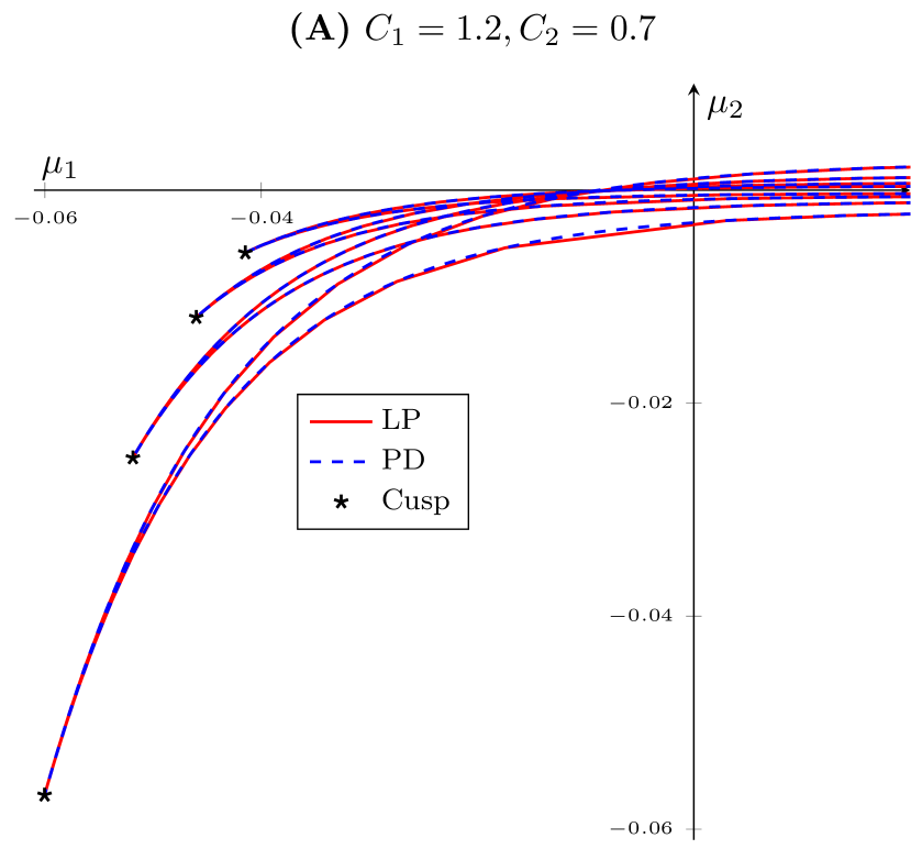
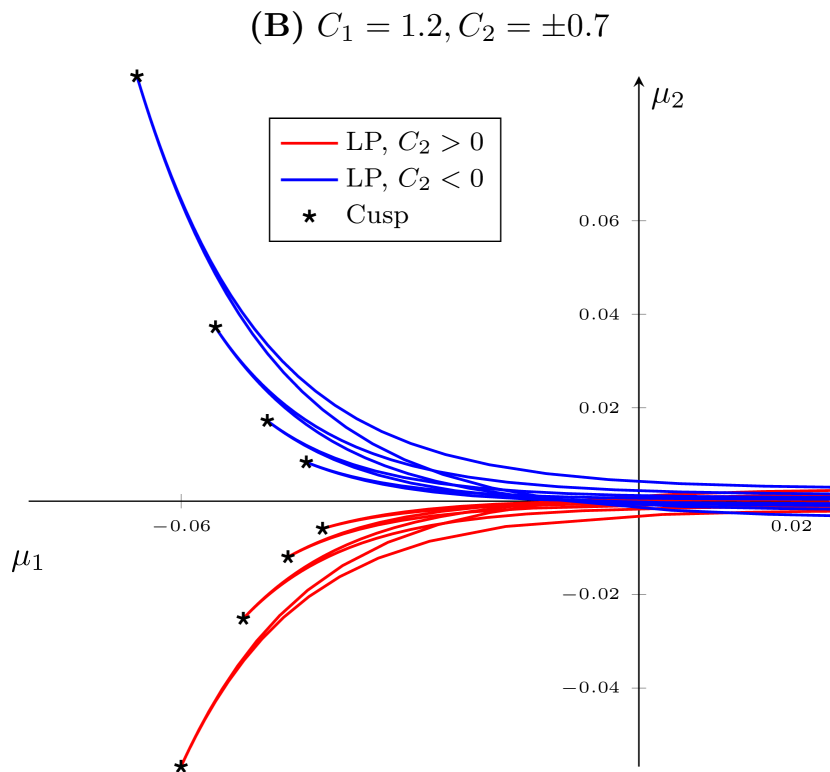
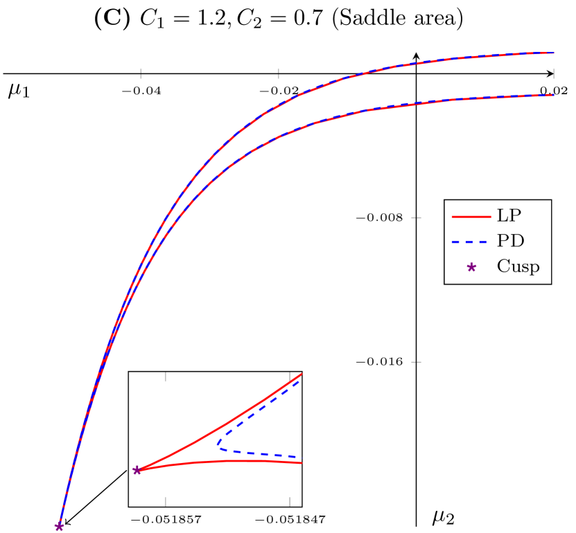
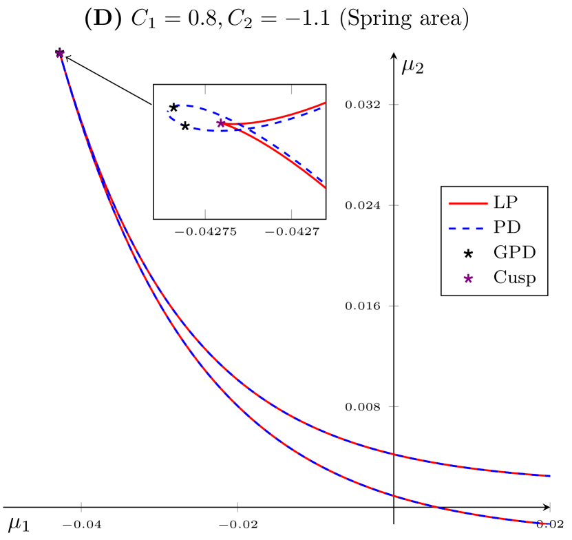
Figure 5: Primary LP and PD bifurcation curves obtained by numerical continuation, for the map (23) for some representative values of C1subscript𝐶1C_{1} and C2subscript𝐶2C_{2}. In panel (A) we plot 4 pairs of these curves. All of them have the same global structure. There are two types of codimension 2 points that can be found along these curves: Cusp (on LP curves) and GPD (along PD curves). In panel (B) we see what happens when we switch the sign of C2subscript𝐶2C_{2}, the horns move from μ2>0subscript𝜇20\mu_{2}>0 to μ2<0subscript𝜇20\mu_{2}<0. In panel (C) and (D) we see examples of one PD and LP curve with the saddle area and spring area respectively (zoomed in). In the insets, μ2subscript𝜇2\mu_{2} is scaled for convenience.

3.1 Numerical continuation results

Using the continuation package MatcontM [19, 20], we obtained many LP and PD bifurcation curves, which form interesting structures. There is strong evidence that there exist infinitely many PD and LP curves in the (μ1,μ2)subscript𝜇1subscript𝜇2(\mu_{1},\mu_{2})-parameter space. Several such curves can be seen in Figure 5. We make the following observations:

  1. 1.

    The curves exhibit a repetitive behavior: two branches of one LP curve meet to form a horn. Apparently, infinitely many such ‘horns’ exist. The sequence of these ‘horns’ in the parameter space appears to approach μ2=0subscript𝜇20\mu_{2}=0 asymptotically, which is the curve of primary homoclinic orbits. Also, the tips of the ‘horns’ are always located entirely in either the second, or third quadrant of the (μ1,μ2)subscript𝜇1subscript𝜇2(\mu_{1},\mu_{2})-space.

  2. 2.

    The PD and LP curves appear to coincide on visual inspection, and there can exist GPD points in the vicinity of the tip of the LP horn.

  3. 3.

    The tip each LP ‘horn’ is a cusp point. These cusps always exist, for all values of C1subscript𝐶1C_{1} and C2subscript𝐶2C_{2} and form a sequence that appears to approach the origin μ=0𝜇0\mu=0.

  4. 4.

    Upon closer inspection, we observe that there exists either of the two subtle structures near the top of every LP ‘horn’. One is a spring area, where the PD curve loops around the cusp point. The other is a saddle area, where the PD curve makes a sharp turn close to the cusp, see the insets in Figure 5. The spring area is accompanied by two GPD points along the PD loop. These points are absent in a saddle area. Mira et al. [17] discuss in detail the spring and saddle areas, including transitions from one case to the other and their genericity.

  5. 5.

    The global behavior of this set of curves depends on parameters C1subscript𝐶1C_{1} and C2subscript𝐶2C_{2}. For example, by switching the sign of C2subscript𝐶2C_{2}, the set of curves can be moved from the second to the third quadrant of the μ𝜇\mu-space, or vice-versa. The presence of saddle or spring areas depend on the parameters C1subscript𝐶1C_{1} and C2subscript𝐶2C_{2} but the exact conditions are not clear.

In the sections ahead we support most of the observations by looking at analytical asymptotics of the LP and PD bifurcation curves of (23).
Refer to caption
Refer to caption
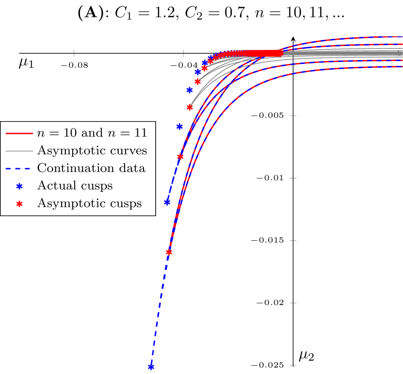
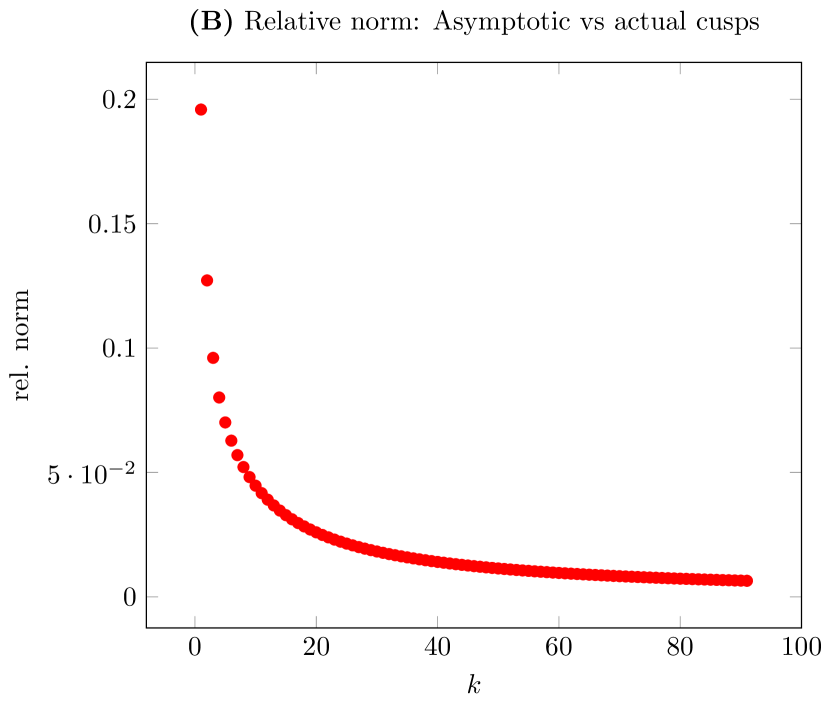
Figure 6: Plots of asymptotic curves and PD/LP curves (obtained from continuation). In (A) we see how successive asymptotic curves in n𝑛n approximate the set of PD/LP curves. Here, cusps are obtained by performing Newton iterations to the defining system of the cusp bifurcation with starting points as the asymptotic cusps. In (B), convergence of the asymptotic cusps to the actual cusps is observed. The corresponding values of n𝑛n in both plots are n=10,11,90𝑛101190n=10,11...,90.

3.2 Asymptotics

In this section we derive approximate solutions to the LP and PD conditions, and use them to justify numerical observations. As we are interested in solutions close to the 3DL bifurcation point (μ1,μ2)=(0,0)subscript𝜇1subscript𝜇200(\mu_{1},\mu_{2})=(0,0) we assume that x,μ1𝑥subscript𝜇1x,\mu_{1} and μ2subscript𝜇2\mu_{2} are sufficiently small. As we investigate only the wild case we restrict ourselves to ν<1𝜈1\nu<1.

3.2.1 LP horns and cusp points

For the scalar model map (23) the fixed point condition is given by

μ2+C1xνsin(1βlnx)+C2xν+μ1/βx=0.subscript𝜇2subscript𝐶1superscript𝑥𝜈1𝛽𝑥subscript𝐶2superscript𝑥𝜈subscript𝜇1𝛽𝑥0\mu_{2}+C_{1}x^{\nu}\sin\left(-\frac{1}{\beta}\ln x\right)+C_{2}x^{\nu+\mu_{1}/\beta}-x=0. (24)

We parametrize x𝑥x using the following relation,

1βlnx=2πn+θ,1𝛽𝑥2𝜋𝑛𝜃-\frac{1}{\beta}\ln x=2\pi n+\theta, (25)

for large n𝑛n\in\mathbb{N} and θ(0,2π)𝜃02𝜋\theta\in(0,2\pi). Thus, (24) becomes

μ2+C1eβν(2πn+θ)sinθ+C2eβ(ν+μ1/β)(2πn+θ)eβ(2πn+θ)=0.subscript𝜇2subscript𝐶1superscript𝑒𝛽𝜈2𝜋𝑛𝜃𝜃subscript𝐶2superscript𝑒𝛽𝜈subscript𝜇1𝛽2𝜋𝑛𝜃superscript𝑒𝛽2𝜋𝑛𝜃0\mu_{2}+C_{1}e^{-\beta\nu(2\pi n+\theta)}\sin\theta+C_{2}e^{-\beta(\nu+\mu_{1}/\beta)(2\pi n+\theta)}-e^{-\beta(2\pi n+\theta)}=0. (26)

Let us define

Φ(θ,μ1,μ2):=μ2+C1eβν(2πn+θ)sinθ+C2eβ(ν+μ1/β)(2πn+θ)eβ(2πn+θ).assignΦ𝜃subscript𝜇1subscript𝜇2subscript𝜇2subscript𝐶1superscript𝑒𝛽𝜈2𝜋𝑛𝜃𝜃subscript𝐶2superscript𝑒𝛽𝜈subscript𝜇1𝛽2𝜋𝑛𝜃superscript𝑒𝛽2𝜋𝑛𝜃\Phi(\theta,\mu_{1},\mu_{2}):=\mu_{2}+C_{1}e^{-\beta\nu(2\pi n+\theta)}\sin\theta+C_{2}e^{-\beta(\nu+\mu_{1}/\beta)(2\pi n+\theta)}-e^{-\beta(2\pi n+\theta)}. (27)

Then

Φθ(θ,μ1,μ2)=0,subscriptΦ𝜃𝜃subscript𝜇1subscript𝜇20\Phi_{\theta}(\theta,\mu_{1},\mu_{2})=0,

is the extra condition for an LP point. Computing the derivative, we get

C1(βνsinθcosθ)+C2(βν+μ1)eμ1(2πn+θ)βeβ(1ν)(2πn+θ)=0.subscript𝐶1𝛽𝜈𝜃𝜃subscript𝐶2𝛽𝜈subscript𝜇1superscript𝑒subscript𝜇12𝜋𝑛𝜃𝛽superscript𝑒𝛽1𝜈2𝜋𝑛𝜃0C_{1}\left(\beta\nu\sin\theta-\cos\theta\right)+C_{2}(\beta\nu+\mu_{1})e^{-\mu_{1}(2\pi n+\theta)}-\beta e^{-\beta(1-\nu)(2\pi n+\theta)}=0. (28)

We now simultaneously solve (24) and (28) to obtain a sequence of functions μ2(n)(μ1)superscriptsubscript𝜇2𝑛subscript𝜇1\mu_{2}^{(n)}(\mu_{1}) which describe the sequence of LP ‘horns’ already observed numerically. Thus, rewriting (28), we have

βνsinθcosθ=C2C1(βν+μ1)eμ1(2πn+θ)+βC1eβ(1ν)(2πn+θ)=C2C1(βν+μ1)e2πμ1n[1μ1θ+O(μ12)]+O(eαn)=C2C1e2πμ1n[βν(1βνθ)μ1+O(μ12)]+O(eαn),𝛽𝜈𝜃𝜃absentsubscript𝐶2subscript𝐶1𝛽𝜈subscript𝜇1superscript𝑒subscript𝜇12𝜋𝑛𝜃𝛽subscript𝐶1superscript𝑒𝛽1𝜈2𝜋𝑛𝜃missing-subexpressionabsentsubscript𝐶2subscript𝐶1𝛽𝜈subscript𝜇1superscript𝑒2𝜋subscript𝜇1𝑛delimited-[]1subscript𝜇1𝜃𝑂superscriptsubscript𝜇12𝑂superscript𝑒𝛼𝑛missing-subexpressionabsentsubscript𝐶2subscript𝐶1superscript𝑒2𝜋subscript𝜇1𝑛delimited-[]𝛽𝜈1𝛽𝜈𝜃subscript𝜇1𝑂superscriptsubscript𝜇12𝑂superscript𝑒𝛼𝑛\begin{array}[]{ll}\beta\nu\sin\theta-\cos\theta&=-\frac{C_{2}}{C_{1}}\left(\beta\nu+\mu_{1}\right)e^{-\mu_{1}(2\pi n+\theta)}+\frac{\beta}{C_{1}}e^{-\beta(1-\nu)(2\pi n+\theta)}\\ &=-\frac{C_{2}}{C_{1}}\left(\beta\nu+\mu_{1}\right)e^{-2\pi\mu_{1}n}\left[1-\mu_{1}\theta+O(\mu_{1}^{2})\right]+O(e^{-\alpha n})\\ &=-\frac{C_{2}}{C_{1}}e^{-2\pi\mu_{1}n}\left[\beta\nu-(1-\beta\nu\theta)\mu_{1}+O(\mu_{1}^{2})\right]+O(e^{-\alpha n}),\end{array} (29)

where α=2πβ(1ν)>0𝛼2𝜋𝛽1𝜈0\alpha=2\pi\beta(1-\nu)>0. Collecting trigonometric terms on the left we get

sin(θϕ)=11+β2ν2C2C1e2πμ1n[βν(1βνθ)μ1+O(μ12)]+O(eαn),𝜃italic-ϕ11superscript𝛽2superscript𝜈2subscript𝐶2subscript𝐶1superscript𝑒2𝜋subscript𝜇1𝑛delimited-[]𝛽𝜈1𝛽𝜈𝜃subscript𝜇1𝑂superscriptsubscript𝜇12𝑂superscript𝑒𝛼𝑛\sin(\theta-\phi)=-\frac{1}{\sqrt{1+\beta^{2}\nu^{2}}}\frac{C_{2}}{C_{1}}e^{-2\pi\mu_{1}n}\left[\beta\nu-(1-\beta\nu\theta)\mu_{1}+O(\mu_{1}^{2})\right]+O(e^{-\alpha n}), (30)

where sinϕ=(1+β2ν2)1/2italic-ϕsuperscript1superscript𝛽2superscript𝜈212\sin\phi=(1+\beta^{2}\nu^{2})^{-1/2} and ϕ(0,π/2)italic-ϕ0𝜋2\phi\in(0,\pi/2). Note that for large n𝑛n and negative μ1subscript𝜇1\mu_{1}, the corresponding solution θ𝜃\theta exists only for small |μ1|subscript𝜇1|\mu_{1}|. Let

θ0n:=arcsin(βν1+β2ν2C2C1e2πμ1n).assignsubscriptsuperscript𝜃𝑛0𝛽𝜈1superscript𝛽2superscript𝜈2subscript𝐶2subscript𝐶1superscript𝑒2𝜋subscript𝜇1𝑛\theta^{n}_{0}:=\arcsin\left(-\frac{\beta\nu}{\sqrt{1+\beta^{2}\nu^{2}}}\frac{C_{2}}{C_{1}}e^{-2\pi\mu_{1}n}\right). (31)

Then we have two solutions,

θ1=ϕ+θ0n+δi1(2π)+O(μ1),θ2=ϕ+πθ0n+O(μ1),subscript𝜃1italic-ϕsubscriptsuperscript𝜃𝑛0subscript𝛿𝑖12𝜋𝑂subscript𝜇1subscript𝜃2italic-ϕ𝜋subscriptsuperscript𝜃𝑛0𝑂subscript𝜇1\begin{array}[]{l}\theta_{1}=\phi+\theta^{n}_{0}+\delta_{i1}(2\pi)+O(\mu_{1}),\\ \theta_{2}=\phi+\pi-\theta^{n}_{0}+O(\mu_{1}),\end{array} (32)

where i=sign(C2)𝑖signsubscript𝐶2i=-\textnormal{sign}(C_{2}) and δijsubscript𝛿𝑖𝑗\delta_{ij} is the Kronecker delta.

For each n𝑛n we obtain two solutions θ𝜃\theta given by (32). The corresponding functions μ2(n)(μ1)superscriptsubscript𝜇2𝑛subscript𝜇1\mu_{2}^{(n)}(\mu_{1}) are obtained from the first equation of (26),

{μ2(n,1)(μ1)=C1eβν(2πn+θ1)sinθ1C2eβ(ν+μ1/β)(2πn+θ1)+eβ(2πn+θ1),μ2(n,2)(μ1)=C1eβν(2πn+θ2)sinθ2C2eβ(ν+μ1/β)(2πn+θ2)+eβ(2πn+θ2).casessuperscriptsubscript𝜇2𝑛1subscript𝜇1subscript𝐶1superscript𝑒𝛽𝜈2𝜋𝑛subscript𝜃1subscript𝜃1subscript𝐶2superscript𝑒𝛽𝜈subscript𝜇1𝛽2𝜋𝑛subscript𝜃1superscript𝑒𝛽2𝜋𝑛subscript𝜃1superscriptsubscript𝜇2𝑛2subscript𝜇1subscript𝐶1superscript𝑒𝛽𝜈2𝜋𝑛subscript𝜃2subscript𝜃2subscript𝐶2superscript𝑒𝛽𝜈subscript𝜇1𝛽2𝜋𝑛subscript𝜃2superscript𝑒𝛽2𝜋𝑛subscript𝜃2\left\{\begin{array}[]{l}\mu_{2}^{(n,1)}(\mu_{1})=-C_{1}e^{-\beta\nu(2\pi n+\theta_{1})}\sin\theta_{1}-C_{2}e^{-\beta(\nu+\mu_{1}/\beta)(2\pi n+\theta_{1})}+e^{-\beta(2\pi n+\theta_{1})},\\ \mu_{2}^{(n,2)}(\mu_{1})=-C_{1}e^{-\beta\nu(2\pi n+\theta_{2})}\sin\theta_{2}-C_{2}e^{-\beta(\nu+\mu_{1}/\beta)(2\pi n+\theta_{2})}+e^{-\beta(2\pi n+\theta_{2})}.\end{array}\right. (33)

On expanding sinθ1subscript𝜃1\sin\theta_{1} and sinθ2subscript𝜃2\sin\theta_{2} we get the expressions for two LP-branches forming the n𝑛n-th ‘horn’

{μ2(n,1)(μ1)=eβν(θ0n+ϕ+2πδi1)e2πβνn1+β2ν2[C1(1β2ν21+β2ν2C22C12e4πμ1n)1/2+C21+β2ν2eμ1(2πn+2πδi1+θ0n+ϕ)+O(μ1)].μ2(n,2)(μ1)=eβν(πθ0n+ϕ)e2πβνn1+β2ν2[C1(1β2ν21+β2ν2C22C12e4πμ1n)1/2+C21+β2ν2eμ1(2πn+πθ0n+ϕ)+O(μ1)].\left\{\begin{array}[]{ll}\mu_{2}^{(n,1)}(\mu_{1})&=-e^{-\beta\nu(\theta^{n}_{0}+\phi+2\pi\delta_{i1})}\frac{e^{-2\pi\beta\nu n}}{\sqrt{1+\beta^{2}\nu^{2}}}\left[C_{1}\left(1-\frac{\beta^{2}\nu^{2}}{1+\beta^{2}\nu^{2}}\frac{C_{2}^{2}}{C_{1}^{2}}e^{-4\pi\mu_{1}n}\right)^{1/2}\right.\\ &\hskip 28.45274pt\left.+\frac{C_{2}}{\sqrt{1+\beta^{2}\nu^{2}}}e^{-\mu_{1}(2\pi n+2\pi\delta_{i1}+\theta_{0}^{n}+\phi)}+O(\mu_{1})\right].\\ \mu_{2}^{(n,2)}(\mu_{1})&=-e^{-\beta\nu(\pi-\theta^{n}_{0}+\phi)}\frac{e^{-2\pi\beta\nu n}}{\sqrt{1+\beta^{2}\nu^{2}}}\left[-C_{1}\left(1-\frac{\beta^{2}\nu^{2}}{1+\beta^{2}\nu^{2}}\frac{C_{2}^{2}}{C_{1}^{2}}e^{-4\pi\mu_{1}n}\right)^{1/2}\right.\\ &\hskip 28.45274pt\left.+\frac{C_{2}}{\sqrt{1+\beta^{2}\nu^{2}}}e^{-\mu_{1}(2\pi n+\pi-\theta_{0}^{n}+\phi)}+O(\mu_{1})\right].\end{array}\right. (34)

Upon setting μ2(n)superscriptsubscript𝜇2𝑛\mu_{2}^{(n)} to zero, we get a sequence μ1(n)|μ2=0evaluated-atsuperscriptsubscript𝜇1𝑛subscript𝜇20\left.\mu_{1}^{(n)}\right|_{\mu_{2}=0} of intersections of one of these branches with the axis μ2=0subscript𝜇20\mu_{2}=0. Thus asymptotically

μ1(n)|μ2=0=14πn[ln(C22C12)+O(1n)].evaluated-atsuperscriptsubscript𝜇1𝑛subscript𝜇2014𝜋𝑛delimited-[]subscriptsuperscript𝐶22subscriptsuperscript𝐶21𝑂1𝑛\left.\mu_{1}^{(n)}\right|_{\mu_{2}=0}=\frac{1}{4\pi n}\left[\ln\left(\frac{C^{2}_{2}}{C^{2}_{1}}\right)+O\left(\frac{1}{n}\right)\right]. (35)

For genericity of the LP condition, we further require that the second derivative Φθθ0subscriptΦ𝜃𝜃0\Phi_{\theta\theta}\neq 0. Thus, the condition

Φθθ=0,subscriptΦ𝜃𝜃0\Phi_{\theta\theta}=0,

gives information about genericity and the location of the cusp point. We solve the following three conditions together

{Φ(θ,μ1,μ2)=0,Φθ(θ,μ1,μ2)=0,Φθθ(θ,μ1,μ2)=0.casesΦ𝜃subscript𝜇1subscript𝜇20subscriptΦ𝜃𝜃subscript𝜇1subscript𝜇20subscriptΦ𝜃𝜃𝜃subscript𝜇1subscript𝜇20\left\{\begin{array}[]{l}\Phi(\theta,\mu_{1},\mu_{2})=0,\\ \Phi_{\theta}(\theta,\mu_{1},\mu_{2})=0,\\ \Phi_{\theta\theta}(\theta,\mu_{1},\mu_{2})=0.\end{array}\right. (36)

Taking derivative with respect to θ𝜃\theta in (30) gives the third equation of (36),

cos(θϕ)+11+β2ν2C2C1e2πμ1n[βνμ1+O(μ12)]+O(eαn)=0.𝜃italic-ϕ11superscript𝛽2superscript𝜈2subscript𝐶2subscript𝐶1superscript𝑒2𝜋subscript𝜇1𝑛delimited-[]𝛽𝜈subscript𝜇1𝑂superscriptsubscript𝜇12𝑂superscript𝑒𝛼𝑛0\cos(\theta-\phi)+\frac{1}{\sqrt{1+\beta^{2}\nu^{2}}}\frac{C_{2}}{C_{1}}e^{-2\pi\mu_{1}n}\left[\beta\nu\mu_{1}+O(\mu_{1}^{2})\right]+O(e^{-\alpha n})=0. (37)

Using (30) and (37) we get

1(1+β2ν2)C22C12e4πμ1n[β2ν2+O(μ1)]+O(eαn)=1.11superscript𝛽2superscript𝜈2superscriptsubscript𝐶22superscriptsubscript𝐶12superscript𝑒4𝜋subscript𝜇1𝑛delimited-[]superscript𝛽2superscript𝜈2𝑂subscript𝜇1𝑂superscript𝑒𝛼𝑛1\frac{1}{(1+\beta^{2}\nu^{2})}\frac{C_{2}^{2}}{C_{1}^{2}}e^{-4\pi\mu_{1}n}\left[\beta^{2}\nu^{2}+O(\mu_{1})\right]+O(e^{-\alpha n})=1. (38)

which gives the value of μ1subscript𝜇1\mu_{1} at the cusp point,

μ1n=14πn[ln(β2ν2(1+β2ν2)C22C12)+O(1n)].superscriptsubscript𝜇1𝑛14𝜋𝑛delimited-[]superscript𝛽2superscript𝜈21superscript𝛽2superscript𝜈2superscriptsubscript𝐶22superscriptsubscript𝐶12𝑂1𝑛\mu_{1}^{n}=\frac{1}{4\pi n}\left[\ln\left(\frac{\beta^{2}\nu^{2}}{(1+\beta^{2}\nu^{2})}\frac{C_{2}^{2}}{C_{1}^{2}}\right)+O\left(\frac{1}{n}\right)\right]. (39)

The corresponding value of μ2subscript𝜇2\mu_{2} is obtained from (26). We get,

μ2n=eβν(2πn+θ0+ϕ)sign(C2)C1βν1+β2ν2a(θ0+ϕ)/4πn+O(1n),superscriptsubscript𝜇2𝑛superscript𝑒𝛽𝜈2𝜋𝑛subscript𝜃0italic-ϕsignsubscript𝐶2subscript𝐶1𝛽𝜈1superscript𝛽2superscript𝜈2superscript𝑎subscript𝜃0italic-ϕ4𝜋𝑛𝑂1𝑛\mu_{2}^{n}=-e^{-\beta\nu(2\pi n+\theta_{0}+\phi)}\frac{{\rm sign}(C_{2})C_{1}}{\beta\nu\sqrt{1+\beta^{2}\nu^{2}}}a^{-(\theta_{0}+\phi)/4\pi n}+O\left(\frac{1}{\sqrt{n}}\right), (40)

where θ0subscript𝜃0\theta_{0} is the value of θ0nsubscriptsuperscript𝜃𝑛0\theta^{n}_{0} at the cusp point, that is

θ0={π/2,ifC2<0,3π/2,ifC2>0,subscript𝜃0cases𝜋2ifsubscript𝐶203𝜋2ifsubscript𝐶20\theta_{0}=\left\{\begin{array}[]{ll}\pi/2,&\textnormal{if}\ C_{2}<0,\\ 3\pi/2,&\textnormal{if}\ C_{2}>0,\end{array}\right. (41)

and

a=β2ν21+β2ν2C22C12.𝑎superscript𝛽2superscript𝜈21superscript𝛽2superscript𝜈2superscriptsubscript𝐶22superscriptsubscript𝐶12a=\frac{\beta^{2}\nu^{2}}{1+\beta^{2}\nu^{2}}\frac{C_{2}^{2}}{C_{1}^{2}}. (42)

Clearly, this cusp point is precisely where the two branches of a horn from (33) meet, i.e. when

sin2θ0n=1.superscript2subscriptsuperscript𝜃𝑛01\sin^{2}\theta^{n}_{0}=1.

3.2.2 PD curves

The expressions derived to describe the LP-‘horns’ also describe PD bifurcation curves away from the cusp points. Indeed, let us now define

Ψ(θ,μ1,μ2)=μ2+C1eβν(2πn+θ)sinθ+C2eβ(ν+μ1/β)(2πn+θ).Ψ𝜃subscript𝜇1subscript𝜇2subscript𝜇2subscript𝐶1superscript𝑒𝛽𝜈2𝜋𝑛𝜃𝜃subscript𝐶2superscript𝑒𝛽𝜈subscript𝜇1𝛽2𝜋𝑛𝜃\Psi(\theta,\mu_{1},\mu_{2})=\mu_{2}+C_{1}e^{-\beta\nu(2\pi n+\theta)}\sin\theta+C_{2}e^{-\beta(\nu+\mu_{1}/\beta)(2\pi n+\theta)}. (43)

Then, the conditions for the PD-curve are

{Ψ(θ,μ1,μ2)=eβ(2πn+θ),Ψθ(θ,μ1,μ2)=βeβ(2πn+θ).casesΨ𝜃subscript𝜇1subscript𝜇2superscript𝑒𝛽2𝜋𝑛𝜃subscriptΨ𝜃𝜃subscript𝜇1subscript𝜇2𝛽superscript𝑒𝛽2𝜋𝑛𝜃\left\{\begin{array}[]{l}\Psi(\theta,\mu_{1},\mu_{2})=e^{-\beta(2\pi n+\theta)},\\ \Psi_{\theta}(\theta,\mu_{1},\mu_{2})=\beta e^{-\beta(2\pi n+\theta)}.\end{array}\right. (44)

On simplifying the second equation of (44) we get

sin(θϕ)=11+β2ν2C2C1e2πμ1n[βν(1βνθ)μ1+O(μ12)]O(eαn),𝜃italic-ϕ11superscript𝛽2superscript𝜈2subscript𝐶2subscript𝐶1superscript𝑒2𝜋subscript𝜇1𝑛delimited-[]𝛽𝜈1𝛽𝜈𝜃subscript𝜇1𝑂superscriptsubscript𝜇12𝑂superscript𝑒𝛼𝑛\sin(\theta-\phi)=-\frac{1}{\sqrt{1+\beta^{2}\nu^{2}}}\frac{C_{2}}{C_{1}}e^{-2\pi\mu_{1}n}\left[\beta\nu-(1-\beta\nu\theta)\mu_{1}+O(\mu_{1}^{2})\right]-O(e^{-\alpha n}), (45)

which has the same leading terms as (30). We then follow the derivation for LP ‘horns’ and obtain (32) and (33) to describe PD curves. These asymptotics are only valid away from the cusp points, in a neighborhood of which we have to take into account higher order terms.

3.3 Summarizing lemma for 1D model map

We summarize our findings in the following lemma.

Lemma 3.1.

In a neighborhood of the origin of the (μ1,μ2)subscript𝜇1subscript𝜇2(\mu_{1},\mu_{2})-plane, the scalar model map (22)22(\ref{eq:1dmap0}) has an infinite number of fold curves for fixed points LPn(1),n,𝐿superscriptsubscript𝑃𝑛1𝑛LP_{n}^{(1)},n\in\mathbb{N}, accumulating to the half axis μ2=0subscript𝜇20\mu_{2}=0 with μ10subscript𝜇10\mu_{1}\geq 0.

Each curve resembles a ‘horn’ with the following asymptotic representation of its two branches:::

{μ2(n,1)(μ1)=eβ0ν0(θ0n+ϕ0+2πδi1)e2πβ0ν0n1+β02ν02[C10(1β02ν021+β02ν02(C20)2(C10)2e4πμ1n)1/2+C201+β02ν02eμ1(2πn+2πδi1+θ0n+ϕ0)+O(μ1)].μ2(n,2)(μ1)=eβ0ν0(πθ0n+ϕ0)e2πβ0ν0n1+β02ν02[C10(1β02ν021+β02ν02(C20)2(C10)2e4πμ1n)1/2+C201+β02ν02eμ1(2πn+πθ0n+ϕ0)+O(μ1)].\left\{\begin{array}[]{ll}\mu_{2}^{(n,1)}(\mu_{1})&=-e^{-\beta_{0}\nu_{0}(\theta^{n}_{0}+\phi_{0}+2\pi\delta_{i1})}\frac{e^{-2\pi\beta_{0}\nu_{0}n}}{\sqrt{1+\beta_{0}^{2}\nu_{0}^{2}}}\left[C^{0}_{1}\left(1-\frac{\beta_{0}^{2}\nu_{0}^{2}}{1+\beta_{0}^{2}\nu_{0}^{2}}\frac{(C^{0}_{2})^{2}}{(C^{0}_{1})^{2}}e^{-4\pi\mu_{1}n}\right)^{1/2}\right.\\ &\hskip 28.45274pt\left.+\frac{C^{0}_{2}}{\sqrt{1+\beta_{0}^{2}\nu_{0}^{2}}}e^{-\mu_{1}(2\pi n+2\pi\delta_{i1}+\theta_{0}^{n}+\phi_{0})}+O(\mu_{1})\right].\\ \mu_{2}^{(n,2)}(\mu_{1})&=-e^{-\beta_{0}\nu_{0}(\pi-\theta^{n}_{0}+\phi_{0})}\frac{e^{-2\pi\beta_{0}\nu_{0}n}}{\sqrt{1+\beta_{0}^{2}\nu_{0}^{2}}}\left[-C^{0}_{1}\left(1-\frac{\beta_{0}^{2}\nu_{0}^{2}}{1+\beta_{0}^{2}\nu_{0}^{2}}\frac{(C^{0}_{2})^{2}}{(C^{0}_{1})^{2}}e^{-4\pi\mu_{1}n}\right)^{1/2}\right.\\ &\hskip 28.45274pt\left.+\frac{C^{0}_{2}}{\sqrt{1+\beta_{0}^{2}\nu_{0}^{2}}}e^{-\mu_{1}(2\pi n+\pi-\theta_{0}^{n}+\phi_{0})}+O(\mu_{1})\right].\end{array}\right. (46)

where

ϕ0:=arcsin(11+β02ν02),θ0n:=arcsin(β0ν01+β02ν02C20C10e2πμ1n),formulae-sequenceassignsubscriptitalic-ϕ011superscriptsubscript𝛽02superscriptsubscript𝜈02assignsubscriptsuperscript𝜃𝑛0subscript𝛽0subscript𝜈01superscriptsubscript𝛽02superscriptsubscript𝜈02subscriptsuperscript𝐶02subscriptsuperscript𝐶01superscript𝑒2𝜋subscript𝜇1𝑛\begin{array}[]{l}\phi_{0}:=\arcsin\left(\frac{1}{\sqrt{1+\beta_{0}^{2}\nu_{0}^{2}}}\right),~{}~{}~{}\theta^{n}_{0}:=\arcsin\left(-\frac{\beta_{0}\nu_{0}}{\sqrt{1+\beta_{0}^{2}\nu_{0}^{2}}}\frac{C^{0}_{2}}{C^{0}_{1}}e^{-2\pi\mu_{1}n}\right),\end{array}

and δijsubscript𝛿𝑖𝑗\delta_{ij} is the Kronecker delta where i=sign(C20)𝑖signsubscriptsuperscript𝐶02i=-\textnormal{sign}(C^{0}_{2}).

The branches of each LPn(1)𝐿superscriptsubscript𝑃𝑛1LP_{n}^{(1)} curve meet at a cusp point CPn(1)𝐶superscriptsubscript𝑃𝑛1CP_{n}^{(1)} with the following asymptotic representation:::

CPn(1)=(μ1nμ2n)=(14πn[ln(β02ν02(1+β02ν02)(C20)2(C10)2)+O(1n)]eβ0ν0(2πn+θ0+ϕ0)sign(C20)C10β0ν01+β02ν02a(θ0+ϕ0)/4πn+O(1n)),𝐶superscriptsubscript𝑃𝑛1superscriptsubscript𝜇1𝑛superscriptsubscript𝜇2𝑛14𝜋𝑛delimited-[]superscriptsubscript𝛽02superscriptsubscript𝜈021superscriptsubscript𝛽02superscriptsubscript𝜈02superscriptsubscriptsuperscript𝐶022superscriptsubscriptsuperscript𝐶012𝑂1𝑛superscript𝑒subscript𝛽0subscript𝜈02𝜋𝑛subscript𝜃0subscriptitalic-ϕ0signsubscriptsuperscript𝐶02subscriptsuperscript𝐶01subscript𝛽0subscript𝜈01superscriptsubscript𝛽02superscriptsubscript𝜈02superscript𝑎subscript𝜃0subscriptitalic-ϕ04𝜋𝑛𝑂1𝑛CP_{n}^{(1)}=\left(\begin{array}[]{l}\mu_{1}^{n}\\ \mu_{2}^{n}\end{array}\right)=\left(\begin{array}[]{l}\frac{1}{4\pi n}\left[\ln\left(\frac{\beta_{0}^{2}\nu_{0}^{2}}{(1+\beta_{0}^{2}\nu_{0}^{2})}\frac{(C^{0}_{2})^{2}}{(C^{0}_{1})^{2}}\right)+O\left(\frac{1}{n}\right)\right]\\ -e^{-\beta_{0}\nu_{0}(2\pi n+\theta_{0}+\phi_{0})}\frac{{\rm sign}(C^{0}_{2})C^{0}_{1}}{\beta_{0}\nu_{0}\sqrt{1+\beta_{0}^{2}\nu_{0}^{2}}}a^{-(\theta_{0}+\phi_{0})/4\pi n}+O\left(\frac{1}{\sqrt{n}}\right)\end{array}\right), (47)

where

θ0:={π/2,ifC20<0,3π/2,ifC20>0,assignsubscript𝜃0cases𝜋2ifsubscriptsuperscript𝐶0203𝜋2ifsubscriptsuperscript𝐶020\theta_{0}:=\left\{\begin{array}[]{ll}\pi/2,&\textnormal{if}\ C^{0}_{2}<0,\\ 3\pi/2,&\textnormal{if}\ C^{0}_{2}>0,\end{array}\right.

and

a:=β02ν021+β02ν02(C20)2(C10)2.assign𝑎superscriptsubscript𝛽02superscriptsubscript𝜈021superscriptsubscript𝛽02superscriptsubscript𝜈02superscriptsubscriptsuperscript𝐶022superscriptsubscriptsuperscript𝐶012a:=\frac{\beta_{0}^{2}\nu_{0}^{2}}{1+\beta_{0}^{2}\nu_{0}^{2}}\frac{(C^{0}_{2})^{2}}{(C^{0}_{1})^{2}}\ .

Moreover, there exists an infinite number of period-doubling curves PDn(1),n,𝑃superscriptsubscript𝐷𝑛1𝑛PD_{n}^{(1)},n\in\mathbb{N}, which have – away from the cusp points CPn(1)𝐶superscriptsubscript𝑃𝑛1CP_{n}^{(1)} – the same asymptotic representation as the fold bifurcation curves LPn(1)𝐿superscriptsubscript𝑃𝑛1LP_{n}^{(1)}. Depending on (C10,C20)subscriptsuperscript𝐶01subscriptsuperscript𝐶02(C^{0}_{1},C^{0}_{2}), the period-doubling curves could either be smooth or have self-intersections developing small loops around the corresponding cusp points.

4 Analysing the 3D model map

In this section we study the original 3D model map (19) that we rewrite here for convenience as

G:(x1x2x4)(1+α1x1x4νcos(1βlnx4+ϕ1)+α2x2x4ν+μ1/β1+α3x1x4νsin(1βlnx4+ϕ2)+α4x2x4ν+μ1/βμ2+C1x1x4νsin(1βlnx4)+C2x2x4ν+μ1/β).:𝐺maps-tosubscript𝑥1subscript𝑥2subscript𝑥41subscript𝛼1subscript𝑥1superscriptsubscript𝑥4𝜈1𝛽subscript𝑥4subscriptitalic-ϕ1subscript𝛼2subscript𝑥2superscriptsubscript𝑥4𝜈subscript𝜇1𝛽1subscript𝛼3subscript𝑥1superscriptsubscript𝑥4𝜈1𝛽subscript𝑥4subscriptitalic-ϕ2subscript𝛼4subscript𝑥2superscriptsubscript𝑥4𝜈subscript𝜇1𝛽subscript𝜇2subscript𝐶1subscript𝑥1superscriptsubscript𝑥4𝜈1𝛽subscript𝑥4subscript𝐶2subscript𝑥2superscriptsubscript𝑥4𝜈subscript𝜇1𝛽\displaystyle G:\left(\begin{array}[]{l}x_{1}\\ x_{2}\\ x_{4}\end{array}\right)\mapsto\left(\begin{array}[]{l}1+\alpha_{1}x_{1}x_{4}^{\nu}\cos\left(-\frac{1}{\beta}\ln x_{4}+\phi_{1}\right)+\alpha_{2}x_{2}x_{4}^{\nu+\mu_{1}/\beta}\\ 1+\alpha_{3}x_{1}x_{4}^{\nu}\sin\left(-\frac{1}{\beta}\ln x_{4}+\phi_{2}\right)+\alpha_{4}x_{2}x_{4}^{\nu+\mu_{1}/\beta}\\ \mu_{2}+C_{1}x_{1}x_{4}^{\nu}\sin\left(-\frac{1}{\beta}\ln x_{4}\right)+C_{2}x_{2}x_{4}^{\nu+\mu_{1}/\beta}\end{array}\right). (54)

The analysis of fixed points of (54) leads to the same equation (21) for the x4subscript𝑥4x_{4} coordinate. Thus, all conclusions about the existence and asymptotics of LPn(1))LP_{n}^{(1))} and PDn(1)𝑃superscriptsubscript𝐷𝑛1PD_{n}^{(1)} curves, as well as CPn(1)𝐶superscriptsubscript𝑃𝑛1CP_{n}^{(1)} points in Lemma 3.1, remain valid. Indeed, taking into account the o(|x|ν)𝑜superscript𝑥𝜈o(|x|^{\nu})-term does not alter the leading terms in any expression.

4.1 Results of numerical continuation

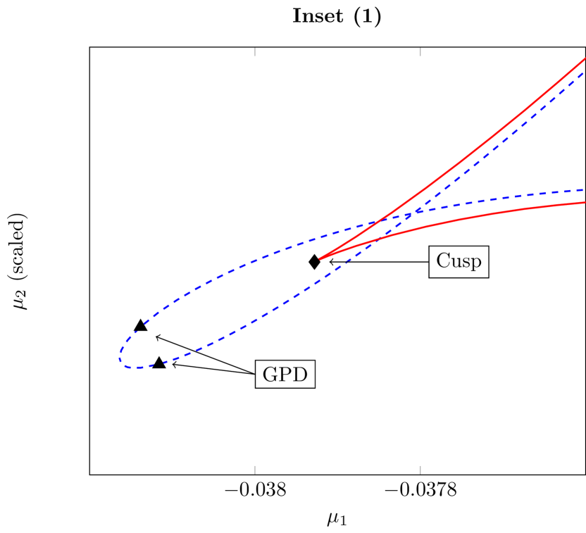
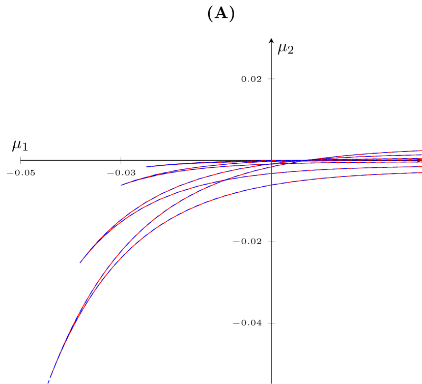
We look for fixed points of map (54) and their various codim 1 curves. The results are similar to that of the scalar model map, except for higher dimensional codim 2 points that exist only in the 3D model map. In Figure 7, we see the PD and LP curves obtained via numerical continuation for a fixed set of parameters: ν=β=0.5,C1=0.8,C2=1.2,α1=0.8,α2=1.3,α3=0.6,α4=1.1formulae-sequence𝜈𝛽0.5formulae-sequencesubscript𝐶10.8formulae-sequencesubscript𝐶21.2formulae-sequencesubscript𝛼10.8formulae-sequencesubscript𝛼21.3formulae-sequencesubscript𝛼30.6subscript𝛼41.1\nu=\beta=0.5,C_{1}=0.8,C_{2}=1.2,\alpha_{1}=0.8,\alpha_{2}=1.3,\alpha_{3}=0.6,\alpha_{4}=1.1 and ϕ1=ϕ2=π/6subscriptitalic-ϕ1subscriptitalic-ϕ2𝜋6\phi_{1}=\phi_{2}=\pi/6. We immediately see similarities with the scalar case. The global structure of these curves is the same as in the scalar case. They form sequences that accumulate onto the primary homoclinic curve asymptotically. The LP ‘horns’ have cusp points and are accompanied by PD curves with/without GPD points (depending on saddle or spring area). All this is expected as the scalar map is a correct asymptotic representation of the 3D model map.
Refer to caption
Refer to caption
Refer to caption
Refer to caption
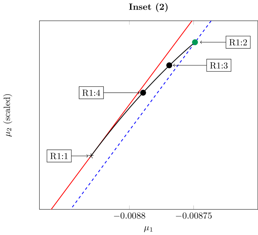
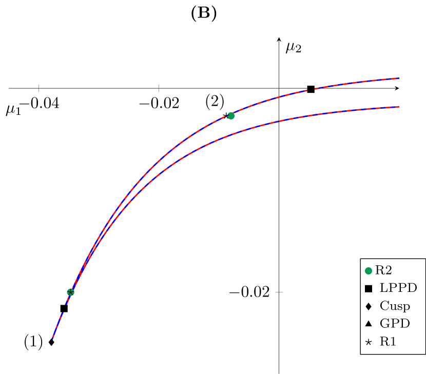
Figure 7: Primary LP (solid red) and PD (dashed blue) curves obtained by numerical continuation for the map (54). The parameters are fixed as ν=0.5𝜈0.5\nu=0.5, β=0.5,C1=0.8,C2=1.2,α1=0.8,α2=1.3,α3=0.6,α4=1.1formulae-sequence𝛽0.5formulae-sequencesubscript𝐶10.8formulae-sequencesubscript𝐶21.2formulae-sequencesubscript𝛼10.8formulae-sequencesubscript𝛼21.3formulae-sequencesubscript𝛼30.6subscript𝛼41.1\beta=0.5,C_{1}=0.8,C_{2}=1.2,\alpha_{1}=0.8,\alpha_{2}=1.3,\alpha_{3}=0.6,\alpha_{4}=1.1 and ϕ1=ϕ2=π/6subscriptitalic-ϕ1subscriptitalic-ϕ2𝜋6\phi_{1}=\phi_{2}=\pi/6. The curves have almost the same global structure as for the 1D map, as can be seen in (A). In (B) one such curve is presented, together with several codim 2 points found along it. In Inset (1) we see the previously described spring area made up by the PD and LP curves. Three codim 2 bifurcation points are observed, two corresponding to the generalised period doubling (GPD) bifurcation and one corresponding to the Cusp bifurcation. In Inset (2) we see the interaction between the 1:2 resonance (R2) point on the PD curve and the 1:1 resonance point (R1) on the LP curve, via the primary NS curve (solid black). On this curve we find two more codimension 2 bifurcation points: 1:3 resonance (R3) and 1:4 resonance (R4).

There are however three main differences with respect to the scalar model map which can be attributed to the higher dimension of the 3D map:

  1. 1.

    Spring and saddle areas may occur differently for the 1D and 3D model maps for the same parameter values. All these points numerically appear to asymptotically approach the 3DL transition point.

  2. 2.

    Along the PD, LP and NS curves we observe many higher dimensional codimension 2 points. These points are R1:1 (Resonance 1:1), R1:2 (Resonance 1:2), LPPD (Fold-Flip), R1:3 (Resonance 1:3), R1:4 (Resonance 1:4).

  3. 3.

    There exists two NS curves in a very small domain between the PD and LP curves. The end points of the NS segment are strong resonance points.

These points appear to numerically approach the origin μ=0𝜇0\mu=0 (3DL transition). The endpoints of the NS curve are points R1 and R2, as can be seen in Figure 7 (B). For a detailed discussion on the various codimension 2 points and their local bifurcation diagrams, see [21].

We did not see a significant difference in behavior of the PD/LP curves upon changing the coefficients αisubscript𝛼𝑖\alpha_{i} and ϕjsubscriptitalic-ϕ𝑗\phi_{j}. This can be attributed to the effect of the corresponding terms in (54) to the dynamics of x4subscript𝑥4x_{4}. These terms are o(xν)𝑜superscriptnorm𝑥𝜈o(\|x\|^{\nu}) in the fixed point equation for x4subscript𝑥4x_{4}.
In Table LABEL:tab:codim2 we present sequences of some of the codimension 2 points found on successive PD/LP curves of Figure 7. These sequences are obtained via detection along PD/LP curves from continuation. GPD and CP points are not reported as they are generally hard to detect along continuations, due to large test function values and absolute gradients. They are approximated in practice by noting where the sign of the scalar GPD test function changes. Note that codimension 2 points such as R1, R2 and LPPD were observed more than once on a single PD/LP curve. In Table LABEL:tab:codim2 we show only one point per curve for each of the different bifurcation points.

Table 1: Cascades of codimension two points numerically obtained during continuation of limit point/period doubling solutions of the 3D map (54). Note that the fixed parameter values are the same as in Figure 7.
LPPD (1) R1 (1) R2 (2)
μ1subscript𝜇1\mu_{1} μ2subscript𝜇2\mu_{2} μ1subscript𝜇1\mu_{1} μ2subscript𝜇2\mu_{2} μ1subscript𝜇1\mu_{1} μ2subscript𝜇2\mu_{2}
555 .9031103.9031superscript103.9031\cdot 10^{-3} 22-2 .4503104.4503superscript104.4503\cdot 10^{-4} 99-9 .9025103.9025superscript103.9025\cdot 10^{-3} 55-5 .1621103.1621superscript103.1621\cdot 10^{-3} 00-0 .0402.0402.0402 00-0 .0423.0423.0423
555 .3053103.3053superscript103.3053\cdot 10^{-3} 11-1 .3752104.3752superscript104.3752\cdot 10^{-4} 88-8 .8301103.8301superscript103.8301\cdot 10^{-3} 22-2 .7386103.7386superscript103.7386\cdot 10^{-3} 00-0 .0347.0347.0347 00-0 .0200.0200.0200
444 .3915103.3915superscript103.3915\cdot 10^{-3} 44-4 .1359105.1359superscript105.1359\cdot 10^{-5} 77-7 .2678103.2678superscript103.2678\cdot 10^{-3} 77-7 .7386104.7386superscript104.7386\cdot 10^{-4} 00-0 .0274.0274.0274 55-5 .0254103.0254superscript103.0254\cdot 10^{-3}
333 .7375103.7375superscript103.7375\cdot 10^{-3} 11-1 .212105.212superscript105.212\cdot 10^{-5} 66-6 .1795103.1795superscript103.1795\cdot 10^{-3} 22-2 .1925104.1925superscript104.1925\cdot 10^{-4} 00-0 .0227.0227.0227 11-1 .3355103.3355superscript103.3355\cdot 10^{-3}
333 .2506103.2506superscript103.2506\cdot 10^{-3} 33-3 .5143106.5143superscript106.5143\cdot 10^{-6} 55-5 .3758103.3758superscript103.3758\cdot 10^{-3} 66-6 .2199105.2199superscript105.2199\cdot 10^{-5} 00-0 .0195.0195.0195 33-3 .6375104.6375superscript104.6375\cdot 10^{-4}
333 .0515103.0515superscript103.0515\cdot 10^{-3} 11-1 .8884106.8884superscript106.8884\cdot 10^{-6} 55-5 .0477103.0477superscript103.0477\cdot 10^{-3} 33-3 .3139105.3139superscript105.3139\cdot 10^{-5} 00-0 .0182.0182.0182 11-1 .9084104.9084superscript104.9084\cdot 10^{-4}
222 .8753103.8753superscript103.8753\cdot 10^{-3} 11-1 .0137106.0137superscript106.0137\cdot 10^{-6} 44-4 .7574103.7574superscript103.7574\cdot 10^{-3} 11-1 .7659105.7659superscript105.7659\cdot 10^{-5} 00-0 .0160.0160.0160 55-5 .288105.288superscript105.288\cdot 10^{-5}
222 .7184103.7184superscript103.7184\cdot 10^{-3} 55-5 .4376107.4376superscript107.4376\cdot 10^{-7} 44-4 .4987103.4987superscript103.4987\cdot 10^{-3} 99-9 .4115106.4115superscript106.4115\cdot 10^{-6} 00-0 .0152.0152.0152 22-2 .7905105.7905superscript105.7905\cdot 10^{-5}
222 .3357103.3357superscript103.3357\cdot 10^{-3} 88-8 .3651108.3651superscript108.3651\cdot 10^{-8} 33-3 .8678103.8678superscript103.8678\cdot 10^{-3} 11-1 .4255106.4255superscript106.4255\cdot 10^{-6} 00-0 .0136.0136.0136 77-7 .7986106.7986superscript106.7986\cdot 10^{-6}

For the scalar map we observed that there exist transitions between spring and saddle areas. These transitions can be explained by observing the appearance and disappearance of GPD points, as they exist generically on the PD loop in a spring area, and do not exist in the case of a saddle area. In the 3D case too, we numerically observe such transitions. However, when there is a spring (saddle) area in the 3D case, it does not imply that the same structure would exist in the 1D map for the same choice of parameters C1subscript𝐶1C_{1} and C2subscript𝐶2C_{2}. This is shown in Figure 8.

Refer to caption
Figure 8: Plots of spring and saddle areas in the scalar map (23) and 3D map (19). In all plots μ2subscript𝜇2\mu_{2} is scaled for convenience. In (A) we see that there exists a saddle area in the 3D case, where GPD points are absent. (B) and (C) are plotted for the same value of C1subscript𝐶1C_{1} and C2subscript𝐶2C_{2}, but with respect to the 3D map (19) and 1D map (23) respectively. We see that the existence of the spring area in the 3D map does not imply the existence of the same in the 1D map. Other parameters fixed as in Figure 7.

4.2 Secondary homoclinic orbits

In this section we analyze a particular type of homoclinic orbits, i.e. secondary homoclinic orbits which – after leaving the saddle along the unstable manifold – make two global turns before returning to the saddle.

We look at the existence of these homoclinic orbits close to the primary homoclinic orbit in (2), upon perturbing parameters μ1subscript𝜇1\mu_{1} and μ2subscript𝜇2\mu_{2}. The existence of the orbits is a codim 1 situation and corresponds to a curve in the (μ1,μ2)subscript𝜇1subscript𝜇2(\mu_{1},\mu_{2})-plane. As before, we look for these curves in the wild case, where ν<1𝜈1\nu<1. In the tame case ν>1𝜈1\nu>1, they do not exist.

Refer to caption
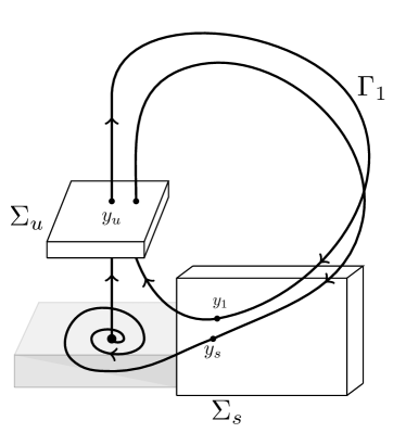
Figure 9: Poincaré map for the secondary homoclinic solution Γ1subscriptΓ1\Gamma_{1}. Upon leaving yusubscript𝑦𝑢y_{u} along the unstable manifold, the corresponding orbit makes two global turns and returns to the origin.

Consider Figure 9. The secondary homoclinic orbit Γ1subscriptΓ1\Gamma_{1} in the locally linearized ODE (2) leaves the point yu=(0,0,0,1)Σusubscript𝑦𝑢0001subscriptΣ𝑢y_{u}=(0,0,0,1)\in\Sigma_{u}, along the unstable manifold and meets ΣssubscriptΣ𝑠\Sigma_{s} at y1=(1,0,1,μ2)subscript𝑦1101subscript𝜇2y_{1}=(1,0,1,\mu_{2}). From this point, the orbit departs again and this time returns along the stable manifold to approach the origin. The orbit crosses ΣssubscriptΣ𝑠\Sigma_{s} at ys=(1,0,1,0)subscript𝑦𝑠1010y_{s}=(1,0,1,0). Using the 3D model map G𝐺G defined by (54), the condition is

G(11μ2)=(110),𝐺11subscript𝜇2110\displaystyle G\left(\begin{array}[]{l}1\\ 1\\ \mu_{2}\end{array}\right)=\left(\begin{array}[]{l}1\\ 1\\ 0\end{array}\right), (61)

which implies

μ2+C1μ2νsin(1βlnμ2)+C2μ2ν+μ1/β=0.subscript𝜇2subscript𝐶1superscriptsubscript𝜇2𝜈1𝛽subscript𝜇2subscript𝐶2superscriptsubscript𝜇2𝜈subscript𝜇1𝛽0\displaystyle\mu_{2}+C_{1}\mu_{2}^{\nu}\sin\left(-\frac{1}{\beta}\ln\mu_{2}\right)+C_{2}\mu_{2}^{\nu+\mu_{1}/\beta}=0. (62)

Let us define

H(μ):=μ2+C1μ2νsin(1βlnμ2)+C2μ2ν+μ1/β.assign𝐻𝜇subscript𝜇2subscript𝐶1superscriptsubscript𝜇2𝜈1𝛽subscript𝜇2subscript𝐶2superscriptsubscript𝜇2𝜈subscript𝜇1𝛽\displaystyle H(\mu):=\mu_{2}+C_{1}\mu_{2}^{\nu}\sin\left(-\frac{1}{\beta}\ln\mu_{2}\right)+C_{2}\mu_{2}^{\nu+\mu_{1}/\beta}. (63)

Note that here μ2subscript𝜇2\mu_{2} must be positive. The shape of H(μ)=0𝐻𝜇0H(\mu)=0 is similar to the curve F(x,μ)=0𝐹𝑥𝜇0F(x,\mu)=0 (from (23)). For positive μ1subscript𝜇1\mu_{1}, it is possible to obtain infinitely many solutions of (62) for μ2subscript𝜇2\mu_{2} sufficiently small. That is not the case when μ1<0subscript𝜇10\mu_{1}<0, as there are only finitely many or no non-trivial solutions for μ2subscript𝜇2\mu_{2} sufficiently small.

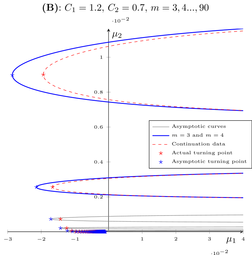
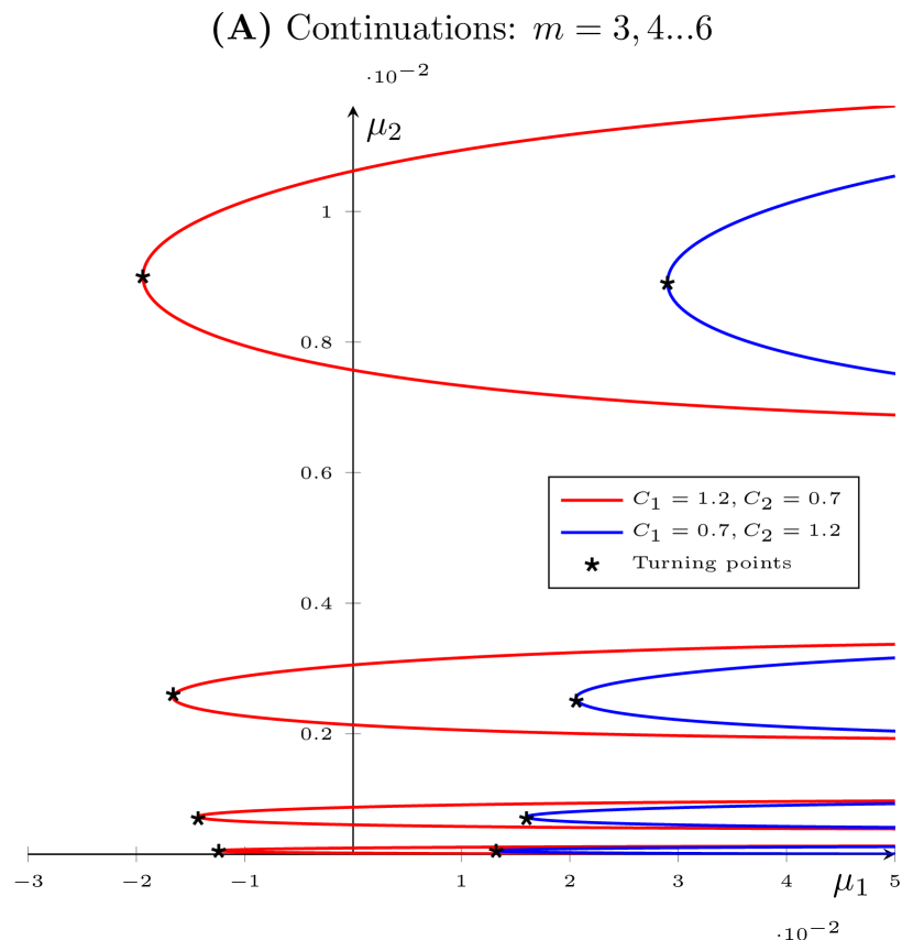
In Figure 10 the non-trivial solutions are continued with respect to the parameters μ1subscript𝜇1\mu_{1} and μ2subscript𝜇2\mu_{2} for two different sets of values of C1subscript𝐶1C_{1} and C2subscript𝐶2C_{2}. We observe three things:

  1. 1.

    There are secondary homoclinic curves which form horizontal parabolas and these ‘parabolas’ approach the primary homoclinic curve μ2=0subscript𝜇20\mu_{2}=0 asymptotically.

  2. 2.

    These ‘parabolas’ possess turning points where the two upper and lower secondary homoclinic branches merge. The sequence of turning points obtained from successive ‘parabolas’ appears to approach the origin asymptotically.

  3. 3.

    For different values of C1subscript𝐶1C_{1} and C2subscript𝐶2C_{2}, the sequence of turning points is located strictly either in the first or second quadrant.
Refer to caption
Refer to caption
Refer to caption
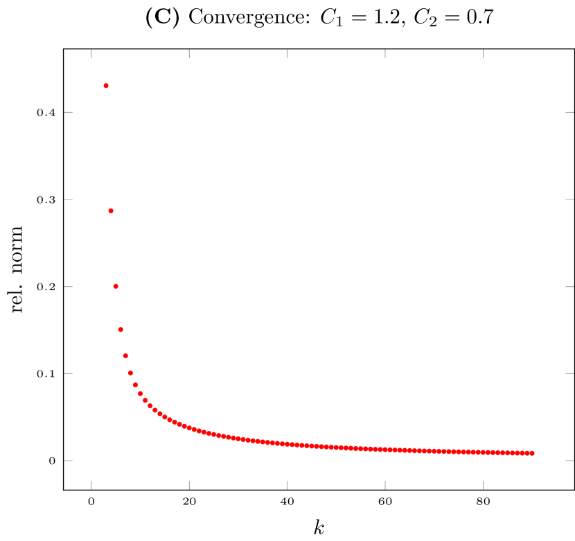
Figure 10: Solutions of (62) in (μ1,μ2)subscript𝜇1subscript𝜇2(\mu_{1},\mu_{2})-space. In (A), ‘parabolas’ are obtained via continuation in Matcont, for two sets of parameter values. The exact turning points (in black) are obtained by Netwon iterations. In (B), exact curves are plotted along with asymptotic curves. In (C), we plot relative norm differences between asymptotic and exact turning points.

4.3 Asymptotics of secondary homoclinics

The observations above can be explained to some extent by asymptotic expressions for the parabolas and the corresponding turning points.

4.3.1 ‘Parabolas’

Noticing μ2>0subscript𝜇20\mu_{2}>0, let

1βlnμ2=2πm+θ,1𝛽subscript𝜇22𝜋𝑚𝜃\displaystyle-\frac{1}{\beta}\ln\mu_{2}=2\pi m+\theta, (64)

for large m𝑚m\in\mathbb{N} and θ(0,2π)𝜃02𝜋\theta\in(0,2\pi). On dividing both sides by μ2ν0superscriptsubscript𝜇2𝜈0\mu_{2}^{\nu}\neq 0 and using the above parametrization for μ2subscript𝜇2\mu_{2}, (62) becomes

eβ(1ν)(πm+θ)+C1sinθ+C2eμ1(πm+θ)=0.superscript𝑒𝛽1𝜈𝜋𝑚𝜃subscript𝐶1𝜃subscript𝐶2superscript𝑒subscript𝜇1𝜋𝑚𝜃0\displaystyle e^{-\beta(1-\nu)(\pi m+\theta)}+C_{1}\sin\theta+C_{2}e^{-\mu_{1}(\pi m+\theta)}=0. (65)

On simplifying, we get

sinθ=C2C1e2πμ1m(1μ1θ+O(μ12))+O(eαm),𝜃subscript𝐶2subscript𝐶1superscript𝑒2𝜋subscript𝜇1𝑚1subscript𝜇1𝜃𝑂superscriptsubscript𝜇12𝑂superscript𝑒𝛼𝑚\sin\theta=-\frac{C_{2}}{C_{1}}e^{-2\pi\mu_{1}m}(1-\mu_{1}\theta+O(\mu_{1}^{2}))+O(e^{-\alpha m}), (66)

where α=2πβ(1ν)𝛼2𝜋𝛽1𝜈\alpha=2\pi\beta(1-\nu). For large m𝑚m and negative μ1subscript𝜇1\mu_{1}, a solution θ𝜃\theta exists only for small |μ1|subscript𝜇1|\mu_{1}|. Thus we get two solutions θ𝜃\theta from (66),

θ1=θ0m+δi1(2π)+O(1/m),θ2=πθ0m+O(1/m),subscript𝜃1subscriptsuperscript𝜃𝑚0subscript𝛿𝑖12𝜋𝑂1𝑚subscript𝜃2𝜋subscriptsuperscript𝜃𝑚0𝑂1𝑚\begin{array}[]{l}\theta_{1}=\theta^{m}_{0}+\delta_{i1}(2\pi)+O(1/m),\\ \theta_{2}=\pi-\theta^{m}_{0}+O(1/m),\end{array} (67)

where

θ0m:=arcsin(C2C1e2πμ1m),assignsubscriptsuperscript𝜃𝑚0subscript𝐶2subscript𝐶1superscript𝑒2𝜋subscript𝜇1𝑚\theta^{m}_{0}:=\arcsin\left(-\frac{C_{2}}{C_{1}}e^{-2\pi\mu_{1}m}\right),

the index i=sign(C2)𝑖signsubscript𝐶2i=-{\rm sign}(C_{2}) and δijsubscript𝛿𝑖𝑗\delta_{ij} is the Kronecker delta. Thus the expressions for two ‘half-parabolas’ are

{μ2(m,1)=eβ(2πm+θ0m+δi1(2π))(1+O(1/m)),μ2(m,2)=eβ(2πm+πθ0m)(1+O(1/m)).casessuperscriptsubscript𝜇2𝑚1superscript𝑒𝛽2𝜋𝑚subscriptsuperscript𝜃𝑚0subscript𝛿𝑖12𝜋1𝑂1𝑚missing-subexpressionsuperscriptsubscript𝜇2𝑚2superscript𝑒𝛽2𝜋𝑚𝜋subscriptsuperscript𝜃𝑚01𝑂1𝑚missing-subexpression\left\{\begin{array}[]{ll}\mu_{2}^{(m,1)}=e^{-\beta(2\pi m+\theta^{m}_{0}+\delta_{i1}(2\pi))}(1+O(1/m)),\\ \mu_{2}^{(m,2)}=e^{-\beta(2\pi m+\pi-\theta^{m}_{0})}(1+O(1/m)).\end{array}\right. (68)

Taking derivative with respect to θ𝜃\theta in (66) gives

cosθ=C2C1e2πμ1m(μ1+O(μ12))+O(eαm).𝜃subscript𝐶2subscript𝐶1superscript𝑒2𝜋subscript𝜇1𝑚subscript𝜇1𝑂superscriptsubscript𝜇12𝑂superscript𝑒𝛼𝑚\cos\theta=\frac{C_{2}}{C_{1}}e^{-2\pi\mu_{1}m}(\mu_{1}+O(\mu_{1}^{2}))+O(e^{-\alpha m}). (69)

Solving (66) and (69) together gives the condition for turning points. Using the two conditions gives,

C22C12e4πμ1m(1+O(μ1))+O(eαm)=1.superscriptsubscript𝐶22superscriptsubscript𝐶12superscript𝑒4𝜋subscript𝜇1𝑚1𝑂subscript𝜇1𝑂superscript𝑒𝛼𝑚1\frac{C_{2}^{2}}{C_{1}^{2}}e^{-4\pi\mu_{1}m}(1+O(\mu_{1}))+O(e^{-\alpha m})=1. (70)

From this we get μ1subscript𝜇1\mu_{1},

μ1=14πm[ln(C22C12)+O(1m)],subscript𝜇114𝜋𝑚delimited-[]superscriptsubscript𝐶22superscriptsubscript𝐶12𝑂1𝑚\mu_{1}=\frac{1}{4\pi m}\left[\ln\left(\frac{C_{2}^{2}}{C_{1}^{2}}\right)+O\left(\frac{1}{m}\right)\right], (71)

which is the same as the condition

sin2θ=1.superscript2𝜃1\sin^{2}\theta=1. (72)

Thus the sequence of turning points is given by

(μ1(m)μ2(m))=(1(4πm)(ln(C22C12)+O(1m))eβ(2πm+θ0)(1+O(1m))),superscriptsubscript𝜇1𝑚superscriptsubscript𝜇2𝑚14𝜋𝑚superscriptsubscript𝐶22superscriptsubscript𝐶12𝑂1𝑚superscript𝑒𝛽2𝜋𝑚subscript𝜃01𝑂1𝑚\displaystyle\left(\begin{array}[]{l}\mu_{1}^{(m)}\\ \mu_{2}^{(m)}\end{array}\right)=\left(\begin{array}[]{l}\frac{1}{(4\pi m)}\left(\ln\left(\frac{C_{2}^{2}}{C_{1}^{2}}\right)+O\left(\frac{1}{m}\right)\right)\\ e^{-\beta(2\pi m+\theta_{0})}\left(1+O\left(\frac{1}{m}\right)\right)\end{array}\right), (77)

where

θ0={π/2,ifC2<0,3π/2,ifC2>0.subscript𝜃0cases𝜋2ifsubscript𝐶203𝜋2ifsubscript𝐶20\theta_{0}=\left\{\begin{array}[]{ll}\pi/2,&\textnormal{if}\ C_{2}<0,\\ 3\pi/2,&\textnormal{if}\ C_{2}>0.\end{array}\right. (78)

We summarize the results in the following lemma.

Lemma 4.1.

For the 3D model map G𝐺G defined by (19)19(\ref{eq:3Dmap}), the condition

G(11μ2)=(110)𝐺11subscript𝜇2110\displaystyle G\left(\begin{array}[]{l}1\\ 1\\ \mu_{2}\end{array}\right)=\left(\begin{array}[]{l}1\\ 1\\ 0\end{array}\right) (85)

defines in a neighbourhood of the origin of the (μ1,μ2)subscript𝜇1subscript𝜇2(\mu_{1},\mu_{2})-plane, an infinite sequence of ‘parabolas’ Homm(2),m,𝐻𝑜subscriptsuperscript𝑚2𝑚𝑚Hom^{(2)}_{m},~{}~{}m\in\mathbb{N}, that accumulate onto the half axis μ2=0subscript𝜇20\mu_{2}=0 with μ10subscript𝜇10\mu_{1}\geq 0. Each parabola is formed by two branches with the following asymptotic representation:

{μ2(m,1)=eβ0(2πm+θ0m+δi1(2π))(1+O(1m)),μ2(m,2)=eβ0(2πm+πθ0m)(1+O(1m)),casessuperscriptsubscript𝜇2𝑚1superscript𝑒subscript𝛽02𝜋𝑚subscriptsuperscript𝜃𝑚0subscript𝛿𝑖12𝜋1𝑂1𝑚missing-subexpressionsuperscriptsubscript𝜇2𝑚2superscript𝑒subscript𝛽02𝜋𝑚𝜋subscriptsuperscript𝜃𝑚01𝑂1𝑚missing-subexpression\left\{\begin{array}[]{ll}\mu_{2}^{(m,1)}=e^{-\beta_{0}(2\pi m+\theta^{m}_{0}+\delta_{i1}(2\pi))}\left(1+O\left(\frac{1}{m}\right)\right),\\ \mu_{2}^{(m,2)}=e^{-\beta_{0}(2\pi m+\pi-\theta^{m}_{0})}\left(1+O\left(\frac{1}{m}\right)\right),\end{array}\right. (86)

where

θ0m:=arcsin(C20C10e2πμ1m).assignsubscriptsuperscript𝜃𝑚0subscriptsuperscript𝐶02subscriptsuperscript𝐶01superscript𝑒2𝜋subscript𝜇1𝑚\theta^{m}_{0}:=\arcsin\left(-\frac{C^{0}_{2}}{C^{0}_{1}}e^{-2\pi\mu_{1}m}\right).

These branches meet at a sequence of turning points Tm(2)subscriptsuperscript𝑇2𝑚T^{(2)}_{m}, which converges to the origin of the (μ1,μ2)subscript𝜇1subscript𝜇2(\mu_{1},\mu_{2})-plane and is given by

Tm(2)=(μ1(m)μ2(m))=(1(4πm)(ln[(C20)2(C10)2]+O(1m))eβ0(πm+π/2+δi1(2π))(1+O(1m))).subscriptsuperscript𝑇2𝑚superscriptsubscript𝜇1𝑚superscriptsubscript𝜇2𝑚14𝜋𝑚superscriptsubscriptsuperscript𝐶022superscriptsubscriptsuperscript𝐶012𝑂1𝑚superscript𝑒subscript𝛽0𝜋𝑚𝜋2subscript𝛿𝑖12𝜋1𝑂1𝑚T^{(2)}_{m}=\left(\begin{array}[]{l}\mu_{1}^{(m)}\\ \mu_{2}^{(m)}\end{array}\right)=\left(\begin{array}[]{l}\frac{1}{(4\pi m)}\left(\ln\left[\frac{(C^{0}_{2})^{2}}{(C^{0}_{1})^{2}}\right]+O\left(\frac{1}{m}\right)\right)\\ e^{-\beta_{0}(\pi m+\pi/2+\delta_{i1}(2\pi))}\left(1+O\left(\frac{1}{m}\right)\right)\end{array}\right). (87)

5 Interpretation for the original ODE system

Let us consider the original 4D system (2) in the linearizing coordinates near the equilibrium, the geometric construction in Figure 4 and the full 3D map ΠΠ\Pi defined by (13).

Fixed points of this map ΠΠ\Pi in ΣssubscriptΣ𝑠\Sigma_{s} correspond to periodic orbits, thus period doubling and fold bifurcations of these fixed points of this map correspond to the same bifurcations of periodic orbits in the original ODE system.

The second iterate of the map (13), such that μ2>0subscript𝜇20\mu_{2}>0, defines an orbit in the original system (2) which makes an extra global excursion before returning to ΣusubscriptΣ𝑢\Sigma_{u}. Starting at a point in the unstable 1D manifold of the equilibrium and letting the third component of the image to zero, implies that we consider an orbit of the ODE that departs along the unstable manifold and returns along the stable manifold back to the saddle. This orbit is therefore a secondary homoclinic orbit near the primary one.

Using Lemmas 3.1 and 87 we are now able to formulate our main results in terms of the original 4D ODE near the 3DL-homoclinic transition. It follows from the fact that taking into account the o(xν)𝑜superscriptnorm𝑥𝜈o(\|x\|^{\nu})-term in (13) does not alter the leading terms in all expressions, which further implies that given asymptotics are the same for the truncated map (54) and full 3D return map (13).

Theorem 5.1.

Consider a smooth 4D ODE system depending on two parameters

x˙=f(x,α),x4,α2.formulae-sequence˙𝑥𝑓𝑥𝛼formulae-sequence𝑥superscript4𝛼superscript2\dot{x}=f(x,\alpha),~{}~{}x\in\mathbb{R}^{4},~{}\alpha\in\mathbb{R}^{2}. (88)

Suppose that at α=0𝛼0\alpha=0 the system (88)88(\ref{4DODE}) satisfies the following assumptions:

  1. (B.1) The eigenvalues of the linearisation at the critical 3DL equilibrium x=0𝑥0x=0 are

    δ0,δ0±iω0 and ϵ0,subscript𝛿0plus-or-minussubscript𝛿0𝑖subscript𝜔0 and subscriptitalic-ϵ0\delta_{0},\delta_{0}\pm i\omega_{0}\textnormal{ and }\epsilon_{0},

    where δ0<0,ω0>0formulae-sequencesubscript𝛿00subscript𝜔00\delta_{0}<0,\omega_{0}>0, ϵ0>0subscriptitalic-ϵ00\epsilon_{0}>0 and σ0=δ0+ϵ0>0subscript𝜎0subscript𝛿0subscriptitalic-ϵ00\sigma_{0}=\delta_{0}+\epsilon_{0}>0.

  2. (B.2) There exists a primary homoclinic orbit Γ0subscriptΓ0\Gamma_{0} to this 3DL equilibrium.

  3. (B.3) The homoclinic orbit Γ0subscriptΓ0\Gamma_{0} satisfies the following genericity condition: The normalized tangent vector to Γ0subscriptΓ0\Gamma_{0} has nonzero projections to both the 1D eigenspace corresponding to the real eigenvalue δ0subscript𝛿0\delta_{0} and to the 2D eigenspace corresponding to the complex eigenvalues δ0±iω0plus-or-minussubscript𝛿0𝑖subscript𝜔0\delta_{0}\pm i\omega_{0}, when approaching the equilibrium at t𝑡t\rightarrow\infty.

Then, in addition to the primary homoclinic curve Hom(1)𝐻𝑜superscript𝑚1Hom^{(1)}, the bifurcation set of (88)88(\ref{4DODE}) in a neighborhood of α=0𝛼0\alpha=0 generically contains the following elements:::

  1. (i)

    An infinite number of fold bifurcation curves LPn(1),n,𝐿superscriptsubscript𝑃𝑛1𝑛LP_{n}^{(1)},n\in\mathbb{N}, along which limit cycles with multiplier +11+1 exist making one global excursion and a number of small turns near the equilibrium. These curves accumulate to the saddle-focus part of the primary homoclinic curve. Each curve resembles a ‘horn’ consisting of two branches that meet at a cusp point CPn(1)𝐶superscriptsubscript𝑃𝑛1CP_{n}^{(1)}. The sequence of cusp points converges to α=0𝛼0\alpha=0.

  2. (ii)

    An infinite number of period-doubling bifurcation curves PDn(1),n,𝑃superscriptsubscript𝐷𝑛1𝑛PD_{n}^{(1)},n\in\mathbb{N}, along which limit cycles with multiplier 11-1 exist making one global excursion and a number of small turns near the equilibrium. Away from the cusp points CPn(1)𝐶superscriptsubscript𝑃𝑛1CP_{n}^{(1)}, these period-doubling curves have the same asymptotic properties as the fold bifurcation curves LPn(1)𝐿superscriptsubscript𝑃𝑛1LP_{n}^{(1)}. These period-doubling curves could either be smooth or have self-intersections developing small loops around the corresponding cusp points.

  3. (iii)

    An infinite number of secondary homoclinic curves Homm(2),m,𝐻𝑜superscriptsubscript𝑚𝑚2𝑚Hom_{m}^{(2)},m\in\mathbb{N}, along which the equilibrium has homoclinic orbits making two global excursions and a number of turns near the equilibrium after the first global excursion. These curves also accumulate to the saddle-focus part of the primary homoclinic curve. Each curve resembles a ‘parabola’ and the sequence of turning points converges to α=0𝛼0\alpha=0.

Refer to caption
Figure 11: A sketch of two consecutive LP horns from Theorem 5.1. The saddle-focus part of Hom(1)𝐻𝑜superscript𝑚1Hom^{(1)} branch is drawn in blue.

Part (i) of Theorem 5.1 is illustrated in Figure 11. Notice that LPn(1)𝐿subscriptsuperscript𝑃1𝑛LP^{(1)}_{n} curves can intersect the primary homoclinic branch Hom(1)𝐻𝑜superscript𝑚1Hom^{(1)} either at saddle points (Figure 11(a)) or at saddle-focus points (Figure 11(b)). In terms of the 1D (or 3D) model map these cases correspond to C20>0subscriptsuperscript𝐶020C^{0}_{2}>0 and C10>C20subscriptsuperscript𝐶01subscriptsuperscript𝐶02C^{0}_{1}>C^{0}_{2} or C10<C20subscriptsuperscript𝐶01subscriptsuperscript𝐶02C^{0}_{1}<C^{0}_{2}, respectively. See equation (35).

Refer to caption
Figure 12: A sketch of two consecutive secondary homoclinic curves from Theorem 5.1. The saddle-focus part of Hom(1)𝐻𝑜superscript𝑚1Hom^{(1)} branch is drawn in blue.

Part (iii) of Theorem 5.1 is illustrated in Figure 12. Notice that the turning points of the secondary homoclinic curves Homm(2)𝐻𝑜superscriptsubscript𝑚𝑚2Hom_{m}^{(2)} approach the 3DL transition point on Hom(1)𝐻𝑜superscript𝑚1Hom^{(1)} either along its saddle part (Figure 12(a)) or its saddle-focus part (Figure 12(b)). In terms of the 2D (or 3D) model map these cases also correspond to C10>|C20|subscriptsuperscript𝐶01subscriptsuperscript𝐶02C^{0}_{1}>|C^{0}_{2}| or C10<|C20|subscriptsuperscript𝐶01subscriptsuperscript𝐶02C^{0}_{1}<|C^{0}_{2}|, respectively. See equation (71).

Our numerical analysis of the truncated model 3D map (19) also reveals NS curves in very small domains between the PD- and LP-curves. These curves correspond to torus bifurcation of cycles in the ODE system and do not exist for all combinations of (C10,C20)subscriptsuperscript𝐶01subscriptsuperscript𝐶02(C^{0}_{1},C^{0}_{2}). The end points of the NS segment are strong resonance points. There are other codimension 2 points, i.e. GPD and LPPD. All these points should also be present in the generic ODE system and should form sequences that converge to the 3DL-transition point.

6 The Lorenz-Stenflo model

In this section we review the Lorenz-Stenflo model and discuss the presence of the 3DL-transition.

The Lorenz-Stenflo (LS) equations are a generalization of the well known Lorenz equations [22], that describe low-frequency, short-wavelength acoustic-gravity perturbations in the atmosphere with additional dependence on the earth’s rotation. The equations are as follows:

{x˙=σ(yx)+su,y˙=rxxzy,z˙=xybz,u˙=xσu,cases˙𝑥𝜎𝑦𝑥𝑠𝑢˙𝑦𝑟𝑥𝑥𝑧𝑦˙𝑧𝑥𝑦𝑏𝑧˙𝑢𝑥𝜎𝑢\left\{\begin{array}[]{rcl}\dot{x}&=&\sigma(y-x)+su,\\ \dot{y}&=&rx-xz-y,\\ \dot{z}&=&xy-bz,\\ \dot{u}&=&-x-\sigma u,\end{array}\right. (89)

where σ𝜎\sigma is the Prandtl number, r𝑟r is a generalized Rayleigh parameter, b𝑏b is a positive parameter and s𝑠s is a new parameter dependent on the Earth’s rotation [23]. Setting s=0𝑠0s=0 reduces the first three equations in (90) back to the original Lorenz model.

System (89) possesses 2subscript2\mathbb{Z}_{2}-symmetry, and has one or three equilibria (the trivial equilibrium exists always). The system exhibits a wild 3DL transition, but the corresponding PD and LP curves are difficult to resolve due to highly contractive properties close to the transition, caused by large real parts of the eigenvalues at the trivial equilibrium.

To overcome this, we perturb the system to get:

{x˙=σ(yx)+su,y˙=rxxzy+ϵ𝟏𝒛,z˙=xybz,u˙=xσu+ϵ𝟐𝒚,cases˙𝑥𝜎𝑦𝑥𝑠𝑢˙𝑦𝑟𝑥𝑥𝑧𝑦subscriptbold-italic-ϵ1𝒛˙𝑧𝑥𝑦𝑏𝑧˙𝑢𝑥𝜎𝑢subscriptbold-italic-ϵ2𝒚\left\{\begin{array}[]{rcl}\dot{x}&=&\sigma(y-x)+su,\\ \dot{y}&=&rx-xz-y+\boldsymbol{\epsilon_{1}z},\\ \dot{z}&=&xy-bz,\\ \dot{u}&=&-x-\sigma u+\boldsymbol{\epsilon_{2}y},\end{array}\right. (90)

where the bold expressions are perturbation terms. This system is not 2subscript2\mathbb{Z}_{2} symmetric anymore but still has a trivial equilibrium for all parameter values. We are not aware of any physical interpretation of the added terms.
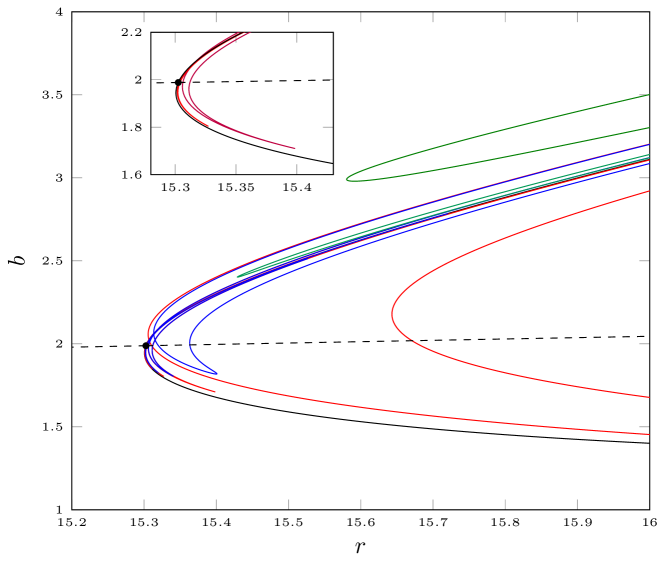
Refer to caption
Figure 13: Bifurcation curves near a wild 3DL transition in the (b,r)𝑏𝑟(b,r)-plane: cyclic folds (red), period-doublings (blue), primary homoclinic (black), 3DL equilibrium transition (dashed black) and secondary homoclinics (green).

In Figure 13 we see a wild 3DL transition along the primary homoclinic curve (black) in the perturbed LS system (90) with

σ=1,s=33,ϵ1=0.1,ϵ2=0.3.formulae-sequence𝜎1formulae-sequence𝑠33formulae-sequencesubscriptitalic-ϵ10.1subscriptitalic-ϵ20.3\sigma=1,\ s=33,\ \epsilon_{1}=0.1,\ \epsilon_{2}=0.3.

The 3DL-transition point is located at

(r,b)(15.302531,1.9884).𝑟𝑏15.3025311.9884(r,b)\approx(15.302531,1.9884).

The corresponding eigenvalues are δ0±iω0,δ0plus-or-minussubscript𝛿0𝑖subscript𝜔0subscript𝛿0\delta_{0}\pm i\omega_{0},\delta_{0}, and ϵ0subscriptitalic-ϵ0\epsilon_{0} with δ01.9884,ω06.2265,ϵ02.7769formulae-sequencesubscript𝛿01.9884formulae-sequencesubscript𝜔06.2265subscriptitalic-ϵ02.7769\delta_{0}\approx-1.9884,\omega_{0}\approx 6.2265,\epsilon_{0}\approx 2.7769.

We clearly see PD (blue) and LP (red) curves accumulating onto the primary homoclinic curve according to the theory. The PD curve within each ‘horn’ forms a saddle area. The secondary homoclinic curves (green) form ‘parabolas’ on one side of the primary homoclinic curve as expected. The curve of trivial equilibria with a 3D stable eigenspace is shown as a dashed line. The cusp points on each LP horn forms a sequence, and asymptotically approach the 3DL point at the intersection of the black curve with the dashed line. The inset shows only the LP horns. For this model the bifurcation curves have been computed using matcont [24] also based on [25, 26].

The 3DL-transition with the associated bifurcation structure exists also in the original 2subscript2\mathbb{Z}_{2} symmetric system (89). However, its bifurcation diagram will include additional bifurcation curves related to (symmetric) cycles and heteroclinic orbits. This will make the whole picture more complicated than in Figure 13.

7 Discussion

We have studied bifurcation diagrams of 4D two-parameter ODEs having at some critical parameter values a homoclinic orbit to an hyperbolic equilibrium with one simple unstable eigenvalue and three simple stable eigenvalues (one real and a complex-conjugate pair). We focused on the case, when a transition from a saddle homoclinic orbit to Shilnikov’s wild saddle-focus homoclinic orbit takes place at the critical parameter values. Similar to the 3D Belyakov’s saddle to wild saddle-focus homoclinic transition, we found infinite sequences of codim 1 bifurcations curves related to limit cycles (i.e., folds and period-doublings) and secondary homoclinic orbits accumulating on the primary (wild) saddle-focus homoclinic branch. However, there is a striking difference between these two cases. While in the standard Belyakov case all bifurcation curves approach the codim 2 point in the parameter plane tangentially to the saddle-focus homoclinic curve (having actually tangency of infinite order) and form ‘bunches’, in the considered 3DL case neither of them approaches the codim 2 point. Instead, they form sequences of ‘horns’ with cusps and other codim 2 bifurcation points, or ‘parabolas’. The sequences of codim 2 points and parabola tops indeed converge to the studied homoclinic 3DL point. In a sense, the bifurcation diagram for the considered 3DL-transition resembles more another codim 2 homoclinic bifurcation studied by Belyakov: A transition from tame to wild saddle-focus homoclinic orbit in 3D ODEs, when the saddle quantity vanishes [27]. In that case, fold bifurcation curves for cycles also have cusp points accumulating to the transition point, while the secondary homoclinic curves look like ‘parabolas’ with tops tending to the transition point. The exact source of this similarity remains a mystery but might be related to the simplicity of all eigenvalues in both cases.

The C1superscript𝐶1C^{1}-linearisation theorem used to derive the Poincaré return map (13) permits to employ only the first-order partial derivatives of this map. This was sufficient to derive asymptotics for the fold and period-doubling bifurcations of the primary limit cycles, as well as those for the secondary homoclinic orbits. However, to verify nondegeneracy conditions for LP and PD bifurcations and to detect codim 2 points, one would need higher-order partial derivatives of the return map ΠΠ\Pi. Their existence can be guaranteed by using the Cksuperscript𝐶𝑘C^{k}-linearisation near the equilibrium with sufficiently big k>1𝑘1k>1. This exists generically, if one imposes a finite number of low-order non-resonance conditions on the real parts of the eigenvalues of the equilibrium (see [28]). However, it looks ptobable that one can avoid such extra conditions by careful analysis of the local flow near the equilibrium in the spirit of [14, Sec. 2.8].

Clearly, 3DL-transitions are also possible in higher phase dimensions. The developed theory can be applied to such cases via a reduction to a four-dimensional homoclinic center-manifold [16, 15, 13] that exists near the bifurcation. However, also here some ‘gap’ conditions should be imposed on the eigenvalues of the critical equilibrium to guarantee more than C1superscript𝐶1C^{1} smoothness of the homoclinic center manifold. Whether one can avoid using the homoclinic center manifolds is also unclear.

Despite two above mentioned smoothness issues, we can conclude that, at least for a large open set of smooth ODEs, the 3DL homoclinic transition implies the complicated bifurcation structure described in the present paper.

An interesting challenge would be to prove analytically the existence of infinite sequences of generalized period-doubling points and strong resonances (see Figure 7), at least for the truncated 3D model map (19).

References

References

  • [1] V. I. Arnold, V. S. Afrajmovich, Yu. S. Il’yashenko, and L. P. Shil’nikov. Dynamical Systems 5: Bifurcation Theory and Catastrophe Theory. Springer-Verlag, Berlin, 1999.
  • [2] Yu. Ilyashenko and Weigu Li. Nonlocal Bifurcations, volume 66 of Mathematical Surveys and Monographs. American Mathematical Society, Providence, RI, 1999.
  • [3] L. P. Shilnikov, A. L. Shilnikov, D. Turaev, and L. O. Chua. Methods of Qualitative Theory in Nonlinear Dynamics. Part II, volume 5 of World Scientific Series on Nonlinear Science. Series A: Monographs and Treatises. World Scientific Publishing Co., Inc., River Edge, NJ, 2001.
  • [4] A. J. Homburg and B. Sandstede. Homoclinic and heteroclinic bifurcations in vector fields. Handbook of Dynamical Systems, 3(C):379–524, 2010.
  • [5] L. P. Shil’nikov. A case of the existence of a denumerable set of periodic motions. Dokl. Akad. Nauk SSSR, 160:558–561, 1965.
  • [6] V. S. Afraimovich, S. V. Gonchenko, L. M. Lerman, A. L. Shil’nikov, and D. V. Turaev. Scientific heritage of L. P. Shilnikov. Regul. Chaotic Dyn., 19(4):435–460, 2014.
  • [7] S. V. Gonchenko, D. V. Turaev, P. Gaspard, and G. Nicolis. Complexity in the bifurcation structure of homoclinic loops to a saddle-focus. Nonlinearity, 10(2):409–423, 1997.
  • [8] A. R. Champneys and Yu. A. Kuznetsov. Numerical detection and continuation of codimension-two homoclinic bifurcations. Internat. J. Bifur. Chaos Appl. Sci. Engrg., 4(4):785–822, 1994.
  • [9] Yu. A. Kuznetsov. Impulses of a complicated form in models of nerve conduction. Selecta Math., 13(2):127–142, 1994. [Translation from Mathematics and Modeling, Akad. Nauk SSSR, Nauchn. Tsentr Biol. Issled., Pushchino, 1990, pp. 208–222].
  • [10] Yu. A. Kuznetsov, O. De Feo, and S. Rinaldi. Belyakov homoclinic bifurcations in a tritrophic food chain model. SIAM J. Appl. Math., 62(2):462–487, 2001.
  • [11] L. A. Belyakov. The bifurcation set in a system with a homoclinic saddle curve. Mat. Zametki, 28(6):911–922, 962, 1980. [in Russian; English translation: Math. Notes 28(5-6): 910–916, 1981].
  • [12] H. G. E. Meijer and S. Coombes. Travelling waves in a neural field model with refractoriness. J. Math. Biol., 68(5):1249–1268, 2014.
  • [13] A. J. Homburg. Global aspects of homoclinic bifurcations of vector fields. Mem. Amer. Math. Soc., 121(578):viii+128, 1996.
  • [14] L. P. Shil’nikov, A. L. Shil’nikov, D. V. Turaev, and L. O. Chua. Methods of Qualitative Theory in Nonlinear Dynamics. Part I, volume 4 of World Scientific Series on Nonlinear Science. Series A: Monographs and Treatises. World Scientific Publishing Co., Inc., River Edge, NJ, 1998.
  • [15] M. V. Shashkov and D. V. Turaev. An existence theorem of smooth nonlocal center manifolds for systems close to a system with a homoclinic loop. J. Nonlinear Sci., 9(5):525–573, 1999.
  • [16] B. Sandstede. Center manifolds for homoclinic solutions. J. Dynam. Differential Equations, 12(3):449–510, 2000.
  • [17] C. Mira and J.-P. Carcassès. On the “crossroad area–saddle area” and “crossroad area–spring area” transitions. Internat. J. Bifur. Chaos Appl. Sci. Engrg., 1(3):641–655, 1991.
  • [18] G. R. Belitskii. Normal Forms, Invariants, and Local Mappings. Naukova Dumka, Kiev, 1979. [in Russian].
  • [19] W. Govaerts, R. Khoshsiar Ghaziani, Yu. A. Kuznetsov, and H. G. E. Meijer. Numerical methods for two-parameter local bifurcation analysis of maps. SIAM Journal on Scientific Computing, 29(6):2644–2667, 2007.
  • [20] N. Neirynck, B. Al-Hdaibat, W. Govaerts, Yu. A. Kuznetsov, and H.G.E. Meijer. Using MatContM in the study of a nonlinear map in economics. Journal of Physics: Conference Series, 692(1):012013, 2016.
  • [21] Yu. A. Kuznetsov. Elements of Applied Bifurcation Theory, volume 112 of Applied Mathematical Sciences. Springer-Verlag, New York, third edition, 2004.
  • [22] E. N. Lorenz. Deterministic nonperiodic flow. Journal of the Atmospheric Sciences, 20(2):130–141, 1963.
  • [23] L. Stenflo. Generalized Lorenz equations for acoustic-gravity waves in the atmosphere. Physica Scripta, 53(1):83, 1996.
  • [24] A. Dhooge, W. Govaerts, and Yu. A. Kuznetsov. Matcont: A MATLAB package for numerical bifurcation analysis of ODEs. ACM Trans. Math. Softw., 29(2):141–164, June 2003.
  • [25] A. R. Champneys, Yu. A. Kuznetsov, and B. Sandstede. A numerical toolbox for homoclinic bifurcation analysis. Internat. J. Bifur. Chaos Appl. Sci. Engrg., 6(5):867–887, 1996.
  • [26] V. De Witte, W. Govaerts, Yu. A. Kuznetsov, and M. Friedman. Interactive initialization and continuation of homoclinic and heteroclinic orbits in MATLAB. ACM Trans. Math. Software, 38(3):Art. 18, 34, 2012.
  • [27] L.A. Belyakov. Bifurcations of systems with a homoclinic curve of the saddle-focus with a zero saddle value. Mat. Zametki, 36(5):681–689, 798, 1984. [in Russian; English translation: Math. Notes 36(5-6): 838 - 843, 1985].
  • [28] I. U. Bronstein and A. Ya. Kopanskiĭ. Smooth invariant manifolds and normal forms, volume 7 of World Scientific Series on Nonlinear Science. Series A: Monographs and Treatises. World Scientific Publishing Co., Inc., River Edge, NJ, 1994.