Reconstruction of Brain Activity from EEG/MEG
Using MV-PURE Framework

Abstract

We consider the problem of reconstruction of brain activity from electroencephalography (EEG) or magnetoencephalography (MEG) using spatial filtering (beamforming). We propose spatial filters which are based on the minimum-variance pseudo-unbiased reduced-rank estimation (MV-PURE) framework. They come in two flavours, depending whether the EEG/MEG forward model considers explicitly “interfering activity”, understood as brain’s electrical activity originating from brain areas other than regions of interest which is recorded at EEG/MEG sensors as a signal correlated with activity of interest. In both cases, the proposed filters are equipped with a rank-selection criterion minimizing the mean-square-error (MSE) of the filter output. Therefore, we consider them as novel nontrivial generalizations of well-known linearly constrained minimum-variance (LCMV) and nulling filters. The proposed filters have equally wide area of applications, which include in particular evaluation of directed connectivity measures based on the reconstructed activity of sources of interest, considered in this paper as a sample application. Moreover, in order to facilitate reproducibility of our research, we provide (jointly with this paper) comprehensive simulation framework that allows for estimation of error of signal reconstruction for a number of spatial filters applied to MEG or EEG signals. Based on this framework, chief properties of proposed filters are verified in a set of detailed simulations.

*Corresponding author.

I Introduction

Beamforming techniques have been used in array signal processing since the seminal paper by Frost [1]. In electroencephalography (EEG) and magnetoencephalography (MEG), they have found applications mostly in reconstruction and localization of sources of brain electrical activity. In this field, the dominant approach to these problems is to use the linearly constrained minimum-variance (LCMV) filter (beamformer), or solutions based on the LCMV filter [2, 3, 4, 5, 6, 7]. Indeed, the LCMV filter is implemented in virtually all software enabling EEG/MEG source analysis, e.g., [8, 9, 10], and continues to find research use in EEG/MEG community, e.g., [11, 12].

However, researches described in [2, 4, 5, 7] and references therein show that the LCMV-based solutions may perform sufficiently well only if certain conditions are satisfied by the EEG/MEG forward model. Depending on the solution, it may be uncorrelatedness of the sources and high signal-to-noise ratio (SNR), sufficiently large spatial separation of sources, or fine-tuning of certain parameters, such as an estimate of dimension of the signal subspace, or the amount of regularization. Thus, it would be desirable to propose a filter for reconstruction of brain activity from EEG/MEG measurements which keeps the advantages of the LCMV-based filters also in low-SNR regime, especially if EEG/MEG forward model is ill-conditioned. Ideally, such filter would not require heuristic tuning of its parameters.

To this end, in this paper we propose a family of reduced-rank filters extending the minimum-variance pseudo-unbiased reduced-rank estimation (MV-PURE) framework [13, 14, 15, 16, 17]. Reduced-rank estimators and filters are well-established in signal processing [18, 19, 20, 21, 22, 4, 5, 23], as they offer much improved performance compared with full-rank solutions in well-defined settings. Indeed, the proposed filters are solutions of certain mean-square-error (MSE) optimization problems and are equipped with a rank-selection criterion minimizing mean-square-error (MSE) of its estimate.

The proposed filters come in two flavours depending on whether the EEG/MEG forward model considers explicitly “interfering activity”, understood as brain’s electrical activity originating from brain areas other than regions of interest which is recorded at EEG/MEG sensors as a signal correlated with activity of interest. Namely,

• for the interference-free model, the proposed filters extend the stochastic MV-PURE approach considered previously in [15, 17] by proposing two new cost functions for stochastic MV-PURE,

• for the model in presence of interference, the proposed filters extend to the reduced-rank case the nulling filter approach [24, 25], which itself is an extension of the LCMV filter incorporating additional constraints combating interfering activity.

In view of the above, the proposed filters are nontrivial generalizations of well-known LCMV and nulling filters parameterized by rank, which is selected according to MSE-minimization principle. As such, their range of applications is essentially the same of any other spatial filter, and is not limited to EEG/MEG settings. In particular, the filters proposed for the model in presence of interference may be specially useful in applications where it is important to have it removed from the reconstructed activity, e.g., in applications of directed connectivity measures such as partial directed coherence (PDC) [26] or directed transfer function (DTF) [27] which rely on accurate fitting of multivariate autoregressive model (MVAR) to the reconstructed time series representing activity of sources of interest.

In order to facilitate reproducibility of our research, we provide (jointly with this paper) comprehensive simulation framework that allows for estimation of error of signal reconstruction for a number of spatial filters applied to MEG or EEG signals. Based on this framework, chief properties of proposed filters are verified in a set of detailed simulations. We emphasize that only through simulations one can get a proper assessment of methods’ performance.

Preliminary short versions of this paper have been presented at conferences [28, 29].

II Notation

Assume x to be a vector of real-valued random variables $x_{1},\dots,x_{n}$, each with a finite variance. The expectation functional is denoted by $\mathbb{E}.$ The norm of x is defined as$\parallel\textbf{x}\parallel_{rv}=\sqrt{tr\big{(}\mathbb{E}[{\textbf{x}\textbf{x}^{t}}]\big{)}}$, where $tr$ denotes trace of a certain square matrix. $I_{n}$ stands for identity matrix of size $n$, while $0_{m\times n}$ stands for zero matrix of size $m\times n.$ By $\lambda_{i}(A)$ we denote the $i$-th largest eigenvalue of symmetric matrix $A$, by $\sigma_{i}(B)$ the $i$-th largest singular value of matrix $B$, by $[B]_{u\times v}$ the principal submatrix of $B$ composed of the first $u$ rows and $v$ columns of $B$, by $rk(B)$ the rank of $B$, and by $[B\ C]$ the matrix constructed from matrices $B$ and $C$ by concatenating its columns. Further, we denote by $B^{\dagger}$ the Moore-Penrose pseudoinverse of matrix $B$ [30]. The Frobenius norm of matrix $B\in\mathbb{R}^{m\times n}$ is defined as $\parallel B\parallel_{F}=\sqrt{tr(BB^{t})}=\sqrt{\sum_{i=1}^{m}\sum_{j=1}^{n}b_{i,j}^{2}}$, where $b_{i,j}$ is the element of $B$ at $i$-th row and $j$-th column. We define $\mathcal{X}_{r}^{{u}\times{v}}:=\{X_{r}\in\mathbb{R}^{u\times v}:rk(X_{r})\leq r\leq\min\{u,v\}\}.$ By $P_{S}$ we denote the orthogonal projection matrix onto subspace $S.$ We assume that vectors considered in this paper are column vectors.

III Assumptions of EEG/MEG Forward Model

The array response (leadfield) matrix defining the relationship between $l$ dipole sources and $m$ sensors is constructed as $H(\bm{\theta})=\big{(}H(\theta_{1}),\dots,H(\theta_{l})\big{)}\in\mathbb{R}^{m\times l}$ where for $i=1,\dots,l$, $H(\theta_{i})\in\mathbb{R}^{m}$ is the leadfield vector of the $i$-th source, $\bm{\theta}=(\theta_{1},\dots,\theta_{l})$ is such that $\theta_{i}=\{r_{i},u_{i}\}$, where $r_{i}$ is the source position, and $u_{i}$ is the orientation unit vector for the $i$-th source. In this paper we focus on reconstructing activity of sources in predefined locations. Thus, we assume that source positions and orientations are known and fixed during the measurement period. This can be achieved by defining regions of interest using source localization methods, e.g., minimum-norm [31] or spatial filtering-based methods [6, 32, 33], or refering to neuroscience studies that have identified regions of interest as in [25]. We note, however, that the results of this paper apply analogously if the model with unconstrained orientation of the sources is considered. We also assume that the leadfield vectors are linearly independent, which implies in particular that leadfield matrices such as $H(\bm{\theta})$ are of full column rank [5].

For readability, we will drop the explicit dependence of leadfield matrices on parameter vector $\bm{\theta}$ below.

IV Interference-Free Model

IV-A EEG/MEG Forward Model

We consider measurements of brain electrical activity by EEG/MEG sensors at a specified time interval. The random vector $\textbf{y}\in\mathbb{R}^{m}$ composed of measurements at a given time instant can be modeled as [2, 34, 5]:

$$\textbf{y}=H\textbf{q}+\textbf{n},$$ (1)

where $H\in\mathbb{R}^{m\times l}$ is a leadfield matrix of rank $l$ representing leadfields of $l$ sources of interest. The vector $\textbf{q}\in\mathbb{R}^{l}$ represents electric / magnetic dipole moments of sources of interest. Random vector $\textbf{n}\in\mathbb{R}^{m}$ represents remaining brain activity along with noise recorded at the sensors.

We assume that q and n are mutually uncorrelated zero-mean weakly stationary stochastic processes. We denote the positive definite covariance matrices of q and n as $Q$ and $N$, respectively. We note that these assumptions imply that y is also zero-mean weakly stationary processs with positive definite covariance matrix $R=HQH^{t}+N.$ We model noise n as

$$\textbf{n}=H_{b}\textbf{q}_{b}+\textbf{n}_{m},$$ (2)

where $H_{b}\textbf{q}_{b}\in\mathbb{R}^{m}$ represents background activity of the brain and $\textbf{n}_{m}\in\mathbb{R}^{m}$ uncorrelated Gaussian measurement noise and all the remaining activity of the brain not included in $H_{b}\textbf{q}_{b}\in\mathbb{R}^{m}.$ The leadfield matrix $H_{b}\in\mathbb{R}^{m\times p}$ is assumed unknown, and so is the number of sources $p$ representing background activity.

IV-B Spatial Filtering Under Mean-Square-Error Criterion

A spatial filter aiming at reconstructing activity q in model (1) is defined as a matrix $W\in\mathbb{R}^{l\times m}$ applied to measurements:

$$\widehat{\textbf{q}}=W\textbf{y}.$$ (3)

The fidelity of reconstruction is measured using mean-square-error (MSE) of $\widehat{\textbf{q}}.$ In terms of model (1), it is expressed as

$$\mathrm{J}_{F}(W)=tr\Big{(}\mathbb{E}[{\big{(}W(H\textbf{q}+\textbf{n})-\textbf{q}\big{)}\big{(}W(H\textbf{q}+\textbf{n})-\textbf{q}\big{)}^{t}}]\Big{)}=\\ tr(WRW^{t})-2tr\big{(}WHQ\big{)}+c,$$ (4)

where

$$c=tr(Q)=\parallel\textbf{q}\parallel_{rv}^{2}>0.$$ (5)

IV-C LCMV Filter

The most commonly used linearly-constrained minimum-variance (LCMV) spatial filter uses MSE as the cost function and is a member of a class of filters $W^{*}$ satisfying unit-gain constraint $W^{*}H=I_{l}.$ We note that in view of (4), for filters satisfying this constraint one has that

$$\mathrm{J}_{F}(W^{*})=tr(W^{*}R(W^{*})^{t})-2tr\big{(}W^{*}HQ\big{)}+c=\\ tr\big{(}W^{*}\underbrace{(HQH^{t}+N)}_{R}(W^{*})^{t}\big{)}-c=\\ tr(W^{*}N(W^{*})^{t}).$$ (6)

Then, the LCMV filter is the solution of the following problem [1, 2]:

$$\left\{\begin{array}[]{ll}\textrm{minimize}&tr[WRW^{t}]\\ \textrm{subject to}&WH=I_{l},\\ \end{array}\right.$$ (7)

with the unique solution:

$$W_{LCMV}=(H^{t}R^{-1}H)^{-1}H^{t}R^{-1}.$$ (8)

Remark 1

We note that (6) implies in particular that the cost function in (7) can be replaced by $tr(WNW^{t})$ in the interference-free case, and thus the LCMV filter may be expressed equivalently in terms of $N$ instead of $R.$ Indeed, the work [35] evaluated the performance of both expressions of the LCMV filter in the presence of modeling and source localization errors.

Remark 2

The fact that the LCMV filter does not account for the presence of correlated interference degrades significantly its performance if such is present, see, e.g., [24, 25].

IV-D Conditioning of the Forward Model

From (6) and using the alternative expression of the LCMV filter $W_{LCMV}=(H^{t}N^{-1}H)^{-1}H^{t}N^{-1}$ (cf. Remark 1) one has

$$\mathrm{J}_{F}(W_{LCMV})=tr(W_{LCMV}NW_{LCMV}^{t})=\\ \sum_{i=1}^{l}\lambda_{i}\big{(}(H^{t}N^{-1}H)^{-1}\big{)}.$$ (9)

Thus, from (9) it is seen that even under the simplifying assumption of white n in (2), i.e., assuming that the background activity is spatially uncorrelated at the sensors yielding $N=\sigma^{2}I_{m}$, where $\sigma^{2}$ is the noise power, one has that $\lambda_{i}\big{(}(H^{t}N^{-1}H)^{-1}\big{)}=\sigma^{2}\lambda_{i}\big{(}(H^{t}H)^{-1}\big{)}$ and consequently:

1. with increasing level of background activity and/or measurement noise, the MSE of the LCMV filter increases,

2. if $H$ has some singular values close to zero, the MSE of the LCMV filter can be in principle arbitrarily large.

While fact 1) above is the expected behaviour, fact 2) has not been fully addressed in the EEG/MEG literature, to the best of the authors’ knowledge. Indeed, fact 2) is the main drawback limiting the scope of applicability of the LCMV filter. We aim to conquer it in this paper by proposing efficient solutions to the problem exhibited by fact 2).

V Model in Presence of Interference

V-A EEG/MEG Forward Model

The EEG/MEG forward model considered in this section expands model (1) by modeling explicitly interfering sources exhibiting activity correlated with activity of sources of interest. Namely, we consider now the following model [24, 25]:

$$\textbf{y}=H_{c}\textbf{q}_{c}+\textbf{n},$$ (10)

where $H_{c}=[H\ H_{I}]\in\mathbb{R}^{m\times(l+k)}$ is a composite leadfield matrix of rank $l+k$ composed of $H\in\mathbb{R}^{m\times l}$ representing leadfields of $l$ sources of interest and $H_{I}\in\mathbb{R}^{m\times k}$ representing leadfields of $k$ interfering sources. The vector $\textbf{q}_{c}=[\textbf{q}^{t}\ \textbf{q}_{I}^{t}]^{t}\in\mathbb{R}^{l+k}$ is similarly composed of a vector $\textbf{q}\in\mathbb{R}^{l}$ representing electric / magnetic dipole moments of sources of interest, and $\textbf{q}_{I}\in\mathbb{R}^{k}$ representing activity of interfering sources. By “interfering sources” we understand sources whose activity is correlated with activity of interest. As in model (1), random vector $\textbf{n}\in\mathbb{R}^{m}$ represents remaining brain activity along with noise recorded at the sensors and is of the form (2).

We also assume that $\textbf{q}_{c}$ is a zero-mean weakly stationary stochastic process uncorrelated with n with positive definite covariance matrix $Q_{c}.$ These assumptions imply that y is also zero-mean weakly stationary processs with positive definite covariance matrix $R=H_{c}Q_{c}H_{c}^{t}+N.$

V-B Spatial Filtering Under Mean-Square-Error Criterion

The mean-square-error (MSE) of estimate $\widehat{\textbf{q}}$ of the form (3) is expressed in terms of model (10) as

$$\mathrm{J}_{I}(W)=\\ tr\Big{(}\mathbb{E}[{\big{(}W(H_{c}\textbf{q}_{c}+\textbf{n})-\textbf{q}\big{)}\big{(}W(H_{c}\textbf{q}_{c}+\textbf{n})-\textbf{q}\big{)}^{t}}]\Big{)}=\\ tr(WRW^{t})-2tr\big{(}WH_{c}\mathbb{E}[{\textbf{q}_{c}\textbf{q}^{t}}]\big{)}+c,$$ (11)

where $c$ is given in (5).

V-C Nulling Filter

The nulling spatial filter proposed in [24, 25] extends the LCMV approach by incorporating constraints on the optimization problem which directly remove the impact of correlated interference:

$$\left\{\begin{array}[]{ll}\textrm{minimize}&tr[WRW^{t}]\\ \textrm{subject to}&\left\{\begin{array}[]{l}WH=I_{l}\\ WH_{I}=0_{l\times k},\\ \end{array}\right.\\ \end{array}\right.$$ (12)

with the unique solution:

$$W_{NL}=[I_{l}\ 0_{l\times k}](H_{c}^{t}R^{-1}H_{c})^{-1}H_{c}^{t}R^{-1}.$$ (13)

It is seen that the constraints of the optimization problem (12) imply in view of (11) that for filters $W^{**}$ satisfying them one has

$$\mathrm{J}_{I}(W^{**})=tr(W^{**}R(W^{**})^{t})-2tr\big{(}W^{**}H_{c}\mathbb{E}[{\textbf{q}_{c}\textbf{q}^{t}}]\big{)}+c=\\ tr\big{(}W^{**}\underbrace{(H_{c}Q_{c}H_{c}^{t}+N)}_{R}(W^{**})^{t}\big{)}-c=\\ tr(W^{**}N(W^{**})^{t}).$$ (14)

Remark 3

We note that (14) implies in particular that the cost function in (12) can be replaced by $tr(WNW^{t})$ for the nulling filter, and thus the nulling filter may be expressed equivalently in terms of $N$ instead of $R$, just as the LCMV filter in the interference-free case, cf. Remark 1 above.

Remark 4

Simulations and real-world data experiments in [24, 25] showed remarkable improvement in reconstruction performance of the nulling spatial filter over the LCMV filter in the presence of interfering sources.

V-D Conditioning of the Forward Model

Using the alternative expression of the nulling filter $W_{NL}=[I_{l}\ 0_{l\times k}](H_{c}^{t}N^{-1}H_{c})^{-1}H_{c}^{t}N^{-1}$ (cf. Remark 3), from (14) one has similarly as for the LCMV filter that

$$\mathrm{J}_{I}(W_{NL})=tr(W_{NL}NW_{NL}^{t})=\\ \sum_{i=1}^{l}\lambda_{i}\Big{(}\big{(}(H_{c}^{t}N^{-1}H_{c})^{-1}\big{)}_{l\times l}\Big{)}.$$ (15)

While this expression cannot be analyzed as easily as (9), the key observation is that in the presence of interference, the value of (15) for the nulling filter will be at least as large as the corresponding value of (9) for the LCMV filter in the interference-free case. This is the price paid for further constraining the optimization problem in (12) compared with (7). In particular, the sensitivity of the nulling filter to the ill-conditioning of the forward model is essentially the same as of the LCMV filter.

VI Challenging the Ill-Conditioning of the Forward Model

One of the efficient ways proposed in signal processing literature to lower sensitivity of a filter on ill-conditioning of the forward model is to reduce the rank of the filter [19, 36, 37, 23]. We follow this direction in this paper. Namely, we introduce a parameter $r$ such that $1\leq r\leq l$ controlling the rank of a filter and consider a reduced-rank filter $W_{r}\in\mathcal{X}_{r}^{{l}\times{m}}.$ This implies in particular that reduced-rank approach relaxes unit-gain constraint $WH=I_{l}$ of the LCMV and nulling filters, as the exact equality cannot be obtained in this case. Thus, in order to employ the corresponding constraint in the reduced-rank case, we take advantage of the main idea of the MV-PURE framework [13, 14, 15] and insist that the reduced-rank filter is designed to introduce the smallest deviation from unit-gain condition among filters of rank at most $r.$ More precisely, the proposed reduced-rank filter should satisfy:

$$W_{r}^{\bullet}\in\mathcal{P}_{r}^{\iota}:=\arg\min_{W_{r}\in\mathcal{X}_{r}^{{l}\times{m}}}\parallel W_{r}H-I_{l}\parallel_{\iota}^{2},\ \iota\in\mathfrak{I},$$ (16)

for all $\iota$, where $\mathfrak{I}$ is the index set of all unitarily invariant norms.

In essence, the above approach introduces parameter $r$ - the rank of the matrix, hoping that it can be selected to maximize certain cost function. As will be shown below, it is possible to select $r$ such that the MSE of the resulting filter is minimized. Indeed, the theoretical and simulational results of [17, 23] show that this relaxation of unit-gain constraint deals efficiently with ill-conditioning of the forward model and enables to design filters achieving provably lower MSE than their full-rank counterparts.

VII Proposed Spatial Filters For Model in Presence of Interference

In this and the following section we introduce the proposed filters which use the reduced-rank MV-PURE paradigm embodied in constraint (16). Unlike in Sections IV and V, we begin with the case where the interfering sources are explicitly considered. This is because the proofs of theorems establishing filters for interference-free model in Section VIII follow as special cases from Theorems 1-3 below in this section.

VII-A Optimization Problems

In view of discussion in Section VI we propose a new filter as a solution of the following optimization problem parameterized by $r$:

$$\left\{\begin{array}[]{ll}\textrm{minimize}&\mathrm{J}_{I}(W_{r})\\ \textrm{subject to}&\left\{\begin{array}[]{l}W_{r}\in\bigcap_{\iota\in\mathfrak{I}}\mathcal{P}_{r}^{\iota}\\ W_{r}H_{I}=0_{l\times k},\\ \end{array}\right.\\ \end{array}\right.$$ (17)

where $\mathcal{P}_{r}^{\iota}$ is defined in (16).

Remark 5

The relaxation of unit-gain constraint $WH=I_{l}$ which was employed for the nulling filter in (12) implies that equalities analogous to those in (14) do not hold for the proposed filter. For this reason, we introduce two additional versions of the proposed filter with cost functions $tr(W_{r}RW_{r}^{t})$ and $tr(W_{r}NW_{r}^{t})$, respectively, and the same constraints on $W_{r}$ as in (17):

$$\left\{\begin{array}[]{ll}\textrm{minimize}&tr(W_{r}RW_{r}^{t})\\ \textrm{subject to}&\left\{\begin{array}[]{l}W_{r}\in\bigcap_{\iota\in\mathfrak{I}}\mathcal{P}_{r}^{\iota}\\ W_{r}H_{I}=0_{l\times k},\\ \end{array}\right.\\ \end{array}\right.$$ (18)

and

$$\left\{\begin{array}[]{ll}\textrm{minimize}&tr(W_{r}NW_{r}^{t})\\ \textrm{subject to}&\left\{\begin{array}[]{l}W_{r}\in\bigcap_{\iota\in\mathfrak{I}}\mathcal{P}_{r}^{\iota}\\ W_{r}H_{I}=0_{l\times k},\\ \end{array}\right.\\ \end{array}\right.$$ (19)

where $\mathcal{P}_{r}^{\iota}$ is defined in (16). Together, these three cost functions produce three different filters, unlike in the case of nulling filter, where all these cost functions are equivalent (cf. Remark 3).

Remark 6

We propose to select rank $r$ which minimizes the MSE of the filter. As will be demonstrated below, this strategy can be efficiently applied to all three versions of the filter produced by three cost functions considered. In this way, the proposed filter is a nontrivial generalization of the nulling filter.

VII-B Closed Algebraic Forms

Theorem 1 below establishes closed algebraic form of the proposed filter obtained as the solution of the optimization problem (17). Then, Theorems 2 and 3 present closed algebraic forms of the proposed filter for the alternative cost functions $tr(W_{r}RW_{r}^{t})$ and $tr(W_{r}NW_{r}^{t})$, respectively.

Theorem 1

For a given $r$ such that $1\leq r\leq l$, the solution to optimization problem (17) is given by

$$W_{r}^{\star}=P_{K_{r}^{(1)}}\big{(}P_{\mathcal{R}(G_{I})^{\perp}}G\big{)}^{\dagger}P_{\mathcal{R}(G_{I})^{\perp}}R^{-1/2},$$ (20)

where

1. $R^{-1/2}$ is the unique positive definite matrix satisfying $R^{-1/2}R^{-1/2}=R^{-1}$ [30],

2. $G:=R^{-1/2}H$ and $G_{I}:=R^{-1/2}H_{I}$,

3. $P_{\mathcal{R}(G_{I})^{\perp}}$ is the orthogonal projection matrix onto orthogonal complement of range of $G_{I}$,

4. $P_{K_{r}^{(1)}}$ is the orthogonal projection matrix onto subspace spanned by eigenvectors corresponding to $\delta_{1}^{(1)}\leq\dots\leq\delta_{r}^{(1)}$ - the $r$ smallest eigenvalues of the symmetric matrix

   $$K^{(1)}=(P_{\mathcal{R}(G_{I})^{\perp}}G)^{\dagger}P_{\mathcal{R}(G_{I})^{\perp}}\big{(}(P_{\mathcal{R}(G_{I})^{\perp}}G)^{\dagger}\big{)}^{t}-2Q.$$ (21)

Moreover,

$$\mathrm{J}_{I}(W_{r}^{\star})=tr(P_{K_{r}^{(1)}}K^{(1)})+c=\sum_{i=1}^{r}\delta_{i}^{(1)}+c,$$ (22)

where $c=tr(Q).$

Proof: See Appendix B.

Theorem 2

With notation inherited from Theorem 1, for a given $r$ such that $1\leq r\leq l$, the solution to optimization problem (18) is given by:

$$W_{r}^{\star}=P_{K_{r}^{(2)}}\big{(}P_{\mathcal{R}(G_{I})^{\perp}}G\big{)}^{\dagger}P_{\mathcal{R}(G_{I})^{\perp}}R^{-1/2},$$ (23)

where $P_{K_{r}^{(2)}}$ is the orthogonal projection matrix onto subspace spanned by eigenvectors corresponding to $\delta_{1}^{(2)}\leq\dots\leq\delta_{r}^{(2)}$ - the $r$ smallest eigenvalues of the symmetric matrix

$$K^{(2)}=K^{(1)}+2Q.$$ (24)

Moreover,

$$\mathrm{J}_{I}(W_{r}^{\star})=tr(P_{K_{r}^{(2)}}K^{(1)})+c=\sum_{i=1}^{r}\delta_{i}^{(2)}-2tr(P_{K_{r}^{(2)}}Q)+c,$$ (25)

where $c=tr(Q).$

Proof: See Appendix C.

Theorem 3

For a given $r$ such that $1\leq r\leq l$, the solution to optimization problem (19) is given by:

$$W_{r}^{\star}=P_{K_{r}^{(3)}}\big{(}P_{\mathcal{R}(F_{I})^{\perp}}F\big{)}^{\dagger}P_{\mathcal{R}(F_{I})^{\perp}}N^{-1/2},$$ (26)

where

1. $N^{-1/2}$ is the unique positive definite matrix satisfying $N^{-1/2}N^{-1/2}=N^{-1}$,

2. $F:=N^{-1/2}H$ and $F_{I}:=N^{-1/2}H_{I}$,

3. $P_{\mathcal{R}(F_{I})^{\perp}}$ is the orthogonal projection matrix onto orthogonal complement of range of $F_{I}$,

4. $P_{K_{r}^{(3)}}$ is the orthogonal projection matrix onto subspace spanned by eigenvectors corresponding to $\delta_{1}^{(3)}\leq\dots\leq\delta_{r}^{(3)}$ - the $r$ smallest eigenvalues of the symmetric matrix

   $$K^{(3)}=(P_{\mathcal{R}(F_{I})^{\perp}}F)^{\dagger}P_{\mathcal{R}(F_{I})^{\perp}}\big{(}(P_{\mathcal{R}(F_{I})^{\perp}}F)^{\dagger}\big{)}^{t}.$$ (27)

Moreover,

$$\mathrm{J}_{I}(W_{r}^{\star})=tr(P_{K_{r}^{(3)}}K^{(4)})+c=\sum_{i=1}^{r}\delta_{i}^{(3)}-tr(P_{K_{r}^{(3)}}Q)+c,$$ (28)

where $c=tr(Q)$ and

$$K^{(4)}=K^{(3)}-Q.$$ (29)

Proof: See Appendix D.

We note some observations on results of Theorems 1-3 in the following remark:

Remark 7

1. For no rank constraint, i.e., for $r=l$, Theorems 1-3 yield alternative forms of the nulling filter (13) as

   $$W_{NL}=\big{(}P_{\mathcal{R}(G_{I})^{\perp}}G\big{)}^{\dagger}P_{\mathcal{R}(G_{I})^{\perp}}R^{-1/2}=\\ \big{(}P_{\mathcal{R}(F_{I})^{\perp}}F\big{)}^{\dagger}P_{\mathcal{R}(F_{I})^{\perp}}N^{-1/2}.$$ (30)

2. In view of (30), the filters in (20), (23) and (26) differ only in terms of the subspace the estimate of the nulling filter is orthogonally projected onto.

3. However, as the work [35] showed for the LCMV filter, for both the nulling and proposed filters we shall expect in practice differences in performance of filters expressed in terms of $R$ and $N$ in the presence of modeling and source localization errors. We also note that the work [25] considers only the expression of the nulling filter in terms of $R$, not $N.$

4. We note that the filter (20) is expressed in terms of the covariance matrix $Q$ of signal to be reconstructed through $K^{(1)}$ in (21), whereas the filters in (23) and (26) do not depend explicitly on $Q.$

5. The estimate of $Q$ may be obtained in model (10) in practice as follows: from [17, Lemma 1] one has

   $$Q_{c}=(H_{c}R^{-1}H_{c}^{t})^{-1}-(H_{c}N^{-1}H_{c}^{t})^{-1}.$$ (31)

   Then, $Q$ may be estimated as $\widehat{Q}=[\widehat{Q}_{c}]_{l\times l}$, where $\widehat{Q}_{c}$ is obtained as in (31) by replacing $R$ and $N$ with their finite samples estimates.

6. Finally, we note that the expressions (22), (25) and (28) yield natural rank-selection method applicable to all forms of the proposed filter by selecting $r$ which minimizes the mean-square-error of the resulting filter output, as promised in Remark 6.

VII-C Application to Identifying Interactions Among Sources

One of possible applications of the nulling filter and the filters proposed in this section is in identifying interactions among sources of interest by means of measuring causal dependencies among their reconstructed activities, as discussed in [25], see also [38]. In particular, in [25], the authors have examined partial directed coherence (PDC) measure [26] of directed causal dependencies based on fitting multivariate autoregressive (MVAR) model to the reconstructed activity of sources of interest.

However, as the MVAR model is inherently sensitive to linear mixing among time series of interest, in order to be able to fit a realistic MVAR model it is important to obtain the estimate of activity of sources of interest which is to the largest possible extent free from contamination by the activity of the interfering sources. Indeed, both nulling and filters proposed in this section produce interference-free estimates, as from (13), (20), (23) and (26) one has:

$$W_{NL}\textbf{y}=W_{NL}(H_{c}\textbf{q}_{c}+\textbf{n})=\\ W_{NL}\big{(}[H\ H_{I}][\textbf{q}^{t}\ \textbf{q}_{I}^{t}]^{t}+H_{b}\textbf{q}_{b}+\textbf{n}_{m}\big{)}=\\ \textbf{q}+\underbrace{W_{NL}H_{b}\textbf{q}_{b}+W_{NL}\textbf{n}_{m}}_{\textrm{reconstructed noise}},$$ (32)

and

$$W^{\star}_{r}\textbf{y}=W^{\star}_{r}(H_{c}\textbf{q}_{c}+\textbf{n})=\\ W^{\star}_{r}\big{(}[H\ H_{I}][\textbf{q}^{t}\ \textbf{q}_{I}^{t}]^{t}+H_{b}\textbf{q}_{b}+\textbf{n}_{m}\big{)}=\\ P_{K_{r}^{(i)}}\textbf{q}+\underbrace{W^{\star}_{r}H_{b}\textbf{q}_{b}+W^{\star}_{r}\textbf{n}_{m}}_{\textrm{reconstructed noise}},\ i=1,2,3,$$ (33)

respectively. Then, (32) and (33) show that the extension of the nulling approach by the filters proposed in this section is that in the latter case the parameter $r$ selected to minimize the MSE of $W^{\star}_{r}\textbf{y}$ (which includes $W_{NL}\textbf{y}$ as a special case for $r=l$) introduces a trade-off between the dimension of subspace the signal of interest q is orthogonally projected onto and the power of the reconstructed noise. Thus, if q can be well-fit into $r$-dimensional subspace, we shall expect more accurate MVAR model fitted to the reconstructed activity due to efficient suppression of noise reconstructed by the rank $r$-filter compared to the full-rank nulling filter. We will examine this trade-off for the PDC measure in the numerical simulations considered in Section IX.

Clearly, the above analysis could be used for other applications of the nulling and proposed filters as well. We note, however, that it depends on the assumption that all interfering sources have been identified and correctly localized. This may not always be the case in practice, as the following section will describe.

VII-D Extension to Patch Constraints

As discussed in [25], in certain experiments it may be difficult to determine exact locations of interfering sources. Instead, whole patches of cortical and subcortical regions may contribute correlated activity to the measured signal $\textbf{y}.$ Then, a complete removal of its impact on reconstructed activity would require imposing constraints $WH_{I}=0_{l\times k}$ for a large number of interfering sources $k.$ This would result in very tight constraints on the optimization problem in (12) and consequently, large MSE of the resulting filter.

For such cases, a heuristic solution proposed in [25] is to increase the number of degrees of freedom available for the filter by relaxing constraint $WH_{I}=0_{l\times k}$ by means of replacing the leadfield matrix of interfering sources $H_{I}$ with its best approximation $H_{I_{s}}$ of rank $s\leq k.$. More precisely, the nulling constraints are replaced with so-called patch constraints [25]

$$WH_{I_{s}}=0_{l\times k},$$ (34)

where $s$ is a rank of the approximation such that $1\leq s\leq k.$ This relaxation reduces the number of degrees of freedom needed for nulling constraints from $k$ to $s$ at the price of having them only approximately enforced.

Indeed, as the following remark shows, using patch constraints (34) in place of nulling constraints $WH_{I}=0_{l\times k}$ yields significant differences to the behaviour of the nulling filter introduced in Section V-C and filters proposed in this section.

Remark 8

Let us consider patch constraints (34) in place of nulling constraints $WH_{I}=0_{l\times k}$ for the nulling filter introduced in Section V-C and the filters introduced in Theorems 1-3. Then:

1. Unlike in Section V-C, the optimization problems

   $$\left\{\begin{array}[]{ll}\textrm{minimize}&tr[WRW^{t}]\\ \textrm{subject to}&\left\{\begin{array}[]{l}WH=I_{l}\\ WH_{I_{s}}=0_{l\times k},\\ \end{array}\right.\\ \end{array}\right.$$ (35)

   and

   $$\left\{\begin{array}[]{ll}\textrm{minimize}&tr[WNW^{t}]\\ \textrm{subject to}&\left\{\begin{array}[]{l}WH=I_{l}\\ WH_{I_{s}}=0_{l\times k},\\ \end{array}\right.\\ \end{array}\right.$$ (36)

   yield now two different filters. This is because for filters $W^{**_{s}}$ satisfying constraints of these optimization problems one has that $W^{**_{s}}H_{c}=W^{**_{s}}[H\ H_{I}]\neq[I_{l}\ 0_{l\times k}]$, thus in particular, the third equality in (14) does not hold, cf. also Remark 3.

2. For a similar reason, the Proof of Theorem 1 breaks at (65), because, in notation of Proof of Theorem 1, one has now that

   $$Z_{r}G_{c}\mathbb{E}[{\textbf{q}_{c}\textbf{q}^{t}}]=Z_{r}[G\ G_{I}]\mathbb{E}[{\textbf{q}_{c}\textbf{q}^{t}}]\neq[Z_{r}G\ 0_{l\times k}]\mathbb{E}[{\textbf{q}_{c}\textbf{q}^{t}}].$$ (37)

   Therefore, the optimization problem (cf. (17))

   $$\left\{\begin{array}[]{ll}\textrm{minimize}&\mathrm{J}_{I}(W_{r})\\ \textrm{subject to}&\left\{\begin{array}[]{l}W_{r}\in\bigcap_{\iota\in\mathfrak{I}}\mathcal{P}_{r}^{\iota}\\ W_{r}H_{I_{s}}=0_{l\times k},\\ \end{array}\right.\\ \end{array}\right.$$ (38)

   with $\mathcal{P}_{r}^{\iota}$ defined in (16), cannot be solved using methods provided in the Proof of Theorem 1. For the same reason, the MSE cost function $J_{I}(W_{r})$ cannot be evaluated exactly for the solutions of the following optimization problems (cf. (18) and (19)):

   $$\left\{\begin{array}[]{ll}\textrm{minimize}&tr(W_{r}RW_{r}^{t})\\ \textrm{subject to}&\left\{\begin{array}[]{l}W_{r}\in\bigcap_{\iota\in\mathfrak{I}}\mathcal{P}_{r}^{\iota}\\ W_{r}H_{I_{s}}=0_{l\times k},\\ \end{array}\right.\\ \end{array}\right.$$ (39)

   and

   $$\left\{\begin{array}[]{ll}\textrm{minimize}&tr(W_{r}NW_{r}^{t})\\ \textrm{subject to}&\left\{\begin{array}[]{l}W_{r}\in\bigcap_{\iota\in\mathfrak{I}}\mathcal{P}_{r}^{\iota}\\ W_{r}H_{I_{s}}=0_{l\times k}.\\ \end{array}\right.\\ \end{array}\right.$$ (40)

Fortunately, however, closed algebraic forms of solutions of optimization problems (39) and (40) can be obtained, as the following theorem shows.

Theorem 4

With notation inherited from Theorems 2 and 3, the closed algebraic forms of optimization problems (39) and (40) are, respectively

$$W_{r}^{\star}=P_{K_{r}^{(2)}}\big{(}P_{\mathcal{R}(G_{I_{s}})^{\perp}}G\big{)}^{\dagger}P_{\mathcal{R}(G_{I_{s}})^{\perp}}R^{-1/2},$$ (41)

and

$$W_{r}^{\star}=P_{K_{r}^{(3)}}\big{(}P_{\mathcal{R}(F_{I_{s}})^{\perp}}F\big{)}^{\dagger}P_{\mathcal{R}(F_{I_{s}})^{\perp}}N^{-1/2},$$ (42)

where $G_{I_{s}}:=R^{-1/2}H_{I_{s}}$ and $F_{I_{s}}:=N^{-1/2}H_{I_{s}}.$ In particular, for $r=l$, the solutions to optimization problems (35) and (36) are obtained as

$$W_{r}^{\star}=\big{(}P_{\mathcal{R}(G_{I_{s}})^{\perp}}G\big{)}^{\dagger}P_{\mathcal{R}(G_{I_{s}})^{\perp}}R^{-1/2},$$ (43)

and

$$W_{r}^{\star}=\big{(}P_{\mathcal{R}(F_{I_{s}})^{\perp}}F\big{)}^{\dagger}P_{\mathcal{R}(F_{I_{s}})^{\perp}}N^{-1/2},$$ (44)

respectively.

Proof: From Fact 1 given in the Appendix A one has that $H_{I_{s}}=[U_{H_{I}}]_{m\times s}[\Sigma_{H_{I}}]_{s\times s}([V_{H_{I}}]_{k\times s})^{t}$, where $U_{H_{I}}\Sigma_{H_{I}}V_{H_{I}}^{t}$ is a singular value decomposition of $H_{I}.$ Therefore, $\mathcal{R}(H_{I_{s}})\subset\mathcal{R}(H_{I})$, and consequently also $\mathcal{R}(G_{I_{s}})\subset\mathcal{R}(G_{I})$ and $\mathcal{R}(F_{I_{s}})\subset\mathcal{R}(F_{I}).$ Hence, $\mathcal{R}(G)\cap\mathcal{R}(G_{I_{s}})=\{0\}$ and $\mathcal{R}(F)\cap\mathcal{R}(F_{I_{s}})=\{0\}.$ Owing to these facts, the parts of the proofs of Theorems 2 and 3 needed to obtain closed algebraic form can be reproduced to obtain (41) and (42), respectively. Expressions (43) and (44) follow from (41) and (42), respectively, as special cases for $r=l.$

Remark 9

Based on the facts presented in Remark 8 and Theorem 4, in the case of patch-constraints we advocate to use the forms of the proposed filters as given in Theorem 4, and select the rank of the filter to approximately minimize its output MSE by using expressions (25) of Theorem 2 and (28) of Theorem 3, replacing $G_{I}$ with $G_{I_{s}}$ in the former case and $F_{I}$ with $F_{I_{s}}$ in the latter. We will employ this approach in the numerical simulations considered in Section IX.

VIII Proposed Spatial Filters For Interference-Free Model

Correspondingly to optimization problems (17)-(19) considered in Section VII, for the interference-free model we propose the following filters as solutions of the optimization problems parameterized by $r$:

$$\left\{\begin{array}[]{ll}\textrm{minimize}&\mathrm{J}_{F}(W_{r})\\ \textrm{subject to}&W_{r}\in\bigcap_{\iota\in\mathfrak{I}}\mathcal{P}_{r}^{\iota},\\ \end{array}\right.$$ (45)

$$\left\{\begin{array}[]{ll}\textrm{minimize}&tr(W_{r}RW_{r}^{t})\\ \textrm{subject to}&W_{r}\in\bigcap_{\iota\in\mathfrak{I}}\mathcal{P}_{r}^{\iota},\\ \end{array}\right.$$ (46)

$$\left\{\begin{array}[]{ll}\textrm{minimize}&tr(W_{r}NW_{r}^{t})\\ \textrm{subject to}&W_{r}\in\bigcap_{\iota\in\mathfrak{I}}\mathcal{P}_{r}^{\iota},\\ \end{array}\right.$$ (47)

where $\mathcal{P}_{r}^{\iota}$ is defined in (16).

The following theorem establishes the closed algebraic forms of filters defined through (45)-(47).

Theorem 5

With notation inherited from Theorems 1-3:

1. For a given $r$ such that $1\leq r\leq l$, the solution to optimization problem (45) is given by

   $$W_{r}^{\star}=P_{L_{r}^{(1)}}G^{\dagger}R^{-1/2},$$ (48)

   where $P_{L_{r}^{(1)}}$ is the orthogonal projection matrix onto subspace spanned by eigenvectors corresponding to $\gamma_{1}^{(1)}\leq\dots\leq\gamma_{r}^{(1)}$ - the $r$ smallest eigenvalues of the symmetric matrix

   $$L^{(1)}=G^{\dagger}(G^{\dagger})^{t}-2Q.$$ (49)

   Moreover,

   $$\mathrm{J}_{F}(W_{r}^{\star})=tr(P_{L_{r}^{(1)}}L^{(1)})+c=\sum_{i=1}^{r}\gamma_{i}^{(1)}+c,$$ (50)

   where $c=tr(Q).$

2. The solution to optimization problem (46) is given by

   $$W_{r}^{\star}=P_{L_{r}^{(2)}}G^{\dagger}R^{-1/2},$$ (51)

   where $P_{L_{r}^{(2)}}$ is the orthogonal projection matrix onto subspace spanned by eigenvectors corresponding to $\gamma_{1}^{(2)}\leq\dots\leq\gamma_{r}^{(2)}$ - the $r$ smallest eigenvalues of the symmetric matrix

   $$L^{(2)}=L^{(1)}+2Q=G^{\dagger}(G^{\dagger})^{t}.$$ (52)

   Moreover,

   $$\mathrm{J}_{F}(W_{r}^{\star})=tr(P_{L_{r}^{(2)}}L^{(1)})+c=\\ \sum_{i=1}^{r}\gamma_{i}^{(2)}-2tr(P_{L_{r}^{(2)}}Q)+c.$$ (53)

3. The solution to optimization problem (47) is given by

   $$W_{r}^{\star}=P_{L_{r}^{(3)}}F^{\dagger}N^{-1/2},$$ (54)

   where $P_{L_{r}^{(3)}}$ is the orthogonal projection matrix onto subspace spanned by eigenvectors corresponding to $\gamma_{1}^{(3)}\leq\dots\leq\gamma_{r}^{(3)}$ - the $r$ smallest eigenvalues of the symmetric matrix

   $$L^{(3)}=F^{\dagger}(F^{\dagger})^{t}.$$ (55)

   Moreover,

   $$\mathrm{J}_{F}(W_{r}^{\star})=tr(P_{L_{r}^{(3)}}L^{(4)})+c=\\ \sum_{i=1}^{r}\gamma_{i}^{(3)}-2tr(P_{L_{r}^{(3)}}Q)+c,$$ (56)

   where

   $$L^{(4)}=L^{(3)}-Q=F^{\dagger}(F^{\dagger})^{t}-Q.$$ (57)

Proof: The proof follows immediately from the corresponding proofs of Theorems 1-3 by setting $G_{I}$ and $F_{I}$ to be null matrices, implying $P_{\mathcal{R}(G_{I})^{\perp}}=P_{\mathcal{R}(F_{I})^{\perp}}=I_{m}.$

A few remarks on Theorem 5 are in place here, corresponding to the observations made in Remark 7 in the previous section.

Remark 10

1. The form (48) has been given and considered in [15], [17]. The forms (51) and (54) are newly proposed.

2. For no rank constraint, i.e., for $r=l$, Theorem 5 yields alternative forms of the LCMV filter (8) as

   $$W_{LCMV}=G^{\dagger}R^{-1/2}=F^{\dagger}N^{-1/2}.$$ (58)

3. In view of (58), the filters in (48), (51) and (54) differ only in terms of the subspace the estimate of the LCMV filter is orthogonally projected onto.

4. We note that the filter (48) is expressed in terms of the covariance matrix $Q$ of signal to be reconstructed through $L^{(1)}$ in (49), whereas the filters in (51) and (54) do not depend explicitly on $Q.$

5. The estimate of $Q$ may be obtained in model (1) in practice as follows: from [17, Lemma 1] one has

   $$Q=(HR^{-1}H^{t})^{-1}-(HN^{-1}H^{t})^{-1}.$$ (59)

   Then, $\widehat{Q}$ is obtained as in (59) by replacing $R$ and $N$ with their finite samples estimates.

6. Finally, we note that the expressions (50), (53) and (56) yield natural rank-selection method applicable to all forms of the proposed filter by selecting $r$ which minimizes the mean-square-error of the resulting filter output, cf. Remark 6.

IX Numerical Simulations

IX-A General description

In order to facilitate reproducibility of our research we provide (jointly with this paper) comprehensive simulation framework that allows for estimation of error of signal reconstruction for a number of spatial filters applied to MEG or EEG signals. It is available for download at https://github.com/IS-UMK/supFunSim.git. Whole framework is contained in single org-mode file (supFunSim.org). Please refer to this file for detailed description and the source code for the simulations. Org-mode is a GNU Emacs mode that allows for the blocks of (active) source code to be interspersed with blocks of ordinary human language that provide documentation for this code thus facilitating a literate approach to programming where both the code, its documentation and results of its execution can be embedded in a single plain text file.

IX-B Signals in Source Space

Generation of time series in source space for bioelectrical activity of brains’ cortical and subcortical regions is conducted using separate multivariate autoregressive (MVAR) models for: (a) activity of interest q (SA, sim_sig_SrcActiv), (b) interfering activity $\textbf{q}_{c}$ (IN, sim_sig_IntNoise), (c) biological background noise $\textbf{q}_{b}$ (BN, sim_sig_BcgNoise). Additionally, we also add Gaussian uncorrelated noise $\textbf{n}_{m}$ to the time series in sensor space to mimic (d) measurement noise and all the remaining activity of the brain (MN, sim_sig_MesNoise).

Both SA and BN are simulated using independent, random and stable MVAR models of order 6. During generation of each MVAR model for SA, the coefficient matrix is multiplied by a mask matrix that has 80% of its off-diagonal elements equal to zero. All the remaining diagonal and off-diagonal masking coefficients are equal to one. Such procedure allows in particular to obtain specific profile of directed dependencies between activity of sources of interest as measured using partial directed coherence (PDC) measure which operates on coefficients derived from MVAR model fitted to the signal. We refer the reader to [26] for detailed description of PDC. Activity of each of the IN sources is generated as negative of the SA with added Gaussian noise of the same power as the SA signal itself. In this way, we obtain IN signal correlated with SA.

IX-C Volume Conduction Model and Leadfields

In order to obtain sensor space time series we first use FieldTrip (FT) toolbox [8] for generation of volume conduction model (VCM) and leadfields. VCM is prepared (ft_prepare_headmodel) using DIPOLI method [39] that is applied to three triangulated surface meshes (tess_innerskull.mat, tess_outerskull.mat and tess_head.mat) representing the outer surfaces of brain, skull and scalp, that are available with Brainstorm (BS) toolbox [9] as a sample/reference data.

Prior to VCM generation, we transform coordinates of vertices of each mesh to match spatial orientation and length unit of the EEG system used. Additionally, for the results presented herein, we arbitrarily select:

• HydroCel Geodesic Sensor Net utilizing 128 channels as EEG cap layout.

• Cortex patches (regions of interest, ROIs) geometry to be sourced from the detailed cortical surface reconstruction and parcellation also available with BS toolbox (tess_fs_tcortex_15000V.mat.). We selected ROIs by their anatomical description in Destrieux and Desikan-Killiany atlases. Provided surface parcellation was prepared using freely available FreeSurfer Software Suite [40]. First, we randomly select cortex patches (triangulated meshes) that contain node candidates for further random selection of cortical bioelectrical activity sources position and orientation. The latter is chosen as orthogonal to the mesh surface.

• Both thalami (jointly) as a single triangulated mesh containing node candidates for further random selection of subcortical bioelectrical activity sources position and orientation. Also here, the orientation of sources is chosen as orthogonal to the mesh surface.

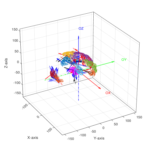
Figure 1: Overview of simulations geometry with cortex patches selected (randomly sampled during simulations) and both thalami meshes. Nodes of these meshes are candidates for source position random sampling. Red, blue and green vectors indicate SA, BN and IN respectively.

IX-D Signal in Sensor Space

The solution to forward problem (FP) is based on 1) geometry and conductivity of head compartments and 2) position of electrodes on the scalp. Based on this solution, we obtain sensor space time series y using leadfields calculated for each bioelectrical activity source defined by its position and orientation and applying them to corresponding signal time series SA, IN, BN in source space, with added MN signal, cf. models (1) and (10). We note that for large power of IN, model (10) realistically represents signal y, while the lower the power of IN, the more adequate model (1) becomes. We will observe implications of this fact below, when discussing performance results of filters under consideration.

IX-E Simulations Settings and Configuration

Simulations framework provided with the current paper enables to freely change essential simulation parameters. These include:

• signal to interference noise ratio (SINR) defined as the power of IN signal projected onto sensor space to the power of SA signal projected onto sensor space,

• signal to biological noise ratio (SBNR) defined as the power of BN signal projected onto sensor space to the power of SA signal projected onto sensor space,

• signal to measurement noise ratio (SMNR) defined as the power of MN signal to the power of SA signal projected onto sensor space,

• the number of cortical ROIs to be randomly selected,

• the number of sources (of each type, per any of the cortical and subcortical regions described above). For the results presented in Figs.2-3, we selected $l=13$ sources of interest, $k=27$ sources of interfering activity, $p=27$ sources of background activity ($7$ on the cortex, and remaining $20$ in subcortical regions),

• the number of simulation runs where new MVAR model is generated in each run,

• the number of independent realizations based on each generated MVAR model (trials).

• the number of time samples per trial,

• order of the MVAR model used to generate time-courses for signal of interest,

• presence or absence of the evoked (phase locked) activity in the source space time series.

The specific parameter values used to obtain simulation results described herein are presented jointly with results on Figs.2-3. Furthermore, in order to model mislocalization of sources, we used perturbed leadfields for the source activity reconstruction. Namely, we shifted position of leadfields randomly by $<5$ mm in each direction $(x,y,z)$ and its orientation is rotated by $<\frac{\pi}{32}$ (azimuth and elevation). We considered patch-constraints, where the rank $s$ of the approximation $H_{I_{s}}$ of forward matrix $H_{I}$ of interfering sources was set to $8$, to keep approximately $30\%$ of singular values of $H_{I}.$ These parameters are also adjustable in the proposed framework.

For each combination of SNRs we conducted 100 simulation runs. In each run, locations for bioelectrical sources of activity were randomly chosen in accordance to the above mentioned scheme and a new MVAR model was generated.

Each simulation run contained 100 realizations of the MVAR process that constituted 100 trials and each trial consisted of 1000 signal samples, where:

• The first half (i.e., the first 500 samples) of each trial is interpreted as pre-task/stimulus activity and is comprised of BN signal projected onto sensor space along with MN signal. The estimate of noise covariance matrix $N$ is obtained from this signal as a finite sample estimate.

• The second half of each trial is comprised of all signals, i.e., SA, IN, BN signals projected onto sensor space along with MN signal. The estimate of signal covariance matrix $R$ is obtained from this signal as a finite sample estimate.

IX-F Performance Evaluation

To facilitate fair comparison of performance of proposed filters, we selected for evaluation the following range of widely used spatial filters:

• The LCMV filter, expressed as both

  $$W_{LCMV(R)}=(H^{t}R^{-1}H)^{-1}H^{t}R^{-1}$$

  and

  $$W_{LCMV(N)}=(H^{t}N^{-1}H)^{-1}H^{t}N^{-1},$$

  cf. Remark 1.

• The nulling filter in the form proposed in the work [25], namely

  $$W_{NL}=[I_{l}\ 0_{l\times k}](H_{c}^{t}R^{-1}H_{c})^{-1}H_{c}^{t}R^{-1},$$

  cf. (13).

• The eigenspace-LCMV filters [5] exploiting projection of the signal covariance matrix onto its principal subspace of the forms

  $$W_{EIG-LCMV(R)}=W_{LCMV(R)}P_{R_{sig}},$$

  where $P_{R_{sig}}$ is the orthogonal projection matrix onto subspace spanned by eigenvectors corresponding to $\lambda_{1}\geq\dots\geq\lambda_{sig}$ - the $sig$ largest eigenvalues of $R$, where $sig$ is the dimension of signal subspace. In practice, it is difficult to estimate signal subspace dimension [5]. Here, we selected $sig$ to match the number of active sources assumed, i.e., the optimal value of $sig.$

• The theoretically MSE-optimal MMSE (Wiener) filter for the interference-free case, defined as $W_{MMSE}=QHR^{-1}.$

• The zero-forcing filter, defined as $W_{ZF}=H^{\dagger}.$

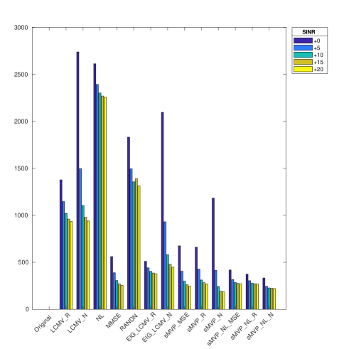
Figure 2: Spatial filters performance: cumulative error measured as Euclidean distance between the original and reconstructed time series for: SMNR=10, SBNR=0 and SINR=0,5,10,15 and 20 dB.

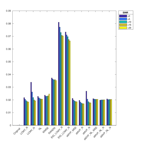
Figure 3: Spatial filters performance: cumulative error measured as Euclidean distance between the original and reconstructed PDC values for: SMNR=10, SBNR=0 and SINR=0,5,10,15 and 20 dB.

Additionally, as a sanity-check, we also considered random and zero filters, defined as random (with standard normal-Gaussian- entries) and zero matrices of suitable sizes, respectively. However, the zero-forcing, random and zero filters are not presented in Figs.2-3, as they achieve too large error to scale with other filters considered.

From Fig.2, it is seen that for lower values of SINR, the nulling filters achieve advantage over filters designed for interference-free model, which is incorrect in such settings. On the other hand, for high values of SINR, the interference-free model better reflects observed signal, and filters designed for this model achieve comparable or better performance than their counterparts derived for the model in presence of interference. Moreover, Fig.3 demonstrates that MSE-fidelity in reconstruction performance is correlated with degree of accuracy of PDC values based on reconstructed activity of the sources, but there is no direct linkage between them. Indeed, the eigenspace-LCMV filters produce reconstruction particularly ill-suited to this aim. We emphasize that the presented figures are for illustrative purpose and we invite readers to test other settings.

IX-G Event-Related Experiments

In the simulation framework proposed in this section we did not insist on a specific type of EEG/MEG measurements. In particular, the proposed framework is applicable to all types of EEG/MEG measurements, including event-related EEG/MEG experiments, where one may be interested in reconstructing activity which is evoked (phase-locked) or induced (non-phase locked) to the stimulus. In such experiments, we usually have stationarity in the covariance, but not in the mean [6], due to presence of both evoked and induced part of the brain response to the stimuli [41]. Then, if one is interested in reconstruction of evoked (phase-locked) response, we recommend to use the filter minimizing directly the power of reconstructed noise, i.e., filter of the form (26) if presence of interference is assumed, or of the form (54) if the interference-free model is assumed. On the other hand, if one is interested in reconstruction of induced (non-phase-locked) response, one may simply subtract the phase-locked activity beforehand, see, e.g., [25].

X Conclusion

We proposed two families of novel spatial filters parameterized by filter rank. We provided a method to select this parameter minimizing MSE of the filter output. We also developed open source simulation framework for evaluation of efficiency of spatial filters which is available online. In its current form, this extensible framework enables also investigation of directed connectivity among sources of interest by means of PDC measure. We hope the proposed filters may found use within the EEG/MEG community and possibly beyond, e.g., in wireless communications.

Appendix A Known Results Used

For convenience, let us recall that in this paper we assume that all eigen- and singular value decompositions considered have their eigen- and singular values organized in nonincreasing order.

Fact 1 (Eckart-Young-Schmidt-Mirsky Theorem [42])

Let $A\in\mathbb{R}^{m\times n}$ be a given matrix of $rk(A)=a$ and let us set rank constraint $r<a.$ Then, one has:

$$X_{r}^{S}\in\bigcap_{\iota\in\mathfrak{I}}\left\{\arg\min_{X_{r}\in\mathcal{X}_{r}^{m\times n}}\parallel X_{r}-A\parallel_{\iota}\right\},$$ (60)

if $X_{r}^{S}$ is of the following form:

$$X_{r}=[U_{A}]_{m\times r}[\Sigma_{A}]_{r\times r}([V_{A}]_{n\times r})^{t},$$ (61)

where $A=U_{A}\Sigma_{A}V_{A}^{t}$ is a singular value decomposition of $A.$ Further, $X_{r}^{S}$ is a minimizer if and only if it is obtained in this way.

Fact 2 ([43, p.113])

Let $A\in\mathbb{R}^{m\times n}$ be a given matrix and let the subspace $S\subset\mathbb{R}^{n}$ be given. Then, for any $b\in\mathbb{R}^{m}$, $Xb$ is the minimum-norm least-squares solution of $Ax=b$, where $x\in S$, if and only if $X=P_{s}(AP_{s})^{\dagger}$, where $P_{s}$ is the orthogonal projection matrix onto $S.$

Fact 3 ([44])

Let $C\in\mathbb{R}^{n\times n},D\in\mathbb{R}^{n\times n}$ be symmetric matrices. Denoting by $c_{1}\geq c_{2}\geq\dots\geq c_{n}$ and $d_{1}\geq d_{2}\geq\dots\geq d_{n}$, one has

$$tr(CD)\leq\sum_{i=1}^{n}c_{i}d_{i}.$$ (62)

The equality can be attained.

Remark 11

With notation as in Fact A-3, we have equivalently:

$$tr\big{(}C(-D)\big{)}=-tr(CD)\geq-\sum_{i=1}^{n}c_{i}d_{i}.$$ (63)

Appendix B Proof of Theorem 1

Change of variables

Let us first consider $G:=R^{-1/2}H$ and $G_{I}:=R^{-1/2}H_{I}$ along with $G_{c}:=[G\ G_{I}]$ and $Z_{r}:=W_{r}R^{1/2}.$ We note that $Z_{r}G=W_{r}H$ and $Z_{r}G_{I}=W_{r}H_{I}$ and consequently $Z_{r}G_{c}=[Z_{r}G\ Z_{r}G_{I}]=[W_{r}H\ W_{r}H_{I}]=W_{r}H_{c}.$ We also note that $rk(G)=l$, $rk(G_{I})=k$, $rk(G_{c})=l+k$ and $Z_{r}\in\mathcal{X}_{r}^{{l}\times{m}}$, as multiplication by invertible matrix does not change rank of matrix [30]. Therefore, the optimization problem (17) can be recast in view of (11) and (16) in terms of these new variables equivalently as:

$$\left\{\begin{array}[]{ll}\textrm{minimize}&\parallel Z_{r}\parallel_{F}^{2}-2tr\big{(}Z_{r}G_{c}\mathbb{E}[{\textbf{q}_{c}\textbf{q}^{t}}]\big{)}\\ \textrm{subject to}&\left\{\begin{array}[]{l}Z_{r}\in\displaystyle{\bigcap_{\iota\in\mathfrak{I}}}\arg\displaystyle{\min_{Z_{r}\in\mathcal{X}_{r}^{{l}\times{m}}}}\parallel Z_{r}G-I_{l}\parallel_{\iota}^{2}\\ Z_{r}G_{I}=0_{l\times k}.\\ \end{array}\right.\\ \end{array}\right.$$ (64)

In particular, we note that the constraint $Z_{r}G_{I}=0_{l\times k}$ implies that

$$Z_{r}G_{c}\mathbb{E}[{\textbf{q}_{c}\textbf{q}^{t}}]=Z_{r}[G\ G_{I}]\mathbb{E}[{\textbf{q}_{c}\textbf{q}^{t}}]=\\ [Z_{r}G\ 0_{l\times k}]\mathbb{E}[{\textbf{q}_{c}\textbf{q}^{t}}]=Z_{r}GQ,$$ (65)

which will be useful later on, with $Q=\mathbb{E}[{\textbf{q}\textbf{q}^{t}}].$

Feasible set

In this part we reformulate the definition of feasible set of $Z_{r}$ satisfying constraints of optimization problem (64). Regarding the first constraint, we note that from Fact 1 given in the Appendix A one has that

$$\bigcap_{\iota\in\mathfrak{I}}\left\{\arg\min_{X_{r}\in\mathcal{X}_{r}^{{l}\times{l}}}\parallel X_{r}-I_{l}\parallel_{\iota}\right\}=\Lambda_{r}\Lambda_{r}^{t},$$ (66)

where $\Lambda_{r}=[\Lambda]_{l\times r}$ for an orthogonal matrix $\Lambda\in\mathbb{R}^{l\times l}.$ We further note that equation $Z_{r}G=\Lambda_{r}\Lambda_{r}^{t}$ is solvable with respect to $Z_{r}$, since, e.g., $\Lambda_{r}\Lambda_{r}^{t}G^{\dagger}$ is a particular solution. Thus, $Z_{r}$ satisfies $Z_{r}\in\displaystyle{\bigcap_{\iota\in\mathfrak{I}}}\arg\displaystyle{\min_{Z_{r}\in\mathcal{X}_{r}^{{l}\times{m}}}}\parallel Z_{r}G-I_{l}\parallel_{\iota}^{2}$ if and only if $Z_{r}G=\Lambda_{r}\Lambda_{r}^{t}$ for certain $\Lambda_{r}\in\mathbb{R}^{l\times r}$ satisfying $\Lambda_{r}^{t}\Lambda_{r}=I_{r}.$ Moreover, denoting $z^{t}_{r_{i}}$ to be the $i$-th column of $Z_{r}^{t}$ for $i=1,\dots,l$, and upon noticing that the second constraint $Z_{r}G_{I}=0_{l\times k}$ is equivalent to $z^{t}_{r_{i}}\in\mathcal{N}(G_{I}^{t})=\mathcal{R}(G_{I})^{\perp}\subset\mathbb{R}^{m}$ for $i=1,\dots,l$, it is seen that the constraints in (64) can be equivalently cast as

$$\left\{\begin{array}[]{l}Z_{r}G=\Lambda_{r}\Lambda_{r}^{t}\\ z^{t}_{r_{i}}\in\mathcal{R}(G_{I})^{\perp},i=1,\dots,l.\\ \end{array}\right.\\$$ (67)

In particular, from (65) we obtain that it is sufficient to consider only minimum-norm solutions of (67), as the cost function in (64) is in view of (65) such that

$$\parallel Z_{r}^{\star}\parallel_{F}^{2}-2tr\big{(}Z_{r}^{\star}GQ\big{)}=\\ \parallel Z_{r}^{\star}\parallel_{F}^{2}-2tr\big{(}\Lambda_{r}\Lambda_{r}^{t}Q\big{)}\leq\\ \parallel Z_{r}^{\diamond}\parallel_{F}^{2}-2tr\big{(}\Lambda_{r}\Lambda_{r}^{t}Q\big{)},$$ (68)

where $Z_{r}^{\star}$ is the minimum-norm solution of $Z_{r}G=\Lambda_{r}\Lambda_{r}^{t}$ and $Z_{r}^{\diamond}$ is any other solution of $Z_{r}G=\Lambda_{r}\Lambda_{r}^{t}$, both subject to the constraints in (67).

Minimum-norm solution

We use now Fact 2 in the Appendix A and obtain that, after transposition,

$$Z_{r}^{\star}=\Lambda_{r}\Lambda_{r}^{t}(P_{\mathcal{R}(G_{I})^{\perp}}G)^{\dagger}P_{\mathcal{R}(G_{I})^{\perp}}$$ (69)

is the least-squares solution of (67) such that $\parallel Z_{r}^{\star}\parallel_{F}^{2}$ is the smallest among all least-squares solutions of (67). We proceed now to show that $Z_{r}^{\star}$ is the minimum-norm solution of (67). To this end, we note first that the second constraint in (67) is satisfied by rows of $Z_{r}^{\star}$ (columns of $(Z_{r}^{\star})^{t}$). Thus, it suffices to show that $(P_{\mathcal{R}(G_{I})^{\perp}}G)$ is of full-column rank $l$, which will ensure that $Z_{r}^{\star}G=\Lambda_{r}\Lambda_{r}^{t}$, as in such a case $(P_{\mathcal{R}(G_{I})^{\perp}}G)^{\dagger}(P_{\mathcal{R}(G_{I})^{\perp}}G)=I_{l}$ [30].

To this end, we note that due to linear independence of columns of $G_{c}=[G\ G_{I}]$, one has in particular that $\mathcal{R}(G)\cap\mathcal{R}(G_{I})=\{0\}.$ Based on this fact, we will prove now that

$$\textrm{if }x\in\mathcal{R}(G)\textrm{ then }P_{\mathcal{R}(G_{I})^{\perp}}x=0\iff\ x=0.$$ (70)

$(\Rightarrow)$ Let us express $x\in\mathcal{R}(G)$ as $x=P_{\mathcal{R}(G_{I})}x+P_{\mathcal{R}(G_{I})^{\perp}}x.$ Then, by our assumption one has $x=P_{\mathcal{R}(G_{I})}x$, hence $x\in\mathcal{R}(G_{I}).$ Thus, $x\in\mathcal{R}(G)\cap\mathcal{R}(G_{I})$ and from the fact that $\mathcal{R}(G)\cap\mathcal{R}(G_{I})=\{0\}$ we conclude that it must be $x=0.$
$(\Leftarrow)$ This is obvious.

Based on (70), it is easy to prove that $P_{\mathcal{R}(G_{I})^{\perp}}$ is injective on $\mathcal{R}(G)$ as follows: suppose that $x_{1}\in\mathcal{R}(G),x_{2}\in\mathcal{R}(G)$, $x_{1}\neq x_{2}$, and that $P_{\mathcal{R}(G_{I})^{\perp}}x_{1}=P_{\mathcal{R}(G_{I})^{\perp}}x_{2}.$ Thus, $P_{\mathcal{R}(G_{I})^{\perp}}(x_{1}-x_{2})=0$, hence from (70) it must be $x_{1}=x_{2}$, which contradicts our assumption $x_{1}\neq x_{2}.$

Consider now the linearly independent set $\{g_{1},g_{2},\dots,g_{l}\}$ of columns of $G.$ Since $P_{\mathcal{R}(G_{I})^{\perp}}$ is injective on $\mathcal{R}(G)$, the set $\{P_{\mathcal{R}(G_{I})^{\perp}}g_{1},P_{\mathcal{R}(G_{I})^{\perp}}g_{2},\dots,P_{\mathcal{R}(G_{I})^{\perp}}g_{l}\}$ of columns of $(P_{\mathcal{R}(G_{I})^{\perp}}G)$ is also linearly independent. This implies that $rk(P_{\mathcal{R}(G_{I})^{\perp}}G)=l$, and consequently, that $(P_{\mathcal{R}(G_{I})^{\perp}}G)^{\dagger}(P_{\mathcal{R}(G_{I})^{\perp}}G)=I_{l}.$ Thus, $Z_{r}^{\star}$ in (69) is the (minimum-norm) solution of $Z_{r}G=\Lambda_{r}\Lambda_{r}^{t}$ such that $z^{t}_{r_{i}}\in\mathcal{R}(G_{I})^{\perp}$ for $i=1,\dots,l.$

Selection of subspace

It follows from the above considerations that we have narrowed the set of possible solutions of the optimization problem (64) to matrices of the form (69), parameterized by

$$P_{r}:=\Lambda_{r}\Lambda_{r}^{t},$$ (71)

which we recognize as an orthogonal projection matrix onto arbitrary subspace of $\mathbb{R}^{l}$ of dimension $r.$ Therefore, we need to determine now the form of $P_{r}$ minimizing the cost function in (64). Taking into account (65) and using the fact that $P_{r}$ and $P_{\mathcal{R}(G_{I})^{\perp}}$ are both symmetric and idempotent [30], insertion of (69) into cost function in (64) reveals

$$\parallel Z_{r}^{\star}\parallel_{F}^{2}-2tr\big{(}Z_{r}^{\star}GQ\big{)}=\\ tr\Big{(}P_{r}(P_{\mathcal{R}(G_{I})^{\perp}}G)^{\dagger}P_{\mathcal{R}(G_{I})^{\perp}}\times\\ \big{(}P_{r}(P_{\mathcal{R}(G_{I})^{\perp}}G)^{\dagger}P_{\mathcal{R}(G_{I})^{\perp}}\big{)}^{t}\Big{)}-2tr(P_{r}Q)=\\ tr(P_{r}K^{(1)}),$$ (72)

where

$$K^{(1)}=(P_{\mathcal{R}(G_{I})^{\perp}}G)^{\dagger}P_{\mathcal{R}(G_{I})^{\perp}}\big{(}(P_{\mathcal{R}(G_{I})^{\perp}}G)^{\dagger}\big{)}^{t}-2Q.$$ (73)

Clearly, $K^{(1)}$ is a symmetric matrix, and so is $P_{r}.$ Thus, by applying Fact 3 in the Appendix A along with Remark 11 we obtain, upon setting $C=P_{r}$ and $D=-K^{(1)}$ therein that $tr(P_{r}K^{(1)})$ is minimized for $P_{r}=P_{K_{r}^{(1)}}:=\Lambda_{K_{r}^{(1)}}\Lambda_{K_{r}^{(1)}}^{t}$, where $\Lambda_{K_{r}^{(1)}}\in\mathbb{R}^{l\times r}$ contains as its columns the eigenvectors corresponding to $\delta_{1}^{(1)}\leq\dots\leq\delta_{r}^{(1)}$ - the $r$ smallest eigenvalues of $K^{(1)}.$ Then, the form of solution in (20) is obtained by inverting the change of variables to $W_{r}^{\star}=Z_{r}^{\star}R^{-1/2}$, where $Z_{r}^{\star}=P_{K_{r}^{(1)}}(P_{\mathcal{R}(G_{I})^{\perp}}G)^{\dagger}P_{\mathcal{R}(G_{I})^{\perp}}.$ Moreover, from (11), (64), (65) and (72) one has

$$\mathrm{J}_{I}(W_{r}^{\star})=\parallel Z_{r}^{\star}\parallel_{F}^{2}-2tr\big{(}Z_{r}^{\star}G_{c}\mathbb{E}[{\textbf{q}_{c}\textbf{q}^{t}}]\big{)}+c=\\ tr(P_{K_{r}^{(1)}}K^{(1)})+c=\sum_{i=1}^{r}\delta_{i}^{(1)}+c,$$ (74)

where $c=tr(\mathbb{E}[{\textbf{q}\textbf{q}^{t}}])=tr(Q).$

Appendix C Proof of Theorem 2

The proof proceeds analogously to the proof of Theorem 1 above, where in place of optimization problem (64) we consider now, in view of (18):

$$\left\{\begin{array}[]{ll}\textrm{minimize}&\parallel Z_{r}\parallel_{F}^{2}\\ \textrm{subject to}&\left\{\begin{array}[]{l}Z_{r}\in\displaystyle{\bigcap_{\iota\in\mathfrak{I}}}\arg\displaystyle{\min_{Z_{r}\in\mathcal{X}_{r}^{{l}\times{m}}}}\parallel Z_{r}G-I_{l}\parallel_{\iota}^{2}\\ Z_{r}G_{I}=0_{l\times k}.\\ \end{array}\right.\\ \end{array}\right.$$ (75)

Then, in place of (72) one obtains for $Z_{r}^{\star}$ of the form (69) with $P_{r}:=\Lambda_{r}\Lambda_{r}^{t}$ as in (71) that

$$\parallel Z_{r}^{\star}\parallel_{F}^{2}=\\ tr\Big{(}P_{r}(P_{\mathcal{R}(G_{I})^{\perp}}G)^{\dagger}P_{\mathcal{R}(G_{I})^{\perp}}\big{(}P_{r}(P_{\mathcal{R}(G_{I})^{\perp}}G)^{\dagger}P_{\mathcal{R}(G_{I})^{\perp}}\big{)}^{t}\Big{)}=\\ tr(P_{r}K^{(2)}),$$ (76)

where

$$K^{(2)}=(P_{\mathcal{R}(G_{I})^{\perp}}G)^{\dagger}P_{\mathcal{R}(G_{I})^{\perp}}\big{(}(P_{\mathcal{R}(G_{I})^{\perp}}G)^{\dagger}\big{)}^{t}=K^{(1)}+2Q.$$ (77)

Clearly, $K^{(2)}$ is a symmetric matrix. Thus, in order to find the form of $P_{r}$ minimizing $tr(P_{r}K^{(2)})$, we apply Fact 3 in the Appendix A along with Remark 11 in exactly the same way as was done below (73) in the proof of Theorem 1, to obtain $P_{r}=P_{K_{r}^{(2)}}:=\Lambda_{K_{r}^{(2)}}\Lambda_{K_{r}^{(2)}}^{t}$, where $\Lambda_{K_{r}^{(2)}}\in\mathbb{R}^{l\times r}$ contains as its columns the eigenvectors corresponding to $\delta_{1}^{(2)}\leq\dots\leq\delta_{r}^{(2)}$ - the $r$ smallest eigenvalues of $K^{(2)}.$ Similarly as above, the form of solution in (23) is obtained by inverting the change of variables to $W_{r}^{\star}=Z_{r}^{\star}R^{-1/2}$, where $Z_{r}^{\star}=P_{K_{r}^{(2)}}(P_{\mathcal{R}(G_{I})^{\perp}}G)^{\dagger}P_{\mathcal{R}(G_{I})^{\perp}}.$ Moreover, just as in (74) above, we obtain

$$\mathrm{J}_{I}(W_{r}^{\star})=\parallel Z_{r}^{\star}\parallel_{F}^{2}-2tr\big{(}Z_{r}^{\star}G_{c}\mathbb{E}[{\textbf{q}_{c}\textbf{q}^{t}}]\big{)}+c=\\ tr(P_{K_{r}^{(2)}}K^{(1)})+c=tr\big{(}P_{K_{r}^{(2)}}(K^{(2)}-2Q)\big{)}+c=\\ \sum_{i=1}^{r}\delta_{i}^{(2)}-2tr(P_{K_{r}^{(2)}}Q)+c,$$ (78)

where $c=tr(\mathbb{E}[{\textbf{q}\textbf{q}^{t}}])=tr(Q).$

Appendix D Proof of Theorem 3

The closed algebraic form (26) of the solution of the optimization problem (19) is obtained in exactly the same way as in the proof of Theorem 2, with $G$ replaced by $F$, $G_{I}$ replaced by $F_{I}$, and $G_{c}$ replaced by $F_{c}$, respectively. Thus, to complete the proof of Theorem 3 we only need to compute $\mathrm{J}_{I}(W_{r}^{\star})$, where $W_{r}^{\star}=Z_{r}^{\star}N^{-1/2}$ with $Z_{r}^{\star}=P_{K_{r}^{(3)}}\big{(}P_{\mathcal{R}(F_{I})^{\perp}}F\big{)}^{\dagger}P_{\mathcal{R}(F_{I})^{\perp}}.$ Namely, using (65) for $F$ and $F_{I}$, we have:

$$\mathrm{J}_{I}(W_{r}^{\star})=tr(W_{r}^{\star}R(W_{r}^{\star})^{t})-2tr\big{(}W_{r}^{\star}H_{c}\mathbb{E}[{\textbf{q}_{c}\textbf{q}^{t}}]\big{)}+c=\\ tr(W_{r}^{\star}\underbrace{(H_{c}Q_{c}H_{c}^{t}+N)}_{R}(W_{r}^{\star})^{t})-2tr\big{(}W_{r}^{\star}H_{c}\mathbb{E}[{\textbf{q}_{c}\textbf{q}^{t}}]\big{)}+c=\\ tr(Z_{r}^{\star}F_{c}Q_{c}F_{c}^{t}(Z_{r}^{\star})^{t})+tr(Z_{r}^{\star}(Z_{r}^{\star})^{t})-2tr\big{(}Z_{r}^{\star}F_{c}\mathbb{E}[{\textbf{q}_{c}\textbf{q}^{t}}]\big{)}+c=\\ tr(Z_{r}^{\star}FQF^{t}(Z_{r}^{\star})^{t})+tr(Z_{r}^{\star}(Z_{r}^{\star})^{t})-2tr\big{(}Z_{r}^{\star}FQ\big{)}+c=\\ tr\big{(}P_{K_{r}^{(3)}}Q(P_{K_{r}^{(3)}})^{t}\big{)}+\parallel Z_{r}^{\star}\parallel_{F}^{2}-2tr\big{(}P_{K_{r}^{(3)}}Q\big{)}+c=\\ \parallel Z_{r}^{\star}\parallel_{F}^{2}-tr(P_{K_{r}^{(3)}}Q)+c=\\ tr(P_{K_{r}^{(3)}}K^{(4)})+c,$$ (79)

where $c=tr(\mathbb{E}[{\textbf{q}\textbf{q}^{t}}])=tr(Q)$ and

$$K^{(4)}=(P_{\mathcal{R}(F_{I})^{\perp}}F)^{\dagger}P_{\mathcal{R}(F_{I})^{\perp}}\big{(}(P_{\mathcal{R}(F_{I})^{\perp}}F)^{\dagger}\big{)}^{t}-Q=\\ K^{(3)}-Q.$$ (80)

Finally,

$$\mathrm{J}_{I}(W_{r}^{\star})=tr\big{(}P_{K_{r}^{(3)}}(K^{(3)}-Q)\big{)}+c=\\ \sum_{i=1}^{r}\delta_{i}^{(3)}-tr(P_{K_{r}^{(3)}}Q)+c.\$$ (81)

References

• [1] O. L. Frost, “An algorithm for linearly constrained adaptive array processing,” Proc. IEEE, vol. 60, no. 8, pp. 926–935, 1972.
• [2] B. D. Van Veen, W. Van Drongelen, M. Yuchtman, and A. Suzuki, “Localization of brain electrical activity via linearly constrained minimum variance spatial filtering,” IEEE Trans. Biomed. Eng., vol. 44, no. 9, pp. 867–880, Sep. 1997.
• [3] J. Gross, J. Kujala, M. Hämäläinen, L. Timmermann, A. Schnitzler, and R. Salmelin, “Dynamic imaging of coherent sources: Studying neural interactions in the human brain,” Proceedings of the National Academy of Sciences, vol. 98, no. 2, pp. 694–699, 2001.
• [4] K. Sekihara, S. S. Nagarajan, D. Poeppel, A. Marantz, and Y. Miyashita, “Reconstructing spatio-temporal activities of neural sources using an MEG vector beamformer technique,” IEEE Trans. Biomed. Eng., vol. 48, no. 7, pp. 760–771, 2001.
• [5] K. Sekihara and S. S. Nagarajan, Adaptive Spatial Filters for Electromagnetic Brain Imaging.   Berlin: Springer, 2008.
• [6] A. Moiseev, J. M. Gaspar, J. A. Schneider, and A. T. Herdman, “Application of multi-source minimum variance beamformers for reconstruction of correlated neural activity,” NeuroImage, vol. 58, no. 2, pp. 481–496, Sep. 2011.
• [7] M. Diwakar, M.-X. Huang, R. Srinivasan, D. L. Harrington, A. Robb, A. Angeles, L. Muzzatti, R. Pakdaman, T. Song, R. J. Theilmann, and R. R. Lee, “Dual-core beamformer for obtaining highly correlated neuronal networks in MEG,” NeuroImage, vol. 54, no. 1, pp. 253–263, Jan. 2011.
• [8] R. Oostenveld, P. Fries, E. Maris, and J.-M. Schoffelen, “FieldTrip: Open source software for advanced analysis of MEG, EEG, and invasive electrophysiological data,” Computational Intelligence and Neuroscience, no. 156869, 2011.
• [9] F. Tadel, S. Baillet, J. Mosher, D. Pantazis, and R. M. Leahy, “Brainstorm: A user-friendly application for MEG/EEG analysis,” Computational Intelligence and Neuroscience, no. 879716, 2011.
• [10] A. Gramfort, M. Luessi, E. Larson, D. Engemann, D. Strohmeier, C. Brodbeck, L. Parkkonen, and M. Hämäläinen, “MNE software for processing MEG and EEG data,” NeuroImage, vol. 86, pp. 446–460, 2014.
• [11] A. Keitel and J. Gross, “Individual human brain areas can be identified from their characteristic spectral activation fingerprints,” PLoS Biol., vol. 14, no. 6, p. e1002498, 2016.
• [12] M. Siems, A.-A. Pape, J. F. Hipp, and M. Siegel, “Measuring the cortical correlation structure of spontaneous oscillatory activity with EEG and MEG,” NeuroImage, vol. 129, pp. 345–355, 2016.
• [13] I. Yamada and J. Elbadraoui, “Minimum-variance pseudo-unbiased low-rank estimator for ill-conditioned inverse problems,” in Proc. ICASSP, Toulouse, France, May 2006, pp. 325–328.
• [14] T. Piotrowski and I. Yamada, “MV-PURE estimator: Minimum-variance pseudo-unbiased reduced-rank estimator for linearly constrained ill-conditioned inverse problems,” IEEE Trans. Signal Process., vol. 56, no. 8, pp. 3408–3423, Aug. 2008.
• [15] T. Piotrowski, R. L. G. Cavalcante, and I. Yamada, “Stochastic MV-PURE estimator: Robust reduced-rank estimator for stochastic linear model,” IEEE Trans. Signal Process., vol. 57, no. 4, pp. 1293–1303, Apr. 2009.
• [16] M. Yamagishi and I. Yamada, “A rank selection of MV-PURE with an unbiased predicted-MSE criterion and its efficient implementation in image restoration,” in Proc. IEEE ICASSP, Vancouver, Canada, May 2013, May 2013, pp. 1573–1577.
• [17] T. Piotrowski and I. Yamada, “Performance of the stochastic MV-PURE estimator in highly noisy settings,” J. of The Franklin Institute, vol. 351, no. 6, pp. 3339–3350, Jun. 2014.
• [18] D. R. Brillinger, Time Series: Data Analysis and Theory.   New York: Holt, Rinehart and Winston, 1975.
• [19] L. L. Scharf, “The SVD and reduced rank signal processing,” Signal Process., vol. 25, pp. 113–133, 1991.
• [20] P. Stoica and M. Viberg, “Maximum likelihood parameter and rank estimation in reduced-rank multivariate linear regressions,” IEEE Trans. Signal Process., vol. 44, no. 12, pp. 3069–3078, Dec. 1996.
• [21] Y. Yamashita and H. Ogawa, “Relative Karhunen-Loeve transform,” IEEE Trans. Signal Process., vol. 44, no. 2, pp. 371–378, Feb. 1996.
• [22] L. L. Scharf and J. K. Thomas, “Wiener filters in canonical coordinates for transform coding, filtering, and quantizing,” IEEE Trans. Signal Processing, vol. 46, pp. 647–654, Mar. 1998.
• [23] T. Piotrowski and I. Yamada, “Reduced-rank estimation for ill-conditioned stochastic linear model with high signal-to-noise ratio,” J. of The Franklin Institute, vol. 353, no. 13, pp. 2898–2928, Sep. 2016.
• [24] S. S. Dalal, K. Sekihara, and S. S. Nagarajan, “Modified beamformers for coherent source region suppression,” IEEE Trans. Biomed. Eng., vol. 53, no. 7, pp. 1357–1363, Jul. 2006.
• [25] H. B. Hui, D. Pantazis, S. L. Bressler, and R. M. Leahy, “Identifying true cortical interactions in MEG using the nulling beamformer,” NeuroImage, vol. 49, no. 4, pp. 3161–3174, 2010.
• [26] L. A. Baccala and K. Sameshima, “Partial directed coherence: a new concept in neural structure determination,” Biol. Cybern., vol. 84, no. 6, pp. 463–474, 2001.
• [27] R. Kuś, M. Kamiński, and K. Blinowska, “Determination of eeg activity propagation: pair-wise versus multichannel estimate,” IEEE Trans. Biomed. Eng., vol. 51, no. 9, pp. 1501–1510, 2004.
• [28] T. Piotrowski, C. Zaragoza-Martinez, D. Gutierrez, and I. Yamada, “MV-PURE estimator of dipole source signals in EEG,” in Proc. ICASSP, Vancouver, Canada, May 2013, May 2013, pp. 968–972.
• [29] T. Piotrowski, J. Nikadon, and D. Gutierrez, “Reconstruction of brain activity in EEG/MEG using reduced-rank nulling spatial filter,” in Proc. SSP, Palma de Mallorca, Spain, June 2016, Jun. 2016, pp. 1–5.
• [30] R. A. Horn and C. R. Johnson, Matrix Analysis.   New York: Cambridge University Press, 1985.
• [31] R. D. Pascual-Marqui, “Review of methods for solving the EEG inverse problem,” International Journal of Bioelectromagnetism, vol. 1, no. 1, pp. 75–86, 1999.
• [32] T. Piotrowski, D. Gutierrez, I. Yamada, and J. Zygierewicz, “Reduced-rank neural activity index for EEG/MEG multi-source localization,” in Proc. IEEE ICASSP, Florence, Italy, May 2014, pp. 4708–4712.
• [33] ——, “A family of reduced-rank neural activity indices for EEG/MEG source localization,” LNCS, vol. 8609, pp. 447–458, Aug. 2014.
• [34] J. C. Mosher, R. M. Leahy, and P. S. Lewis, “EEG and MEG: forward solutions for inverse methods,” IEEE Trans. Biomed. Eng., vol. 46, no. 3, pp. 245–259, Mar. 1999.
• [35] A. Moiseev, S. M. Doesburg, R. E. Grunau, and U. Ribary, “Minimum variance beamformer weights revisited,” NeuroImage, vol. 120, pp. 201–213, 2015.
• [36] Y. Hua, M. Nikpour, and P. Stoica, “Optimal reduced-rank estimation and filtering,” IEEE Trans. Signal Process., vol. 49, no. 3, pp. 457–469, Mar. 2001.
• [37] D. Gutiérrez, A. Nehorai, and A. Dogandžić, “Performance analysis of reduced-rank beamformers for estimating dipole source signals using EEG/MEG,” IEEE Trans. Biomed. Eng., vol. 53, no. 5, pp. 840–844, 2006.
• [38] S. Haufe, V. V. Nikulin, K.-R. Müller, and G. Nolte, “A critical assessment of connectivity measures for EEG data: A simulation study,” NeuroImage, vol. 64, pp. 120 – 133, 2013.
• [39] T. Oostendorp and A. Van Oosterom, “Source parameter estimation in inhomogeneous volume conductors of arbitrary shape,” Biomedical Engineering, IEEE Transactions on, vol. 36, no. 3, pp. 382–391, March 1989.
• [40] A. M. Dale, B. Fischl, and M. I. Sereno, “Cortical surface-based analysis: I. segmentation and surface reconstruction,” NeuroImage, vol. 9, no. 2, pp. 179–194, 1999.
• [41] O. David, J. M. Kilner, and K. J. Friston, “Mechanisms of evoked and induced responses in MEG / EEG,” NeuroImage, vol. 31, no. 4, pp. 1580–1591, 2006.
• [42] L. Mirsky, “Symmetric gauge functions and unitarily invariant norms,” The Quarterly Journal of Mathematics, vol. 11, no. 1, pp. 50–59, 1960.
• [43] A. Ben-Israel and T. N. E. Greville, Generalized Inverses : Theory and Applications, Second Edition.   New York: Springer Verlag, 2003.
• [44] C. M. Theobald, “An inequality for the trace of the product of two symmetric matrices,” Math. Proc. Camb. Phil. Soc., vol. 77, pp. 265–267, 1975.