Censored pairwise likelihood-based tests for mixing coefficient of spatial max-mixture models

Abstract

Max-mixture processes are defined as $Z=\max(aX\/,(1-a)Y)$ with $X$ an asymptotic dependent (AD) process, $Y$ an asymptotic independent (AI) process and $a\in[0\/,1]$. So that, the mixing coefficient $a$ may reveal the strength of the AD part present in the max-mixture process. In this paper we focus on two tests based on censored pairwise likelihood estimates. We compare their performance through an extensive simulation study. Monte Carlo simulation plays a fundamental tool for asymptotic variance calculations. We apply our tests to daily precipitations from the East of Australia. Drawbacks and possible developments are discussed.

Keywords: Composite likelihood, Max-stable process; Max-mixture models; Pairwise likelihood; Monte Carlo simulation.

1 Introduction

The rise of risky environmental events leads to renewed interest in the statistical modelling of extremes, for example modelling extreme precipitation is pivotal in flood protection. In the last decade, max-stable (MS) models have arised as a common tool for modeling spatial extremes, since they extend the gereralized extreme value (GEV) distribution to the spatial setting, providing a consistent multivariate distributions for maxima in arbitrary dimensions.

Max-stable (MS) processes for spatial data were first constructed using the spectral representation of [13]. Subsequent developments have been done on the construction of MS process models, [27], [26], [17], and [9].

Despite many attractive properties of MS models, these processes are restricted since only AD or exact indpendence can be modeled. This drawback is constraining when modeling the tail behavior of the multivariate distribution of the data, since it is difficult to asses in practice whether a data set should be modeling using asymptotic dependent (AD) or asymptotic independent (AI) models [28] and [10]. In [32], a flexible class of models which may take into account AD and AI is proposed. Theses models, called max-mixture (MM), are a mixture of a MS process and an AI process: $Z=\max(aX\/,(1-a)Y)$, with $X$ an AD process, $Y$ an (AI) process and $a\in[0\/,1]$. So that, $a$ represents the proportion of AD in the process $Z$ and our purpose is to propose statistical tests on the value of $a$.
 
To the best of our knowledge, only a few papers address testing AI issue for spatial extreme fields. E.g., in [1] a statistical test for AI of a bivariate maxima vector is proposed and a generalization to spatial context is done. It is based on the $F$- madogram [6].Standard likelihood inference on the parameters of MS models is not possible in general, since the full likelihood is not easily computable for MS vector in dimension greater than $2$. Composite likelihood are usefull when the fully specified likelihood is computationally cumbersome, or when a fully specified model is out of reach [21] and [29]. Maximum pairwise likelihood estimation for MS models weren first suggested by [24] and is now widely used. In particular, in [32] and [2] the parameter inference for MM processes have been driven.

In this paper, we propose a test on the mixing value $a$ of a MM process. This is achieved using pairwise likelihood statistics. The paper organised as follows. Section 2 reviews the theory of spatial extreme processes MS and MM. The censored pairwise likelihood approach is presented for the statistical inference in Section 3, our testing proposal approach and the main properties are detailed in Section 4. In Section 5 we show, by means of a series of simulation studies the performance of our proposed tests. In section 6 we illustrate our testing approach by the analysis of daily precipitation from the East of Australia. Concluding remarks and some perspectives are addressed in Section 7.

2 Spatial extremes modeling

Throughout our work, $X=\{X(s)\/,s\in\mathcal{X}\}$, $\mathcal{X}\subset\mathbb{R}^{d}$ (generally, $d=2$) is a spatial process will be assumed to be stationary and isotropic.

2.1 Max-stable processes

Let $\{X_{k}(s):s\in\mathcal{X}\subset\mathbb{R}^{d}\}$, $k=0,1,2,...,$ are independent replicates of a stochastic process $X$. Then $X$ is a MS process if and only if there exist a sequence of continuous functions $\{a_{n}(s)>0\}$ and $\{b_{n}(s)\}$ such that the rescaled process of maxima, $a^{-1}_{n}(s)\{\max(X_{1},X_{2},...,X_{n})-b_{n}(s)\}$, converges in distribution to $X(s)$ (see [12] for more details). By this definition, MS processes offer a natural choice for modeling spatial extremes.

The univariate extreme value theory, implies that the marginal distributions of $X(s)$ are Generalized Extreme value (GEV) distributed, and without loss of generality the margins can transformed to a simple MS process called standard Fréchet distribution, $\mathbb{P}(X(s)\leq z)=\exp\{-z^{-1}\}$.

Following [13] and [26], a simple MS process $X(s)$ has the following representation

$$X(s)=\max_{k\geq 1}Q_{k}(s)/P_{k},\qquad s\in\mathcal{X}.$$ (2.1)

where $Q_{k}(s)$ are independent replicates of a non-negative stochastic process $Q(s)$ with unit mean at each $s$, and $P_{k}$ are the points of a unit rate Poisson process $(0,\infty)$.

The joint distribution function of the process $X(s)$ at $K$ locations $s_{1}\/,\ldots\/,s_{K}\in\mathcal{X}$ is given by

$$\mathbb{P}(X(s_{1})\leq z_{1}\/,\ldots\/,X(s_{K})\leq z_{K})=G_{s_{1}\/,\ldots\/,s_{K}}(z_{1},...,z_{K})=\exp\{-V_{s_{1}\/,\ldots\/,s_{K}}(z_{1},...,z_{K})\}$$ (2.2)

where $V_{s_{1}\/,\ldots\/,s_{K}}(.)$ is called the exponent measure. It summarises the structure of extremal dependence and satisfies the property of homogenity of order $-1$ and $V_{s_{1}\/,\ldots\/,s_{K}}(\infty,...,z,...,\infty)=z^{-1}$. It has to be noted that

$$\mathbb{P}\{X(s_{1})\leq z,..,X(s_{K})\leq z\}=\exp\{-V_{s_{1}\/,\ldots\/,s_{K}}(1,...,1)/z\}=\exp\{-1/z\}^{\theta_{s_{1}\/,\ldots\/,s_{K}}}\/,$$

with $\theta_{s_{1}\/,\ldots\/,s_{K}}=V_{s_{1}\/,\ldots\/,s_{K}}(1,...,1)$. The coefficient $\theta_{s_{1}\/,\ldots\/,s_{K}}$ is known as the extremal coefficient. It can be seen as a summary of extremal dependence with two boundary values, complete dependence $\theta_{s_{1}\/,\ldots\/,s_{K}}=1$, and complete independence, $\theta_{s_{1}\/,\ldots\/,s_{K}}=K$. In the bivariate case, the AI and AD between a pair of random variables $Z_{1}$ and $Z_{2}$, with marginal distributions $F_{1}$ and $F_{2}$, may be identified by

$$\chi=\lim_{u\,\to\,1^{-}}P(F_{1}(Z_{1})>u|F_{2}(Z_{2})>u))\/.$$ (2.3)

The cases $\chi=0$ and $\chi>0$ represent AI and AD, respectively, [16]. This coefficient is related to the pairwise extremal coefficient $\theta$ through the relation $\chi=2-\theta$.

Since both dependence functions $\theta$ and $\chi$ are useless for AI processes, [5] proposed a new dependence coefficient which measures the strength of dependence for AI processes:

$$\bar{\chi}=\lim_{u\,\to\,1^{-}}\bar{\chi}(u)=\lim_{u\,\to\,1^{-}}\frac{2\log P(F(Z(s))>u)}{\log P(F(Z(s))>u,F(Z(s+h))>u)}-1$$ (2.4)

AD (respectively AI) is achieved if and if $\bar{\chi}=1$ (resp. $\bar{\chi}<1$).

Different choices for the process $Q(s)$ in (2.1) lead to some useful MS models, commonly used choices are the Guassian extreme value process [27], the extremal Gaussian process [26], the Brown-Resnick process [17], and the extremal t process [22]. Below, we list two specific examples of MS process models.

The storm profile model [27], is defined by taking $Q_{k}(s)=f(s-{\color[rgb]{0,0,0}P}_{k})$, where $f$ is a Guassian density with covariance matrix $\Sigma\in\mathbb{R}^{2\times 2}$, and ${\color[rgb]{0,0,0}P}_{k}$ is a homogenous Poisson process. The bivariate marginal probability distribution of the Smith model has the form

$${\color[rgb]{0,0,0}\mathbb{P}(X(s)\leq z_{1}\/,X(s+h)\leq z_{2})=G_{h}(z_{1},z_{2})}=\exp\left\{-\left[\frac{1}{z_{1}}\Phi\left(\frac{\gamma(h)}{2}+\frac{1}{\gamma(h)}\log\frac{z_{2}}{z_{1}}\right)+\right.\right.$$

$$\left.\left.\frac{1}{z_{2}}\Phi\left(\frac{\gamma(h)}{2}+\frac{1}{\gamma(h)}\log\frac{z_{1}}{z_{2}}\right)\right]\right\}$$

where $\gamma(h)=\sqrt{h^{T}\Sigma^{-1}h}$, in which $h$ is the seperation vector between the two locations,$\ s_{1}$, and $\ s_{2}$, and $\Phi$ is the standard normal distribution. The pairwise extremal coefficient is ${\color[rgb]{0,0,0}\theta_{s\/,s+h}=}\theta(h)=2\Phi\{\gamma(h)/2\}$.

The Truncated Extremal Gaussian (TEG) model is originally due to [26], it is defined using

$$Q_{k}(s)=c\max(0,\varepsilon_{k}(s))\mathbbm{1}_{\mathcal{A}_{k}}{(s-{\color[rgb]{0,0,0}P}_{k})}$$ (2.5)

where $\varepsilon_{k}(s)$ are independent replicates of a stationary Gaussian process $\varepsilon=\{\varepsilon(s),s\in\mathcal{X}\}$ with zero mean, unit variance and correlation function $\rho(.)$. $\mathbbm{1}_{\mathcal{A}}$ is the indicator function of a compact random set $\mathcal{A}\subset\mathcal{X}$, $\mathcal{A}_{k}$ are indepndent replicates of $\mathcal{A}$ and ${\color[rgb]{0,0,0}P}_{k}$ are points of Poisson process with a unit rate on $\mathcal{X}$. The constant $c$ is chosen to satisfy the constraint $\mathbb{E}\{Q_{k}(s)\}=1$.

The bivariate marginal probability distribution of TEG model in the stationary case has the form

$${\color[rgb]{0,0,0}\mathbb{P}(X(s)\leq z_{1}\/,X(s+h)\leq z_{2})=G_{h}(z_{1},z_{2})}=\exp\left\{-\left(\frac{1}{z_{1}}+\frac{1}{z_{2}}\right)\right.\cdot$$ (2.6)

$$\left.\left[1-\frac{\alpha(h)}{2}\left(1-\sqrt{1-\frac{2(\rho(h)+1)z_{1}z_{2}}{(z_{1}+z_{2})^{2}}}\right)\right]\right\}$$

where $h$ is the spatial lag, and $\alpha(h){\color[rgb]{0,0,0}=}(1-h/2r)\mathbbm{1}_{[0,2r]}$ if $\mathcal{A}$ is a disk of fixed radius $r$. The pairwise extremal coefficient $\theta(h)=2-\alpha({h})\{1-\sqrt{(1-\rho(h))/2}\}$. TEG model were fitted by [9] to extreme temperature data.

The stochastic process $X(s)$ defined in equation(2.1) has the bivariate density function

$$g(z_{1},z_{2})=\left\{\frac{\partial}{\partial z_{1}}V_{X}(z_{1},z_{2})\frac{\partial}{\partial z_{2}}V_{X}(z_{1},z_{2})-\frac{\partial^{2}}{\partial z_{1}z_{2}}V_{X}(z_{1},z_{2})\right\}\exp\{-V_{X}(z_{1},z_{2})\}$$

where $V_{X}$ is the exponent measure of the MS process $X(s)$.

2.2 Hybrid models of spatial extremal dependence

Although MS models seems to be suitable for modeling extremely high threshold exceedances, AI models may show a better fit at finite thresholds. Since it may be difficult or impossible in practice to decide whether a dataset should be modeled using AD or AI, [32] have introduced an hybrid spatial dependence model, which is able to capture both AD and AI.
Let $X(s),s\in\mathcal{X}$, be a stationary simple MS process, and $Y(s),s\in\mathcal{X}$, be a stationary AI process with unit Fréchet margins (see below for the construction of such a process). Then for a mixture proportion $\ a\in[0,1]$, a spatial max-mixture (MM) process is constructed:

$$Z(s)=\max\{\ aX(s),(1-\ a)Y(s)\}$$ (2.7)

The bivariate distribution function for a pair of sites is straightforwardly obtained by the independence between the processes $X$ and $Y$

$${\color[rgb]{0,0,0}G_{h}}(z_{1},z_{2})={\color[rgb]{0,0,0}G_{h}^{X}}\left(\frac{z_{1}}{\ a},\frac{z_{2}}{\ a}\right){\color[rgb]{0,0,0}G_{h}^{Y}}\left(\frac{z_{1}}{1-\ a},\frac{z_{2}}{1-\ a}\right)$$ (2.8)

where $G_{h}^{X}$ (resp. $G_{h}^{Y}$) is the bivariate distribution function of $X$, with space lag $h$ (resp. of $Y$).
AI processes with unit Fréchet marginal distributions can easily be constructed (see [32]). Consider $Y(s)=-1/\log(\varPhi(Y^{\prime}(s)))$, where $\{Y^{\prime}(s),s\in\mathcal{X}\}$ is a Gaussian process. Then, $Y$ is an AI process with unit Fréchet marginal distributions. Another class of AI processes called inverted max-stable (IMS) processes are defined using a simple MS process $\ X(s)$, let

$$Y(s)=-1/\log\{{1-\exp{[-X(s)^{-1}]}}\}$$ (2.9)

With this construction, any MS process may be transformed to provide an AI counterpart. Bivariate distribution function and density of the margins of $Y(s)$ are respectively

$$G_{h}^{Y}(z_{1},z_{2})=-1+\exp(-z^{-1}_{1})+\exp(-z^{-1}_{2})+\exp\{-V_{h}^{Y}{[\omega(z_{1}),\omega(z_{2})]}\}$$ (2.10)

$$g_{h}^{Y}(z_{1},z_{2}) =\left\{\frac{\partial}{\partial z_{1}}V_{h}^{Y}[\omega(z_{1}),\omega(z_{2})]\frac{\partial}{\partial z_{2}}V_{h}^{Y}[\omega(z_{1}),\omega(z_{2})]-\frac{\partial^{2}}{\partial z_{1}z_{2}}V_{h}^{Y}[\omega(z_{1}),\omega(z_{2})]\right\}$$

$$\times\exp\{-V_{h}^{Y}[\omega(z_{1}),\omega(z_{2})]\}\frac{\omega^{2}(z_{1})\omega^{2}(z_{2})\exp\{-(z_{1}^{-1}+z_{2}^{-1})\}}{z_{1}^{2}z_{1}^{2}\{1-\exp(-z_{1}^{-1}\}\{1-\exp(-z_{1}^{-1}\}}$$

where $V_{h}^{Y}$ is the exponent measure of the bivariate distribution $(Y(s),Y(s+h))$, and $\omega(z)=-1/\log\{{1-\exp{[-z^{-1}]}}\}$.
Thus, in the case where $X(s)$ is a MS process and $Y(s)$ is a IMS process, the distribution function in (2.8) has the form

$$\exp\{-aV_{X}(z_{1},z_{2})\}\{-1+\exp[-(1-a)/z_{1}]+\exp[-(1-a)/z_{2}]+\exp[-V_{Y}[\omega({1-a}/{z_{1}}),\omega(1-a/z_{2})]\}$$ (2.11)

[2] analyzed daily rainfall data in the east of Australia with a class of different models (MS, AI, and MM), and showed that MM models has the merit to overcome the limits of MS models in which only AD or exact independence can be modeled.

3 Inference for MM processes: censored pairwise likelihood approach

In order to propose a testing procedure on on the mixing coefficient a of MM processes defined by equation (2.7), we shall use the composite likelihood.

The composite likelihood technique [21] is a general method of inference for dealing with large datasets and/or miss-specified models. A composite likelihood consists of a combination of valid likelihood objects usually related to small subsets of data and defined as

$$\mathcal{L}_{C}=\prod_{k=1}^{K}g(z\in\mathcal{B}_{k};\varphi)^{\omega_{k}}$$ (3.1)

where $\{g(z\in\mathcal{B}_{k};\varphi),z\in\mathcal{Z}\subseteq\mathbb{R}^{K},\varphi\in\varPhi\subseteq\mathbb{R}^{d}\}$ is a paremetric statistical model, $\{\mathcal{B}_{k};k=1,...,K\}$ is a set of marginal or conditional events, $\{\omega_{k};k=1,...,K\}$ is a set of suitable weights, if the weights are all equal they may be ignored, non-equal weights may be used to improve the statistical performance in certain cases. The associated composite log-likelihood is $c\ell(\varphi;y)=log\mathcal{L}_{C}(\varphi;y)$.

In the spatial setting, the definition of a pairwise log-likelihood is derived from (3.1) by taking $\mathcal{B}_{k}=\{z_{k}(s_{j}),z_{k}(s_{j^{\prime}})\}$ as the set of bivariate subvectors of $z$ taken over all $K(K-1)/2$ disitinct sites pairs $j$ and $j^{\prime}$. Thus the weighted pairwise log-likelihood is given by

$$p\ell(\vartheta;z)=\sum_{k=1}^{M}\sum_{j=1}^{K-1}\sum_{j^{\prime}=i+1}^{K}\omega_{jj^{\prime}}\log\mathcal{L}(z_{k}(s_{j}),z_{k}(s_{j^{\prime}});\vartheta))$$ (3.2)

where $z$ are the data available on the whole region, $z_{k}(s_{j})$ is the $k-$th observation of the $j-$th site, and $\mathcal{L}(z_{k}(s_{j}),z_{k}(s_{j^{\prime}});\vartheta))$ is the likelihood function based on observations at locations $j$, and $j^{\prime}$, $\omega_{jj^{\prime}}$ are non negative weights specifying the contributions of each pair. A simple weighting choice is to let $\omega_{jj^{\prime}}=\mathbbm{1}_{\{h\leq\delta\}}$, where $h$ is the pariwise distance, and $\delta$ is a specified value.

Inference using pairwise likelihood methods is computationaly expensive, since with $K$ sites there are $\binom{K}{2}$ pairs to include. This methodology has been used by [24], [9] and [11] for infernence on MS processes.

Different inference approaches based on a censored threshold-based log-pairwise likelihood have been used by several researchers [20], [32], [2] and [15]. Where the censored pairwise contributions $\mathcal{L}_{u}(z_{k}(s_{j}),z_{k}(s_{j^{\prime}});\vartheta))$ take the forms

$$\mathcal{L}_{u}(z_{k}(s_{j}),z_{j}(s_{j^{\prime}});\vartheta)=\begin{cases}G(u,u;\vartheta),&\text{if max}\ (z_{k}(s_{j}),z_{k}(s_{j^{\prime}}))\leq u\\ \frac{\partial}{z_{k}(s_{j})}G(z_{k}(s_{j}),u;\vartheta),&\text{if}\ z_{k}(s_{j})>u,z_{k}(s_{j^{\prime}})\leq u\\ \frac{\partial}{z_{k}(s_{j^{\prime}})}G(u,z_{k}(s_{j^{\prime}});\vartheta),&\text{if}\ z_{k}(s_{j})\leq u,z_{k}(s_{j^{\prime}})>u\\ g(z_{k}(s_{j}),z_{k}(s_{j^{\prime}});\vartheta),&\text{if max}\ (z_{k}(s_{j}),z_{k}(s_{j^{\prime}}))\geq u\\ \end{cases}$$ (3.3)

$$\mathcal{L}_{u}(z_{k}(s_{j}),z_{j}(s_{j^{\prime}});\vartheta)=\begin{cases}G(u,u;\vartheta),&\text{if max}\ (z_{k}(s_{j}),z_{k}(s_{j^{\prime}}))\leq u\\ g(z_{k}(s_{j}),z_{k}(s_{j^{\prime}});\vartheta),&\text{if max}\ (z_{k}(s_{j}),z_{k}(s_{j^{\prime}}))\geq u\\ \end{cases}$$ (3.4)

where $u\in\mathbb{R}$ is a high threshold, $G(.,.)$ is given in equation (2.8) and $g(.,.)$ is the bivariate density function, i.e. $g(x\/,y)=\frac{\partial^{2}G(x\/,y)}{\partial x\partial y}$.

4 Pairwise likelihood statistics for testing $H_{0}:a=a_{0}$ versus $H_{1}:a\neq a_{0}$

We assumed the parameters of a MM model $\vartheta\in\mathbb{R}^{d}$ is partitioned as $\vartheta=(a,\eta)$, where $a$ is a one-dimensional parameter of interest that denotes the mixing coefficient for a MM model and $\eta$ is a $\ q\times 1$ nuisance parameter, $d=1+q$.

Our purpose is to test the hypothesis $H_{0}:a=a_{0}$ versus $H_{1}:a\neq a_{0}$, for some specified value $a_{0}\in$[0,1]. Let ${\hat{\vartheta}}_{p\ell}=(\hat{a},\hat{\eta})$ denotes the unrestricted maximum pairwise likelihood estimator and ${\hat{\vartheta^{*}}}_{p\ell}=(a_{0},\hat{\eta}(a_{0}))$, $\hat{\eta}(a_{0})$ denotes the constrained maximum pairwise likelihood estimator of ${\eta}$ for a fixed $a=a_{0}$. The pairwise maximum likelihood estimator ${\hat{\vartheta}_{p\ell}}$ is asymptotically normally distributed:

$$\sqrt{M}({\hat{\vartheta}_{p\ell}}-\vartheta)\xrightarrow{\mathscr{D}}{\color[rgb]{0,0,0}\mathcal{N}}_{d}\{0,\mathcal{G}^{-1}(\vartheta)\}$$ (4.1)

where ${\color[rgb]{0,0,0}\mathcal{N}}_{d}\{\mu,\Sigma\}$ is the $d$-dimensional normal distribution with mean $\mu$ and variance $\Sigma$, and $\mathcal{G}(\vartheta)$ denotes the Godambe information matrix:

$$\mathcal{G}^{-1}(\vartheta)=\mathcal{H}^{-1}(\vartheta)\mathcal{J}(\vartheta)\mathcal{H}^{-1}(\vartheta)\/,$$

where $\mathcal{H}(\vartheta)=\mathbb{E}\{-\nabla^{2}{p\ell(\vartheta)\}}$ is called the sensitivity matrix and $\mathcal{J}(\vartheta)=\mathbb{V}ar\{\nabla{p\ell(\vartheta)\}}=\mathbb{E}\{\nabla{p\ell(\vartheta)}\nabla^{T}{p\ell(\vartheta)}\}$ is called the variability matrix. For more details see [18], [21], and [30].

In this paper we propose the following two statistics exploiting the pairwise maximum likelihood as an inferential tool. Our objective to facilitate the modeling of the spatial data by a random field with appropriate extremal behaviour. The $Z$-test statistic which is straightforwardly derived from the central limit theorem for maximum composite likelihood estimators.

$$Z=\frac{\hat{a}-a}{\sqrt{\mathcal{G}^{aa}(\hat{\vartheta}_{p\ell})}}\xrightarrow{\mathscr{D}}N\{0,1\}$$ (4.2)

where $\mathcal{G}^{aa}(\hat{\vartheta}_{p\ell})$ denotes a $1\times 1$ submatrix of the inverse of $\mathcal{G}(\hat{\vartheta}_{p\ell})$ pertaining to $a$. While the pairwise likelihood ratio statistic ($LR$) with a nonstandard asymptotic chi-squared distribution is given by

$$LR=2\{p\ell({\hat{\vartheta}}_{p\ell})-p\ell({\hat{\vartheta^{*}}}_{p\ell}\}\xrightarrow{\mathscr{D}}\lambda\chi^{2}_{1}$$ (4.3)

where $\lambda=\{\mathcal{H}^{aa}(\hat{\vartheta^{*}}_{p\ell})\}^{-1}\mathcal{G}^{aa}(\hat{\vartheta^{*}}_{p\ell})$, $\mathcal{H}^{aa}(\hat{\vartheta^{*}}_{p\ell})$ and $\mathcal{G}^{aa}(\hat{\vartheta^{*}}_{p\ell})$ are respectively $1\times 1$ submatrices of the inverse of $\mathcal{H}{(\hat{\vartheta^{*}}_{p\ell})}$ and $\mathcal{G}{(\hat{\vartheta^{*}}_{p\ell})}$ pertaining to $a$ and $\chi^{2}_{1}$ is a chi square random variable with one degree of freedom.

The asymptotic distribution of the $LR$ statistic has been studied in [18] in a more general context (specifically when the dimension of the parameter of interest may be greater than $1$). Different kind of adjustments were proposed to recover an asymptotic chi square distribution in [4], [14], [19], [23] and [25].

Standard errors and critical values for the tests require the estimation of the Godambe matrix and its components, and since analytical expressions for $\mathcal{H}{(\vartheta)}$ and $\mathcal{J}{(\vartheta)}$ are difficult to obtain in mostly realistic applications. They are usually estimated by means of a Monte Carlo simulations:

$$\hat{\mathcal{H}}^{S}(\vartheta)=-M^{-1}\sum_{k=1}^{M}{\nabla^{2}p\ell(\hat{\vartheta}_{p\ell};z^{k}})$$

$$\hat{\mathcal{J}}^{S}(\vartheta)=M^{-1}\sum_{k=1}^{M}\nabla{p\ell(\hat{\vartheta}_{p\ell};z^{k}})\nabla^{T}{p\ell(\hat{\vartheta}_{p\ell};z^{k}})\/,$$

where $z^{k}$, $k=1,...,M$, denote the $k$th datasets simulated from the fitted model. The results obtained by [3] for testing the paremeters of equicorrelated multivariate normal model showed that the coverage of the statistics based on Monte Carlo simulation are almost indentical to those of statistics based on analytically computed quantities.

Testing at boundary points $\ a=1$ (AD) or $\ a=0$ (AI) is non standard since there are additional nuisance parameters which are present only under the alternative [7] and [8], we apply our $LR$ test at some points close to the boundaries, i.e. $a_{0}=0.01$ or $a_{0}=0.99$.

5 Simulation study

We have performed several of simulation studies in order to investigate the performance of our testing procedures. We simulated from a MM model (2.7) in which $X$ is a TEG process (2.6) with $\mathcal{A}_{X}$ a disk of fixed radius $r_{X}$. The AI process $Y$ is an inverse TEG process with $\mathcal{A}_{Y}$ a disk of fixed radius $r_{Y}$. For simplicity, we assume that the correlation functions of these two processes are exponential, with range parameters $\phi_{X},\phi_{Y}>0$ respectively. Our purpose is to test $H_{0}:a=a_{0}$ versus $H_{1}:a\neq a_{0}$, $a_{0}$ varies from 0.01 to 0.99 by steps of 0.01.

The censored pairwise likelihood approach (3.4) is used for estimation, where the threshold $u$ is taken corresponding to the 0.9 empirical quantile at each site, and equal weights are considered. To reduce computational burden the pairwise likelihood function has been coded in C; the optimization has been parallelized on 20 cores using the R library parallel and carried out using the Nelder–Mead optimization routine in R.

We have done $J=150$ replications of $N=1.000$ independent copies of the considered MM process on $50$ locations uniformaly chosen in the the square $[0,2]\times[0,2]$. The Boxplots of the estimated parameters on the $J$ samples are displayed in Figure 1. The parameters used are $\phi_{X}=0.10,r_{X}=0.25,\phi_{Y}=0.75,r_{Y}=1.20$ and different mixing coefficient $a\in\{0,0.25,0,50,0.75$ and $1\}$ are considered. Generally, the parameters are well estimated.

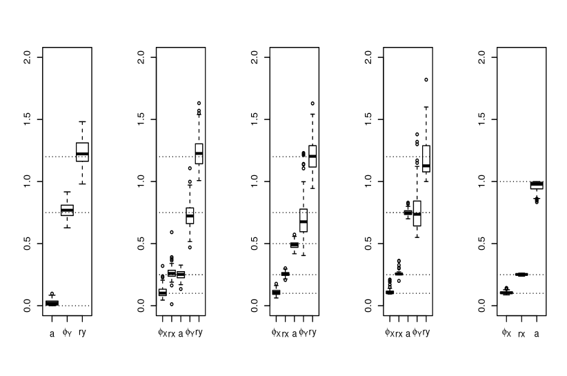
Figure 1: Boxplots of censored pairwise likelihood estimates based on 150 simulation replicates from 1000 independent copies of MM model with mixing coefficient (from left to right: $a=0,a=0.25,a=0.50,a=0.75$ and $a=1$) and $\phi_{X}=0.10,r_{X}=0.25,\phi_{Y}=0.75,r_{Y}=1.20$. Results for the unidentifiable parameters are not reported.

In order to obtain accurate estimates of $\mathcal{H}(\vartheta)$ and $\mathcal{J}(\vartheta)$ in the Monte Carlo procedure, we perform an exploratory study with 200 simulation replicates based on MM model described above with parameters $\beta_{MM}=\{\phi_{X}=0.10,r_{X}=0.25,\phi_{Y}=0.75,r_{Y}=1.2,a=0.5\}$. For each replication, we randomly generate $K=50$ locations uniformaly in the square [0, 2] $\times$[0, 2] with 1000 independent observations at each sampled location. Then, we simulate data from the fitted model with $M\in\{1000,1250,1500\}$ independent simulations at the sampled $K$ locations. In Figure 2, we present the boxplots for $G^{aa}$ and $H^{aa}$. The results give a justification to use $M=1500$ as a compromise between accuracy and computation time.

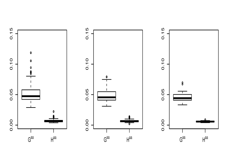
Figure 2: Boxplots for calculated matrices elements by Monte Carlo procedure based on 200 simulation replicates from 1000 independent copies of MM model with parameters $\{\phi_{X}=0.10,r_{X}=0.25,\phi_{Y}=0.75,r_{Y}=1.2,a=0.5\}$. (from left to right: $M=1000,M=1250,$ and $M=1500$ ). Results for required elements are reported.

Figure 3 and Tables 1, 2 and 3 report a summary of comparison results between the two statistics $Z$ and $LR$ in terms of empirical probabilities for concluding $H_{1}$ in testing hypothesis $H_{0}:a=a_{0}$ against $H_{1}:a\neq a_{0}$ based on 150 simulation replicates from 1000 independent copies simulated at 50 randomly and uniformaly sampled locations in the square $[0,2]^{2}$ from three MM models with parameters $\{\phi_{X}=0.10,r_{X}=0.25,\phi_{Y}=0.75,r_{Y}=1.2\}$, according to different values of the mixing parameter $a\in\{0.25,0,50,0.75\}$. Decisions obtained at three significance levels $\alpha\in\{0.01,{\color[rgb]{0,0,0}0.05},0.10\}$.

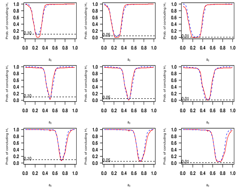
Figure 3: Empirical probabilities of concluding $H_{1}$ based on 150 replicates simulation study of three MM models with $\ X$=TEG, $\beta_{MS}=\{\phi_{X}=0.10,r_{X}=0.25\}$, and $Y$= Inverted TEG processes, $\beta_{IMS}=\{\phi_{Y}=0.75,r_{Y}=1.2\}$, the mixing coefficients (top row: $a=0.25$, middle row: $a=0.50$ and bottom row: $a=0.75$). 50 locations were randomly and uniformly generated in the square $[0,2]^{2}$, and 1000 realisations were simulated at the sampled locations. (Red solid line: $Z$ test and blue dashed line: $LR$ test).

Despite the poor performance which may be expected at the region around to the true mixing coefficient $a$. The results in terms of empirical probabilities for concluding $H_{1}$ of the two statistic show a reasonable performance. The probability of making a correct decision becomes higher as we become very close or move far from the model true value. We also remark that the performances of the two tests are very similar except for $a_{0}=0.25$, $\alpha=0.1$ where the $Z$ test presents an unexpected over sensitivity.

$a_{0}$	0.05	0.10	0.15	0.20	0.25	0.30	0.35	0.40	0.50	0.80
$\alpha$=0.01
$LR$	0.980	0.647	0.293	0.067	0.007	0.033	0.100	0.440	0.980	0.993
$Z$	0.880	0.533	0.187	0.000	0.000	0.007	0.067	0.600	0.980	0.993

$\alpha$=0.05
$LR$	0.973	0.880	0.480	0.100	0.033	0.080	0.293	0.813	0.980	0.993
$Z$	0.993	0.813	0.440	0.060	0.007	0.013	0.393	0.880	0.987	0.993

$\alpha$=0.10
$LR$	0.993	0.920	0.593	0.193	0.087	0.187	0.527	0.880	0.987	0.993
$Z$	0.960	0.900	0.533	0.167	0.007	0.067	0.600	0.96	0.993	1.000

Table 1: Summary of empirical probabilities of concluding the alternative hypothesis for testing $H_{0}:a=a_{0}$ against $H_{1}:a\neq a_{0}$ based on 150 simulation replicates from 1000 independent copies of a true model with parameters $\beta_{MM}=\{\phi_{X}=0.10,r_{X}=0.25,\phi_{Y}=0.75,r_{Y}=1.2,a=0.25\}$, at three significance levels $\alpha\in\{0.01,0.05,0.10\}$.

$a_{0}$	0.10	0.25	0.35	0.40	0.45	0.50	0.55	0.60	0.65	0.75
$\alpha$=0.01
$LR$	0.993	0.967	0.753	0.360	0.053	0.013	0.100	0.560	0.907	0.980
$Z$	0.967	0.960	0.847	0.393	0.140	0.000	0.133	0.653	0.913	0.960

$\alpha$=0.05
$LR$	1.000	0.980	0.933	0.627	0.227	0.033	0.293	0.687	0.960	1.000
$Z$	0.973	0.967	0.927	0.607	0.260	0.007	0.400	0.807	0.947	0.967

$\alpha$=0.10
$LR$	1.000	0.987	0.960	0.687	0.260	0.060	0.413	0.813	0.967	1.000
$Z$	0.980	0.967	0.960	0.760	0.320	0.020	0.540	0.867	0.960	0.967

Table 2: Summary of empirical probabilities of concluding the alternative hypothesis for testing $H_{0}:a=a_{0}$ against $H_{1}:a\neq a_{0}$ based on 150 simulation replicates from 1000 independent copies of a true model with parameters $\beta_{MM}=\{\phi_{X}=0.10,r_{X}=0.25,\phi_{Y}=0.75,r_{Y}=1.2,a=0.5\}$, at three significance levels $\alpha\in\{0.01,0.05,0.10\}$.

$a_{0}$	0.40	0.50	0.60	0.65	0.70	0.75	0.80	0.85	0.90	0.95
$\alpha$=0.01
$LR$	0.987	0.980	0.767	0.280	0.060	0.047	0.213	0.593	0.920	0.987
$Z$	0.987	0.947	0.740	0.220	0.047	0.040	0.147	0.367	0.753	0.913

$\alpha$=0.05
$LR$	0.993	0.987	0.900	0.553	0.153	0.087	0.327	0.780	0.960	1.000
$Z$	0.993	0.953	0.907	0.553	0.087	0.060	0.253	0.620	0.893	0.973

$\alpha$=0.10
$LR$	0.993	0.993	0.960	0.707	0.253	0.113	0.353	0.893	0.980	1.000
$Z$	0.993	0.960	0.967	0.673	0.187	0.107	0.307	0.727	0.920	0.993

Table 3: Summary of empirical probabilities of concluding the alternative hypothesis for testing $H_{0}:a=a_{0}$ against $H_{1}:a\neq a_{0}$ based on 150 simulation replicates from 1000 independent copies of a true model with parameters $\beta_{MM}=\{\phi_{X}=0.10,,r_{X}=0.25,\phi_{Y}=0.75,r_{Y}=1.2,a=0.75\}$, at three significance levels $\alpha\in\{0.01,0.05,0.10\}$.

We have also explored the AD and AI cases (i.e $a=1$ and $a=0$ respectively).The two tests were performed for all $a_{0}$ values in the set $\{0.01,0.02,...,0.99\}$. We have computed the probability of concluding $H_{0}:\ a=a_{0}$ while the true parameter is $1$ (AD case) or $0$ (AI case). For this purpose a MM model were fitted for each 150 simulation replicates from a MS TEG and inverted TEG processes with parameters $\beta_{MS}=\{\phi_{X}=0.10,r_{X}=0.25\}$, $\beta_{IMS}=\{r_{Y}=1.2,\phi_{Y}=0.75\}$, repectively, and a moderately sized data with $K$ = 50 sites and $M$=1000 independent observations. The spatial domains respectively are $[0,1]^{2}$ (AD case) and $[0,2]^{2}$ (AI case). The results are presented in Figure 4 and Tables 4 and 5.

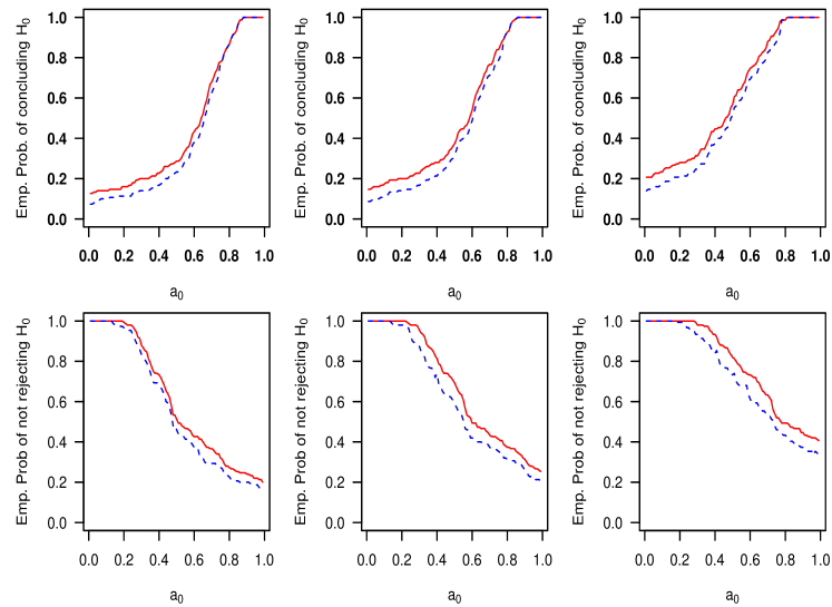
Figure 4: Empirical probabilities of concluding $H_{0}:a=a_{0}$ based on fitting a MM model to 150 simulation replicates from 1000 independent copies from TEG and inverted TEG data. ( Top row: MS data with parameters $\beta_{MS}=\{\phi_{X}=0.10,r_{X}=0.25\}$, and bottom row: IMS model with parameters $\beta_{IMS}=\{\phi_{Y}=0.75,r_{Y}=1.2\}$). $50$ locations were randomly generated and uniformaly in the square $[0,2]^{2}$ (AD case) and $[0\/,1]^{2}$ in the AI case, and $1.000$ realisations were simulated at the sampled locations. (Red solid line: $Z$ test and blue dashed line: $LR$ test). The significance levels from left to right are $\alpha=0.10$, $\alpha=0.05$, and $\alpha=0.01$.

$a_{0}$	0.01	0.10	0.20	0.30	0.40	0.50	0.60	0.70	0.80	0.90
$\alpha$=0.01
$LR$	0.140	0.173	0.213	0.247	0.373	0.513	0.693	0.820	0.987	1.000
$Z$	0.207	0.233	0.280	0.313	0.447	0.567	0.747	0.880	0.987	1.000

$\alpha$=0.05
$LR$	0.087	0.113	0.140	0.167	0.213	0.320	0.487	0.713	0.927	1.000
$Z$	0.147	0.173	0.200	0.227	0.280	0.373	0.540	0.767	0.927	1.000

$\alpha$=0.10
$LR$	0.073	0.100	0.113	0.140	0.167	0.233	0.380	0.613	0.867	1.000
$Z$	0.127	0.140	0.160	0.200	0.227	0.287	0.433	0.680	0.867	1.000

Table 4: Summary of empirical probabilities of concluding the null hypothesis for testing $H_{0}:a=a_{0}$ against $H_{1}:a\neq a_{0}$ based on 150 simulation replicates from 1000 independent copies of a true MS model with parameters $\beta_{MS}=\{\phi_{X}=0.10,r_{X}=0.25\}$, at three significance levels $\alpha\in\{0.01,0.05,0.10\}$.

$a_{0}$	0.10	0.20	0.30	0.40	0.50	0.60	0.70	0.80	0.90	0.99
$\alpha$=0.01
$LR$	1.000	0.993	0.933	0.840	0.733	0.613	0.540	0.433	0.373	0.333
$Z$	1.000	1.000	0.980	0.933	0.820	0.733	0.633	0.493	0.447	0.407

$\alpha$=0.05
$LR$	1.000	0.980	0.873	0.740	0.587	0.420	0.373	0.307	0.267	0.200
$Z$	1.000	1.000	0.953	0.813	0.693	0.493	0.433	0.373	0.313	0.253

$\alpha$=0.10
$LR$	1.000	0.967	0.833	0.680	0.487	0.367	0.293	0.220	0.200	0.167
$Z$	1.000	0.993	0.880	0.733	0.513	0.427	0.367	0.273	0.240	0.200

Table 5: Summary of empirical probabilities of concluding the null hypothesis for testing $H_{0}:a=a_{0}$ against $H_{1}:a\neq a_{0}$ based on 150 simulation replicates from 1000 independent copies of a true IMS model with parameters $\beta_{IMS}=\{\phi_{Y}=0.75,r_{Y}=1.2\}$, at three significance levels $\alpha\in\{0.01,0.05,0.10\}$.

Despite the interesting results, that show the increase of the empirical probability of concluding $H_{0}$, both tests fail to identify precisely AD or AI. They could be used as indication of AD or AI but are not sensitive.

6 Rainfall Data Example

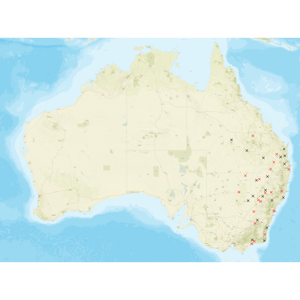
Figure 5: Geographical locations of the 38 meteorological stations located in the East of Australia. Red crosses represent stations in group A, while black ones denote group B.

The data analysed in this section are daily rainfall amounts in (millimetres) over the years 1972-2016 occurring during April-September at 38 sites in the East of Australia whose locations are shown in Fig. 5. The altitude of the sites varying from 4 to 552 meters above mean sea level. The sites are separated by distances from $34$km to $1383$km. This data set is freely avaliable on http://www.bom.gov.au/climate/data/.

Following the approach of [2], we have done a graphical exploration using the coefficients $\chi$ and $\bar{\chi}$, in order to evaluate a possible anisotropy in the data. Figure 6 is based on the empirical estimates of the functions $\chi(h,u)$ and $\bar{\chi}{(h,u)}$ in different directional sectors $(-\pi/8,\pi/8]$, $(\pi/8,3\pi/8]$, $(3\pi/8,5\pi/8]$, and $(5\pi/8,7\pi/8]$, where $0$ represents the northing direction. We can conclude that there is no evidence for anisotropy and we shall consider that the data comes from an isotropic process.

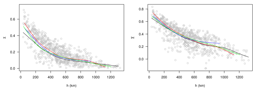
Figure 6: Pairwise empirical estimates of $\chi$ (left panel) and $\bar{\chi}$ (right panel) versus distance at threshold $u=0.970$. Grey points are empirical pairwise estimates for all data pairs. Colored lines are the loess smoothed values of the empirical estimates in different directional sectors: black line $(-\pi/8,\pi/8]$, red line $(\pi/8,3\pi/8]$, blue line $(3\pi/8,5\pi/8]$, and green line $(5\pi/8,7\pi/8]$.

A way to apply our testing approach is based on dividing the daily rainfall dataset from the 38 sites into two groups A and B (see Figure 5). We shall consider five models which belong to the three classes: MM, MS, and IMS. These models are first fitted on data from group A. The composite likelihood information criterion (CLIC) [31], defined as CLIC= $-2[p\ell(\hat{\vartheta})-tr\{\mathcal{J}(\hat{\vartheta})\mathcal{H}^{-1}(\hat{\vartheta})\}]$ is used to choose the best fitted model. Lower values of CLIC indicate a better fit. Then we apply our test with the best fitted model for group A. Let $a_{0}$ be the mixing parameter of the best fitted model for group A (we found $a_{0}=0.23$). Our test will be done on the group B data, and will be $H_{0}:a=a_{0}$ vs $H_{1}:a\neq a_{0}$.

The fitted models are:

$\mathbf{M_{1}}$: a MM model where $X$ is a TEG process with an exponential correlation function $\rho(h)=\exp(-\lVert{h}\rVert/\phi_{X})$, $\phi_{X}>0$. $\mathcal{A}_{X}$ is a disk of fixed and unknown radius $r_{X}$, and $Y$ is an inverted TEG process with exponential correlation function $\rho(h)=\exp(-\lVert{h}\rVert/\phi_{Y})$, $\phi_{Y}>0$, and $\mathcal{A}_{Y}$ is a disk with fixed and unknown radius $r_{Y}$.

$\mathbf{M_{2}}$: a MM model where $X$ is a TEG process as in $\mathbf{M_{1}}$. $Y$ is an isotropic inverted Smith process where $\Sigma$ is a diagonal matrix ($\sigma_{12}=0$) with $\sigma_{11}^{2}=\sigma_{22}^{2}=\phi_{Y}^{2}$, i.e., $\gamma(h)=(\lVert{h}\rVert/\phi_{Y})$.

$\mathbf{M_{3}}$: a MS TEG process described as $X$ in $\mathbf{M_{1}}$.

$\mathbf{M_{4}}$: a MS isotropic Smith process where $\Sigma$ is a diagonal matrix ($\sigma_{12}=0$) with $\sigma_{11}^{2}=\sigma_{22}^{2}=\phi_{X}^{2}$, i.e., $\gamma(h)=(\lVert{h}\rVert/\phi_{X})$.

$\mathbf{M_{5}}$: the inverted Smith process described as $Y$ in $\mathbf{M_{2}}$.

The considered models have unit Fréchet marginal distributions. We fit a GEV distribution on each site and then transform the marginal laws to unit Fréchet using

$${\color[rgb]{0,0,0}\hat{F}(z)=\left(1+\hat{\xi}\frac{z-\hat{\mu}}{\hat{\sigma}}\right)^{1/\hat{\xi}}\/},$$

where $(\hat{\xi},\hat{\mu},\hat{\sigma})$ are the estimated parameters of the GEV distribution. The censored pairwise likelihood approach (3.4) is used in order to estimate the parameters. The threshold is $u=-1/\log(0.90)$ and equal weights are used. The matrices $\mathcal{H}(\vartheta)$ and $\mathcal{J}(\vartheta)$ and the related quantities CLIC and standard errors are obtained by Monte Carlo procedure through simulating data with $M=1500$ independent draws at the sampled 19 sites from the fitted model.

Our results are summarised in Table 6. The best-fitting model for group A, as judged by CLIC, is the hybrid dependence model $M_{2}$. The mixing coefficient for the other hybrid model $M_{1}$ is very close to one, which indicates that there is no mixture between the max-stable process and the asymptotically independent one, so the asymptotic independence components are not identifiable. This fact affects the values of the estimates. Moreover, model $M_{1}$ reduces to model $M_{3}$.

Model	${\hat{\phi}}_{X}$	${\hat{r}}_{X}$	$\hat{{a}}$	${\hat{\phi}}_{Y}$	${\hat{r}}_{Y}$	CLIC
$M_{1}$	302.09 (67.79)	753.67 (191.02)	$\simeq 1$(0.01)	2064.71 (542.84)	970.04 (188.28)	1951654
$M_{2}$	43.77 (31.84)	94.81 (45.96)	0.23 (0.06)	1111.53 (430.98)	-	${1950330}^{*}$
$M_{3}$	303.09 (68.52)	751.44 (189.10)	-	-	-	1951654
$M_{4}$	130.05 (36.82)	-	-	-	-	1968505
$M_{5}$	-	-	-	337.40 (86.41)	-	1963187

Table 6: Parameter estimates of selected dependence models fitted to the daily rainfall data from group A, along with the composite likelihood criterion (CLIC) and standard errors reported between parentheses.

For data from group B, we have considered the two statistics $Z$ and $LR$ described in this paper, to test if the hybrid model $M_{2}$ can be used to make inference for this group, i.e., testing $H_{0}:a=0.23$ versus $H_{1}:a\neq 0.23$. We obtain the calculated values for $Z$ and $LR$, $Z=0.73$ ($p-$value$=0.47$), ${LR=7.72}$, $\lambda=14.07$, ($p-$value$={0.458}$).

This leads us to retain $H_{0}$ and thus that there is no differences in the mixing parameter between the two groups. We have also performed an independent two-samples $Z$-test: let $a_{A}$ (resp. $a_{B}$ be the mixing parameter for group A (resp. group B), consider $H_{0}:a_{A}=a_{B}$. The statistic

$$Z_{C}=\frac{\hat{a}_{A}-\hat{a}_{B}}{SE_{\hat{a}_{A}-\hat{a}_{B}}}$$

where $SE$ stands for the estimated standard error. The calculated value of $Z_{C}$ is $0.17$ with $p$-value $=0.86$, leading to retain $H_{0}$ and conclude that there is no significant difference between the two mixing coefficient.
Nevertheless, these conclusions are subordinated to the assumption that both groups A and B have the same underlying model M2.

7 Conclusion

In this paper we have considered hypothesis testing for the mixing coefficient of a MM models proposed in [32] using two statistics the $Z$ and the $LR$ when a censored pairwise likelihood is employed for inferential purposes.

The two statistics has emerged as an efficient tools for testing hypothesis on the mixing coefficient with better performance achieved by $LR$, but with the drawback of a nonstandard asymptotic distribution at the boundaries, since the number of nuisance parameters is different between the two hypothesis and it also requires heavier computations. Our procedure seems to be a performant validation tool.

One other drawback of our work is that the proposed tests model-dependent. In the future, we plan to propose a free-model test, using the F-madogram.
 
 
Acknowledgments. We are grateful to Jean-Noël Bacro, Carlo Gaetan and Gwladys Toulemonde for giving their estimations C codes which we used as a base for computing the statistics of our tests. This work was supported by the LABEX MILYON (ANR-10-LABX-0070) of Université de Lyon, within the program ”Investissements d’Avenir” (ANR-11-IDEX-0007) operated by the French National Research Agency (ANR). It was also supported by the CERISE LEFE-INSU projcet.

References

- [1] Jean-Noël Bacro, Liliane Bel, and Christian Lantuéjoul. Testing the independence of maxima: from bivariate vectors to spatial extreme fields. Extremes, 13(2):155–175, 2010.
- [2] Jean-Noel Bacro, Carlo Gaetan, and Gwladys Toulemonde. A flexible dependence model for spatial extremes. Journal of Statistical Planning and Inference, 172:36–52, 2016.
- [3] Manuela Cattelan and Nicola Sartori. Empirical and simulated adjustments of composite likelihood ratio statistics. Journal of Statistical Computation and Simulation, 86(5):1056–1067, 2016.
- [4] Richard E Chandler and Steven Bate. Inference for clustered data using the independence loglikelihood. Biometrika, pages 167–183, 2007.
- [5] Stuart Coles, Janet Heffernan, and Jonathan Tawn. Dependence measures for extreme value analyses. Extremes, 2(4):339–365, 1999.
- [6] Dan Cooley, Philippe Naveau, and Paul Poncet. Variograms for spatial max-stable random fields. Dependence in probability and statistics, pages 373–390, 2006.
- [7] Robert B Davies. Hypothesis testing when a nuisance parameter is present only under the alternative. Biometrika, 64(2):247–254, 1977.
- [8] Robert B Davies. Hypothesis testing when a nuisance parameter is present only under the alternatives. Biometrika, pages 33–43, 1987.
- [9] AC Davison and MM Gholamrezaee. Geostatistics of extremes. In Proc. R. Soc. A, volume 468, pages 581–608, 2012.
- [10] Anthony C Davison, Raphaël Huser, and Emeric Thibaud. Geostatistics of dependent and asymptotically independent extremes. Mathematical Geosciences, 45(5):511–529, 2013.
- [11] Anthony C Davison, Simone A Padoan, and Mathieu Ribatet. Statistical modeling of spatial extremes. Statistical science, pages 161–186, 2012.
- [12] L. De Haan and T. T. Pereira. Spatial extremes: Models for the stationary case. The annals of statistics, pages 146–168, 2006.
- [13] Laurens De Haan. A spectral representation for max-stable processes. The annals of probability, pages 1194–1204, 1984.
- [14] Helena Geys, Geert Molenberghs, and Louise M Ryan. Pseudolikelihood modeling of multivariate outcomes in developmental toxicology. Journal of the American Statistical Association, 94(447):734–745, 1999.
- [15] Raphaël Huser and AC Davison. Space–time modelling of extreme events. Journal of the Royal Statistical Society: Series B (Statistical Methodology), 76(2):439–461, 2014.
- [16] Harry Joe. Parametric families of multivariate distributions with given margins. Journal of multivariate analysis, 46(2):262–282, 1993.
- [17] Zakhar Kabluchko, Martin Schlather, and Laurens De Haan. Stationary max-stable fields associated to negative definite functions. The Annals of Probability, pages 2042–2065, 2009.
- [18] John T Kent. Robust properties of likelihood ratio tests. Biometrika, 69(1):19–27, 1982.
- [19] Diego Kuonen. Miscellanea. saddlepoint approximations for distributions of quadratic forms in normal variables. Biometrika, 86(4):929–935, 1999.
- [20] Anthony W Ledford and Jonathan A Tawn. Statistics for near independence in multivariate extreme values. Biometrika, 83(1):169–187, 1996.
- [21] Bruce G Lindsay. Composite likelihood methods. Contemporary mathematics, 80(1):221–39, 1988.
- [22] Thomas Opitz. Extremal t processes: Elliptical domain of attraction and a spectral representation. Journal of Multivariate Analysis, 122:409–413, 2013.
- [23] Luigi Pace, Alessandra Salvan, and Nicola Sartori. Adjusting composite likelihood ratio statistics. Statistica Sinica, pages 129–148, 2011.
- [24] Simone A Padoan, Mathieu Ribatet, and Scott A Sisson. Likelihood-based inference for max-stable processes. Journal of the American Statistical Association, 105(489):263–277, 2010.
- [25] Andrea Rotnitzky and Nicholas P Jewell. Hypothesis testing of regression parameters in semiparametric generalized linear models for cluster correlated data. Biometrika, pages 485–497, 1990.
- [26] Martin Schlather. Models for stationary max-stable random fields. Extremes, 5(1):33–44, 2002.
- [27] Richard L Smith. Max-stable processes and spatial extremes. Unpublished manuscript, 205, 1990.
- [28] E Thibaud, R Mutzner, and AC Davison. Threshold modeling of extreme spatial rainfall. Water resources research, 49(8):4633–4644, 2013.
- [29] Cristiano Varin. On composite marginal likelihoods. AStA Advances in Statistical Analysis, 92(1):1–28, 2008.
- [30] Cristiano Varin, Nancy Reid, and David Firth. An overview of composite likelihood methods. Statistica Sinica, pages 5–42, 2011.
- [31] Cristiano Varin and Paolo Vidoni. A note on composite likelihood inference and model selection. Biometrika, pages 519–528, 2005.
- [32] Jennifer L. Wadsworth and Jonathan A. Tawn. Dependence modelling for spatial extremes. Biometrika, 99(2):253, 2012.