Learning 2D Gabor Filters by Infinite Kernel Learning Regression

Abstract

Gabor functions have wide-spread applications in image processing and computer vision. In this paper, we prove that 2D Gabor functions are translation-invariant positive-definite kernels and propose a novel formulation for the problem of image representation with Gabor functions based on infinite kernel learning regression. Using this formulation, we obtain a support vector expansion of an image based on a mixture of Gabor functions. The problem with this representation is that all Gabor functions are present at all support vector pixels. Applying LASSO to this support vector expansion, we obtain a sparse representation in which each Gabor function is positioned at a very small set of pixels. As an application, we introduce a method for learning a dataset-specific set of Gabor filters that can be used subsequently for feature extraction. Our experiments show that use of the learned Gabor filters improves the recognition accuracy of a recently introduced face recognition algorithm.

1 Introduction

Gabor functions are extensively used for feature extraction in numerous computer vision applications such as face recognition[7, 36, 47, 28, 45], image retrieval [25], palmprint recognition[34, 33], forgery detection[23], and facial expression recognition[46, 19]. Neurologists have shown that receptive field of simple cortical cells can be modeled with Gabor functions[10, 11, 29]. For this reason, computational models for visual recognition that have inspired from visual cortex use Gabor filters in the very beginning phase of feature extraction [40]. Even nowadays that deep learning methods have remarkably influenced the field of machine vision, the combination of Gabor functions and convolutional neural networks(CNN) has been observed to improve recognition rates[8].

In this paper, we show that Gabor functions are translation-invariant (also called stationary) positive-definite kernels. It is somewhat strange that this fact, despite its simple proof, has been invisible to the eyes of researchers and it is neither mentioned in classical books such as [39, 9, 41] nor in seminal work of Genton [15] who reviewed the class of stationary kernels. We believe that the positive-definiteness of Gabor functions can potentially be exploited in numerous ways for applying kernel algorithms to machine vision problems. In this paper, we target the problem of learning Gabor filters from data which in kernel methods terminology is a kernel learning problem. Perhaps the most widespread kernel learning algorithm is the multiple kernel learning (MKL) framework that seeks the best convex combination of a finite set of kernel functions[22, 3, 42, 35, 44, 21, 6]. One weakness of the MKL framework is that the initial set of kernel functions should be chosen by hand. To overcome this limitation, the infinite kernel learning (IKL) framework was introduced in which the set of initial kernels is extended to an infinite number of kernels parameterized over a continuous space [30, 1, 2, 14, 32, 31, 17]. Some of the solutions proposed for this problem were restricted to Gaussian kernels [30, 1, 2] and some were restricted to binary classification with support vector machines [14, 32, 31, 17]. However, to apply these IKL algorithms to the problem of learning Gabor functions, one should formulate the problem of learning Gabor functions as binary classification which seems to be impossible. Fortunately, Ghiasi-Shirazi [18] generalized the SIKL algorithm[17] to a more general class of machine learning problems that includes the $\epsilon$-insensitive support vector regression (SVR). In this paper, we reduce the problem of representing an image with Gabor functions to the problem of learning a convex combination of an infinite number of Gabor kernels for regression. This gives us a mixture of Gabor functions that, when placed at positions determined by support vectors, reconstruct the given image. As a practical application of the SIKL algorithm, we propose a simple method for learning Gabor functions for a specific dataset of images from a tiny fraction of its images. However, the representation obtained by the SIKL algorithm has the problem that all Gabor functions are present at all support vector pixels. This may arouse the suspicion that the SIKL algorithm learns a universal approximator kernel function that is subsequently used by SVR for representing the input image, rejecting any link between the Gabor functions generating an image and the learned Gabor functions. In fact, we will show experimentally that the mixture of Gabor functions learned by the SIKL algorithm is approximately a highly concentrated Laplacian kernel. Using LASSO algorithm [43], we obtain a sparse representation of the original image in which the Gabor functions are located at a very sparse set of pixels. Experimental results on artificial images generated by combination of two Gabor functions confirm the potential of our sparse representation algorithm in discovering the scales, orientations, and locations of the constituting Gabor functions.

In Section 2, we give a concise and simplified introduction to SIKL regression [the general form of SIKL algorithm and its mathematical analysis can be found in 18]. We introduce our method for representing an image as a mixture of Gabor functions in Section 3. Our algorithm for choosing the parameters of Gabor filters for a specific dataset is given in Section 4. In Section 5, we show how LASSO can be utilized to obtain a sparse Gabor-based representation of an image. We experimentally evaluate the proposed method in Section 6 and conclude the paper in Section 7. In A, we give a formal proof for positive-definiteness of Gabor functions.

2 Stabilized infinite kernel learning regression

The stabilized infinite kernel learning (SIKL) algorithm had been initially introduced in [17] for binary classification and then was generalized to more general classes of machine learning problems in [18]. In this section, we give a short introduction to SIKL regression in a simple and succinct way without going into mathematical details and without grounding the SIKL framework in its most general form. For a comprehensive introduction to the SIKL framework the reader is referred to [18].

Assume that the training set consists of the input samples $x_{1},...,x_{l}\in\mathbb{R}^{d}$ and their corresponding target values $y_{1},...,y_{l}\in\mathbb{R}$. Support vector regression attempts to learn the relation between input and output by a function of the form:

$$f(x)=\sum_{i=1}^{l}(\hat{\beta}_{i}-\beta_{i})k(x_{i},x)+b.$$ (1)

The coefficients $\hat{\beta}$ and $\beta$ are obtained by solving the following optimization problem [9]:

$$\max_{\hat{\beta},\beta} \sum_{i=1}^{l}y_{i}(\hat{\beta}_{i}-\beta_{i})-\epsilon\sum_{i=1}^{l}(\hat{\beta}_{i}+\beta_{i})$$

$$-\frac{1}{2}\sum_{i=1}^{l}\sum_{j=1}^{l}(\hat{\beta}_{i}-\beta_{i})(\hat{\beta}_{j}-\beta_{j})k(x_{i},x_{j})$$

$$s.t. 0\leq\hat{\beta}_{i},\beta_{i}\leq C\;\;\;\textsf{for}\;\;\;i=1,...,l$$

$$\sum_{i=1}^{l}(\hat{\beta}_{i}-\beta_{i})=0$$

where $C\in(0,\infty]$ is a regularization constant. The above optimization problem can be rewritten in the following more succinct form:

$$\max_{\alpha\in\mathcal{A}}-\frac{1}{2}\alpha^{T}A^{T}KA\alpha-c^{T}\alpha$$ (3)

where $K$ is the kernel matrix obtained by applying the kernel function $k$ to the input samples $x_{1},...,x_{l}$,

$$\begin{aligned} &\alpha=\begin{bmatrix}\hat{\beta}\\ \beta\end{bmatrix},\\ &A=\begin{bmatrix}I_{\ell}\\ -I_{\ell}\end{bmatrix}^{T},\\ &c=\begin{bmatrix}y_{1}\;\;y_{2}\;\;\ldots\;\;y_{\ell}\;\;-y_{1}\;\;-y_{2}\;\;\ldots\;\;-y_{\ell}\end{bmatrix}^{T}-\varepsilon,\\ &\mathcal{A}=\left\{\alpha|\alpha=\begin{bmatrix}\hat{\beta}\\ \beta\end{bmatrix},\;0\leq\alpha_{i}\leq C,\;\sum_{i=1}^{\ell}(\hat{\beta}_{i}-\beta_{i})=0\right\},\end{aligned}$$ (4)

and $I_{\ell}$ is the identity matrix of size $\ell$.

Consider the set of kernels $\left\{k_{\gamma}:\gamma\in\Gamma\right\}$, where $\Gamma$ is a continuously parameterized index set. Let $\mathcal{P}(\Gamma)$ be the set of all probability measures on $\Gamma$. It can be shown [see 30] that for any probability measure $p\in\mathcal{P}(\Gamma)$, the function

$$\hat{k}_{p}(x,z)=\int_{\Gamma}k_{\gamma}(x,z){\,\mathrm{d}}p(\gamma)$$ (5)

is a convex combination of the set of kernels $\left\{k_{\gamma}:\gamma\in\Gamma\right\}$. Conversely, any convex combination of the set of kernels $\left\{k_{\gamma}:\gamma\in\Gamma\right\}$ can be written in the form of Eq. (5). In the IKL framework, it is assumed that $\Gamma$ is a compact Hausdorff space (e.g. a bounded and closed subset of $\mathbb{R}^{2}$) and the problem is to find the best kernel in the form of Eq. (5). The SIKL framework relaxes the assumption on $\Gamma$ to locally-compact Hausdorff spaces (e.g. $\mathbb{R}$ or $\mathbb{R}^{2}$). For mathematical concreteness and for provisioning a mechanism to control the capacity of the learning machine, the SIKL framework introduces a vanishing function $G(\gamma):\Gamma\rightarrow[0,1]$ into the framework. The stabilized convex combination of the kernels $\left\{k_{\gamma}:\gamma\in\Gamma\right\}$ with stabilizer $G(\gamma)$ and probability measure $p\in\mathcal{P}(\Gamma)$ is defined as:

$$\bar{k}_{p}(x,z)=\int_{\Gamma}k_{\gamma}(x,z)G(\gamma){\,\mathrm{d}}p(\gamma).$$ (6)

Correspondingly, the set of stabilized convex combination of kernels $\left\{k_{\gamma}:\gamma\in\Gamma\right\}$ with stabilizer $G(\gamma)$ is defined as:

$${\mathcal{K}}:=\left\{\bar{k}_{p}:p\in\mathcal{P}(\Gamma)\right\}.$$ (7)

The problem of simultaneously learning the regression function along with a kernel function $\bar{k}_{p}\in{\mathcal{K}}$ can be formulated as:

$$\sup_{p\in\mathcal{P}(\Gamma)}\min_{\alpha\in\mathcal{A}}\left\{\int_{\gamma\in\Gamma}\left[G(\gamma)\alpha^{T}A^{T}K(\gamma)A\alpha+c^{T}\alpha\right]{\,\mathrm{d}}p(\gamma)\right\}$$ (8)

where $K(\gamma)$ is the kernel matrix that is obtained by applying the kernel function $k_{\gamma}$ to the input training data $x_{1},...,x_{l}$.

Ghiasi-Shirazi [18] proved that the probability measure that optimizes the above problem is discrete with finite support. The SIKL toolbox optimizes the above problem by semi-infinite programming and returns the weights $\mu_{i}$ and the parameters $\gamma_{i}\in\Gamma$ which identify the optimal kernel $\bar{k}$ by the following formula:

$$\bar{k}(x,z)=\sum_{i=1}^{m}\mu_{i}k_{\gamma_{i}}(x,z).$$ (9)

We added the Gabor kernel to the SIKL toolbox and exploited some special properties of Gabor kernels to optimize the toolbox. Specifically, since Gabor kernels are two-dimensional, we modified the global optimization algorithm of SIKL to search the space of parameters systematically.

3 Gabor-based image representation using SIKL

In this section, we show how SIKL regression can be applied to the task of image representation by Gabor functions. We consider the following form for Gabor functions which is essentially a slightly modified version of the from chosen by [36]:

$$\begin{aligned} \Psi&(x,y;x_{0},y_{0},\omega,\theta)=\\ &e^{-\frac{\omega^{2}((x-x_{0})^{2}+(y-y_{0})^{2})}{8\pi^{2}}}cos{\left(\omega((x-x_{0})cos{\theta}+(y-y_{0})sin{\theta})\right)}\end{aligned}$$ (10)

where the point $(x_{0},y_{0})$ is the center of the Gabor function in the spatial domain and the parameters $\omega$ and $\theta$ determine the scale and orientation of Gabor function, respectively. Note that, in Eq. (10), the only inputs are $x$ and $y$ and $x_{0}$ and $y_{0}$ are parameters of the Gabor function. By considering $x_{0}$ and $y_{0}$ as inputs, we arrive at the following definition for Gabor kernels:

$$\begin{aligned} k_{\omega,\theta}&([x,y],[x^{\prime},y^{\prime}])=\Psi(x,y;x^{\prime},y^{\prime},\omega,\theta).\end{aligned}$$ (11)

There is another parameterization for Gabor functions which is obtained from Eq. (10) by setting $\omega=\frac{\pi/2}{2^{\nu/2}}$ and $\theta=\mu\frac{\pi}{8}$. This $\mu\nu$-parameterization is specially important since manual selection of Gabor parameters is usually done in that form. We use this form when a parameter is to be chosen by hand or when reporting the learned parameters of Gabor functions. A elaborates on the chosen form for Gabor functions and gives a proof for positive-definiteness of Gabor kernels.

Now, assume that we want to search for the best convex combination of Gabor kernels whose scale parameters are in the range $[\omega_{\ell 1},\omega_{u1}]$. This choice corresponds to a rectangular vanishing function in SIKL formulation which is not appropriate due to the jumps from $0$ to $1$ and vise versa. Therefore, we choose the following trapezoidal stabilizing function:

$$G(\omega,\theta)=\left\{\begin{array}[]{llll}&0&&\omega<\omega_{\ell 0}\\ &\frac{\omega-\omega_{\ell 0}}{\omega_{\ell 1}-\omega_{\ell 0}}&&\omega_{\ell 0}<\omega<\omega_{\ell 1}\\ &1&&\omega_{\ell 1}<\omega<\omega_{u1}\\ &\frac{\omega-\omega_{u0}}{\omega_{u1}-\omega_{u0}}&&\omega_{u1}<\omega<\omega_{u0}\\ &0&&\omega>\omega_{u0}\\ \end{array}\right.$$ (17)

The stabilized convex combination of Gabor functions with stabilizer $G(\omega,\theta)$ and probability measure $p$ is defined as:

$$\begin{aligned} \bar{k}_{p}&([x,y],[x^{\prime},y^{\prime}])\\ &=\int_{\mathbb{R}^{2}}k_{\omega,\theta}([x,y],[x^{\prime},y^{\prime}])G(\omega,\theta){\,\mathrm{d}}p(\omega,\theta).\end{aligned}$$ (18)

Consequently, the set of stabilized convex combination of Gabor functions with stabilizer $G(\omega,\theta)$ can be expressed as:

$${\mathcal{K}}:=\left\{\bar{k}_{p}:p\in\mathcal{P}(\mathbb{R}^{2})\right\}.$$ (19)

As stated previously, although the optimization is over a continuous space of parameters, the optimal kernel has a finite expansion of the form:

$$\bar{k}([x,y],[x^{\prime},y^{\prime}])=\sum_{i=1}^{m}\mu_{i}k_{\omega_{i},\theta_{i}}(x-x^{\prime},y-y^{\prime}).$$ (20)

For a given image $I$, we generate a training set that consists of positions of pixels as input and the intensity at those pixels as desired outputs. We then use the SIKL regression algorithm to learn the above kernel and the parameters of a SVR machine simultaneously in order to predict the intensity of each pixel correctly. The solution of the SIKL problem gives the number of participating kernels $m$, Gabor parameters $\omega_{i}$ and $\theta_{i}$ for $i=1,...,m$, and the support vector coefficients $\hat{\beta}_{i},\beta_{i}$ for $i=1,...,\ell$, where $\ell$ is the number of pixels in the image, such that:

$$I(x,y)\approx\sum_{i\in SV}{(\hat{\beta}_{i}-\beta_{i})\sum_{j=1}^{m}{\mu_{j}k_{\omega_{j},\theta_{j}}(x-x_{i},y-y_{i})}}+b.$$ (21)

This representation signifies the Gabor functions that are contributing to the construction of the input image $I$.

4 Learning dataset-specific Gabor filters

When Gabor filters are used for feature extraction from a dataset, their parameters are usually tuned by hand and it is customary to use 40 Gabor functions with 5 scales and 8 directions[27, 26, 36, 20]. However, since Gabor functions are defined over a pixel-space, appropriate choice of their parameters is sensitive to the resolution of the images. In Section 3, we proposed an algorithm for learning an image representation based on Gabor functions by SIKL. It is an accepted practice in machine learning that the first phases of information processing usually model the distribution of the input data while the task of discrimination is assigned to higher layers [5, 12]. So, we take the assumption that the Gabor functions that are appropriate for representing an image, can also be used for feature extraction. By clustering the parameters obtained from a small fraction of images from a dataset using the k-means algorithm, we obtain a set of Gabor functions that are appropriate for representing any image in that dataset. Dataset-specific details on our method for learning Gabor filters for CMU-PIE and EYaleB datasets are given in Section 6.1.

5 Sparse image representation using Gabor kernels

The Gabor kernels learned by the method proposed in the previous section are global in the sense that each kernel is present at every location. In Section 6.2 we show that the mixture of the learned Gabor functions is approximately a concentrated Laplacian kernel. It may be questioned whether the Gabor kernels learned by the SIKL algorithm are those that are actually participating in the generation of an image or the learned combined concentrated Laplacian kernel acts as a universal approximator function that can be utilized by the SVR machine for approximating any input image. In this section, we aim to represent an image sparsely by a combination of Gabor functions such that each Gabor function is located at a small number of pixels. It has the benefit that it associates Gabor functions to the specific locations at which they are present. This problem has been previously considered by Fischer et al. [13] who proposed an algorithm based on local competition. It must be mentioned that the set of Gabor functions chosen by the SIKL algorithm is already sparse. This sparseness is the result of the implicit $L1$ constraint $\lVert p\rVert_{1}=1$ over the probability measure $p$ in Eq. (8) which holds since the Lebesgue integral of any probability measure is 1. Thus, we assume that all the Gabor kernels that are found by the SIKL algorithm should be present in the sparse representation as well. We then try to sparsify the set of pixels at which each kernel is present. We start from Eq. (21) obtained in the previous section. By exchanging the order of summation we obtain:

$$I(x,y)\approx\sum_{j=1}^{m}\sum_{i\in SV}{[\mu_{j}(\hat{\beta}_{i}-\beta_{i})]k_{\omega_{j},\theta_{j}}(x-x_{i},y-y_{i})}+b.$$ (22)

Our goal is to approximate the inner summation with a sparse combination of the training input data. Let $b^{j}$ be an $\ell\times 1$ vector whose n’th element is:

$$b^{j}_{n}=\sum_{i\in SV}{[\mu_{j}(\hat{\beta}_{i}-\beta_{i})]k_{\omega_{j},\theta_{j}}(x_{n}-x_{i},y_{n}-y_{i})}.$$ (23)

Assume $K^{j}$ is the $\ell\times\#sv$ kernel matrix associated with the kernel function $k_{\omega_{j},\theta_{j}}$ in which rows correspond to the image coordinates and columns correspond to the support vector image coordinates. According to Eq. (22), to obtain a sparse representation for image $I$, we should find a sparse vector $\rho^{j}$ such that, for $n=1,...,\ell$, we have:

$$\begin{aligned} b^{j}_{n}&=\sum_{i\in SV}{[\mu_{j}(\hat{\beta}_{i}-\beta_{i})]k_{\omega_{j},\theta_{j}}(x_{n}-x_{i},y_{n}-y_{i})}\\ &\approx\sum_{i\in SV}{\rho^{j}_{i}k_{\omega_{j},\theta_{j}}(x_{n}-x_{i},y_{n}-y_{i})}.\end{aligned}$$ (24)

Eq. (24) can be written in the matrix notation as:

$$b^{j}\approx K^{j}\rho^{j}.$$ (25)

We have:

$$\begin{aligned} I(x_{n},y_{n})&\approx\sum_{j=1}^{m}\sum_{i\in SV}{[\mu_{j}(\hat{\beta}_{i}-\beta_{i})]k_{\omega_{j},\theta_{j}}(x_{n}-x_{i},y_{n}-y_{i})}+b\\ &=\sum_{j=1}^{m}{b^{j}_{n}}+b\approx\sum_{j=1}^{m}{K^{j}_{n*}\rho^{j}}+b\\ &=\sum_{j=1}^{m}\sum_{i\in SV}{\rho^{j}_{i}k_{\omega_{j},\theta_{j}}(x_{n}-x_{i},y_{n}-y_{i})}+b\end{aligned}$$ (26)

where $K^{j}_{n*}$ is the n’th row of the kernel matrix $K^{j}$ and sparseness of this representation follows from the sparseness of the vector $\rho^{j}$. To find a sparse vector $\rho^{j}$ that satisfies Eq. (25), we use LASSO[43] which solves the following optimization problem:

$$\min_{\rho^{j}}\left\{\frac{1}{\ell}\left\lVert b^{j}-K^{j}\rho^{j}\right\lVert_{2}^{2}+\lambda\left\lVert\rho^{j}\right\rVert_{1}\right\}.$$ (27)

To undo the negative effect of the $L1$ regularization term in LASSO on the quality of approximation of Eq. (25), we again solve Eq. (25) using the least squares method with the constraint that the pattern of sparseness of $\rho^{j}$ found by LASSO would be preserved.

6 Experiments

The experiments of this section are designed with two goals in mind. First, we want to analyze the proposed algorithm in details and discover the nature of the learned Gabor functions. Second, we want to show the usefulness of the proposed method in automatic learning of Gabor functions for a given dataset. In Section 6.1, we report our experiments on the application of the learned Gabor functions to the face recognition problem and show that it yields favorable recognition accuracy over a hand-tuned choice made by experts. In Section 6.2, we analyze the learned Gabor functions and show that the weighted combination of learned Gabor kernels is equivalent to a concentrated Laplacian kernel. Finally, in Section 6.3, we analyze the proposed algorithm for Gabor-based sparse representation of images.

6.1 Selection of Gabor filter for face recognition

In this section, we want to show that use of Gabor filters learned by the method proposed in Section 4 can increase the accuracy of machine vision applications compared with Gabor filters chosen by hand. For this purpose, we chose the MOST system that is recently proposed by Ren et al. [36] for the task of face recognition and uses Gabor filters for feature extraction. The code of the MOST algorithm along with the CMU-Light and EYaleB face datasets were obtained by contacting Ren et al. [36]. CMU-Light is the name [36] gave to the illumination part of CMU-PIE dataset [4] which consists of 43 images captured at different illumination conditions from 68 persons, amounting to 2924 images. The Extended Yale B dataset [16], which is abbreviated as EYaleB, consists of 64 frontal images from 38 persons again taken at different illumination conditions, amounting to 2432 images. Ren et al. [36] removed the 5 most dark images from the original 64 instances provided for each person in Extended Yale B dataset. In addition, all images had been histogram-equalized and were resized to width 46 and height 56.

Since the SIKL algorithm is time-consuming, considering the locality of Gabor functions, instead of representing a whole image with Gabor functions, we break images into several smaller (sometimes overlapping) regions and represent each region with a set of Gabor functions. From each face, we extract four regions around the two eyes, the nose, and the mouth (see Figure 1). We used a trapezoidal vanishing function in the formulation of the SIKL algorithm with $\omega_{\ell 0}=\frac{\pi}{512}$, $\omega_{\ell 1}=\frac{\pi\sqrt{2}}{512}$, $\omega_{u1}=2\sqrt{2}\pi$, and $\omega_{u0}=4\pi$. In $\mu\nu$-space, these choices correspond to $\nu_{\ell 0}=16$, $\nu_{\ell 1}=15$, $\nu_{u1}=-5$, and $\nu_{u0}=-6$.

From each dataset, we randomly selected 28 images (which in both cases amounts to less than $2\%$ of the data) for learning the parameters of Gabor filters. We used the kmeans algorithm to cluster the Gabor parameters extracted from these $28$ images to obtain $40$ Gabor filters. Finally, we evaluated the original and learned Gabor filters on the task of face recognition using the MOST method. The number of training images used by the MOST algorithm, called ntrain, is an important factor in the accuracy of the face recognition system. We compare the accuracies obtained by the original $40$ filters used by Ren et al. [36] and the $40$ filters learned by our method. Each experiment is repeated $30$ times. The results of these experiments are summarized in Table 1. As can be seen, when the number of training images for the MOST algorithm is low, use of the learned Gabor filters significantly increases the recognition rate. Figure 2 shows the parameters of the original and the learned filters in the $\mu\nu$-space. It is clear from the figure that the parameters of Gabor filters used by Ren et al. [36] do not cover the whole region of parameters that are indeed required for representing images with Gabor functions. In addition, the dataset-specific distributions for Gabor kernel parameters depicted in Figures 2.b and 2.c can be used as a guideline for manual tuning of parameters of Gabor filter.

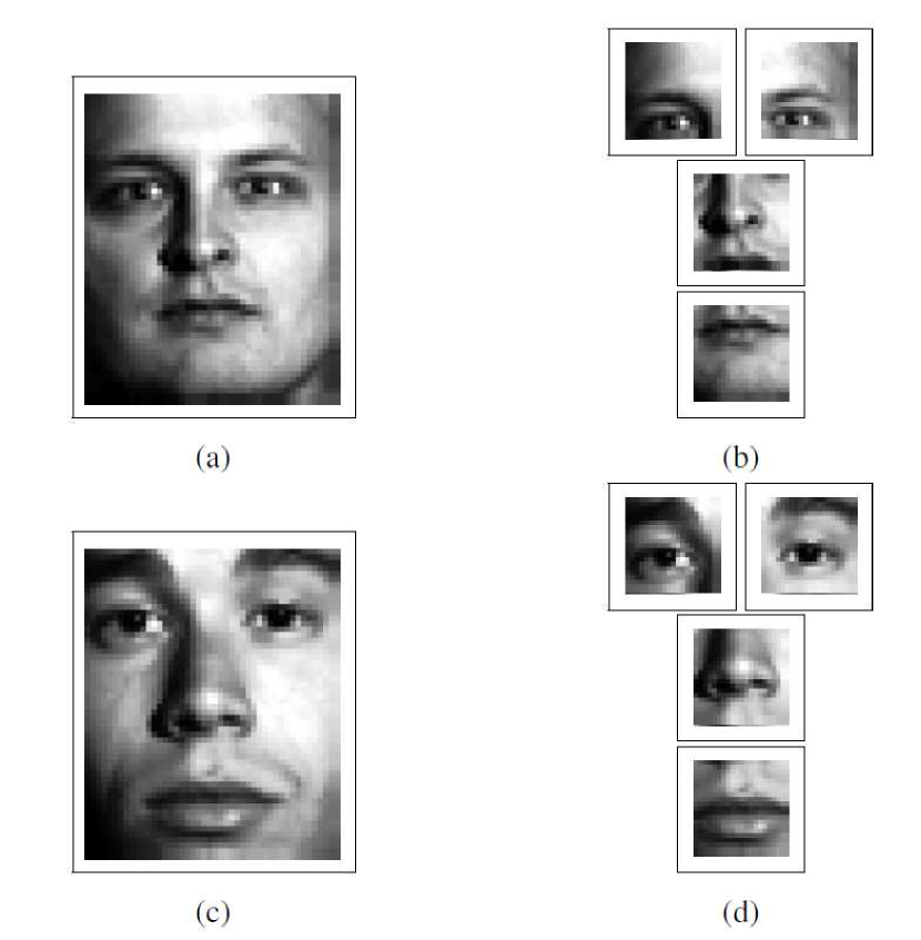
Figure 1: Regions for extracting subimages from face images. Note that two regions are overlapping. (a) and (b): An image from CMU-Light dataset and its associated subimages. (c) and (d): An image from EYaleB dataset and its associated subimages.

Table 1: Comparison of accuracies obtained by MOST algorithm on CMU-Light and EYaleB datasets when using the manually tuned Gabor filters of Ren et al. [36] and when using Gabor filters learned by the proposed algorithm. The parameter ”ntrain refers to the number of training faces used by the MOST face recognition algorithm[36]. The proposed method uses less than $2\%$ of images of each dataset for learning the parameters of Gabor kernels. For each dataset, the last column shows the two-tailed P-values for paired t-test. Results that are statistically significant are bold-faced. It must be emphasized that since a paired t-test is used, P-values cannot be computed from statistics summarized in this table.

	CMU-Light
ntrain	manually tuned	learned	P-value
1	$\mathbf{79.13\pm 5.7001}$	$\mathbf{81.66\pm 5.62}$	$\mathbf{<0.0001}$
2	$\mathbf{91.15\pm 5.8534}$	$\mathbf{92.18\pm 5.37}$	$\mathbf{0.0016}$
3	$97.39\pm 4.0537$	$97.54\pm 3.74$	$0.4522$
4	$98.95\pm 2.0855$	$98.90\pm 1.91$	$0.2268$
5	$\mathbf{99.47\pm 1.1044}$	$\mathbf{99.36\pm 1.13}$	$\mathbf{0.040}$

	EYaleB
ntrain	manually tuned	learned	P-value
1	$\mathbf{37.65\pm 2.99}$	$\mathbf{39.96\pm 3.89}$	$\mathbf{<0.0001}$
2	$\mathbf{72.99\pm 2.88}$	$\mathbf{73.71\pm 2.90}$	$\mathbf{0.0089}$
3	$88.22\pm 2.45$	$88.46\pm 2.03$	$0.2840$
4	$94.42\pm 1.72$	$94.36\pm 1.55$	$0.6407$
5	$97.09\pm 1.00$	$96.99\pm 0.96$	$0.3836$

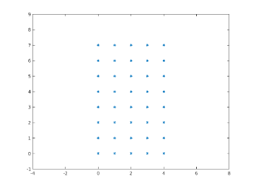
(a) Parameters of the original $40$ Gabor functions used by Ren et al. [36].

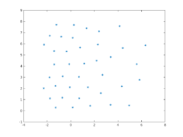
(b) Parameters of the $40$ learned Gabor functions for the CMU-Light dataset.

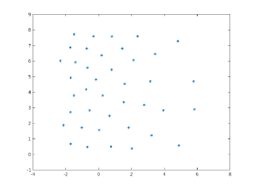
(c) Parameters of the $40$ learned Gabor functions for the EYaleB dataset.

Figure 2: Parameters of handy and learned Gabor functions depicted in $\mu\nu$-space. The horizontal axis shows the scale ($\nu$) and the vertical axis shows the orientation ($\mu$).

6.2 Analysis of the learned Gabor functions

In Section 3, we showed how the SIKL algorithm can be exploited for representing an image with Gabor kernels. The learned representation can be equivalently obtained by support vector regression with a single kernel that is the weighted combination of the selected Gabor kernels (see Eq. 20). An interesting question is what is the single kernel that is equivalent to the combination of the learned Gabor functions. We answer this question empirically by drawing the shape of the combined kernel. Figure 3 shows the combined kernels for two sample images from CMU-Light and EYaleB datasets. As can be seen, the weighted combination of the learned Gabor functions is approximately a concentrated Laplacian kernel.

(a) Learned combined kernel for a sample image region from CMU-Light dataset.

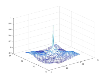
(b) Learned combined kernel for a sample image region from EYaleB dataset.

Figure 3: Compound kernels corresponding to the weighted combination of learned Gabor kernels by the method of Section 3.

6.3 Discovering locations of constituting Gabor functions

In this section, we experimentally evaluate the SIKL+LASSO algorithm of Section 5 in discovering the exact location of Gabor functions participating in a sparse representation of an image. For this purpose, we first produced a few artificial images by combination of two randomly generated Gabor functions. Figure 4.a shows several examples of these artificially generated images. Then, we used the SIKL+LASSO method proposed in Section 5 for discovering the positions of the original Gabor functions. We used a regularization constant of $\lambda=0.1$ for the LASSO algorithm. Figure 4.b shows the approximations of images of Figure 4.a generated by the SIKL algorithm. The set of support vector pixels found by the SIKL algorithm are depicted in Figure 4.c. The approximations of the images of Figure 4.a generated by the SIKL+LASSO algorithm along with the positions of the discovered Gabor functions are shown in Figure 4.d. As can be seen, both the SIKL algorithm of Section 3 and the SIKL+LASSO algorithm of Section 5 generate acceptable approximations to the original images. On the other hand, while the set of support vectors obtained by the SIKL algorithm contains many pixels, the SIKL+LASSO algorithm has been successful in obtaining a very sparse representation of the images. However, in some cases the Gabor functions learned by the SIKL+LASSO algorithm do not correspond exactly to the generating ones. It must be mentioned that since Gabor functions constitute an overcomplete system, it is natural that an image can be represented by different combinations of these functions. Noting that the SIKL+LASSO method uses exactly those Gabor kernels that had been obtained by the SIKL method, this experiment reveals that the set of Gabor kernels learned by the SIKL algorithm is strongly related to those generating an image.

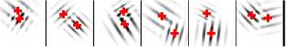
(a)

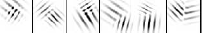
(b)

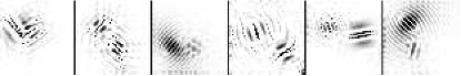
(c)

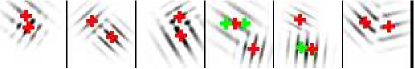
(d)

Figure 4: (a) Some randomly generated images by combination of two Gabor functions. Centers of Gabor functions are marked with a red plus sign. (b) Non-sparse approximation of images of subfigure (a) with SIKL algorithm. Since the learned Gabor functions are present at all support vector locations, they cannot be assigned to any specific location. (c) An image of support vector pixels in which the darkness of each pixel is proportional to the magnitude of its support vector coefficient. (d) Approximation of images of subfigure (a) obtained by learning a sparse Gabor-based representation. Red/Green plus signs correspond to the centers of the Gabor functions contributing positively/negatively in the learned sparse representation.

7 Conclusion

In this paper, we exploited the fact that a practical form of Gabor functions is also a positive-definite kernel to find an image representation based on Gabor functions. This representation is learned by the stabilized infinite kernel learning regression algorithm that had been previously proposed by Ghiasi-Shirazi [18]. The obtained representation has the weakness that the learned Gabor kernels are not localized and are present at all pixels. We proposed a sparse representation algorithm based on LASSO and showed that in simple cases it can recover the underlying generating Gabor functions of images. As an application of our method, we proposed an algorithm for automatic learning of parameters of Gabor filters in the task of face recognition. Our experiments on CMU-PIE and Extended Yale B datasets confirm the usefulness of the proposed algorithm in automatic learning of Gabor filters.

8 Acknowledgment

The author wishes to express appreciation to Research Deputy of Ferdowsi University of Mashhad for supporting this project by grant No.: 2/38449. The author thanks Chuan-Xian Ren for providing him with the code of the MOST algorithm [36] and the processed versions of CMU-PIE and Extended Yale B datasets. The author also thanks his colleagues, Ahad Harati and Ehsan Fazl-Ersi for their valuable comments.

Appendix A Gabor functions as positive definite kernels

Two dimensional Gabor functions have been studied in depth by Lee [24]. He starts from a general form of Gabor functions that consists of 8 parameters as follows:

$$\begin{aligned} \Psi&(x,y;x_{0},y_{0},\xi_{0},\nu_{0},\rho,\theta,\sigma,\beta)=\\ &\frac{1}{\sqrt{\pi\sigma\beta}}e^{-\left(\frac{\left((x-x_{0})cos{\theta}+(y-y_{0})sin{\theta}\right)^{2}}{2\sigma^{2}}+\frac{\left(-(x-x_{0})sin{\theta}+(y-y_{0})cos{\theta}\right)^{2}}{2\beta^{2}}\right)}\\ &\times e^{i(\xi_{0}(x-x_{0})+\nu_{0}(y-y_{0})+\rho)}\end{aligned}$$ (28)

where the pair $(x_{0},y_{0})$ is the center of the filter in spatial domain, the parameters $\beta,\sigma,\theta$ determine an elliptical Gaussian, the parameters $\xi_{0},\nu_{0}$ are the horizontal and vertical frequencies, and $\rho$ is the phase parameter. He then simplifies the form of Gabor functions by setting $\rho=0$. Note that, even after setting $\rho=0$, the above form of Gabor functions is unwantedly too general and includes both Gaussian filters (when frequency parameters are zero) and sinusoidal waves (when $\sigma,\beta\to\infty$). Considering the biological observations reported about the biological visual cells, Lee [24] reduces the number of parameters one by one until he arrives at a form with only two parameters. Similar two parameter forms for Gabor functions have been used by other researchers[27, 26, 36, 20, 38]. All of these forms are special cases of Eq. (28) with $\rho=0$. We now prove that Gabor functions are positive definite kernels.

Proposition 1.

The complex-valued Gabor function $k([x,y],[x^{\prime},y^{\prime}])$ defined by the following equation is a positive definite kernel:

$$\begin{aligned} k(&[x,y],[x^{\prime},y^{\prime}])=\\ &\frac{1}{\sqrt{\pi\sigma\beta}}e^{-\left(\frac{\left((x-x^{\prime})cos{\theta}+(y-y^{\prime})sin{\theta}\right)^{2}}{2\sigma^{2}}+\frac{\left(-(x-x^{\prime})sin{\theta}+(y-y^{\prime})cos{\theta}\right)^{2}}{2\beta^{2}}\right)}\\ &\times e^{i(\xi_{0}(x-x^{\prime})+\nu_{0}(y-y^{\prime}))}.\end{aligned}$$ (29)

Proof.

Since the leading coefficient $\frac{1}{\sqrt{\pi\sigma\beta}}$ is positive and the class of positive definite kernels is closed under multiplication, it is enough to prove that the following functions are positive definite:

$$\begin{aligned} k_{1}(&[x,y],[x^{\prime},y^{\prime}])=\\ &\exp{\left(-\frac{\left((x-x^{\prime})cos{\theta}+(y-y^{\prime})sin{\theta}\right)^{2}}{2\sigma^{2}}\right)}\\ k_{2}(&[x,y],[x^{\prime},y^{\prime}])=\\ &\exp{\left(-\frac{\left(-(x-x^{\prime})sin{\theta}+(y-y^{\prime})cos{\theta}\right)^{2}}{2\beta^{2}}\right)}\\ k_{3}&([x,y],[x^{\prime},y^{\prime}])=e^{i(\xi_{0}(x-x^{\prime})+\nu_{0}(y-y^{\prime}))}.\end{aligned}$$ (30)

The functions $k_{1}$ and $k_{2}$ are positive definite since they are Gaussian functions with general covariance matrices. Considering the fact that any function of the form $k(z,z^{\prime})=f(z)\bar{f(z^{\prime})}$ is positive definite[41], positive definiteness of $k_{3}$ follows from the following equation:

$$\begin{aligned} k_{3}&([x,y],[x^{\prime},y^{\prime}])=e^{i(\xi_{0}x+\nu_{0}y)}e^{-i(\xi_{0}x^{\prime}+\nu_{0}y^{\prime})}\end{aligned}$$ (31)

.

Corollary 1.

Any real-valued Gabor function expressible in the following form is a positive definite kernel.

$$\begin{aligned} k(&[x,y],[x^{\prime},y^{\prime}])=\\ &\frac{1}{\sqrt{\pi\sigma\beta}}e^{-\left(\frac{\left((x-x^{\prime})cos{\theta}+(y-y^{\prime})sin{\theta}\right)^{2}}{2\sigma^{2}}+\frac{\left(-(x-x^{\prime})sin{\theta}+(y-y^{\prime})cos{\theta}\right)^{2}}{2\beta^{2}}\right)}\\ &\times cos(\xi_{0}(x-x^{\prime})+\nu_{0}(y-y^{\prime}))\end{aligned}$$ (32)

.

Proof.

This follows from the fact that the real part of a complex-valued positive definite kernel function is a real-valued positive definite kernel [see 39, page 31].

References

- Argyriou et al. [2005] A. Argyriou, C.A. Micchelli, and M. Pontil. Learning convex combinations of continuously parameterized basic kernels. In Proceedings of the 18th Conference on Learning Theory, volume 18, pages 338–352, 2005.
- Argyriou et al. [2006] A. Argyriou, R. Hauser, C.A. Micchelli, and M. Pontil. A DC-programming algorithm for kernel selection. In Proceedings of the International Conference on Machine Learning, volume 23, pages 338–352, Pittsburgh, PA, 2006.
- Bach et al. [2004] F.R. Bach, G.R.G. Lanckriet, and M.I. Jordan. Multiple kernel learning, conic duality, and the SMO algorithm. In Proceedings of the 21st International Conference on Machine Learning, volume 21, pages 41–48, Banff, Canada, 2004. Omnipress.
- Baker et al. [2003] S Baker, T Sim, and M Bsat. The cmu pose, illumination, and expression database. IEEE Transaction on Pattern Analysis and Machine Intelligence, 25(12):1615–1618, 2003.
- Bishop [1995] Christopher M Bishop. Neural networks for pattern recognition. Oxford university press, 1995.
- Bucak et al. [2014] Serhat S Bucak, Rong Jin, and Anil K Jain. Multiple kernel learning for visual object recognition: A review. IEEE Transactions on Pattern Analysis and Machine Intelligence, 36(7):1354–1369, 2014.
- Cament et al. [2015] L.A. Cament, F.J. Galdames, K.W. Bowyer, and C.A. Perez. Face recognition under pose variation with local gabor features enhanced by active shape and statistical models. Pattern Recognition, 48(11):3371–3384, 2015. doi: 10.1016/j.patcog.2015.05.017.
- Chang and Morgan [2014] Shuo-Yiin Chang and Nelson Morgan. Robust cnn-based speech recognition with gabor filter kernels. In INTERSPEECH, pages 905–909, 2014.
- Cristianini and Shawe-Taylor [2000] N. Cristianini and J. Shawe-Taylor. An Introduction to Support Vector Machines. Cambridge University Press, 2000.
- Daugman [1980] John G Daugman. Two-dimensional spectral analysis of cortical receptive field profiles. Vision research, 20(10):847–856, 1980.
- Daugman [1985] John G Daugman. Uncertainty relation for resolution in space, spatial frequency, and orientation optimized by two-dimensional visual cortical filters. JOSA A, 2(7):1160–1169, 1985.
- Erhan et al. [2010] Dumitru Erhan, Yoshua Bengio, Aaron Courville, Pierre-Antoine Manzagol, Pascal Vincent, and Samy Bengio. Why does unsupervised pre-training help deep learning? Journal of Machine Learning Research, 11(Feb):625–660, 2010.
- Fischer et al. [2006] Sylvain Fischer, Gabriel Cristóbal, and Rafael Redondo. Sparse overcomplete gabor wavelet representation based on local competitions. IEEE Transactions on Image Processing, 15(2):265–272, 2006.
- Gehler and Nowozin [2008] P. V. Gehler and S. Nowozin. Infinite kernel learning. In Proceedings of the NIPS 2008 Workshop on ”Kernel Learning: Automatic Selection of Optimal Kernels”, pages 1–4, 2008.
- Genton [2001] M.G. Genton. Classes of kernels for machine learning: A statistics perspective. Journal of Machine Learning Research, 2:299–312, 2001.
- Georghiades et al. [2001] Athinodoros S. Georghiades, Peter N. Belhumeur, and David J. Kriegman. From few to many: Illumination cone models for face recognition under variable lighting and pose. IEEE transactions on pattern analysis and machine intelligence, 23(6):643–660, 2001.
- Ghiasi-Shirazi et al. [2010] Kamaledin Ghiasi-Shirazi, Reza Safabakhsh, and Mostafa Shamsi. Learning translation invariant kernels for classification. Journal of Machine Learning Research, 11(Apr):1353–1390, 2010.
- Ghiasi-Shirazi [2011] Sayed Kamaledin Ghiasi-Shirazi. Learning kernel functions based on a stabilized convex combination model. PhD thesis, Department of Computer Engineering and Information Technology, Amirkabir University of Technology (Tehran Polytechnic), 2011. (In Farsi language).
- Gu et al. [2012] W. Gu, C. Xiang, Y.V. Venkatesh, D. Huang, and H. Lin. Facial expression recognition using radial encoding of local gabor features and classifier synthesis. Pattern Recognition, 45(1):80–91, 2012. doi: 10.1016/j.patcog.2011.05.006.
- Haghighat et al. [2013] Mohammad Haghighat, Saman Zonouz, and Mohamed Abdel-Mottaleb. Identification using encrypted biometrics. In International Conference on Computer Analysis of Images and Patterns, pages 440–448. Springer, 2013.
- Kloft et al. [2011] Marius Kloft, Ulf Brefeld, Sören Sonnenburg, and Alexander Zien. Lp-norm multiple kernel learning. Journal of Machine Learning Research, 12(Mar):953–997, 2011.
- Lanckriet et al. [2004] G.R.G. Lanckriet, N. Cristianini, P. Bartlett, L. El Ghaoui, and M.I. Jordan. Learning the kernel matrix with semidefinite programming. Journal of Machine Learning Research, 5:27–72, 2004.
- Lee [2015] J.-C. Lee. Copy-move image forgery detection based on gabor magnitude. Journal of Visual Communication and Image Representation, 31:320–334, 2015. doi: 10.1016/j.jvcir.2015.07.007.
- Lee [1996] Tai Sing Lee. Image representation using 2d gabor wavelets. IEEE Transactions on pattern analysis and machine intelligence, 18(10):959–971, 1996.
- Li et al. [2017] C. Li, Y. Huang, and L. Zhu. Color texture image retrieval based on gaussian copula models of gabor wavelets. Pattern Recognition, 64:118–129, 2017. doi: 10.1016/j.patcog.2016.10.030.
- Liu [2004] Chengjun Liu. Gabor-based kernel pca with fractional power polynomial models for face recognition. IEEE transactions on pattern analysis and machine intelligence, 26(5):572–581, 2004.
- Liu and Wechsler [2002] Chengjun Liu and Harry Wechsler. Gabor feature based classification using the enhanced fisher linear discriminant model for face recognition. IEEE Transactions on Image processing, 11(4):467–476, 2002.
- Liu and Wechsler [2003] Chengjun Liu and Harry Wechsler. Independent component analysis of gabor features for face recognition. IEEE transactions on Neural Networks, 14(4):919–928, 2003.
- Marĉelja [1980] S Marĉelja. Mathematical description of the responses of simple cortical cells. JOSA, 70(11):1297–1300, 1980.
- Micchelli and Pontil [2005] C.A. Micchelli and M. Pontil. Learning the kernel function via regularization. Journal of Machine Learning Research, 6:1099–1125, 2005.
- Özöğür-Akyüz and Weber [2010a] S Özöğür-Akyüz and G-W Weber. Infinite kernel learning via infinite and semi-infinite programming. Optimisation Methods & Software, 25(6):937–970, 2010a.
- Özöğür-Akyüz and Weber [2010b] S Özöğür-Akyüz and G-W Weber. On numerical optimization theory of infinite kernel learning. Journal of Global Optimization, 48(2):215–239, 2010b.
- Pan and Ruan [2008] X. Pan and Q.-Q. Ruan. Palmprint recognition using gabor feature-based (2d)2pca. Neurocomputing, 71(13-15):3032–3036, 2008. doi: 10.1016/j.neucom.2007.12.030.
- Pan and Ruan [2009] X. Pan and Q.-Q. Ruan. Palmprint recognition using gabor-based local invariant features. Neurocomputing, 72(7-9):2040–2045, 2009. doi: 10.1016/j.neucom.2008.11.019.
- Rakotomamonjy et al. [2008] A. Rakotomamonjy, F.R. Bach, S. Canu, and V. Grandvalet. SimpleMKL. Journal of Machine Learning Research, 9:2491–2521, 2008.
- Ren et al. [2014] Chuan-Xian Ren, Dao-Qing Dai, Xiao-Xin Li, and Zhao-Rong Lai. Band-reweighed gabor kernel embedding for face image representation and recognition. IEEE Transactions on Image Processing, 23(2):725–740, 2014.
- Rudin [1987] W. Rudin. Real & Complex Analysis, 3rd edition. McGraw-Hill, New York, 1987.
- Saremi et al. [2013] Saeed Saremi, Terrence J Sejnowski, and Tatyana O Sharpee. Double-gabor filters are independent components of small translation-invariant image patches. Neural computation, 25(4):922–939, 2013.
- Schölkopf and Smola [2002] B. Schölkopf and A. Smola. Learning with Kernels- Support Vector Machines, Regularization, Optimization and Beyond. MIT Press, Cambridge, MA, 2002.
- Serre et al. [2007] Thomas Serre, Lior Wolf, Stanley Bileschi, Maximilian Riesenhuber, and Tomaso Poggio. Robust object recognition with cortex-like mechanisms. IEEE transactions on pattern analysis and machine intelligence, 29(3):411–426, 2007.
- Shawe-Taylor and Cristianini [2004] J. Shawe-Taylor and N. Cristianini. Kernel Methods for Pattern Analysis. Cambridge University Press, 2004.
- Sonnenburg et al. [2006] S. Sonnenburg, G. Rätsch, C. Schafer, and B. Schölkopf. Large scale multiple kernel learning. Journal of Machine Learning Research, 7:1531–1567, 2006.
- Tibshirani [1996] Robert Tibshirani. Regression shrinkage and selection via the lasso. Journal of the Royal Statistical Society. Series B (Methodological), pages 267–288, 1996.
- Xu et al. [2009] Zenglin Xu, Rong Jin, Irwin King, and Michael Lyu. An extended level method for efficient multiple kernel learning. In Advances in neural information processing systems, pages 1825–1832, 2009.
- Yang et al. [2013] Meng Yang, Lei Zhang, Simon CK Shiu, and David Zhang. Gabor feature based robust representation and classification for face recognition with gabor occlusion dictionary. Pattern Recognition, 46(7):1865–1878, 2013.
- Zhang et al. [2014] L. Zhang, D. Tjondronegoro, and V. Chandran. Random gabor based templates for facial expression recognition in images with facial occlusion. Neurocomputing, 145:451–464, 2014. doi: 10.1016/j.neucom.2014.05.008.
- Zhang and Liu [2013] Y. Zhang and C. Liu. Gabor feature-based face recognition on product gamma manifold via region weighting. Neurocomputing, 117:1–11, 2013. doi: 10.1016/j.neucom.2012.12.053.