B stars seen at high resolution by XMM-Newton

We report on the properties of 11 early B stars observed with gratings on board XMM-Newton and Chandra, thereby doubling the number of B stars analysed at high resolution. The spectra typically appear soft, with temperatures of 0.2–0.6 keV, and moderately bright ($\log[L_{\rm X}/L_{\rm BOL}]\sim-7$) with lower values for later type stars. In line with previous studies, we also find an absence of circumstellar absorption, negligible line broadening, no line shift, and formation radii in the range 2 – 7 R_⋆. From the X-ray brightnesses, we derived the hot mass-loss rate for each of our targets and compared these values to predictions or values derived in the optical domain: in some cases, the hot fraction of the wind can be non-negligible. The derived X-ray abundances were compared to values obtained from the optical data, with a fair agreement found between them. Finally, half of the sample presents temporal variations, either in the long-term, short-term, or both. In particular, HD 44743 is found to be the second example of an X-ray pulsator, and we detect a flare-like activity in the binary HD 79351, which also displays a high-energy tail and one of the brightest X-ray emissions in the sample.

1 Introduction

The advent of the first high-resolution X-ray spectrographs on board XMM-Newton and Chandra profoundly modified our understanding of high-energy phenomena. Indeed, high-resolution spectra provide a wealth of detailed information. For massive stars, the X-ray emission comes from optically thin, hot plasma; hence lines dominate the X-ray spectra. Their relative strengths closely constrain the plasma temperature and composition. The ratios between forbidden and intercombination lines of He-like ions further pinpoint where X-rays arise (Porquet et al., 2001). Finally, their line profiles provide unique information on the stellar wind, its opacity, and its velocity field (Macfarlane et al., 1991; Owocki & Cohen, 2001).

Analyses of the high-resolution spectra of O stars have revealed winds to be less opaque than initially thought and have helped constraining the properties of high-energy interactions (e.g. colliding winds in binaries and magnetically confined winds in strongly magnetic objects). However, many fewer B stars were observed at high resolution. To further advance the understanding of X-rays associated with early B stars, we present in this paper the X-ray observations of 11 additional targets, thereby doubling the number of such stars observed at high resolution. Section 2 presents the selection of targets, their properties, and their observations. Sections 3 and 4 report our analyses of spectra and light curves, respectively, while Sect. 5 summarises and concludes this paper.

2 Target selection and observations

Performing a spectroscopic X-ray survey of early-type B stars at high resolution can only be carried out if the X-ray emission is sufficiently bright; this is the case even with XMM-Newton,  which is the most sensitive facility currently available. A target selection was therefore performed with the ROSAT All-Sky Survey (RASS): objects with RASS count rates larger than 0.1 cts s^-1 yield usable RGS spectra within relatively short exposure times; still, for the great majority of the observations, these exposure times are greater than 20 ks. There are 20 such B stars in the catalogue of Berghöfer et al. (1996), but one (HD 152234) actually is an O+O binary (for an analysis of its XMM-Newton low-resolution data, see Sana et al., 2006) and the high-resolution spectra of 8 stars have been previously analysed. These include the strongly magnetic stars HD 205021 ($\beta$ Cep, B1III+B6–8+A2.5V; Favata et al., 2009) and HD 149438 ($\tau$ Sco, B0.2V; Cohen et al., 2003; Mewe et al., 2003; Waldron & Cassinelli, 2007; Zhekov & Palla, 2007), as well as HD 122451 ($\beta$ Cen, B1III; Raassen et al., 2005), HD 116658 (Spica, B1III-IV; Zhekov & Palla, 2007; Miller, 2007), HD 111123 ($\beta$ Cru, B0.5III+B2V+PMS; Zhekov & Palla, 2007; Waldron & Cassinelli, 2007; Cohen et al., 2008), HD 93030 ($\theta$ Car, B0.2V; Nazé & Rauw, 2008), HD 37128 ($\epsilon$ Ori, B0I; Waldron & Cassinelli, 2007; Zhekov & Palla, 2007), and the peculiar Be star HD 5394 ($\gamma$ Cas; Smith et al. 2004; Lopes de Oliveira et al. 2010; Smith et al. 2012). This leaves 11 stars, which we analyse here using observations taken by XMM-Newton or Chandra (see Table 1 for the observing log). This table also presents the main properties of the targets. Amongst these targets, four are known binaries (HD 63922, HD 79351, HD 144217, and HD 158926; see Table 1) while two are known $\beta$ Cephei pulsators (HD 44743 and HD 158926; see Sect. 4 for more details). Six targets were also searched for the presence of magnetic fields. HD 36512 (Bagnulo et al., 2006; Grunhut et al., 2017), HD 36960 (Bagnulo et al., 2006; Bychkov et al., 2009), HD 79351 (Hubrig et al., 2007), and HD158926 (Bychkov et al., 2009) seem non-magnetic while HD 44743 and HD 52089 may present very weak fields ($<$100 G; Fossati et al., 2015; Neiner et al., 2017); no strongly magnetic star is thus known in our sample. Finally, there is no Be star amongst them, hence none can belong to the class of peculiar, X-ray bright $\gamma$-Cas objects. We thus refrain from comparing our targets to such objects in the following, especially since their X-ray emission has a completely different origin than for normal B stars (for a review, see Smith et al., 2016). We make comparisons, however, with the published analyses of the 7 other B stars.

Table 1: Journal of the observations and physical properties of the sample stars.

Target name	Sp. type	$d$	log($L_{\rm BOL}/L_{\odot}$)	$R_{\star}$	$T_{\rm eff}$	$N^{ism}_{\rm H}$	ObsID (Rev)	Obs. mode	PI	Start date	Flare?	Duration
		(pc)		($R_{\odot}$)	(K)	($10^{22}$ cm-2)						(ks)
HD 34816 ($\lambda$ Lep)	B0.5 V [1] *	261	4.22	4.7	30400	1.66e-2	0690200601 (2415)	ff+thick	Nazé	2013-02-15@07:41:26	N	26.5
HD 35468 ($\gamma$ Ori)	B2 IV–III [2] *	77	3.87	6.4	21250	1.82e-3	0690680501 (2342)	ff+thick	Waldron	2012-09-22@19:27:17	Y	42.0
HD 36512 ($\upsilon$ Ori)	B0 V [1] *	877	5.21	12.1	33400	1.95e-2	0690200201 (2326)	ff+thick	Nazé	2012-08-22@02:46:15	Y	20.2
HD 36960	B0.7 V [1] *	495	4.58	7.8	29000	2.24e-2	0690200501 (2433)	ff+thick	Nazé	2013-03-23@08:57:52	Y	28.2
HD 38771 ($\kappa$ Ori)	B0.5 Ia [3]	198	4.72	12.5	24800	3.39e-2	9940	ACIS-S	Waldron	2008-12-26@23:50:00		234.2
							10846	+HETG,		2008-12-30@02:53:17
							9939	faint		2009-01-03@03:00:24
							10839			2009-01-05@18:25:49
HD 44743 ($\beta$ CMa)	B1 II–III [4]	151	4.41	8.8	24700	2.00e-4	0503500101 (1509)	ff+thick	Waldron	2008-03-06@15:33:36	Y	10.6
							0761090101 (2814)	ff+thick	Oskinova	2015-04-21@06:44:53	Y	78.0
HD 52089 ($\epsilon$ CMa)	B1.5 II [4]	124	4.35	9.9	22500	1.00e-4	0069750101 (0234)	ff(MOS)/sw(pn)+thick	Cohen	2001-03-19@12:05:51	Y	31.2
HD 63922 (P Pup)	B0.2 III+? [1,5] *	505	4.95	10.4	31200	6.71e-2	0720390601 (2552)	ff+thick	Nazé	2013-11-15@02:11:45	N	46.5
HD 79351 (a Car)	B2.5 V+? [6,7] *	137	3.60	5.8	19150	6.04e-2	0690200701 (2393)	ff+thick	Nazé	2013-01-02@00:12:30	N	47.1
HD 144217 ($\beta^{1}$ Sco)	B0.5IV-V+B1.5V [8] *	124	4.44	6.1	30400	1.37e-1	0690200301 (2425)	ff+thick	Nazé	2013-03-06@16:04:28	N	26.6
HD 158926 ($\lambda$ Sco)	B1.5 IV+ (DA.79
	or PMS)+B [9,10] *	175	4.73	15.3	22500	2.51e-3	0690200101 (2424)	ff+thick	Nazé	2013-03-04@15:37:29	N	17.8

2.1 XMM-Newton

The XMM-Newton data were reduced with the Science Analysis Software (SAS) v16.0.0 using calibration files available in Spring 2016 and following the recommendations of the XMM-Newton team.

After the initial pipeline processing, the European Photon Imaging Camera (EPIC) observations were filtered to keep only the best-quality data (pattern 0–12 for MOS and 0–4 for pn). Light curves for events beyond 10 keV were calculated for the full cameras and, whenever background flares were detected, the corresponding time intervals were discarded; we used thresholds of 0.2 cts s^-1 for MOS, 0.5 cts s^-1 for pn in full-frame mode and 0.04 cts s^-1 for pn in small window mode. We extracted EPIC spectra using the task especget in circular regions of 50″ radius for MOS and 35″ for pn (to avoid CCD gaps) centred on the Simbad positions of the targets except for HD 36960 and HD 144217, for which the radii were reduced to 25″ and 7.5″  respectively, owing to the presence of neighbouring sources. Dedicated Ancillary Response File (ARF) and Redistribution Matrix File (RMF) response matrices, which are used to calibrate the flux and energy axes, respectively, were also calculated by this task. We grouped EPIC spectra with specgroup to obtain an oversampling factor of five and to ensure that a minimum signal-to-noise ratio of 3 (i.e. a minimum of 10 counts) was reached in each spectral bin of the background-corrected spectra; unreliable bins below 0.25 keV were discarded. We extracted EPIC light curves in the same regions as the spectra, for time bins of 100 s and 1 ks, and in the 0.3–10.0 keV energy band. These light curves were further processed by the task epiclccorr, which corrects for the loss of photons due to vignetting, off-axis angle, or other problems such as bad pixels. In addition, to avoid very large errors, we discarded bins displaying effective exposure time lower than 50% of the time bin length.

The Reflection Grating Spectrometer (RGS) data were also locally processed using the initial SAS pipeline. As for EPIC data, a flare filtering was then applied (using a threshold of 0.1 cts s^-1). For HD 36960 and HD 144217, close companions exist at a distance of 0.14–0.62’ and 0.2’, respectively, perpendicular to the dispersion axis. The extraction region was thus reduced to 45% and 50% of the PSF radius, respectively, to avoid contamination. Furthermore, the background was extracted after excluding regions within 98% of the PSF size from the source and neighbours. Dedicated response files were calculated for both orders and both RGS instruments and were subsequently attached to the source spectra for analysis. The two RGS datasets of HD 44743 were combined using rgscombine. For individual line analyses, no grouping and no background were considered (the local background around the lines was simply fitted using a flat power law). For global fits, background spectra were considered and a grouping was performed to reach at least 10 cts per bin and to get emissions of each He-like ($fir$) triplet in a single bin. The latter step is needed because global spectral fitting does not take into account the possible depopulation of the upper level of the $f$-line in triplets in favour of the upper levels of the $i$-lines.

2.2 Chandra

The Chandra data of HD 38771 were reprocessed locally using CIAO 4.9 and CALDB 4.7.3. Since all Chandra data were taken within 10 days, orders +1 and –1 were added and the four exposures combined using combine_grating_spectra to get the final HEG and MEG spectra. For each exposure, 0th order spectra of the source were also extracted in a circle of 2.5″ radius around its Simbad position, while the associated background spectra were extracted in the surrounding annulus with radii 2.5 and 7.4″. Dedicated response matrices were calculated using the task specextract, and the individual spectra and matrices were then combined using the task combine_spectra to get a single spectrum for HD 38771. The resulting HEG, MEG, and 0th order spectra were grouped in the same way as the XMM-Newton spectra. For each exposure, light curves were extracted considering the same regions as the spectra, for time bins of 100 s and 1 ks, and in the 0.3–10.0 keV energy band.

3 Spectra

We performed two types of fitting: individual analyses of the lines and global analyses. All these analyses were performed within Xspec v 12.9.0i.

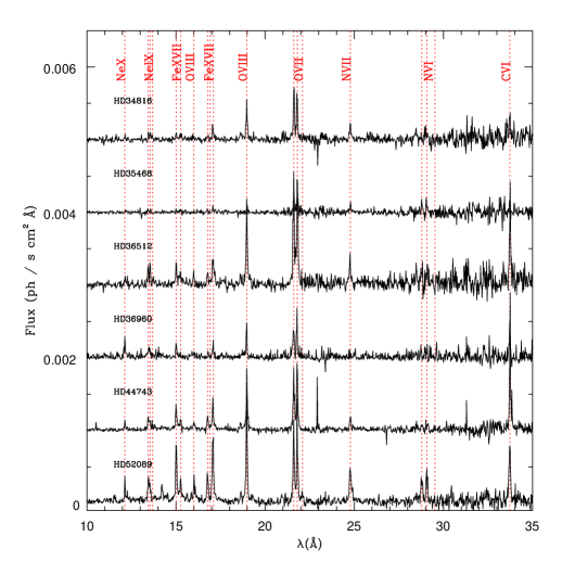
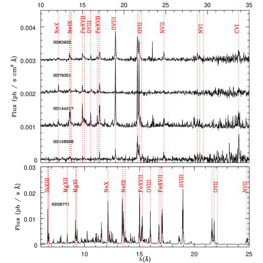
Figure 1: RGS and MEG spectra of our targets with the main lines identified and their position indicated by the dotted lines.

3.1 Line fits

Figure 1 shows the high-resolution spectra of our targets. Lines from H-like and He-like ions of C, N, O, Ne, Mg, and Si, along with lines from ionised Fe, are readily detected, demonstrating the thermal nature of the X-ray emissions. In general, the triplet from He-like ions appear stronger than Ly$\alpha$ lines, as expected for late-type massive stars (Walborn et al., 2009), but we find no clear, systematic dependence with the spectral types of our targets.

An examination of the line profiles reveals no obvious asymmetry, hence we decided to fit them by simple Gaussian profiles. We relied on Cash statistics and therefore used unbinned spectra without background correction. We only fitted the lines that were sufficiently intense to provide a meaningful fit. In case of doublets (the two components of Lyman lines of H-like ions) or triplets (the $fir$ components of He-like ions), the individual components were forced to share the same velocity and the same width. Furthermore, the flux ratios between the two Lyman components and the flux ratios between the two $i$ lines of Si and Mg were fixed to the theoretical ratios in ATOMDB. The derived line properties are listed in Table 2 with 1$\sigma$ errors determined using the error command under Xspec. Whenever the fitted width was reaching a null value, a second fitting was performed with the width fixed to zero, and Table 2 provides the results of this second fitting.

Table 2: Results of the individual line fitting by Gaussians.

	HD 34816	HD 35468	HD 36512	HD 36960	HD 38771	HD 44743	HD 52089	HD 63922	HD 79351	HD 144217	HD 158926
He-like triplets
Si xiii $\lambda$6.648,6.685,6.688,6.740Å
$v$ (km s-1)					136$\pm$90
$FWHM$ (km s-1)					1201$\pm$182
$F_{r}$					2.72$\pm$0.33
$F_{i}$					0.62$\pm$0.19
$F_{f}$					1.29$\pm$0.23
$f/i$					2.08$\pm$0.74
$(f+i)/r$					0.70$\pm$0.14
$T_{fir}$ (keV)					1.30$\pm$0.81
Mg xi $\lambda$9.169,9.228,9.231,9.314Å
$v$ (km s-1)					–34$\pm$57
$FWHM$ (km s-1)					1132$\pm$108
$F_{r}$					5.45$\pm$0.55
$F_{i}$					3.00$\pm$0.48
$F_{f}$					2.87$\pm$0.45
$f/i$					0.96$\pm$0.21
$(f+i)/r$					1.08$\pm$0.16
$T_{fir}$ (keV)					0.25$\pm$0.08
$R_{fir}$ ($R_{\star}$)					2.38$\pm$0.44
Ne ix $\lambda$13.447,13.553,13.699Å
$v$ (km s-1)			–160$\pm$67		–54$\pm$44	–95$\pm$110	24$\pm$130	–54$\pm$109		–37$\pm$86
$FWHM$ (km s-1)			0 (fixed)		1310$\pm$71	732$\pm$309	830$\pm$291	369$\pm$441		0 (fixed)
$F_{r}$			22.9$\pm$4.5		50.1$\pm$3.0	17.3$\pm$2.4	33.8$\pm$4.6	17.5$\pm$2.5		38.0$\pm$7.4
$F_{i}$			26.7$\pm$4.7		31.7$\pm$2.9	11.2$\pm$2.2	19.5$\pm$4.2	12.1$\pm$2.4		41.5$\pm$8.4
$F_{f}$			6.53$\pm$3.38		7.97$\pm$1.62	3.28$\pm$1.47	0.46$\pm$2.59	5.56$\pm$1.89		4.36$\pm$4.56
O vii $\lambda$21.602,21.804,22.098Å
$v$ (km s-1)	1$\pm$146	142$\pm$111	0$\pm$57	–254$\pm$98	–2$\pm$47	–31$\pm$31	0$\pm$60	79$\pm$61		–135$\pm$61	0$\pm$108
$FWHM$ (km s-1)	0 (fixed)	0 (fixed)	361$\pm$353	313$\pm$406	1353$\pm$80	426$\pm$198	0 (fixed)	1033$\pm$144		0 (fixed)	845$\pm$391
$F_{r}$	66.0$\pm$8.3	18.7$\pm$4.1	161$\pm$17	44.1$\pm$9.9	300$\pm$27	84.5$\pm$6.8	107$\pm$8	102$\pm$8		204$\pm$19	82.9$\pm$10.0
$F_{i}$	73.1$\pm$8.6	28.8$\pm$4.7	175$\pm$20	53.8$\pm$10.3	238$\pm$24	107$\pm$7	117$\pm$9	90.6$\pm$7.9		210$\pm$20	57.2$\pm$9.9
$F_{f}$	2.87$\pm$3.95	0 (fixed)	3.08$\pm$6.03	0.20$\pm$4.65	25.2$\pm$10.3	0.$\pm$0.73	6.80$\pm$3.95	1.18$\pm$3.13		4.59$\pm$6.96	8.65$\pm$5.94
$f/i$	0.04$\pm$0.05	0 (fixed)	0.02$\pm$0.03	0.0$\pm$0.09	0.11$\pm$0.04	0.000$\pm$0.007	0.06$\pm$0.03	0.01$\pm$0.03		0.02$\pm$0.03	0.15$\pm$0.11
$(f+i)/r$	1.15$\pm$0.20	1.55$\pm$0.42	1.11$\pm$0.17	1.22$\pm$0.38	0.88$\pm$0.12	1.26$\pm$0.13	1.16$\pm$0.13	0.90$\pm$0.11		1.05$\pm$0.14	0.79$\pm$0.17
$T_{fir}$ (keV)	0.09$\pm$0.05	¡0.09	0.10$\pm$0.03	0.09$\pm$0.08	0.22$\pm$0.08	¡0.09	0.09$\pm$0.03	0.18$\pm$0.06		0.12$\pm$0.05	0.26$\pm$0.18
$R_{fir}$ ($R_{\star}$)	¡10.1		¡8.3	¡9.8	7.4$\pm$2.3	¡2.1	4.5$\pm$2.4	¡6.9		¡7.6	7.3$\pm$6.5
N vi $\lambda$28.787,29.084,29.535Å
$v$ (km s-1)							–127$\pm$76
$FWHM$ (km s-1)							685$\pm$182
$F_{r}$							42.8$\pm$5.9
$F_{i}$							49.3$\pm$9.2
$F_{f}$							0.0$\pm$3.1
$f/i$							0.00$\pm$0.06
$(f+i)/r$							1.15$\pm$0.28
$T_{fir}$ (keV)							0.09$\pm$0.08
$R_{fir}$ ($R_{\star}$)							¡3.7

Table 2: Continued

	HD 34816	HD 35468	HD 36512	HD 36960	HD 38771	HD 44743	HD 52089	HD 63922	HD 79351	HD 144217	HD 158926
Lyman doublets
Mg xii $\lambda$8.419,8.425Å
$v$ (km s-1)					–222$\pm$200
$FWHM$ (km s-1)					1046$\pm$475
$F$					0.91$\pm$0.21
He-to-H ratio					12.5$\pm$3.1
$T_{He/H}$ (keV)					0.42$\pm$0.02
Ne x $\lambda$12.132,12.137Å
$v$ (km s-1)				1$\pm$314	–72$\pm$43	1$\pm$147	4$\pm$192		283$\pm$80
$FWHM$ (km s-1)				1111$\pm$836	1037$\pm$93	0 (fixed)	0 (fixed)		0 (fixed)
$F$				24.9$\pm$4.1	19.4$\pm$1.3	13.4$\pm$1.7	25.8$\pm$3.1		18.5$\pm$2.7
O viii Ly$\alpha$ $\lambda$18.967,18.973Å
$v$ (km s-1)	–2$\pm$69	144$\pm$379	0$\pm$31	–292$\pm$194	–144$\pm$36	0$\pm$27	–33$\pm$33	27$\pm$53	112$\pm$120	–87$\pm$41	–127$\pm$156
$FWHM$ (km s-1)	583$\pm$322	1750$\pm$1750	0 (fixed)	0 (fixed)	1267$\pm$69	0 (fixed)	283$\pm$247	709$\pm$190	0 (fixed)	0 (fixed)	760$\pm$759
$F$	57.1$\pm$4.2	12.3$\pm$2.2	126$\pm$8	42.2$\pm$5.4	261$\pm$11	97.0$\pm$3.2	159$\pm$5	109$\pm$5	22.4$\pm$3.2	218$\pm$13	32.4$\pm$4.2
He-to-H ratio	2.49$\pm$0.28	3.85$\pm$0.85	2.69$\pm$0.27	2.33$\pm$0.47	2.16$\pm$0.17	1.97$\pm$0.12	1.45$\pm$0.09	1.78$\pm$0.14		1.92$\pm$0.17	4.59$\pm$0.76
$T_{He/H}$ (keV)	0.193$\pm$0.004	0.18$\pm$0.01	0.189$\pm$0.004	0.19$\pm$0.01	0.198$\pm$0.004	0.207$\pm$0.004	0.22$\pm$0.01	0.202$\pm$0.005		0.189$\pm$0.004	0.168$\pm$0.004
O viii Ly$\beta$ $\lambda$16.006,16.007Å
$v$ (km s-1)			–228$\pm$152		–130$\pm$145	0$\pm$279	160$\pm$60	84$\pm$206		–171$\pm$171
$FWHM$ (km s-1)			0 (fixed)		1296$\pm$159	1087$\pm$429	0 (fixed)	933$\pm$602		0 (fixed)
$F$			14.7$\pm$3.6		34.0$\pm$3.3	11.3$\pm$1.8	26.0$\pm$3.4	14.4$\pm$2.5		34.0$\pm$4.5
N vii $\lambda$24.779,24.785Å
$v$ (km s-1)	–73$\pm$133		–299$\pm$107		92$\pm$131	2$\pm$123	85$\pm$83	–4$\pm$118
$FWHM$ (km s-1)	439$\pm$495		0 (fixed)		1838$\pm$233	0 (fixed)	1264$\pm$254	729$\pm$535
$F$	23.4$\pm$4.8		37.2$\pm$8.2		158$\pm$15	19.5$\pm$2.7	72.0$\pm$5.9	24.8$\pm$4.4
He-to-H ratio							1.28$\pm$0.19
$T_{He/H}$ (keV)							0.15$\pm$0.01
C vi $\lambda$33.734,33.740Å
$v$ (km s-1)			64$\pm$86			0$\pm$60	–122$\pm$49				122$\pm$91
$FWHM$ (km s-1)			470$\pm$469			268$\pm$267	328$\pm$328				0 (fixed)
$F$			127$\pm$17			84.1$\pm$8.1	91.1$\pm$8.4				79.9$\pm$13.6
Fe xvii $\lambda$15.014,15.261Å
$v$ (km s-1)			1$\pm$50		–115$\pm$36	9$\pm$49	0$\pm$56	188$\pm$130	0$\pm$65	104$\pm$166
$FWHM$ (km s-1)			0 (fixed)		1192$\pm$81	707$\pm$185	0 (fixed)	927$\pm$477	0 (fixed)	1385$\pm$482
$F$			38.7$\pm$5.2		96.2$\pm$4.4	51.6$\pm$2.5	112$\pm$5	33.0$\pm$3.4	26.4$\pm$2.8	84.5$\pm$8.2
Fe xvii $\lambda$16.780,17.051,17.096Å
$v$ (km s-1)			–373$\pm$154		–585$\pm$42	–474$\pm$58	–602$\pm$26	–490$\pm$86	–614$\pm$147	–665$\pm$56
$FWHM$ (km s-1)			937$\pm$632		989$\pm$90	0 (fixed)	0 (fixed)	504$\pm$504	0 (fixed)	0 (fixed)
$F_{16.780}$			17.1$\pm$3.9		40.2$\pm$4.2	18.8$\pm$1.9	40.3$\pm$3.5	8.28$\pm$2.07	5.42$\pm$2.03	21.6$\pm$4.9
$F_{both\,17}$			54.1$\pm$8.1		107$\pm$6	49.4$\pm$3.0	115$\pm$5	33.7$\pm$3.3	27.7$\pm$3.0	79.7$\pm$8.1

We compared the results obtained for the different lines for each target, taking the errors into account but we detected no significant ($>3\sigma$) and coherent line shifts for any of them. There are systematic blueshifts for the iron lines near 17Å for all targets, which remain unexplained and are probably not real. Excluding these blueshifts, we find that 59% of measurements lie within $\pm 1\sigma$ of zero, 83% lie within $\pm 2\sigma$, and 97% lie within $\pm 3\sigma$; these measurements match well the normal distribution centred on zero. Our targets hence display no line shifts. Similarly, the line widths appear overall negligible compared to the resolution for all targets except HD 38771, for which $FWHM\sim 1250$ km s^-1, which is a value close to the wind terminal velocity (Crowther et al., 2006; Searle et al., 2008). While other stars were observed using the RGS, which has a poorer spectral resolution than HEG/MEG, it should be noted that $FWHM$ larger than 1000 km s^-1 would have been detected, considering the errors and instrumental broadening. The X-ray lines thus generally appear quite narrow, confirming the results found for other B stars (e.g. Waldron & Cassinelli, 2007; Cohen et al., 2008; Favata et al., 2009).

We now turn to the line ratios: $(f+i)/r$ in He-like triplets and flux ratios between He-like and H-like lines are indicators of temperature while $\mathcal{R}=f/i$ is a probe of the formation radius of the X-ray emission. Correcting for the energy-dependent interstellar absorption is unnecessary for ratios involving the closely spaced $fir$ lines, but such a correction needs to be performed for the He-to-H-like flux ratios since the lines are more distant in this case. However, since our targets are nearby, their interstellar absorptions are small (Table 1), hence these corrections are of very limited amplitude.

As in Nazé et al. (2012), we used the ATOMDB, although with the newer version 3.0.8, to compute the expected ratios He-to-H-like flux ratios and $(f+i)/r$ ratios as a function of temperatures, and compared them to the observed values (see results in Table 2). The derived temperatures, typically $\log(T)\sim 6.35$, are in line with the lowest ones found in global fits (see next section) and are also comparable to temperatures observed in normal B stars (e.g. Waldron & Cassinelli, 2007; Zhekov & Palla, 2007, see also further below).

The negligible $f$ lines indicate that the emission from He-like triplets arises close to a source of UV, i.e. close to the stellar photosphere (e.g. Porquet et al. 2001). In fact, for massive stars, $\mathcal{R}=f/i=\mathcal{R}_{0}/(1+\phi/\phi_{\rm C})$. The $\mathcal{R}_{0}$ values were derived from ATOMDB calculations, and taken at the temperature indicated by the $(f+i)/r$ ratio (see above and Table 2). The $\phi_{\rm C}$ values were taken from Blumenthal et al. (1972). Finally, we used TLUSTY spectra (Lanz & Hubeny, 2003, 2007) in the UV domain with solar abundances to get the stellar fluxes in the velocity interval [–2000; 0] km s^-1 near the rest wavelengths of the 2³S₁ $\rightarrow$ 2³P_1,2 transition (for a similar approach, see Leutenegger et al. 2006). We consider TLUSTY models with the closest temperatures to the ones listed in Table 1 and the closest surface gravities predicted by Nieva (2013) for the different spectral types of non-supergiant stars – for HD 38771, HD 44743, and HD 52089, the surface gravities derived by Touhami et al. (2010) and Fossati et al. (2015) were considered. A microturbulence velocity of $\xi$=10 km s^-1, which is a value adapted to our target types (e.g. Hunter et al. 2009), was considered, unless models with the required temperatures and surface gravities were not available within the TLUSTY grid associated to $\xi$=10 km s^-1 (i.e. for HD 35468, HD 44743, HD 52089, and HD 158926). In this case, TLUSTY models with $\xi$=2 km s^-1 were taken into account. We performed tests to check the consistency of our choice: using these two microturbulence velocities resulted in similar formation radii, within error bars, for an effective temperature of 22000 K and a surface gravity of 3.00 dex. Since these UV fluxes are diluted for calculating the $\phi$ values, which can be represented by the multiplication by the dilution factor $W(r)=0.5\,\{1-[1-(R_{\star}/r)^{2}]^{1/2}\}$, the $\mathcal{R}$ ratios constrain the position of the emitting plasma (see $R_{fir}$ in Table 2). Note that UV TLUSTY spectra only cover the 900 – 3200 $\AA$ wavelength range, which therefore excludes the analysis of the Si xiii triplet lines, hence $R_{fir}$ is not indicated in that case, but this concerned only HD 38771 (and its $f/i$ ratio is very similar to that reported for HD 37128, HD 111123, or HD 149438 by Waldron & Cassinelli 2007). Focusing on the formation radii derived from O vii lines (since they are available for all but one star), values ranging from $\sim$ 2 to $\sim$ 8 $R_{\star}$ are found. This is in good agreement with values determined for the same lines for the studied B stars mentioned in Sect. 2: for HD 205021, Favata et al. (2009) derived a formation radius in the range $\simeq$ 3 – 5 $R_{\star}$; for HD 122451, Raassen et al. (2005) estimated a formation radius $\lesssim$ 5.7 $R_{\star}$; Nazé & Rauw (2008) gave a formation radius ¡ 20 $R_{\star}$ for HD 93030; Miller (2007) derived a formation radius in the range 5 – 8 $R_{\star}$ for HD 116658; Mewe et al. (2003) estimated the formation radius of HD 149438 to be $\lesssim$ 10 $R_{\star}$; for HD 37128, Waldron & Cassinelli (2007) provided a formation radius of 10.2$\pm$2.6 $R_{\star}$.

3.2 Global fits

Having both low-resolution, broadband spectra (EPIC, ACIS-S 0th order) and high-resolution, narrower band spectra (RGS, HEG/MEG) allows us to investigate the full X-ray spectra in detail, deriving not only temperatures and absorptions, but also abundances. However, caution must be taken since abundances may vary wildly when all parameters are relaxed in one step. Therefore, we performed global fits in several steps. First, we fitted the low-resolution spectra with absorbed thermal emission models with fixed solar abundances (Asplund et al., 2009). One thermal component was never sufficient to achieve a good fit, but two components were usually adequate, except for HD 36960, HD 79351, and HD 144217, for which three components were needed to fit a high-energy tail. Fits with absorption in addition to the interstellar one were tried, but either the additional absorbing column reached a null value or the $\chi^{2}$ was worse than without such a column. This absence of (detectable) local absorption is usual for B stars (Nazé et al., 2011; Rauw et al., 2015) and for the final fits we therefore considered only the interstellar contributions (see Table 1 for their values). Second, we fitted the high-resolution spectra with the same thermal models, but we fixed the temperatures while releasing abundances. The abundance of an element is only allowed to vary if lines of that element are clearly observed (and measured, see Table 2). In the third step, the temperatures were released again for fitting the high-resolution spectra. Finally, in the fourth step, a simultaneous fitting of both low-resolution and high-resolution spectra was performed with the same model as in the third step. The final results are provided in Table 3. The abundances found in the last two steps are similar, but they sometimes differ from those found in the second step, indicating that the formal error bars might actually be underestimated.

Table 3: Results of the global fitting using models of the type $tbabs(ism)\times\sum vapec_{i}$.

	HD 34816	HD 35468	HD 36512	HD 36960	HD 38771∗	HD 44743	HD 52089	HD 63922	HD 79351	HD 144217	HD 158926
$kT_{1}$	0.186$\pm$0.004	0.172$\pm$0.004	0.116$\pm$0.008	0.081$\pm$0.001	0.215$\pm$0.010	0.197$\pm$0.001	0.199$\pm$0.002	0.190$\pm$0.002	0.223$\pm$0.016	0.188$\pm$0.003	0.174$\pm$0.006
$norm_{1}$	8.63$\pm$0.42	2.91$\pm$0.10	19.8$\pm$3.7	13.6$\pm$0.78	46.5$\pm$4.3	7.66$\pm$0.28	9.93$\pm$0.40	13.3$\pm$0.5	4.07$\pm$0.23	27.6$\pm$1.21	5.37$\pm$0.40
$kT_{2}$	0.41$\pm$0.07	0.59$\pm$0.03	0.291$\pm$0.004	0.459$\pm$0.015	0.52$\pm$0.02	0.558$\pm$0.006	0.579$\pm$0.004	0.488$\pm$0.017	0.74$\pm$0.02	0.481$\pm$0.019	0.48$\pm$0.06
$norm_{2}$	0.46$\pm$0.30	0.19$\pm$0.02	7.00$\pm$0.55	1.20$\pm$0.04	7.30$\pm$0.82	1.91$\pm$0.05	5.78$\pm$0.13	1.78$\pm$0.13	3.73$\pm$0.09	4.18$\pm$0.35	0.43$\pm$0.09
$kT_{3}$				2.50$\pm$0.08					1.60$\pm$0.03	4.4$\pm$6.2
$norm_{3}$				2.85$\pm$0.07					3.73$\pm$0.09	0.32$\pm$0.10
$\chi_{\nu}^{2}$ (dof)	1.39(454)	1.04(463)	1.31 (476)	1.35 (463)	1.08 (521)	1.54 (1414)	1.44 (1139)	1.21 (798)	1.40 (1020)	1.20 (377)	1.12 (312)
$A_{C}$			0.61$\pm$0.16			1.69$\pm$0.16	1.26$\pm$0.13				1.61$\pm$0.35
$A_{N}$	1.07$\pm$0.13		1.03$\pm$0.17		1.05$\pm$0.33	1.27$\pm$0.09	2.28$\pm$0.15	1.21$\pm$0.11
$A_{O}$	0.54$\pm$0.03	0.45$\pm$0.03	0.97$\pm$0.11	2.74$\pm$0.15	0.33$\pm$0.03	0.78$\pm$0.03	0.76$\pm$0.03	0.69$\pm$0.03	0.34$\pm$0.03	0.78$\pm$0.04	0.74$\pm$0.07
$A_{N}/A_{C}$			1.69$\pm$0.52			0.75$\pm$0.09	1.81$\pm$0.22
$A_{N}/A_{O}$	1.98$\pm$0.26		1.06$\pm$0.21		3.18$\pm$1.04	1.62$\pm$0.13	3.00$\pm$0.23	1.75$\pm$0.18
$A_{Ne}$			1.41$\pm$0.12	5.40$\pm$0.32	0.65$\pm$0.07	1.79$\pm$0.08	1.67$\pm$0.07	1.29$\pm$0.06	1.99$\pm$0.42	1.73$\pm$0.10
$A_{Fe}$			0.83$\pm$0.06		0.40$\pm$0.04	1.00$\pm$0.03	0.85$\pm$0.02	0.87$\pm$0.04	0.78$\pm$0.04	0.93$\pm$0.06
$A_{O}/A_{Fe}$			1.17$\pm$0.16		0.83$\pm$0.11	0.78$\pm$0.04	0.89$\pm$0.04	0.79$\pm$0.05	0.44$\pm$0.04	0.84$\pm$0.07
$F^{\rm obs}_{\rm X}$	0.42$\pm$0.02	0.135$\pm$0.003	1.08$\pm$0.03	0.83$\pm$0.06	2.10$\pm$0.06	0.926$\pm$0.005	1.80$\pm$0.01	0.788$\pm$0.006	1.037$\pm$0.007	1.47$\pm$0.02	0.343$\pm$0.010
log($L_{\rm X}/L_{\rm BOL}$)	$-7.24\pm 0.02$	$-8.48\pm 0.01$	$-6.77\pm 0.01$	$-6.76\pm 0.03$	$-7.26\pm 0.01$	$-7.597\pm 0.002$	$-7.421\pm 0.002$	$-7.044\pm 0.003$	$-6.767\pm 0.003$	$-7.38\pm 0.01$	$-8.21\pm 0.01$
eq. ROSAT c.r.	0.134	0.095	0.397	0.176	0.326	0.341	0.537	0.091	0.102	0.142	0.178

In general, the X-ray spectra appear very soft and the associated temperatures are low, i.e. 0.2–0.6 keV, in line with results from Raassen et al. (2005); Zhekov & Palla (2007); Nazé & Rauw (2008); Gorski & Ignace (2010) for optically bright, nearby B stars observed at high resolution in X-rays. However, in large surveys relying on low-resolution X-ray spectra, many B stars present higher temperatures (Nazé, 2009; Nazé et al., 2011), although the contamination by companions or magnetically confined winds cannot be excluded in such cases. In our sample, only three targets appear harder with a hotter component, i.e. HD 36960, HD 79351, and HD 144217. The last two are binaries and we may suspect that this plays a role in their properties. However, only longer observations including full monitoring throughout the orbital period, would be able to reveal the exact origin of the hard X-rays, which could be emitted by the companion or result from an interaction with it. For HD 36960, however, there is no obvious reason for such a hardness: it is not a known binary or magnetic object. Further investigation is thus needed to clarify this issue.

The X-ray luminosities of massive stars are generally compared to their bolometric luminosities (see penultimate line of Table 3). For single and non-magnetic O-type stars in clusters, the ratio $\log(L_{\rm X}/L_{\rm BOL})$ is close to $-7$ with a dispersion of about 0.2 dex (e.g. Nazé et al., 2011). The situation appears more complex for early B stars. Surveys show a large scatter with ratios between –8 and –6 and the X-ray emission often appears at a constant flux level for the (rather few) detected cases (Berghöfer et al., 1996; Nazé et al., 2011, 2014; Rauw et al., 2015); again, contamination of the X-ray emission by companions cannot be excluded. Furthermore, while magnetic O stars systematically appear brighter than their non-magnetic counterparts, this is not the case of magnetic B stars ($\log{[L_{\rm X}/L_{\rm BOL}]}\sim-7.6$ for the faintest case in Fig. 4 and Table 7 of Nazé et al., 2014), which further blurs the picture. However, our sample is rather clean in this respect, as the chosen B stars are nearby and not strongly magnetic (see Sect. 2). Our earliest B-type stars (B0–0.7) display ratios between –6.8 and –7.4, in line with the O-star relationship. This confirms previous results for such objects (Rauw et al., 2015, and references therein). Four of the five latest B-type stars (B1–2.5) have ratios $<-7.4$, confirming the lower level of intrinsic X-ray emission of such (non-magnetic) stars found in ROSAT data (Cohen et al., 1997) and attributed to their weakest stellar winds. However, the last star, HD 79351, appears overluminous. This can probably be explained by its binarity; in this context, it is interesting to note that a flare occurred during the observation of this star (see next section).

In massive stars, X-rays are linked to stellar winds. The amount of X-ray emission can therefore be used to estimate the amount of mass loss heated to high temperatures. This is important information since, in the tenuous winds of B stars and late O stars, cooling times are long and hence the plasma remains hot once heated. Estimating mass-loss rates from optical/UV diagnostics may thus lead to underestimations. This was clearly demonstrated by Huenemoerder et al. (2012) for the late O star HD 38666 (see also a similar discussion for HD 111123 in Cohen et al. 2008). We have used the best-fit normalisation factors (Table 3) to calculate the total emission measures $EM$s (since $norm=10^{-14}\,EM/[4\,\pi\,d^{2}]$), summing those of individual components (Table 4). These values were converted into rates of hot mass loss considering Eq. 1 of Huenemoerder et al. (2012) and its equivalent for constant velocity on p. 1868 of Cohen et al. (2008, correcting by the different stellar radii of our targets). This was carried out considering terminal wind velocities of 500, 1000, and 1500 km s^-1 and the formation radius derived for O vii lines (Table 2). The derived range of values are provided in Table 4. We also computed mass-loss rates from the formulae of Vink et al. (2001, listed in Table 4), using the temperature and bolometric luminosities of our targets listed in Table 1, along with typical masses for the spectral types of our targets, taken from Cox (2002). Finally, mass-loss estimates derived from the analysis of optical spectra are also provided in Table 4, when available. Comparing all these values, we find that our targets fall into two categories. The hot plasma constitutes a small (or even negligible) part of the wind for HD 36512, HD 38771, HD 44743, HD 63922, and HD 158926, or about half of the sample. For the other stars, the hot plasma appears as the dominant component of the circumstellar environment, as in HD 38666 (Huenemoerder et al., 2012). In examining which stellar properties could justify this dichotomy, we find variable stars (see next section) and binaries in both categories; hence variability or multiplicity are not specific characteristics of stellar winds dominated by hot plasma. However, the three stars displaying a very hot component in their X-ray spectrum all belong to the second category, i.e. stars whose winds appear to be dominated by hot plasma. For such stars, the $EM$ may not perfectly reflect the intrinsic X-ray emission as there may be contamination by X-rays arising in a companion, in an interaction with it, or a still unknown phenomenon (see above). Further investigation is thus needed to ascertain that most of their wind truly is hot. In any case, our analysis suggests that some B stars have their winds in the X-ray emitting regime, such that using only optical/UV data could lead to underestimation of their actual mass-loss rate. We caution, however, that this result is preliminary, as detailed analysis of the optical/UV spectra are often not available for those stars.

Table 4: Derived mass loss from optical studies and estimates, from different prescriptions, of the hot mass loss derived with our X-ray data.

Target name	$\log(\dot{M}_{\rm literature})$	$\log(\dot{M}_{\rm Vink+01})$		$EM$	$\log(\dot{M}_{\rm Huenemoerder+12})$	$\log(\dot{M}_{\rm Cohen+08})$
	(M⊙ yr-1)	(M⊙ yr-1)		(1052 cm-3)	(M⊙ yr-1)	(M⊙ yr-1)
		Low $T_{\rm eff}$	High $T_{\rm eff}$
HD 34816			$-$8.50$\pm$0.06	74.1$\pm$4.2	¡–8.1 to ¡–7.6	¡–8.0 to ¡–7.6
HD 35468		$-$8.33$\pm$0.09		2.20$\pm$0.07	–10.0 to –8.4 a	–9.3 to –8.4 a
HD 36512			$-$6.22$\pm$0.06	2466$\pm$344	¡–7.2 to ¡–6.7	¡–7.1 to ¡–6.6
HD 36960			$-$7.79$\pm$0.07	159$\pm$23	¡–7.8 to ¡–7.3	¡–7.8 to ¡–7.3
HD 38771	$-$6.05 [1], $-5.92_{-0.07}^{+0.11}$ [2]	$-$6.80$\pm$0.08	$-$8.01$\pm$0.07	252$\pm$21	–7.7 to –7.2	–7.6 to –7.2
HD 44743		$-$7.33$\pm$0.08	$-$8.55$\pm$0.08	26.1$\pm$0.8	¡–8.6 to ¡–8.2	¡–8.5 to ¡–8.0
HD 52089	$-9$ [3],$-8$ [4]	$-$7.53$\pm$0.08		28.9$\pm$0.8	–8.3 to –7.8	–8.3 to –7.8
HD 63922			$-$6.93$\pm$0.06	460$\pm$16	¡–7.6 to ¡–7.1	¡–7.6 to ¡–7.1
HD 79351		$-$8.71$\pm$0.10		25.9$\pm$0.6	–9.5 to –7.9 a	–8.7 to –7.8 a
HD 144217			$-$8.04$\pm$0.06	59.1$\pm$2.3	¡–8.1 to ¡–7.7	¡–8.1 to ¡–7.6
HD 158926		$-$6.50$\pm$0.08		19.8$\pm$1.5	–8.2 to –7.7	–8.1 to –7.7

The abundances of our sample stars derived from our X-ray fits are listed in Table 3 and those determined in optical studies from the literature are listed in Table 5. Figure 2 provides a graphical comparison for the main elements (N, O, and Fe) for the stars in common. Except for the high O enrichment derived in X-rays for HD 36960, which is not confirmed in the optical domain, the agreement between the derived abundances is fair (generally well within 3$\sigma$). Indeed, the formal fit errors are known to be smaller than the actual fit errors (e.g. de Plaa et al. 2017). An example of disagreement can also be found in the subsolar abundances found by Cohen et al. (2008) and Zhekov & Palla (2007) for HD 111123: even though they analysed the same dataset, the Zhekov & Palla (2007) abundances of O, Ne, and Mg are a factor of two smaller than those of Cohen et al. (2008); the origin of this discrepancy is unknown. We also note disagreements between optical studies, for example for HD 38771 or HD 52089, showing that improvements are required there too. In any case, not many comparisons between X-ray and optical abundances can be found in the literature. For HD 205021, Favata et al. (2009) derived O, Si, and Fe abundances that are depleted compared to photospheric abundances. Nazé & Rauw (2008) confirmed the depletion in C and O of HD 93030 as well as its enrichment in N reported in the optical domain by Hubrig et al. (2008). In fact, X-ray determinations would benefit from higher S/N data; for example, the X-ray abundances of HD 66811, derived from very high-quality spectra, could be better constrained (Hervé et al., 2013).

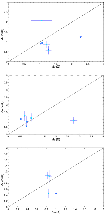
Figure 2: Comparison between our N (upper panel), O (middle panel), and Fe (lower panel) abundance estimates and recent literature values obtained by optical studies. Circles, triangles, diamonds, squares, and star symbols represent values obtained by Nieva & Przybilla (2012), Venn et al. (2002), Valdes et al. (2004), Searle et al. (2008), and Morel et al. (2006, 2008), respectively.

Table 5: Stellar abundances from optical studies.

	HD 34816	HD 35468	HD 36512	HD 36960	HD 38771
$A_{C}$	0.68 [1], 0.89$\pm$0.15 [2]	0.71 [3], 0.74 [1]	0.83$\pm$0.28 [2], 0.85$\pm$0.31 [7], 0.89$\pm$0.31 [6]	0.74$\pm$0.18 [9], 0.83$\pm$0.20 [2]	0.11 [10], 0.20 [11]
$A_{N}$	0.68 [1], 0.95$\pm$0.35 [2]	1.82 [3], 2.00 [1]	0.89$\pm$0.31 [6], 0.91$\pm$0.36 [2], 1.00$\pm$0.26 [7]	0.76$\pm$0.16 [9], 0.78$\pm$0.22 [2]	0.35$\pm$0.13, 2.69$\pm$0.92 [10], 2.09 [11]
$A_{O}$	1.04$\pm$0.25 [2], 1.15 [1]		1.05$\pm$0.34 [8], 1.06$\pm$0.41 [6], 1.15$\pm$0.27 [2]	0.95$\pm$0.21 [2], 1.07$\pm$0.21 [9]	1.10 [11], 1.29$\pm$0.38 [10]
$A_{N}/A_{C}$	1.00 [1], 1.07$\pm$0.43 [2]	2.56 [3], 2.70 [1]	1.10$\pm$0.57 [2], 1.00$\pm$0.49 [6], 1.18$\pm$0.53 [7]	0.94$\pm$0.35 [2], 1.03$\pm$0.33 [9]	3.18$\pm$1.18;24.5$\pm$8.4 [10], 10.45 [11]
$A_{N}/A_{O}$	0.59 [1], 0.91$\pm$0.40 [2]		0.84$\pm$0.44 [6], 0.79$\pm$0.36 [2]	0.71$\pm$0.20 [9], 0.82$\pm$0.39 [2]	0.27$\pm$0.13;2.09$\pm$0.94 [10], 1.90 [11]
$A_{Ne}$	1.77$\pm$0.16 [2]	1.12$\pm$0.26 [4]	1.52$\pm$0.43 [2], 1.70$\pm$0.55 [7]	1.59$\pm$0.54 [2]
$A_{Fe}$	1.10$\pm$0.20 [2]	0.83 [5]	1.07$\pm$0.12 [2], 1.12$\pm$0.12 [7]	0.96$\pm$0.22 [2]
$A_{O}/A_{Fe}$	0.95$\pm$0.28 [2]		1.07$\pm$0.28 [2]	0.99$\pm$0.32 [2]
$A_{Mg}$					0.40 [10]
$A_{Si}$					0.45 [10]
	HD 44743	HD 52089	HD 63922
$A_{C}$	0.54$\pm$0.15 [12], 0.60 [1], 0.63 [3], 0.78$\pm$0.20 [14]	0.46$\pm$0.14 [12], 0.74$\pm$0.15 [14]	0.74$\pm$0.15 [2]
$A_{N}$	0.58$\pm$0.20 [12], 0.76 [1], 0.79 [3], 0.83$\pm$0.24 [14]	0.81 [15], 1.26$\pm$0.43 [12], 2.15$\pm$0.42 [14]	0.87$\pm$0.19 [2]
$A_{O}$	0.85$\pm$0.37 [12], 1.15 [1], 1.23 [3], 1.10$\pm$0.28 [14]	0.56$\pm$0.24 [12], 1.02$\pm$0.30 [14]	1.26$\pm$0.32 [2]
$A_{N}/A_{C}$	1.07$\pm$0.48 [12], 1.27 [1], 1.25 [3], 1.06$\pm$0.41 [14]	2.74$\pm$1.25 [12], 2.91$\pm$0.82 [14]	1.18$\pm$0.35 [2]
$A_{N}/A_{O}$	0.68$\pm$0.38 [12], 0.66 [1], 0.64 [3], 0.75$\pm$0.29 [14]	2.25$\pm$1.23 [12], 2.11$\pm$0.74 [14]	0.69$\pm$0.23 [2]
$A_{Ne}$	0.91$\pm$0.34 [4]	0.85$\pm$0.24 [4]	1.37$\pm$0.39 [2]
$A_{Fe}$	0.47$\pm$0.21 [13]	0.46$\pm$0.16 [12]	1.03$\pm$0.21 [2]
$A_{O}/A_{Fe}$		1.22$\pm$0.67 [12]	1.22$\pm$0.40 [2]

4 Light curves

We finally examined the temporal evolution of the X-ray brightnesses of our targets. The light curves in the 0.3–10. keV energy band are shown in Fig. 3. We first performed $\chi^{2}$ tests for three different null hypotheses (constancy, linear variation, and quadratic variation). The improvement of the $\chi^{2}$ when increasing the number of parameters in the model (e.g. linear trend versus constancy) was also determined by means of Snedecor F tests (nested models; see Sect. 12.2.5 in Lindgren, 1976). As threshold for significance, we used 1% and we considered that a threshold of 10% indicates only marginal evidence. This yields the following results.

Two stars are clearly compatible with constancy, i.e. HD 34816 and HD 38771. For the latter, only the ACIS-S light curve with 1ks bins could be analysed, as there are not enough counts in each bin for a meaningful $\chi^{2}$ test of the 100s-binned light curves. We also analysed the light curves of each Chandra exposure with the appropriate CIAO tool, and the variability index was found to be zero (definitely not variable) for ObsID 9939, 10839, and 10846, and 2 (probably not variable) for ObsID 9940, which confirms the $\chi^{2}$ results. We also tested the combination of the four individual light curves using $\chi^{2}$ tests with the same null result as for individual light curves.

Four stars reveal marginal variability (i.e. presence of trends and/or rejection of constancy at the 1–10% level), i.e. HD 35468, HD 44743, HD 63922, and HD 144217. HD 35468 is detected to be variable for the MOS2 light curves, but this star is only marginally variable in pn data and appears to be compatible with constancy in MOS1 data. For HD 44743, trends provide better fits for pn data in Rev. 1509 and for MOS1 and pn data for Rev. 2814. A marginal variability is further detected for all instruments in Rev. 2814, and when the two datasets are combined. The 100s-bin light curves of HD 144217 are better fitted by trends.

Five stars exhibit a clear variability (significance level ¡1%), i.e. HD 36512, HD 36960, HD 52089, HD 79351, and HD 158926. HD 36512 is detected to be variable for the 100s-bin pn light curve, and a trend provides a clearly better fit than a constant for MOS2 and pn. HD 36960 appears significantly variable for all instruments, with trends – especially parabolic trends – always providing better fits. Indeed, the light curve presents a large oscillation with maxima at the beginning and end of the exposure and a minimum in between. This change in brightness is only marginally accompanied by a change in hardness (see Fig. 4), however. HD 52089 appears variable in pn data and a trend provides a clearly better fit than a constant. HD 79351 appears significantly variable for all instruments. Indeed, the light curve steedily increases at first, then slightly decreases, and finally presents a flare-like activity. Furthermore, when it brightens, HD 79351 also becomes harder (see Fig. 4). HD 158926 is detected to be significantly variable for all instruments when considering 100s bins, with trends providing a better fit to pn data.

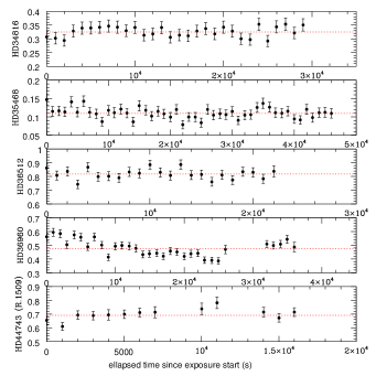
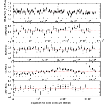
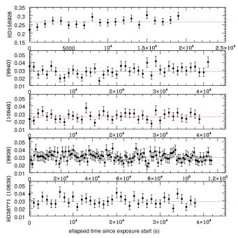
Figure 3: Light curves in units cts s^-1 from low-resolution data (EPIC-pn, ACIS-S 0th order) for the different targets in the 0.3–10.0 keV energy band and with 1ks bins. The weighted average is indicated with the dotted red line.

Figure 4: Hardness ratios as a function of the count rates, in the 0.3–10.0 keV energy band, and in units cts s^-1, for four clearly variable sources (for EPIC-pn and for 1ks bins). The hardness ratios are defined as the ratios between count rates in the 1.0–10.0 keV and 0.3–1.0 keV energy bands. The correlation coefficients amount to 40% for HD 36960, -9% for HD 52089, 81% for HD 79351, and 5% for HD 158926.

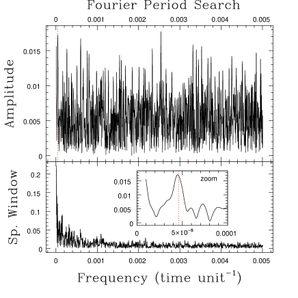
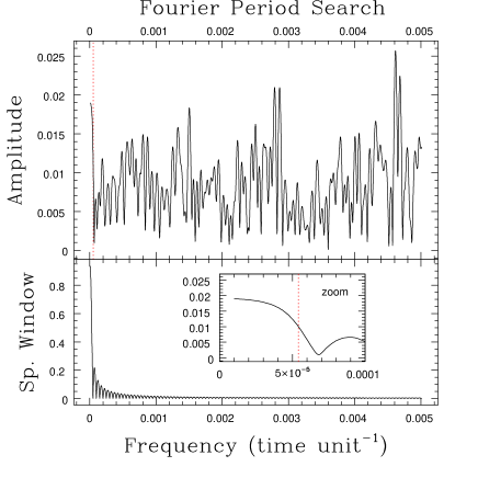
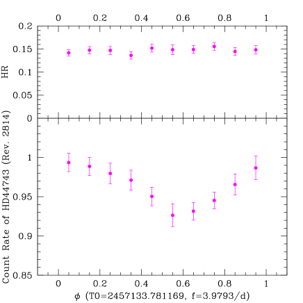
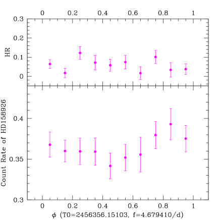
Figure 5: Top: Periodograms based on the pn light curves with 100s bins of HD 44743 (left, for Rev. 2814) and HD 158926 (right), along with their associated spectral window. An inset provides a zoom on the lowest frequencies with the $\beta$ Cephei pulsation frequencies shown by the red dotted lines. Bottom: Light curves of HD 44743 (left, for Rev. 2814) and HD158926 (right) folded using their dominant $\beta$ Cephei frequency (see text).The values $T_{0}$ are arbitrary and were chosen to correspond to the start time of the XMM-Newton observations (Table 1). The count rates correspond to EPIC values (i.e. the addition of MOS1, MOS2, and pn count rates) while the hardness ratios, defined as in Fig. 4, correspond to means (i.e. $[HR({\rm MOS1})+HR({\rm MOS2})+HR({\rm pn})]/3$). The phasing was here performed on light curves with 1ks bins; the 100s-binned light curves provide similar but slightly noisier results.

Next, we applied period search algorithms (Heck et al., 1985; Graham et al., 2013) to the light curves with 100s bins, for each EPIC camera, but no peak stands out both clearly and coherently (i.e. for all instruments) from the periodograms (although see further below).

Two types of specific timescales exist for our targets: orbital periods and pulsation periods. The former are usually long compared to the exposure length (5.9 d for HD 158926, Berghöfer et al. 2000; 6.745 d for HD 79351, Buscombe & Morris 1960; 6.83 d for HD144217, Holmgren et al. 1997), hence cannot be tested with the current dataset. However, we may still examine whether binarity may explain the flare-like behaviour of HD 79351. Indeed, Buscombe & Morris (1960) derived a mass function of 0.00663565 for this system. Assuming the mass taken from Cox (2002, $\sim 10\,M_{\odot}$) for the primary star, we find a minimum mass of $\sim 0.7M_{\odot}$ for the secondary star. It may thus be a PMS star, which could have undergone a flare during the observation. Indeed, the average X-ray luminosity of HD 79351 is $\sim$3$\times$10³⁰ erg s^-1 (Table 3) and its brightness increased by less than a factor of 2 during the flare (Fig. 3), which remains compatible with PMS flaring luminosities (Güdel & Nazé, 2009). However, a better knowledge of the HD 79351 system is needed before its X-ray properties can be fully understood.

Regarding the latter timescales, it should be noted that the following two targets are known $\beta$ Cephei: HD 44743 (three closely spaced frequencies with the strongest at $f=3.9793\pm 0.0001$ d^-1; Shobbrook et al., 2006) and HD 158926 (dominant frequency at $f=4.679410\pm 0.000013$ d^-1; Uytterhoeven et al., 2004b). For HD 44743, a peak exists close to that dominant timescale in the periodogram of EPIC data taken in Rev. 2814 (top of Fig. 5). The amplitude of this peak is not very large but it is present and in fact, if the background flares are not discarded hence longer and more complete light curves are available, this peak stands out very clearly. In this context, it should be remembered that the known pulsators HD 122451 ($\beta$ Cen), HD 116658 (Spica), HD 205021 ($\beta$ Cep), and HD 160578 ($\kappa$ Sco) do not display X-ray variations linked to their pulsations (Raassen et al., 2005; Miller, 2007; Favata et al., 2009; Oskinova et al., 2015), but HD 46328 ($\xi^{1}$ CMa) does (Oskinova et al., 2014; Nazé, 2015) and $\beta$ Cru may (Cohen et al., 2008, though see refutation in Oskinova et al. 2015). Therefore, even if periodograms do not show very strong peaks at these periods, we performed a folding using these known frequencies as a last check (bottom of Fig. 5). For HD 44743, the presence of a modulation is clearly confirmed with a peak-to-peak amplitude of 14% (corresponding to five times the error on individual bins); this modulation is not accompanied by significant hardness changes, but neither did HD 46328. The case of HD 158926 appears less convincing as the changes are not coherent from one instrument to the other, and the combination of all three EPIC instruments only leads to a slight modulation (the peak-to-peak variation is only 3$\sigma$), clearly calling for confirmation before detection can be claimed.

As a final exercise, we folded our best-fit spectral models (Table 3) through the ROSAT response matrices and derived the equivalent ROSAT count rates of our targets (reported in the last line of Table 3). Comparing our results to values tabulated by Berghöfer et al. (1996), we find negligible ($<3\sigma$) differences for all but three targets; HD 35468 and HD 158926 has become fainter by a factor of two, while HD 36512 has brightened by 50%. These three stars thus appear variable on both long and short timescales. While this could probably be linked to binarity for HD 158926, there is no clear explanation for the other two. A monitoring of all three stars will then be needed to better understand their behaviour, in particular searching for a putative periodicity.

5 Discussion and conclusions

In this paper, we analysed the X-ray data of 11 early B stars. Combined with 8 other B stars previously analysed, our results provide the first X-ray luminosity-limited survey at high resolution, thereby constituting a legacy project.

In this work, we performed line-by-line fitting, global spectral fitting (with temperatures, abundances, and brightnesses as free parameters), and variability analyses.

In many ways, our results confirm previous studies. B stars typically display soft and moderately intense X-ray emissions, their X-ray lines appear rather narrow and unshifted, and the X-ray emission arises at a few stellar radii from the photospheres.

The abundances we derived are in fair agreement with those found in optical data, taking errors into account. The X-ray brightnesses could be used to evaluate the total quantity of hot material surrounding the stars. Compared to expected mass-loss rates or values derived from the analysis of optical data, we find that in half of the cases, the hot mass-loss constitutes only a small fraction of the wind.

Roughly a quarter of our sample (3/11) display a high-energy tail and roughly half of our targets (6/11) display significant variations on short or long timescales. These properties are not mutually exclusive as two targets (HD 36960 and HD 79351) combine both specificities. Three out of the four binaries present at least one of these peculiarities, which thus appear not restricted to, but more common in, binaries.

Finally, we also analysed in detail the temporal behaviour of two $\beta$ Cephei pulsators. HD 158926 presents flux changes on both short and long timescales, but they cannot be undoubtly assigned to the pulsational activity. On the contrary, HD 44743 appears marginally variable in $\chi^{2}$ tests, but folding its light curve clearly reveals coherent variations with the optical period. This makes the star the second secure case of X-ray pulsator after HD 46328.

There remains much to be done, such as longer monitoring of the variable sources and more precise estimates of the parameters (formation radii and abundances). In this context, the advent of the Advanced Telescope for High-ENergy Astrophysics/X-ray Integral Field Unit (ATHENA/X-IFU) will certainly provide higher quality high-resolution spectra of B stars, which will further advance our understanding of their X-ray properties.