Bayesian Variable Selection For Survival Data Using Inverse Moment Priors

Abstract

Efficient variable selection in high-dimensional cancer genomic studies is critical for discovering genes associated with specific cancer types and for predicting response to treatment. Censored survival data is prevalent in such studies. In this article we introduce a Bayesian variable selection procedure that uses a mixture prior composed of a point mass at zero and an inverse moment prior in conjunction with the partial likelihood defined by the Cox proportional hazard model. The procedure is implemented in the R package BVSNLP, which supports parallel computing and uses a stochastic search method to explore the model space. Bayesian model averaging is used for prediction. The proposed algorithm provides better performance than other variable selection procedures in simulation studies, and appears to provide more consistent variable selection when applied to actual genomic datasets.

1 Introduction

Recent developments in sequencing technology have made it easier to collect massive genomic datasets that can be used to study cancer and other diseases. Given such data, there is great interest in linking genomic data to patient outcomes, and in many cases such outcomes are censored survival times.

Survival times for patients generally represent either the time to death or disease progression, the time to study termination or the time until the subject is lost to follow up. In the latter cases the subject’s survival time is censored. The relation between survival times and covariates is modeled through the hazard function, which is the limiting rate of death in the interval $(t,t+\Delta t)$ as $\Delta t$ becomes small, given patient covariates. More precisely, the hazard function $h$ for patient $i$ may be defined as

$$h(t\,|\,{\bf x}_{i})=\lim\limits_{\Delta t\rightarrow 0}\frac{1}{\Delta t}P(t\leq T\leq t+\Delta t\,|\,T\geq t,{\bf x}_{i}),$$ (1)

where ${\bf x}_{i}$ is a $p$ vector of covariates thought to influence survival. We denote by ${\bf X}$ the $n\times p$ design matrix obtained by stacking $n$ patient covariate vectors. Proportional hazard models take the form

$$h(t\,|\,{\bf x}_{i})=h_{0}(t)\Phi({\bf x}_{i})$$ (2)

with an identifiability constraint of $\Phi({\bf 0})=1$. In this formula, $h_{0}(t)$ denotes the baseline hazard function. The Cox proportional hazards model (Cox, 1972) is defined by taking $\Phi({\bf x}_{i})=\exp\{{\bf x}_{i}^{T}{\bm{\beta}}\}$, leading to

$$h(t\,|\,{\bf x}_{i})=h_{0}(t)e^{{\bf x}_{i}^{T}{\bm{\beta}}}.$$ (3)

Here, ${\bm{\beta}}$ is a $p\times 1$ vector of coefficients.

An important feature of the proportional hazards model is that it yields a partial likelihood function that is independent of the baseline hazard function, $h_{0}$. For complete survival analyses, however, the baseline hazard function is necessary for predicting survival times and can be estimated nonparametrically. Further details regarding the Cox proportional hazard model may be found in Cox and Oakes (1984), Kalbfleisch and Prentice (1980) or Cox (1972).

Gene expression datasets usually contain measurements on thousands of genes collected for only hundreds of subjects. Biologically, it seems plausible that only a relatively small number of these genes contribute significantly to survival. This implies that most of the elements in the vector ${\bm{\beta}}$ are small or close to zero. The challenge is to find covariates with nonzero coefficients or, equivalently, those genes that contribute the most in determining the survival outcome.

Many common penalized likelihood methods originally introduced for linear regression have been extended to survival data. These methods include LASSO (Tibshirani et al., 1997), in which an $L_{1}$ penalty is imposed on regression coefficients. Zhang and Lu (2007) utilized adaptive LASSO methodology for time to event data, while Antoniadis et al. (2010) adopted the Dantzig selector for survival outcomes. The extension of nonconvex penalized likelihood approaches, in particular SCAD, to the Cox proportional hazard model is discussed in Fan and Li (2002). The Iterative Sure Independence Screening (ISIS) approach introduced by Fan and Lv (2008) is also extended for ultrahigh dimensional survival data in Fan et al. (2010), where it is used on Cox proportional hazard models and the SCAD penalty is employed for variable selection.

Some Bayesian approaches have also been introduced. Faraggi and Simon (1998) proposed a method based on approximating the posterior distribution of the parameters in the proportional hazard model by defining a Gaussian prior on regression coefficients. A loss function was then imposed to select a parsimonious model. A semiparametric Bayesian approach was utilized by Ibrahim et al. (1999), who employed a discrete gamma process for the baseline hazard function and a multivariate Gaussian prior for the coefficient vector. Sha et al. (2006) considered Accelerated Failure Time (AFT) models along with data augmentation to impute failure times. A mixture prior proposed by George and McCulloch (1997) was used to impose sparsity. In more recent work, Held et al. (2016) proposed the use of a $g$-prior model for the coefficient vector and employed test-based Bayes factors (Johnson, 2005) to the Cox proportional hazard models. However, this method is intended for use only when the number of covariates is less than the number of observations, that is, when $p<n$.

To our knowledge, all previous Bayesian procedures for variable selection in survival data have used local priors on model coefficients. In Bayesian hypothesis tests, local priors put a positive probability on the null value of the parameter, in this case zero, whereas nonlocal priors put zero probability on the null value. Johnson and Rossell (2010) can be consulted for more discussion on properties of local and nonlocal priors in the context of Bayesian testing. In this article we propose a Bayesian method based on a mixture prior comprised of a point mass at zero and a nonlocal prior on the regression coefficients. To handle the computational burden of implementing the resulting procedure, we employ a stochastic search method, S5 (Shin et al., 2018), which we implement in an R package BVSNLP. We also discuss a general procedure for setting the tuning parameter of the nonlocal prior.

This article is structured as follows. In Section 2 we introduce notation and discuss the modeling of the problem in a Bayesian framework. Section 3 discusses the proposed method, with details of parameter selection, model search and assessment of the accuracy of the proposed variable selection procedure. Sections 4 and 5 provide simulation and real data analyses with various predictive performance measures to demonstrate how the proposed method compares to several other competing methods. Section 6 concludes with discussion.

2 Problem Modeling

2.1 Preliminaries

Let $T_{i}$ denote the survival time and $C_{i}$ denote the censoring time for individual $i$. Each element in the observed vector of survival times, ${\bf y}$, is defined as $y_{i}=\min\{T_{i},C_{i}\}$. The status for each individual is defined as $\delta_{i}=I(T_{i}\leq C_{i})$. The status vector is represented by ${\bm{\delta}}=(\delta_{1},\delta_{2},\ldots,\delta_{n})^{T}$. We assume that the censoring mechanism is “at random,” meaning that $C_{i}$ and $T_{i}$ are conditionally independent given ${\bf x}_{i}$, where ${\bf x}_{i}\in\mathbb{R}^{p}$ are the covariates for individual $i$ and comprise the $i^{th}$ row of ${\bf X}$. The observed data is of the form $\big{\{}(y_{i},\delta_{i},{\bf x}_{i});\;i=1,2,\ldots,n\big{\}}$.

Model ${\bf k}$ is defined as $\mathbf{k}=\{k_{1},\ldots,k_{j}\}$, where $(1\leq k_{1}<\cdots<k_{j}\leq p)$, and it is assumed that $\beta_{k_{1}}\neq 0,\ldots,\beta_{k_{j}}\neq 0$ and all other elements of $\bm{\beta}$ are 0. The design matrix corresponding to model ${\bf k}$ is denoted by ${\bf X_{k}}$ and the regression vector by ${\mathbf{\bm{\beta}_{k}}}=(\beta_{k_{1}},\beta_{k_{2}},\ldots,\beta_{k_{j}})^{T}$.

Let $\mathcal{R}(t)=\{i:y_{i}\leq t\}$ represent the risk set at time $t$, the set of all individuals who are still present in the study at time $t$ and are neither dead nor censored. We assume throughout this article that the failure times are distinct. In other words, only one individual fails at a specific failure time. With this assumption and letting $\xi_{{\bf k}_{i}}=\exp\{{\bf x}_{{\bf k}_{i}}^{T}{\mathbf{\bm{\beta}_{k}}}\}$, the partial likelihood (Cox, 1972) for ${\mathbf{\bm{\beta}_{k}}}$ in model ${\bf k}$ can be written as

$$L_{p}({\mathbf{\bm{\beta}_{k}}})=\prod\limits_{i=1}^{n}\Bigg{[}\frac{\xi_{{\bf k}_{i}}}{\sum\limits_{j\in R(y_{i})}\xi_{{\bf k}_{j}}}\Bigg{]}^{\delta_{i}}.$$ (4)

Our method uses this partial likelihood as the sampling distribution in our Bayesian model selection procedure. We acknowledge that there is some information loss in (4) with respect to ${\mathbf{\bm{\beta}_{k}}}$. For instance, Basu (Ghosh, 1988) argues that partial likelihoods cannot usually be interpreted as sampling distributions. On the other hand, Berger et al. (1999) encourage the use of partial likelihoods when the nuisance parameters are marginalized out.

Sorting the observed unique survival times in ascending order and, consequently, reordering the status vector ${\bm{\delta}}$ as well as the design matrix ${\bf X}$ with respect to the ordered ${\bf y}$, the sampling distribution of ${\bf y}$ for model ${\bf k}$ can be written as

$$\pi({\bf y}\,|\,{\mathbf{\bm{\beta}_{k}}})=\prod\limits_{i=1}^{n}\Bigg{[}\frac{e^{{\bf x}_{{\bf k}_{i}}^{T}{\mathbf{\bm{\beta}_{k}}}}}{\sum\limits_{j=i}^{n}e^{{\bf x}_{{\bf k}_{j}}^{T}{\mathbf{\bm{\beta}_{k}}}}}\Bigg{]}^{\delta_{i}}.$$ (5)

A Bayesian hierarchical model can be defined in which $\pi({\bf y}\,|\,{\mathbf{\bm{\beta}_{k}}})$ in (5) represents the sampling distribution, $\pi_{\bf k}({\mathbf{\bm{\beta}_{k}}})$ is the prior of model coefficients ${\mathbf{\bm{\beta}_{k}}}$ and $P({\bf k})$ is the prior for model ${\bf k}$. Using Bayes rule, the posterior probability for model ${\bf j}$ is written as

$$P(\mathbf{j}\,|\,{\bf y})=\frac{P(\mathbf{j})m_{\mathbf{j}}({\bf y})}{\sum_{k\in\mathcal{J}}P(\mathbf{k})m_{\mathbf{k}}({\bf y})},$$ (6)

where $\mathcal{J}$ is the set of all possible models and the marginal probability of the data under model ${\bf k}$ is defined by

$$m_{\mathbf{k}}({\bf y})=\int\pi({\bf y}\,|\,{\mathbf{\bm{\beta}_{k}}})\pi_{\bf k}({\mathbf{\bm{\beta}_{k}}})d{\mathbf{\bm{\beta}_{k}}}.$$ (7)

The prior density for ${\mathbf{\bm{\beta}_{k}}}$ and the prior on the model space impact the overall performance of the selection procedure and the amount of sparsity imposed on candidate models. Note that the sampling distribution in (5) is continuous in ${\mathbf{\bm{\beta}_{k}}}$, and in Section 2.3 we define an inverse moment prior (Johnson and Rossell, 2010) on each of the coefficients in model ${\bf k}$.

2.2 Prior on Model Space

Let ${\mathbf{\bm{\gamma}_{k}}}=\{\gamma_{1},\cdots,\gamma_{p}\}$ denote a binary vector indicating which covariates are included in model ${\bf k}$. Suppose the size of model ${\bf k}$ is $k$. That is, there are $k$ nonzero indices in ${\mathbf{\bm{\gamma}_{k}}}$. The nonzero indices of ${\mathbf{\bm{\gamma}_{k}}}$ represent the indices of the nonzero elements in the coefficient vector, ${\bm{\beta}}$, which a priori are modeled as independent Bernoulli random variables with success probability $P(\gamma_{i}=1)=\theta$ for every $1\leq i\leq p$. As discussed in Scott et al. (2010), no fixed value for $\theta$ adjusts for multiplicity. As a result, it is necessary to define a prior on $\theta$, say $\pi(\theta)$. The resulting marginal probability for model ${\bf k}$ in a fully Bayesian approach may then be written as

$$p({\bf k})\propto\int\theta^{k}(1-\theta)^{p-k}\pi(\theta)d\theta.$$ (8)

A common choice for $\pi(\theta)$ is the beta distribution, $\theta\sim\text{Beta}(a,b)$, where in the special case of $a=b=1$, $\pi(\theta)$ is a uniform distribution. The marginal probability for model ${\bf k}$ derived from (8) is then equal to

$$p({\bf k})=\frac{B(a+k,b+p-k)}{B(a,b)},$$ (9)

where $B(\cdot)$ is the Beta function. A priori, the model size, $k$, thus follows a Beta-binomial distribution. By choosing $b=p-a$, the mean and variance of the selected model size $k$ is

$$\mathbb{E}(k)=a,\quad\text{Var}(k)=\frac{2p^{2}a(p-a)}{p^{3}}\approx 2a.$$ (10)

The approximation in the variance formula follow from a large $p$ and a fairly small $a$ under the sparsity assumption on the true model size. To incorporate the belief that the optimal predictive models are sparse, we recommend setting $a=1$ and $b=p-a$. The resulting prior assigns comparatively small prior probabilities to models that contain many covariates.

2.3 Product Inverse MOMent (piMOM) Prior

We impose nonlocal prior densities on the nonzero coefficients, ${\mathbf{\bm{\beta}_{k}}}$. Specifically, we assume the prior densities on the nonzero coefficients in model ${\bf k}$ take the form of a product of independent iMOM priors, or piMOM densities (Johnson and Rossell, 2012), expressible as

$$\pi({\mathbf{\bm{\beta}_{k}}}|\tau,r)=\frac{\tau^{rk/2}}{\Gamma(r/2)^{k}}\prod_{i=1}^{k}|\beta_{i}|^{-(r+1)}\exp\Big{(}-\frac{\tau}{\beta_{i}^{2}}\Big{)},\qquad r,\tau>0.$$ (11)

The hyperparameter $\tau$ represents a scale parameter that determines the dispersion of the prior around ${\bf 0}$, while $r$ determines the tail behavior of the density. These priors have two symmetric modes with Cauchy-like tails when $r=1$, and assign negligible probability to a region around zero. In comparison to local priors, this characteristic of nonlocal priors potentially leads to smaller false positive rates in selection procedures by discouraging the selection of variables with small coefficients. On the other hand, piMOM priors possess Cauchy-like tails which introduce comparatively small penalties on large coefficients. Unlike many penalized likelihood methods, large values of regression coefficients are thus not heavily penalized by these priors. As a result, they do not necessarily impose significant penalties on nonsparse models provided that the estimated coefficients in those models are not small. For these reasons piMOM priors work well as a default choice of priors on nonnegligible coefficients in variable selection problems. An example of an iMOM prior is depicted in Figure 1 for $r=1$ and $\tau=0.5$.

Another nonlocal prior that might be considered as a potential candidate for the prior densities on the nonzero coefficients in model ${\bf k}$ is the product of independent MOM priors, or the pMOM densities (Johnson and Rossell, 2012). A detailed discussion on the pMOM priors and their properties is provided in Section 3 of the LABEL:suppA (Nikooienejad et al., 2020). A simulation analysis to compare the performance of piMOM and pMOM in the selection process is also provided. For the reasons discussed there, piMOM-based procedures are more effective for variable selection in $p\gg n$ settings and, therefore, is our choice for the analyses of the simulation and real data in this article.

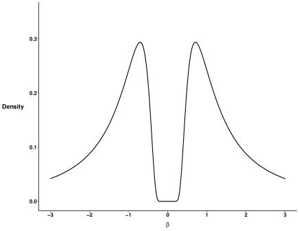
Figure 1: iMOM prior with $r=1$ and $\tau=0.5$.

3 Methods

3.1 Selection of Hyperparameters

We use the procedure described in Nikooienejad et al. (2016) to select hyperparameter values for the piMOM prior. In that method, the null distribution of the maximum likelihood estimator for ${\mathbf{\bm{\beta}_{k}}}$ (i.e., all components of ${\mathbf{\bm{\beta}_{k}}}$ are 0), obtained from randomly selected design matrices ${\bf X_{k}}$, is compared to the prior density on ${\mathbf{\bm{\beta}_{k}}}$ for various values of $(r,\tau)$. Fixing $r=1$ to achieve Cauchy-like tails, a value of $\tau$ is chosen so that the overlap between the two densities is less than a specified threshold, $1/\sqrt{p}$, and is denoted by $\tau_{1}$. It can be shown that the maximum of the iMOM prior occurs at $\pm\sqrt{\tau}$. We also allow users to input a prior parameter $\alpha$ that controls where the modes in the prior occur. This can be useful in constraining the prior density when covariates are highly correlated (resulting in an over-dispersed prior when the sampling distribution of the null MLE under the null model becomes overly broad). We then set the value of $\tau$ according to

$$\tau=\min(\tau_{1},\alpha^{2}).$$ (12)

To implement the procedure for computing $\tau_{1}$ for survival models, we generate response vectors under the null model using the procedure described by Bender et al. (2005). Survival times are sampled from a standard exponential model.

Let $\bm{t}^{s}$ and $\bm{c}^{s}$ be the vector of sampled survival times and censoring times, respectively. The sampled survival time and status for each observation is then computed as

$$y_{i}^{s}=\min\{t_{i}^{s},c_{i}^{s}\}\quad\quad\text{ and }\quad\quad\delta_{i}^{s}=I(t_{i}^{s}\leq c_{i}^{s}),$$ (13)

which comprise ${\bf y}^{s}$ and ${\bm{\delta}}^{s}$ under the null model. Using the pair $({\bf y}^{s},{\bm{\delta}}^{s})$, the MLE from a Cox model is computed. It should be noted that the asymptotic distribution of the MLE for the Cox model under the null hypothesis is $\hat{{\bm{\beta}}}\sim\mathcal{N}\big{(}{\bf 0},I(\hat{{\bm{\beta}}})\big{)}$, where $I({\bm{\beta}})$ is the information matrix of the partial likelihood function. Thus, it is appropriate to approximate the pooled estimated coefficients in that algorithm with a normal density function. When the sample size gets large, the variance of the MLE decreases and causes the overlap to become small and, consequently, small values of $\tau$ are selected.

In general, we find that $r=1$ and $\tau=0.25$ are good default values if one chooses not to run the hyperparameter selection algorithm. When $r=1$, the peaks of the iMOM prior occur at $-\sqrt{\tau}$ and $\sqrt{\tau}$. By equating $\sqrt{\tau}$ to the absolute value of the expected effect size for a given application, insight can be gained on what value of $\tau$ is appropriate. Further details regarding this algorithm can be found in Nikooienejad et al. (2016).

3.2 Computing Posterior Probability of Models

Computing the posterior probability for each model requires the marginal probability of observed survival times under each model, as shown in (6) and (7). The marginal probability is approximated using the Laplace approximation, where the regression coefficients in ${\mathbf{\bm{\beta}_{k}}}$ are integrated out. This leads to

$$m_{{\bf k}}({\bf y}_{n})=\pi({\bf y}_{n}\,|\,\hat{{\bm{\beta}}}_{\bf k})\pi(\hat{{\bm{\beta}}}_{\bf k})(2\pi)^{k/2}|G_{\hat{{\bm{\beta}}}_{\bf k}}|^{-1/2}.$$ (14)

Here, $\bm{\hat{{\bm{\beta}}}_{\bf k}}$ is the maximum a posteriori (MAP) estimate of ${\mathbf{\bm{\beta}_{k}}}$, $G_{\hat{{\bm{\beta}}}_{\bf k}}$ is the Hessian of the negative of the log posterior function,

$$g({\mathbf{\bm{\beta}_{k}}})=-\log(\pi({\bf y}\,|\,{\mathbf{\bm{\beta}_{k}}}))-\log(\pi({\mathbf{\bm{\beta}_{k}}})),$$ (15)

computed at $\bm{\hat{{\bm{\beta}}}_{\bf k}}$ and $k$ is the size of model ${\bf k}$. Finding the MAP of ${\mathbf{\bm{\beta}_{k}}}$ is equivalent to finding the minimum of $g({\mathbf{\bm{\beta}_{k}}})$.

The details of computing the gradient and Hessian matrix of $g({\mathbf{\bm{\beta}_{k}}})$ are discussed in Section 1 of the LABEL:suppA (Nikooienejad et al., 2020). The gradient and Hessian matrix, described by equations (3) to (7) there, are used to find the MAP and to compute the Laplace approximation of the marginal probability of ${\bf y}$. We use the limited memory version of the Broyden–Fletcher–Goldfarb–Shanno optimization algorithm (L-BFGS) (Liu and Nocedal, 1989) to find the MAP. The initial value for the algorithm is $\hat{{\bm{\beta}}}_{\bf k}$, the MLE for the Cox proportional hazard model.

Having all the components of formula (6), it is possible to define a MCMC framework to sample from the posterior distribution on the model space. A birth-death scheme, similar to that used in Nikooienejad et al. (2016), could be used for this purpose. However, for computational reasons we use another stochastic algorithm to search the model space; this algorithm is described in the next section.

The highest posterior probability model (HPPM) is defined as the model having the highest posterior probability among all visited models. In practice, many models may be assigned probabilities that are close to the probability achieved by the HPPM. For this reason and for predictive purposes, it is useful to obtain the Median Probability Model (MPM) (Barbieri and Berger, 2004) which is the model containing covariates that have posterior inclusion probabilities of at least $0.5$. According to Barbieri and Berger (2004), the posterior inclusion probability for covariate $i$ is defined as

$$p_{i}=\sum_{{\bf k}:\;{\mathbf{\bm{\gamma}_{k}}}_{i}=1}P(M_{\bf k}|{\bf y}).$$ (16)

That is, the sum of posterior probabilities of all models that have covariate $i$ as one of their variables. In this expression, ${\mathbf{\bm{\gamma}_{k}}}_{i}$ is a binary value determining the inclusion of the $i^{th}$ covariate in model ${\bf k}$.

3.2.1 Stochastic Search Algorithm

To increase the efficiency of exploring the model space, we use the S5 algorithm. S5 was proposed by Shin et al. (2018) for variable selection in linear regression problems, and we adapt it here for survival models. It is a stochastic search method that screens covariates at each step. The algorithm is scalable and its computational complexity is only linearly dependent on $p$ (Shin et al., 2018).

Screening is the essential part of the S5 algorithm. In linear regression, screening is based on the correlation between excluded covariates and the residuals of the regression using the current model (Fan and Lv, 2008). The concept of screening covariates for survival response data is proposed in Fan et al. (2010) and is defined based on the marginal utility for each covariate.

To illustrate the screening technique, suppose that the current model is ${\bf k}$. Let ${\bf k}^{c}$ denote the complement of set ${\bf k}$ containing columns of the design matrix that are not in the current model, ${\bf k}$. The conditional utility of covariate $m\in{\bf k}^{c}$ represents the amount of information covariate $m$ contributes to the survival outcome, given model ${\bf k}$, and is defined as

$$\begin{split}u_{m\,|\,{\bf k}}=\max\limits_{\begin{subarray}{c}\beta_{m}\\ m\in{\bf k}^{c}\end{subarray}}{\bm{\delta}}^{T}\Big{[}&(\beta_{m}{\bf X}_{(m)}+{\bf X_{k}}{\mathbf{\bm{\beta}_{k}}})\\ &-\log\Big{\{}\sum\limits_{j=i}^{n}\exp(\beta_{m}x_{jm}+{\bf x}_{{\bf k}_{j}}{\mathbf{\bm{\beta}_{k}}})\Big{\}}\Big{]}.\end{split}$$ (17)

By comparing $u_{m\,|\,{\bf k}}$ to the Cox log-likelihood equation (Formula (1) in the LABEL:suppA (Nikooienejad et al., 2020)), it follows heuristically that the conditional utility is the maximum likelihood for covariate $m$ after accounting for the information provided by model ${\bf k}$. Finding $u_{m\,|\,{\bf k}}$ is a univariate optimization procedure that can be computed rapidly.

With this background the S5 algorithm for survival data works as follows. At each step the $d$ covariates with highest conditional utility are candidates to be added to the current model ${\bf k}$ and comprise the addition set, $\Gamma^{+}$. The deletion set, $\Gamma^{-}$ contains the current model, except that one variable is removed. From the current model, ${\bf k}$, we consider moves to each of its neighbors in $\Gamma^{+}$ and $\Gamma^{-}$ with a probability proportional to the marginal probabilities of these neighboring models.

To avoid local maxima, the model probabilities used in S5 are raised to the power of $1/t_{l}$, where $t_{l}$ is the $l^{th}$ temperature in an annealing schedule in which “temperatures” decrease. To increase the number of visited models, a specified number of iterations are performed at each temperature. At the end of the procedure, the model with the highest posterior probability of visited models is identified as the HPPM.

In our version of the S5 algorithm, we used $10$ equally spaced temperatures varying from $3$ to $1$ and $30$ iterations within each temperature. Section 4 of the LABEL:suppA (Nikooienejad et al., 2020) provides some discussion on how these values are chosen for this application. To increase the number of visited models, we parallelized the S5 procedure so that it could be distributed to multiple CPUs. Each CPU executes the S5 algorithm independently with a different starting model. All visited models are pooled together at the end, and the HPPM and MPM are determined. Using posterior probabilities of the visited models, the posterior inclusion probability for each covariate can be computed using (16). In our simulations we used $120$ CPUs to explore the model space for design matrices with $O(10^{4})$ covariates.

3.3 Predictive Accuracy Assessment

In addition to looking at the selected genes and their pathways to determine their biological relevance in analyzing the real datasets, we used the time dependent AUC, obtained from time dependent ROC curves as introduced by Heagerty et al. (2000), for survival times to summarize and compare the predictive performance of the various algorithms. This measure has a relatively straightforward interpretation and, unlike other summary measures such as the c-index (Harrell Jr et al., 1982), can be computed without requiring specific conditions or additional assumptions to hold (Blanche et al., 2018). However, predictive performance measures including the c-index, Integrated Brier Score (IBS)(Gerds and Schumacher, 2006) and prediction error curves, are investigated and reported in Sections 4 and 5 for both simulation and real data sets.

There are different methods to estimate time dependent sensitivity and specificity. In our algorithm we adapted a method proposed by Uno et al. (2007), henceforth called Uno’s method. In that method, after splitting data into training and test sets, sensitivity is estimated by

$$\widehat{\text{SE}}_{{\bf k}}(t,c)=\frac{\sum_{i=1}^{n}\delta_{i}I({\bf x}_{{\bf k}_{i}}^{T}\hat{{\bm{\beta}}}_{{\bf k}}>c,T_{i}\leq t)/\hat{G}(T_{i})}{\sum_{i=1}^{n}\delta_{i}I(T_{i}\leq t)/\hat{G}(T_{i})},$$ (18)

and specificity is estimated by

$$\widehat{\text{SP}}_{{\bf k}}(t,c)=\frac{\sum_{i=1}^{n}I({\bf x}_{{\bf k}_{i}}^{T}\hat{{\bm{\beta}}}_{{\bf k}}\leq c,T_{i}>t)}{\sum_{i=1}^{n}I(T_{i}>t)}.$$ (19)

These values are estimated for the test set. Therefore, in the equations above, $n$ is the number of observations in the test set, $\delta_{i}$ is the status of observation $i$ and $T_{i}$ is the observed time for that observation in the test set. The variable $c$ is the discrimination threshold that is varied to obtain the ROC curve. The function $\hat{G}$ is the Kaplan–Meier estimate of the survival function obtained from the training set. For each observation $i$ in the test set with observed time $T_{i}$, $\hat{G}(T_{i})$ is computed by a basic interpolation procedure. That is,

$$\hat{G}(T_{i})=\hat{G}(T_{tr}^{*}),\;\text{ where }T_{tr}^{*}=\operatorname*{\arg\!\min}_{T\in T_{tr}}|T-T_{i}|.$$ (20)

Here, $T_{tr}$ is the set of all observed survival times in the training set. In (18) and (19), $\hat{{\bm{\beta}}}$ represents the estimated coefficient under a specific model.

3.3.1 Bayesian Model Averaging (BMA)

BMA can be used to improve the predictive accuracy by accounting for the uncertainty in selected models. From (18) and (19) the final sensitivity and specificity using BMA may be defined as

$$\widehat{\text{SE}}_{\text{BMA}}(t,c)=\sum\limits_{j=1}^{\mathcal{N}}\widehat{\text{SE}}_{{\bf k}^{j}}(t,c)P(\mathcal{M}_{{\bf k}^{j}}\,|\,{\bf y}_{n}),$$ (21)

and

$$\widehat{\text{SP}}_{\text{BMA}}(t,c)=\sum\limits_{j=1}^{\mathcal{N}}\widehat{\text{SP}}_{{\bf k}^{j}}(t,c)P(\mathcal{M}_{{\bf k}^{j}}\,|\,{\bf y}_{n}),$$ (22)

where, $P(\mathcal{M}_{{\bf k}^{i}}\,|\,{\bf y}_{n})$ is the posterior probability of model $\mathcal{M}_{{\bf k}^{i}}$ The value of $\mathcal{N}$ depends on what type of BMA is used. We use Occam’s window, which means only models that have posterior probability of at least $w\times p(\mathcal{M}_{\text{HPPM}}\,|\,{\bf y}_{n})$ are used in model averaging. We set $w=0.01$ for our applications.

In the proposed method individual survival curves are estimated using the highest posterior probability model. Section 2 of the LABEL:suppA (Nikooienejad et al., 2020) provides the details of this procedure. Similar approaches were also adopted by Held et al. (2016) in estimating the survival curve for each individual in a study.

4 Simulation Results

To investigate the performance of the proposed model selection procedure, we applied our method to simulated datasets. We followed the guidance of Morris et al. (2019) as a basis for our simulation protocol. In particular, the simulation design was based on the ADEMP structure (Aims, Data generating mechanism, Estimands, Methods, and Performance measures) discussed in that article. We refer to each of those elements as we explain different parts of the simulation design below.

Regarding “Methods,” we compared the performance of our algorithm to ISIS-SCAD (Fan et al., 2010) and GLMNET (Friedman et al., 2010), two of the most highly used algorithms for high-dimensional variable selection for survival data. We used the published R packages of those two methods to run the simulations. We also performed a comparison with a case when pMOM priors are used as the prior for nonzero coefficients instead of piMOM priors.

The “Aim” of the simulation study was to compare the performance of our method with the other two methods with respect to the correlation structure between covariates in the design matrix. More specifically, we reported three different simulation settings that consider different combinations of correlation structure, true model size and the magnitude of true coefficients. This was the basis of our “Data generating mechanism”. The correlation structure used in those settings are similar to the simulations reported in Fan et al. (2010).

For Case 1, $X_{1},\ldots,X_{p}$ were multivariate Gaussian random variables with mean $0$ and marginal variance of $1$. The correlation structure was $\text{corr}(X_{i},X_{5})=0$ for all $i\neq{4,5}$, $\text{corr}(X_{5},X_{4})=1/\sqrt{2}$ and $\text{corr}(X_{i},X_{j})=0.5$ for $i,j\in\{1,\ldots,p\}\setminus\{4,5\}$. The size of the true model was 5 with nonzero regression coefficients $\beta_{1}=-1.5389,\beta_{2}=0.6839,\beta_{3}=-0.8498,\beta_{4}=-1.2716,\beta_{5}=-1.1045$ and $\beta_{i}=0$ for $i>5$. The number of observations and covariates were $n=400$ and $p=1000$. The censoring rate for this case was approximately $27.6\%$. The survival and censoring times are both sampled from an exponential distribution. The rate parameter for the distribution of censoring times was set to $0.1$.

For Case 2, $X_{1},\ldots,X_{p}$ were multivariate Gaussian random variables with mean $0$ and marginal variance of $1$. The correlation structure between variables was $\text{corr}(X_{i},X_{j})=0.5;i\neq j$. The size of the true model was 6 with nonzero regression coefficients $\beta_{1}=1.1201,\beta_{2}=0.8322,\beta_{3}=-1.9620,\beta_{4}=-1.7639,\beta_{5}=1.6782,\beta_{6}=1.8995$, and $\beta_{i}=0$ for $i>6$. The number of observations and covariates were $n=400$ and $p=1000$. In this case the survival times were sampled from a Weibull distribution with rate parameter $\lambda=0.1$ and shape parameter $k=15$. The censoring times were sampled uniformly from $[0,8]$, and the resulting censoring rate for this case was approximately $14.8\%$.

For Case 3 the design matrix and correlation structure between variables was the same as Case 2, where $\text{corr}(X_{i},X_{j})=0.5,\;i\neq j$. The size of the true model was 20 with nonzero regression coefficients $(\beta_{1},\ldots,\beta_{20})$ equal to (-1.6802, -1.2483, 2.9430, -2.6458, -2.5173, -2.8493, -2.0070, -1.5931, 0.8800, -0.9387, 1.6599, -2.9288, -1.2495, -2.6298, -2.3434, 1.9075, -1.1044, -0.7873, 2.6722, -0.6340), and $\beta_{i}=0$ for $i>20$. The number of observations and covariates were $n=400$ and $p=1000$. The censoring rate for this case was approximately $34.1\%$. The survival and censoring times were both sampled from an exponential distribution. The rate parameter for the distribution of censoring times was set to $0.1$.

Each simulation case was then repeated 50 times, $n_{iter}=50$, and each time with different random seed numbers in order to generate different datasets.

The primary targets of our simulation study, or the “Estimands,” according to Morris et al. (2019), were identifying the true model as well as estimating the vector of coefficients of the true model. Accordingly, we reported four different quantities as “Performance measures” for those estimands. The first two quantities are the mean $l_{1}$ norm of the error in estimating the vector of coefficients and the mean squared error (MSE). The mean $l_{1}$ norm was computed as $\frac{1}{n_{iter}}\sum_{i=1}^{p}|\hat{\beta}_{i}-\beta_{i}|$, and the MSE was computed as $\frac{1}{n_{iter}}\sum_{i=1}^{p}(\hat{\beta}_{i}-\beta_{i})^{2}$. The third quantity is the mean model size of the selected models and was denoted by MMS. MTP and MFP denote mean false positive and mean true positive values for each algorithm. Formal definitions of MFP, MTP are provided in Section 3 of the LABEL:suppA (Nikooienejad et al., 2020).

Table 1 compares the performance of our method, BVSNLP, the default settings of ISIS-SCAD and GLMNET algorithms. The $\lambda$ parameter in GLMNET was picked by cross validation. Table 2 compares the Monte Carlo standard errors (Morris et al., 2019) of the MSEs for all three methods.

Table 1: Comparison between BVSNLP, ISIS-SCAD and GLMNET for simulation Cases 1, 2, and 3 with $n=400$ and $p=1000$.

	BVSNLP	ISIS-SCAD	GLMNET
Case 1:
MSE	0.141	0.792	1.441
Mean $l_{1}$ norm	0.488	2.200	4.072
MMS	4.96	8.84	51.46
MTP	4.92	4.62	4.00
MFP	0.04	4.22	47.46
Case 2:
MSE	0.141	0.792	1.441
Mean $l_{1}$ norm	0.505	0.552	3.891
MMS	6	5.94	50.94
MTP	6	5.88	5.92
MFP	0	0.06	45.02
Case 3:
MSE	0.602	5.287	4.701
Mean $l_{1}$ norm	2.680	22.962	22.824
MMS	20.08	14.76	105.62
MTP	19.94	12.80	19.96
MFP	0.14	1.96	85.66

Table 2: Monte Carlo Standard Errors for the MSE of the coefficient vector for all three methods.

	Case 1	Case 2	Case 3
BVSNLP	0.064	0.008	0.065
ISIS-SCAD	0.098	0.015	0.142
GLMNET	0.007	0.024	0.055

In the S5 algorithm 30 iterations were used within each temperature. The parameter $d$ was chosen as $2\big{\lceil}\log(p)\big{\rceil}$. As described in Section 3.2.1, $d$ represents the number of candidate covariates that were added to the current model to make the addition set, $\Gamma^{+}$. Each S5 algorithm was run in parallel on 120 CPUs for all three simulation cases. The beta-binomial prior was imposed on the model space with $a=1,b=p-a$. The hyperparameters of the piMOM prior were selected using the algorithm discussed in Section 3.1 with $\alpha=0.8$ for all three simulation cases, imposed as the prior mode.

Finally, the average runtimes of the BVSNLP algorithm for the three simulation cases were 29, 20.23 and 27.99 seconds, respectively.

As demonstrated in Table 1, our method performs better than the other two methods according to all selected metrics, regardless of the size of the true model. The difference between BVSNLP and ISIS-SCAD is best illustrated as the size of the true model increases. GLMNET has significantly higher mean false positive rates than the other two methods.

Figures 2, 3(a) and 3(b) compare the average IBS over 50 iterations between the methods discussed above. IBS is computed using the R package pec (Mogensen et al., 2012) based on a five-fold cross-validation. A benchmark model based on Kaplan–Meier estimate, which includes no covariates, is also added to the figures as a reference for the comparison. The average c-index measures for all the methods are also reported in Table 3. The c-index measures are computed based on the method discussed in van Houwelingen and Putter (2011), using the dynpred package in R. Because a new dataset was created at each iteration, it was not possible to get the average prediction errors, due to the fact that the times points where prediction errors change were different for different data sets.

As shown in the IBS plots, all three methods perform better than the reference. BVSNLP and ISIS-SCAD have a very similar performance. For Case 3, where the true model has 20 covariates, BVSNLP outperforms the other two methods, whereas in Case 2, GLMNET has the best performance. The c-index is similar for all methods and seems to provide a smaller penalty for model size. This feature of the c-index is discussed further in Section 6.

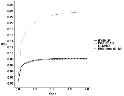
Figure 2: Average IBS for all methods in simulation case 1.

Table 3: Average c-index measures over 50 iterations in each simulation case.

	Case 1	Case 2	Case 3
BVSNLP	0.890	0.881	0.960
ISIS-SCAD	0.895	0.876	0.841
GLMNET	0.911	0.908	0.970

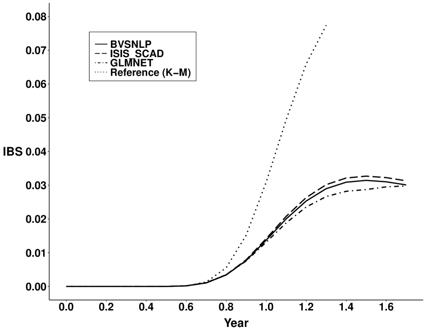
(a) Simulation case 2.

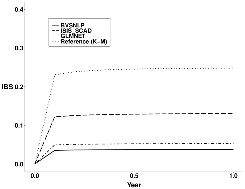
(b) Simulation case 3.

Figure 3: IBS plots for simulation cases 2 and 3.

5 Application to Real Data

We applied our method to selected genes associated with patient survival times for two common cancer types using datasets from The Cancer Genome Atlas (TCGA) projects: kidney renal clear cell carcinoma (KIRC) (Cancer Genome Atlas Research Network, 2013) and kidney renal papillary cell carcinoma (KIRP) (Cancer Genome Atlas Research Network, 2016). We compared the performance of our algorithm to ISIS-SCAD (Fan et al., 2010), GLMNET (Friedman et al., 2010) and Stability Selection (Meinshausen and Bühlmann, 2010). Stability Selection was combined with a high-dimensional selection algorithm, such as GLMNET, and selects the most stable features for a given level of Type I error. To run the Stability Selection method, we used the c060 R package (Sill et al., 2014) and the recommended values for function arguments.

We included patients’ “Age, Gender” and a clinical stage variable, “Stage”, in the design matrix. On the advice of a clinician, the “Stage” variable was developed by combining the histological stage, pathological stage and clinical stage into one variable that is a summary of how advanced each subject’s cancer was when the tissue sample was taken.“Stage”, like “Gender”, is a categorical variable but with three levels, where “Stage $i$” represents the $i^{th}$ class of that variable; “Stage 3” represents the most advanced stage. To remove stromal contaminations from the gene expression data, the DeMixT algorithm (Wang et al., 2017) was performed on the design matrix and the tumor-specific expression data were used in the analyses for all algorithms.

The predictive performance was measured by a time-dependent AUC, as discussed in Section 3.3, based on a five-fold cross-validation. The observations in each fold were randomly chosen under a constraint which balanced censoring rate between folds. The AUC values were computed for the test set using the model that was obtained by performing variable selection on the training set. The selected covariates for each cancer type were also compared. For our method, we report the covariates associated with the highest posterior probability model. The hyperparameter $\tau$ of the piMOM prior was selected using the algorithm in Section 3.1 with $\alpha=0.1$ as the mode of the piMOM prior. This is our choice of $\alpha$ for real datasets. The results for each cancer type are discussed in separate sections below. Note that GLMNET has a random output when the hyperparameter is selected by cross-validation. As a result, based on the recommendation of the inventors of that algorithm, we ran it 100 times for each fold and took the average of results as the outcome for that fold.

We treated categorical variables “Stage” and “Gender”, as well as the continuous variable “Age”, as fixed covariates in our model. However, available ISIS-SCAD and Stability Selection software packages are not able to fix preselected covariates to be included in all models. For this reason, dummy variables associated to “Stage” and “Gender” were manually added to the design matrix and were subject to the selection procedure for those methods.

5.1 Kidney Renal Clear Cell Carcinoma (KIRC)

After removing covariates with missing expressions and observations with missing survival times, the KIRC dataset (Cancer Genome Atlas Research Network, 2013) contains 490 observations with 13,267 covariates, . The censoring rate for this dataset is 66.94%. Table 4 shows the covariates selected by each method. As mentioned previously, GLMNET produces random outputs at each run, and therefore, for this table, only the output for one of the runs are indicated; other runs produced a similar number of selected covariates.

Table 4: Selected genes and covariates for KIRC across different variable selection algorithms

BVSNLP	Age	Gender	Stage
	SUDS3	AR
ISIS-SCAD	Stage 3	AR	Age
	HEBP1	ATP2C1	GADD45A
	MTERF2	ADGRL3	GPSM1
	SERPINI1	SP6	ZNF815P
	INAFM2
GLMNET	Stage	AR	Age
	HEBP1	SEC61A2	TRMT6
	PCBP4	FAHD2A	MCM8
	E2F5	SLC5A6	NARF
	RAB28	DONSON	GPSM1
	HACD1	MARS	FASN
	TRAIP	RPL17P50	SLC26A6
	GPR162	INAFM2	ACACA
Stability Selection	Stage 3	AR	Age
	INAFM2

In addition to the categorical covariate “Stage”, BVSNLP selects “AR” and “SUDS3” in the HPPM as the most significant covariates in the design matrix. The posterior inclusion probabilities for “AR” and “SUDS3” are $0.80$ and $0.08$, respectively. The “Age”, “Gender”, and “Stage” were fixed in all models and thus were selected with probability $1$. The MAP estimates for the coefficients of “Age, Gender Male, Stage 2, Stage 3, AR” and “SUDS3” were $0.33,-0.11,0.45,1.61,-0.60$ and $0.36$, respectively. These coefficients indicate that patients with the most advanced stages of cancer had the poorest survival rates, and that a patient with a tumor sample characterized as advanced has a hazard rate that was $\exp(1.61)\approx 5$ times higher than a patient with tumor sample characterized as localized, when all other covariates were the same. These coefficients also show that the hazard rate in females is 1.12 times that in males, and age has an unfavorable impact on the hazard rate, as expected. Moreover, the negative sign for the “AR” gene indicates it has a favorable impact on survival for KIRC. “AR”, the Androgen Receptor gene, functions as a steroid-hormone activated transcription factor. It has been well documented that “AR” promotes the progression of renal cell carcinoma (RCC) through hypoxia-inducible factors HIF-2$\alpha$ and vascular endothelial growth factor regulation (Fenner, 2016). The favorable impact of the “AR” gene was also studied by Hata et al. (2017) in bladder cancer. “SUDS3” is a regulatory protein that is part of the SIN3A corepressor complex component that potentially has a role in tumor suppressor pathways through regulation of apoptosis. There was previous evidence of the down-regulation of the SIN3A gene in tumorigenesis of lung cancer (Suzuki et al., 2008).

It is noteworthy that the algorithm selected the same highest posterior probability model for different values of the hyperparameter $\tau$ in the range $[0.01,0.9]$. This shows the robustness of the proposed variable selection algorithm to the choice of hyperparameter $\tau$ for a range of plausible values.

For this particular run of GLMNET, a much larger model was selected with 24 variables including two of the variables reported by BVSNLP. ISIS-SCAD selected 13 covariates, which included the four covariates that were selected by the Stability Selection method. “AR” and the last level of “Stage” are the common covariates among all methods.

The time dependent AUC plot for all four methods, obtained by performing a five-fold cross validation, is depicted in Figure 4. BVSNLP has slightly better predictive accuracy than GLMNET and Stability Selection. However, it achieves this accuracy with a much sparser model. We investigated the covariates that were selected by each of those algorithms in all five folds and found that BVSNLP, in addition to those fixed covariates, selects only 10 unique genes in total, where ‘AR’ is selected in three of the five folds.

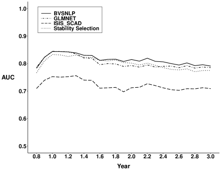
Figure 4: Average AUC of different variable selection methods based on a five fold cross-validation for KIRC dataset.

GLMNET selected 160 different covariates across all five folds. Only five out of 24 selected covariates in Table 4 were selected in all five training datasets in cross-validation. Those include “Age, Stage” and “AR”. GLMNET was run 100 times for each fold. ISIS-SCAD selected 45 different covariates, and only “Stage 3” was selected in all training datasets in cross-validation. The Stability Selection method selected sparser models compared to ISIS-SCAD and GLMNET by selecting 13 different covariates. It picked only “Age” and “Stage 3” in all five folds.

Figures 5(a) and 5(b) compare IBS and prediction error curves, respectively, between different methods for the KIRC dataset. These two measures were computed based on a five-fold cross-validation. Computation of IBS and prediction error were done using the R package pec (Mogensen et al., 2012). A benchmark model based on the Kaplan–Meier estimate, which includes no covariates, was also added to the figures as a reference for the comparison. The c-index measures are also reported in Table 5. The c-index was computed as it was in Section 4 using the dynpred package in R.

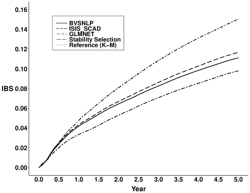
(a) IBS

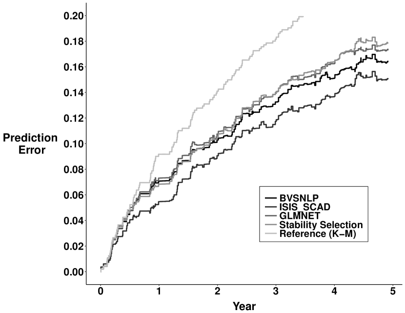
(b) Prediction Error

Figure 5: IBS and prediction error of BVSNLP for the KIRC dataset.

Table 5: Average c-index measure of different methods for the KIRC dataset.

	BVSNLP	GLMNET	ISIS-SCAD	Stability Selection
c-index measure	0.804	0.816	0.846	0.797

GLMNET has almost the same IBS curve as the reference Kaplan–Meier curve. BVSNLP outperforms ISIS-SCAD, and Stability selection has the best IBS performance among all. For prediction error curves, BVSNLP is second to ISIS-SCAD, and GLMNET and Stability Selection have almost the same performance. A different behavior can be seen for c-index measures where GLMNET and ISIS-SCAD have higher c-indices than BVSNLP.

BVSNLP was run on 120 CPUs, Stability Selection was run on four CPUs, while GLMNET and ISIS-SCAD were run on a single CPU. The average runtime for different methods in each fold of the cross validation was 6.4, 180, 5, and 1.3 minutes for BVSNLP, GLMNET, ISIS-SCAD and Stability Selection.

In our previous study of binary outcomes using the same dataset (Nikooienejad et al., 2016), we performed hierarchical clustering on the deconvolved tumor-specific expression matrix and identified two clusters of patient samples. We saw these two groups of patients present significantly different survival outcomes and, therefore, assigned good vs. bad survival to the groups. The dichotomization was based solely on the clustering results of deconvolved gene expression levels. Survival times and censoring did not play any role in that process. However, there was a loss of information in dichotomizing a survival dataset and analyzing it with logistic regression. Now, with BVSNLP, we are able to use the original survival time to event with censoring information. To compare the biological implications between the two analyses, we looked for known expression regulation networks between the gene sets found in the binary analysis, SAV1 and NUMBL, and the new genes found in this analysis, AR and SUDS3, using Pathway Studio^® (Nikitin et al., 2003; Elsevier, 2018). We found that the well-studied cancer genes TGFB1, BCL2, PPARG, NEDD4, and CTNNB1, and a regulatory microRNA, MIR21, constitute the shortest paths between SAV1 and AR. Similarly, we found cancer genes CDKN1A, WNT3A, two genes that determine cell fate (SOX17 (connected with CTNNB1) and NANOG) and PAX6 that regulates transcription, to constitute the shortest paths between NUMBL and SUDS3. These are depicted in Section 6 of the LABEL:suppA (Nikooienejad et al., 2020) . These findings suggest a high biological consistency between our two analyses that used BVSNLP to select features for binary and survival outcomes.

In summary, the binary model using SAV1 and NUMBL to predict overall survival of patients with kidney cancer is not as effective as the model using AR and SUDS3, as shown in Figure 6. Thus, although the findings of Nikooienejad et al. (2016) were biologically justified, some limitations were associated with those findings due to the information loss incurred by clustering and dichotomizing the data, and the BVSNLP survival model provides better insight on the genes associated with this cancer type.

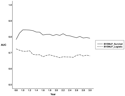
Figure 6: Comparison between BVSNLP model selection using survival and dichotomized versions of the KIRC dataset.

5.2 Kidney Renal Papillary Cell Carcinoma (KIRP)

The KIRP dataset (Cancer Genome Atlas Research Network, 2016) contains 244 samples with 13,335 covariates (after necessary data cleaning) and has a fairly high censoring rate of 85.7%. The covariates selected by each method are summarized in Table 6.

In addition to the fixed covariates “Age, Gender”, and “Stage”, BVSNLP selects the “CDK1” gene in the HPPM as the most significant covariate in the design matrix. The posterior inclusion probability for “CDK1” was $0.12$. The MAP estimates for the coefficients of “Age, Gender Male, Stage 2, Stage 3” and “CDK1” were $0.12,-0.10,0.11,0.79$ and $1.13$, respectively. This shows that a unit increase in “CDK1” (Cyclin dependent kinase 1) gene expression increases the hazard rate by a factor of three for given values of the other covariates. CDK1 is a cell cycle regulator and has been reported previously as a prognostic marker gene for various cancer types. Many experimental studies have been performed to further understand the molecular mechanism behind the complex functions of CDK1 (Malumbres and Barbacid, 2009). This is the first time, however, that CDK1 has been reported as a prognostic marker gene in human data for papillary renal cell carcinoma. As expected, patients at the most advanced stage cancer have a hazard rate that is 2.2 times higher than patients at a localized stage of cancer, given the values of all other covariates. As in the case of KIRC patients, age and male gender have unfavorable and favorable impacts on the hazard rate, respectively.

Table 6: Selected covariates for KIRP across different variable selection algorithms

BVSNLP	Age	Gender	Stage
	CDK1
ISIS-SCAD	CDK1	COL6A1	C19orf33
GLMNET	No covariates were selected
Stability Selection	Stage 3	MTC02P12	RPL39P3

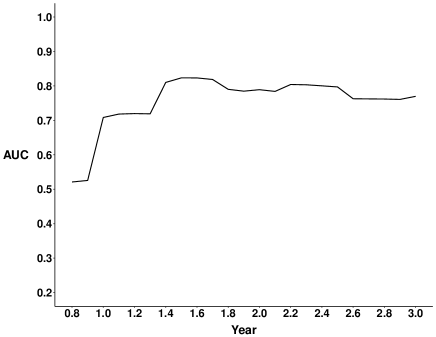
Figure 7: Average AUC of BVSNLP based on a five fold cross-validation for the KIRP dataset.

Surprisingly, GLMNET does not select any covariates. Stability Selection picked three covariates, with only “Stage 3” in common with BVSNLP. As in the previous dataset, we tested BVSNLP for different choices of $\tau$ in the interval $[0.01,0.9]$, and the same model was selected for all values within this range. The total runtime of BVSNLP for this dataset was around five minutes using 120 CPUs.

Figure 7 shows the predictive accuracy for the proposed method based on a five-fold cross-validation. The outcomes for GLMNET, ISIS-SCAD and Stability Selection are not displayed in the plot because those methods did not converge or failed to produce results for at least one of the five folds in the cross-validation experiment. The small AUC values in this plot for $t<1$ warrant comment. Because there were few events soon after entry of tissue samples into the TCGA database, the AUC for early timepoints falls close to the 50% benchmark reflecting no predictive value.

Figures 8(a) and 8(b), respectively, depict IBS and prediction error curves of the BVSNLP method, based on a five-fold cross validation for the KIRP dataset, and compares it to the reference curve obtained by the Kaplan–Meier method. The c-index measure for the BVSNLP method is 0.876. The average runtime for BVSNLP in each fold of the cross-validation was 3.6 minutes on 120 CPUs.

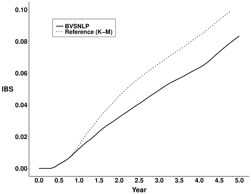
(a) IBS

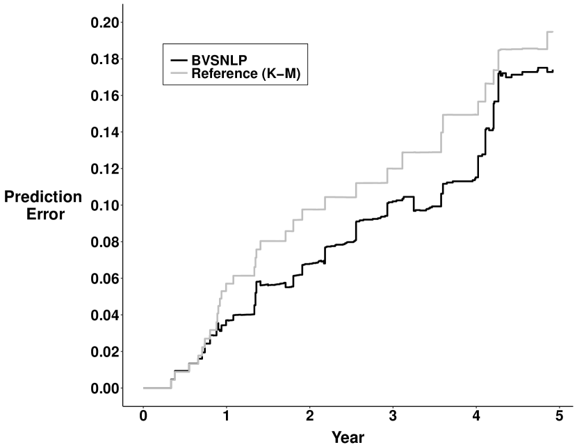
(b) Prediction Error

Figure 8: IBS and prediction error of BVSNLP for the KIRP dataset.

6 Discussion

In this article a Bayesian variable selection method, BVSNLP, was proposed for selecting variables in high and ultrahigh dimensional datasets with survival time as outcomes. BVSNLP uses an inverse moment nonlocal prior density on nonzero regression coefficients. Analyses of simulated and real data suggest that BVSNLP performs comparably or better than other existing methods for variable selection for survival data. Moreover, the real data results indicated that the proposed algorithm is robust to the choice of the hyperparameter $\tau$ in the piMOM prior for values of $\tau$ in the range $[0.01,0.9]$.

Various outputs are provided by the algorithm. These include the HPPM, MPM and the posterior inclusion probability for each covariate in the model. For real datasets, Bayesian model averaging is used to incorporate uncertainty in selected models when computing time dependent AUC plots using Uno’s method (Uno et al., 2007). Finally, an R package named BVSNLP has been implemented to make the algorithm freely available and adaptable to interested researchers. The package can be run in parallel fashion where hundreds of CPUs can be exploited in order to increase the number of visited models in the search for the highest posterior probability model. The BVSNLP package is available in the R repository, CRAN, at https://CRAN.R-project.org/package=BVSNLP. The user manual for the package is also available from this site.

Two real cancer genomic datasets from the TCGA website were considered in this article. Compared to other methods, BVSNLP found sparser models with biologically relevant genes. The proposed method showed a reliable predictive accuracy as measured by AUC using substantially fewer variables.

We have based our assessments on time dependent AUC and biological interpretation of the results, but other measures, like IBS, prediction error and the concordance index (also known as the c-index or Harrell’s c-index) were also reported. Difficulties associated with such measures are identified in Blanche et al. (2018). In particular, the authors of that article demonstrate that the concordance index can favor misspecified models over the correctly specified model because it is based on the order of event times rather than the event status at the prediction horizon. This may explain the slightly higher c-index values for GLMNET in both simulation and real datasets. The time dependent AUC does not suffer from this deficiency. Of course, different evaluation criteria can be expected to result in different rankings of models, and criteria that emphasize prediction error over low false positive rates can be expected to favor larger models. Similarly, criteria that place a higher premium on eliminating false positives will tend to select smaller models.

Acknowledgments: Portions of this research were conducted with the advanced computing resources provided by Texas A&M High Performance Research Computing (HPRC).

References

- Antoniadis et al. (2010) Antoniadis, A., Fryzlewicz, P., and Letué, F. (2010). The dantzig selector in cox’s proportional hazards model. Scandinavian Journal of Statistics, 37(4), 531–552.
- Barbieri and Berger (2004) Barbieri, M. M. and Berger, J. O. (2004). Optimal predictive model selection. The Annals of Statistics, 32(3), 870–897.
- Bender et al. (2005) Bender, R., Augustin, T., and Blettner, M. (2005). Generating survival times to simulate cox proportional hazards models. Statistics in Medicine, 24(11), 1713–1723.
- Berger et al. (1999) Berger, J. O., Liseo, B., Wolpert, R. L., et al. (1999). Integrated likelihood methods for eliminating nuisance parameters. Statistical Science, 14(1), 1–28.
- Blanche et al. (2018) Blanche, P., Kattan, M. W., and Gerds, T. A. (2018). The c-index is not proper for the evaluation of -year predicted risks. Biostatistics, 20(2), 347–357.
- Cancer Genome Atlas Research Network (2013) Cancer Genome Atlas Research Network (2013). Comprehensive molecular characterization of clear cell renal cell carcinoma. Nature, 499(7456), 43–49.
- Cancer Genome Atlas Research Network (2016) Cancer Genome Atlas Research Network (2016). Comprehensive molecular characterization of papillary renal-cell carcinoma. New England Journal of Medicine, 374(2), 135–145.
- Cox (1972) Cox, D. R. (1972). Regression models and life-tables. Journal of the Royal Statistical Society. Series B (Methodological), 36(2), 187–220.
- Cox and Oakes (1984) Cox, D. R. and Oakes, D. (1984). Analysis of Survival Data, volume 21. CRC Press.
- Elsevier (2018) Elsevier (2018). PathwayStudio®, volume pathwaystudio.com. Elsevier Inc.
- Fan and Li (2002) Fan, J. and Li, R. (2002). Variable selection for cox’s proportional hazards model and frailty model. Annals of Statistics, 30(1), 74–99.
- Fan and Lv (2008) Fan, J. and Lv, J. (2008). Sure independence screening for ultrahigh dimensional feature space. Journal of the Royal Statistical Society: Series B (Statistical Methodology), 70(5), 849–911.
- Fan et al. (2010) Fan, J., Feng, Y., Wu, Y., et al. (2010). High-dimensional variable selection for cox’s proportional hazards model. In Borrowing Strength: Theory Powering Applications–A Festschrift for Lawrence D. Brown, pages 70–86. Institute of Mathematical Statistics.
- Faraggi and Simon (1998) Faraggi, D. and Simon, R. (1998). Bayesian variable selection method for censored survival data. Biometrics, 54(4), 1475–1485.
- Fenner (2016) Fenner, A. (2016). Kidney cancer: Ar promotes rcc via lncrna interaction. Nature Reviews Urology, 13(5), 242.
- Friedman et al. (2010) Friedman, J., Hastie, T., and Tibshirani, R. (2010). Regularization paths for generalized linear models via coordinate descent. Journal of Statistical Software, 33(1), 1–22.
- George and McCulloch (1997) George, E. I. and McCulloch, R. E. (1997). Approaches for bayesian variable selection. Statistica Sinica, 7(2), 339–373.
- Gerds and Schumacher (2006) Gerds, T. A. and Schumacher, M. (2006). Consistent estimation of the expected brier score in general survival models with right-censored event times. Biometrical Journal, 48(6), 1029–1040.
- Ghosh (1988) Ghosh, J. (1988). Statistical information and likelihood: A collection of critical essays by dr. d. basu. Lect. Notes in Statist, 45.
- Harrell Jr et al. (1982) Harrell Jr, F. E., Califf, R. M., Pryor, D. B., Lee, K. L., Rosati, R. A., et al. (1982). Evaluating the yield of medical tests. JAMA, 247(18), 2543–2546.
- Hata et al. (2017) Hata, S., Ise, K., Azmahani, A., Konosu-Fukaya, S., McNamara, K. M., Fujishima, F., Shimada, K., Mitsuzuka, K., Arai, Y., Sasano, H., et al. (2017). Expression of ar, 5r1 and 5r2 in bladder urothelial carcinoma and relationship to clinicopathological factors. Life Sciences, 190, 15–20.
- Heagerty et al. (2000) Heagerty, P. J., Lumley, T., and Pepe, M. S. (2000). Time-dependent roc curves for censored survival data and a diagnostic marker. Biometrics, 56(2), 337–344.
- Held et al. (2016) Held, L., Gravestock, I., and Sabanés Bové, D. (2016). Objective bayesian model selection for cox regression. Statistics in Medicine, 35(29), 5376–5390.
- Ibrahim et al. (1999) Ibrahim, J. G., Chen, M.-H., and MacEachern, S. N. (1999). Bayesian variable selection for proportional hazards models. Canadian Journal of Statistics, 27(4), 701–717.
- Johnson (2005) Johnson, V. E. (2005). Bayes factors based on test statistics. Journal of the Royal Statistical Society: Series B (Statistical Methodology), 67(5), 689–701.
- Johnson and Rossell (2010) Johnson, V. E. and Rossell, D. (2010). On the use of non-local prior densities in bayesian hypothesis tests. Journal of the Royal Statistical Society: Series B (Statistical Methodology), 72(2), 143–170.
- Johnson and Rossell (2012) Johnson, V. E. and Rossell, D. (2012). Bayesian model selection in high-dimensional settings. Journal of the American Statistical Association, 107(498), 649–660.
- Kalbfleisch and Prentice (1980) Kalbfleisch, J. and Prentice, R. (1980). The statistical analysis of time failure data. John Wiley and Sons New York.
- Liu and Nocedal (1989) Liu, D. C. and Nocedal, J. (1989). On the limited memory bfgs method for large scale optimization. Mathematical Programming, 45(1-3), 503–528.
- Malumbres and Barbacid (2009) Malumbres, M. and Barbacid, M. (2009). Cell cycle, cdks and cancer: a changing paradigm. Nature Rseviews Cancer, 9(3), 153.
- Meinshausen and Bühlmann (2010) Meinshausen, N. and Bühlmann, P. (2010). Stability selection. Journal of the Royal Statistical Society: Series B (Statistical Methodology), 72(4), 417–473.
- Mogensen et al. (2012) Mogensen, U. B., Ishwaran, H., and Gerds, T. A. (2012). Evaluating random forests for survival analysis using prediction error curves. Journal of Statistical Software, 50(11), 1–23.
- Morris et al. (2019) Morris, T. P., White, I. R., and Crowther, M. J. (2019). Using simulation studies to evaluate statistical methods. Statistics in Medicine, 38(11), 2074–2102.
- Nikitin et al. (2003) Nikitin, A., Egorov, S., Daraselia, N., and Mazo, I. (2003). Pathway studio–the analysis and navigation of molecular networks. Bioinformatics, 19(16), 2155–2157.
- Nikooienejad et al. (2020) Nikooienejad, A. et al. (2020). Supplement to “bayesian variable selection for survival data using inverse moment priors”.
- Nikooienejad et al. (2016) Nikooienejad, A., Wang, W., and Johnson, V. E. (2016). Bayesian variable selection for binary outcomes in high-dimensional genomic studies using non-local priors. Bioinformatics, 32(9), 1338–1345.
- Scott et al. (2010) Scott, J. G., Berger, J. O., et al. (2010). Bayes and empirical-bayes multiplicity adjustment in the variable-selection problem. The Annals of Statistics, 38(5), 2587–2619.
- Sha et al. (2006) Sha, N., Tadesse, M. G., and Vannucci, M. (2006). Bayesian variable selection for the analysis of microarray data with censored outcomes. Bioinformatics, 22(18), 2262–2268.
- Shin et al. (2018) Shin, M., Bhattacharya, A., and Johnson, V. E. (2018). Scalable bayesian variable selection using nonlocal prior densities in ultrahigh-dimensional settings. Statistica Sinica, 28(2), 1053–1078.
- Sill et al. (2014) Sill, M., Hielscher, T., Becker, N., and Zucknick, M. (2014). c060: Extended inference with lasso and elastic-net regularized cox and generalized linear models. Journal of Statistical Software, 62(5), 1–22.
- Suzuki et al. (2008) Suzuki, H., Ouchida, M., Yamamoto, H., Yano, M., Toyooka, S., Aoe, M., Shimizu, N., Date, H., and Shimizu, K. (2008). Decreased expression of the sin3a gene, a candidate tumor suppressor located at the prevalent allelic loss region 15q23 in non-small cell lung cancer. Lung Cancer, 59(1), 24–31.
- Tibshirani et al. (1997) Tibshirani, R. et al. (1997). The lasso method for variable selection in the cox model. Statistics in Medicine, 16(4), 385–395.
- Uno et al. (2007) Uno, H., Cai, T., Tian, L., and Wei, L. (2007). Evaluating prediction rules for t-year survivors with censored regression models. Journal of the American Statistical Association, 102(478), 527–537.
- van Houwelingen and Putter (2011) van Houwelingen, H. and Putter, H. (2011). Dynamic Prediction in Clinical Survival Analysis. CRC Press.
- Wang et al. (2017) Wang, Z., Morris, J. S., Cao, S., Ahn, J., Liu, R., Tyekucheva, S., Li, B., Lu, W., Tang, X., Wistuba, I. I., et al. (2017). Transcriptome deconvolution of heterogeneous tumor samples with immune infiltration. bioRxiv, page 146795.
- Zhang and Lu (2007) Zhang, H. H. and Lu, W. (2007). Adaptive lasso for cox’s proportional hazards model. Biometrika, 94(3), 691–703.