Shape from Shading through Shape Evolution

Abstract

In this paper, we address the shape-from-shading problem by training deep networks with synthetic images. Unlike conventional approaches that combine deep learning and synthetic imagery, we propose an approach that does not need any external shape dataset to render synthetic images. Our approach consists of two synergistic processes: the evolution of complex shapes from simple primitives, and the training of a deep network for shape-from-shading. The evolution generates better shapes guided by the network training, while the training improves by using the evolved shapes. We show that our approach achieves state-of-the-art performance on a shape-from-shading benchmark.

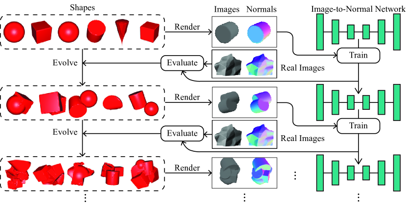
Figure 1: The overview of our approach. Starting from simple primitives such as spheres and cubes, we evolve a population of complex shapes. We render synthetic images from the shapes to incrementally train a shape-from-shading network. The performance of the network on a validation set of real images is then used to guide the shape evolution.

1 Introduction

Shape from Shading (SFS) is a classic computer vision problem at the core of single-image 3D reconstruction  [44]. Shading cues play an important role in recovering geometry and are especially critical for textureless surfaces.

Traditionally, Shape from Shading has been approached as an optimization problem where the task is to solve for a plausible shape that can generate the pixels under a Lambertian shading model [43, 15, 5, 4, 3]. The key challenge is to design an appropriate optimization objective to sufficiently constrain the solution space, and to design an optimization algorithm to find a good solution efficiently.

In this paper, we address Shape from Shading by training deep networks on synthetic images. This follows an emerging line of work on single-image 3D reconstruction that combines synthetic imagery and deep learning [36, 25, 24, 45, 29, 37, 10, 42, 6]. Such an approach does away with the manual design of optimization objectives and algorithms, and instead trains a deep network to directly estimate shape. This approach can take advantage of a large amount of training data, and has shown great promise on tasks such as view point estimation [36], 3D object reconstruction and recognition [37, 10, 42], and normal estimation in indoor scenes [45].

One limitation of this data-driven approach, however, is availability of 3D shapes needed for rendering synthetic images. Existing approaches have relied on manually constructed [8, 41, 1] or scanned shapes [9]. But such datasets can be expensive to build. Furthermore, while synthetic datasets can be augmented with varying viewpoints and lighting, they are still constrained by the number of distinct shapes, which may limit the ability of trained models to generalize to real images.

An intriguing question is whether it would be possible to do away with manually curated 3D shapes while still being able to use synthetic images to train deep networks. Our key hypothesis is that shapes are compositional and we should be able to compose complex shapes from simple primitives. The challenge is how to enable automatic composition and how to ensure that the composed shapes are useful for training deep networks.

We propose an evolutionary algorithm that jointly generates 3D shapes and trains a shape-from-shading deep network. We evolve complex shapes entirely from simple primitives such as spheres and cubes, and do so in tandem with the training of a deep network to perform shape from shading. The evolution of shapes and the training of a deep network collaborate—the former generates shapes needed by the latter, and the latter provides feedback to guide the former. Our approach is significantly novel compared to prior works that use synthetic images to train deep networks, because they have all relied on manually curated shape datasets [36, 24, 45, 37].

In this algorithm, we represent each shape using an implicit function [28]. Each function is composed of simple primitives, and the composition is encoded as a computation graph. Starting from simple primitives such as spheres and cubes, we evolve a population of shapes through transformations and compositions defined over graphs. We render synthetic images from each shape in the population and use the synthetic images to train a shape-from-shading network. The performance of the network on a validation set of real images is then used to define the fitness score of each shape. In each round of the evolution, fitter shapes have better chance of survival whereas less fit shapes tend to be eliminated. The end result is a population of surviving shapes, along with a shape-from-shading network trained with them. Fig. 1 illustrates the overall pipeline.

The shape-from-shading network is incrementally trained in a way that is tightly integrated with shape evolution. In each round of evolution, the network is fine-tuned separately with each shape in the population, spawning one new network instance per shape. Then the best network instance advances to the next round while the rest are discarded. In other words, the network tries updating its weights using each newly evolved shape, and the best weights are kept to the next round.

We evaluate our approach using the MIT-Berkeley Intrinsic Images dataset [5]. Experiments demonstrate that we can train a deep network to achieve state-of-the-art performance on real images using synthetic images rendered entirely from evolved shapes, without the help of any manually constructed or scanned shapes. In addition, we present ablation studies which support the design of our evolutionary algorithm.

Our results are significant in that we demonstrate that it is potentially possible to completely automate the generation of synthetic images used to train deep networks. We also show that the generation procedure can be effectively adapted, through evolution, to the training of a deep network. This opens up the possibility of training 3D reconstruction networks with a large number of shapes beyond the reach of manually curated shape collections.

To summarize, our contributions are twofold: (1) we propose an evolutionary algorithm to jointly evolve 3D shapes and train deep networks, which, to the best of our knowledge, is the first time this has been done; (2) we demonstrate that a network trained this way can achieve state-of-the-art performance on a real-world shape-from-shading benchmark, without using any external dataset of 3D shapes.

2 Related Work

Recovering 3D properties from a single image is one of the most fundamental problems of computer vision. Early works mostly focused on developing analytical solutions and optimization techniques, with zero or minimal learning [13, 44, 5, 4, 3]. Recent successes in this direction include the SIRFS algorithm by Barron and Malik [5], the local shape from shading method by Xiong et al. [43], and “polynomial SFS” algorithm by Ecker and Jepson [15]. All these methods have interpretable, “glass box” models with elegant insights, but in order to maintain analytical tractability, they have to make substantial assumptions that may not hold in unconstrained settings. For example, SIRFS [5] assumes a known object boundary, which is often unavailable in practice. The method by Xiong et al. assumes quadratically parameterized surfaces, which has difficulties approximating sharp edges or depth discontinuities.

Learning-based methods are less interpretable but more flexible. Seminal works include an MRF-based method proposed by Hoiem et al. [19] and the Make3D [32] system by Saxena et al. Cole et al. [12] proposed a data-driven method for 3D shape interpretation by retrieving similar image patches from a training set and stitching the local shapes together. Richter and Roth [30] used a discriminative learning approach to recover shape from shading in unknown illumination. Some recent works have used deep neural networks for predicting surface normals [40, 2] or depth [16, 39, 7] and have shown state-of-the-art results.

Learning-based methods cannot succeed without high-quality training data. Recent years have seen many efforts to acquire 3D ground truth from the real world, including ScanNet [14], NYU Depth [26], the KITTI Vision Benchmark Suite [17], SUN RGB-D [33], B3DO [22], and Make3D [32], all of which offer RGB-D images captured by depth sensors. The MIT-Berkeley Intrinsic Images dataset [5] provides real world images with ground truth on shading, reflectance, normals in addition to depth.

In addition to real world data, synthetic imagery has also been explored as a source of supervision. Promising results have been demonstrated on diverse 3D tasks such as pose estimation [36, 24, 1], optical flow [6], object reconstruction [37, 10], and surface normal estimation [45]. Such advances have been made possible by concomitant efforts to collect 3D content needed for rendering. In particular, the 3D shapes have come from a variety of sources, including online CAD model repositories [8, 41], interior design sites [45], video games [29, 31], and movies [6].

The collection of 3D shapes, from either the real world or a virtual world, involves substantial manual effort—the former requires depth sensors to be carried around whereas the latter requires human artists to compose the 3D models. Our work explores a new direction that automatically generates 3D shapes to serve an end task, bypassing real world acquisition or human creation.

Our work draws inspiration from the work of Clune & Lipson [11], which evolves 3D shapes as Compositional Pattern Producing Networks [34]. Our work differs from theirs in two important aspects. First, Clune & Lipson perform only shape generation, particularly the generation of interesting shapes, where interestingness is defined by humans in the loop. In contrast, we jointly generate shapes and train deep networks, which, to the best of our knowledge, is the first this has been done. Second, we use a significantly different evolution procedure. Clune & Lipson adopt the NEAT algorithm [35], which uses generic graph operations such as insertion and crossover at random nodes, whereas our evolution operations represent common shape “edits” such as translation, rotation, intersection, and union, which are chosen to optimize the efficiency of evolving 3D shapes.

3 Shape Evolution

Our shape evolution follows the setup of a standard genetic algorithm [20]. We start with an initial population of shapes. Each shape in the population receives a fitness score from an external evaluator. Then the shapes are sampled according to their fitness scores, and undergo random geometric operations to form a new population. This process then repeats for successive iterations.

3.1 Shape Representation

We represent shapes using implicit surfaces [28]. An implicit surface is defined by a function $F:\mathbb{R}^{3}\rightarrow\mathbb{R}.$ that maps a 3D point to a scalar. The surface consists of points $(x,y,z)$ that satisfy the equation:

$$F(x,y,z)=0.$$

And if we define the points $F(x,y,z)<0$ as the interior, then a solid shape is constructed from this function $F$. Note that the shape is not guaranteed to be closed, i.e., may have points at infinity. A simple workaround is to always confine the points within a cube [11].

Our initial shape population consists of four common shapes— sphere, cylinder, cube, and cone, which can be represented by the functions below:

$$\begin{array}[]{ll}\text{Sphere}:&F(x,y,z)=x^{2}+y^{2}+z^{2}-R^{2}\\ \text{Cylinder}:&F(x,y,z)=\max\left(\frac{x^{2}+y^{2}}{R^{2}},\frac{|z|}{H}\right)-1\\ \text{Cube}:&F(x,y,z)=\max(|x|,|y|,|z|)-\frac{L}{2}\\ \text{Cone}:&F(x,y,z)=\max(\frac{x^{2}+y^{2}}{R^{2}}-\frac{z^{2}}{H^{2}},-z,z-H)\end{array}$$ (1)

An advantage of implicit surfaces is that the composition of shapes can be easily expressed as the composition of functions, and a composite function can be represented by a (directed acyclic) computation graph, in the same way a neural network is represented as a computation graph.

Suppose a computation graph $G=(V,E)$. It includes a set of nodes $V=\{x,y,z\}\cup\{v_{1},v_{2},\cdots\}\cup\{t\}$, which includes three input nodes $\{x,y,z\}$, a variable number of internal nodes $\{v_{1},v_{2},\cdots\}$, and a single output node $t$. Each node $v\in V$ (excluding input nodes) is associated with a scalar bias $b_{v}$, a reduction function $r_{v}$ that maps a variable number of real values to a single scalar, and an activation function $\phi_{v}$ that maps a real value to a new value. In addition, each edge $e\in E$ is associated with a weight $w_{e}$.

It is worth noting that different from a standard neural network or a Compositional Pattern Producing Network (CPPN) that only uses sum as the reduction function, our reduction function can be sum, max or min. As will become clear, this is to allow straightforward composition of shapes.

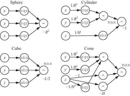
Figure 2: The computation graphs of four primitive shapes defined in Eq. 1. The unlabeled edge weight and node bias are $0$, and the unlabeled reduction function is sum.

To evaluate the computation graph, each node takes the weighted activations of its predecessors and applies the reduction function, followed by the activation function plus the bias. Fig. 2 illustrates the graphs of the functions defined in Eq. 1.

Shape Transformation

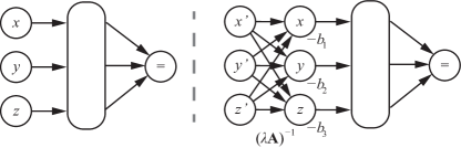
Figure 3: Shape transformation represented by graph operation. Left: the graph of the shape before transformation. Right: the graph of the shape after transformation.

To evolve shapes, we define graph operations to generate new shapes from existing ones. We first show how to transform an individual shape. Given an existing shape represented by $F(x,y,z)$, let $F(T(x,y,z))$ represent a transformed shape, where $T:\mathbb{R}^{3}\rightarrow\mathbb{R}^{3}$ is a 3D-to-3D map. It is easy to verify that $F(T(x,y,z))$ represents the transformed shape under translation, rotation, and scaling if we define $T$ as

$$T(x,y,z)=(\lambda\mathbf{A})^{-1}[x,y,z]^{\mathsf{T}}-\mathbf{b}\text{,}$$

where $\mathbf{A}$ is a rotation matrix, $\lambda$ is the scalar, and the $\mathbf{b}$ is the translation vector. Note that for simplicity our definitions have only included a single global scalar, but more flexibility can be easily introduced by allowing different scalars along different axes or an arbitrary invertible matrix $\mathbf{A}$.

This shape transformation can also be expressed in terms of a graph transformation, as illustrated in Fig. 3. Given the original graph of the shape, we insert 3 new input nodes $x^{\prime},y^{\prime},z^{\prime}$ before the original input nodes, connect new nodes to the original nodes with weights corresponding to the elements of the matrix $(\lambda\mathbf{A})^{-1}$, and set the biases of the original nodes to the vector $-\mathbf{b}$.

Shape Composition

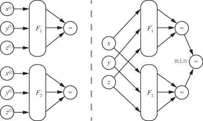
Figure 4: The union of two shapes represented by graph merging. Left: the respective graphs of the two shapes to be unioned. Right: the graph of the unioned shape.

In addition to transforming individual shapes, we also define binary operations over two shapes. This allows complex shapes to emerge from the composition of simple ones. Suppose we have two shapes with the implicit representations $F_{1}(x,y,z)$ and $F_{2}(x,y,z)$. As a basic fact [28], the union, intersection, and difference of the two can be represented as follows:

$$\begin{split}F_{\mathrm{union}}(x,y,z)&=\min(F_{1}(x,y,z),F_{2}(x,y,z))\\ F_{\mathrm{intersection}}(x,y,z)&=\max(F_{1}(x,y,z),F_{2}(x,y,z))\\ F_{\mathrm{difference(1,2)}}(x,y,z)&=\max(F_{1}(x,y,z),-F_{2}(x,y,z))\text{.}\end{split}$$

In terms of graph operations, composing two shapes together corresponds to merging two graphs. As illustrated by Fig. 4, we merge the input nodes of the two graphs and add a new output node that is connected to the two original output nodes. We set the reduction function (max, min, or sum) and the weights of the incoming edges to the new output node according to the specific composition chosen.

3.2 Evolution Algorithm

Our evolution process follows a standard setup. It starts with an initial population of $n$ shapes: $\{s_{1},s_{2},\cdots,s_{n}\}$, all of which are primitive shapes described in Eq. 1. Next, $m$ new shapes ($\{s^{\prime}_{1},s^{\prime}_{2},\cdots,s^{\prime}_{m}\}$) are created from two randomly sampled existing shapes (i.e., two parent shapes). Specifically, the two parent shapes each undergo a random rotation, a random scaling and a random translation, and are then combined by a random set operation chosen from union, intersection and difference to generate a new child shape. Now, the population consists of a total of $n+m$ ($n$ parent shapes and $m$ child shapes). Each shape is then evaluated and given a fitness score, based on which $n$ shapes are selected to form the next population. This process is then repeated to evolve more complex shapes.

Having outlined the overall algorithm, we now discuss several specific designs we introduce to make our evolution more efficient and effective.

Fitness propagation

Simply evaluating fitness as a function of individual shape is suboptimal in our case. Our shapes are evolved based on composition, and to generate a new shape requires combining existing shapes. If we define fitness strictly on an individual basis, simple shape primitives, which may be useful in producing more complex shapes, can be eliminated during the early rounds of evolution. For example, suppose our goal is to evolve an implicit representation of a target shape. As the population nears the target shape, smaller and simpler cuts and additions are needed to further refine the population. However, if small, simple shapes, which poorly represent the target shape, have been eliminated, such refinement cannot take place.

We introduce fitness propagation to combat this problem. We propagate fitness scores from a child shape to its parents to account for the fact that a parent shape may not have a high fitness in itself, but nonetheless should remain in the population because it can be combined with others to yield good shapes. Suppose in one round of evolution, we evaluate each of the $n$ existing shapes and $m$ newly composed shapes and obtain $n+m$ fitness scores $\{f_{1},\cdots,f_{n},f^{\prime}_{1},\cdots,f^{\prime}_{m}\}$. But instead of directly assigning the scores, we propagate the $m$ fitness scores of the child shapes back to the parent shapes. A parent shape $f_{i}$ is assigned the best fitness score obtained by its children and itself:

$$f_{i}\leftarrow\max\left(\{f^{\prime}_{j}:s_{i}\in\pi(s^{\prime}_{j})\}\cup\{f_{i}\}\right),$$

where $\pi(s^{\prime}_{j})$ is the parents of shape $s^{\prime}_{j}$.

Computational resource constraint

Because shapes evolve through composition, in the course of evolution the shapes will naturally become more complex and have larger computation graphs. It is easy to verify that the size of the computational graph of a composed shape will at least double in the subsequent population. Thus without any constraint, the average computational cost of a shape will grow exponentially in the number of iterations as the population evolves, quickly depleting available computing resources before useful shapes emerge. To overcome this issue, we impose a resource constraint by capping the growth of the graphs to be linear in the number of rounds of evolution. If the number of nodes of a computation graph exceeds $\beta t$, where $\beta$ is a hyperparameter and $t$ is time, the graph will be removed from the population and will not be used to construct the next generation of shapes.

Discarding trivial compositions

A random composition of two shapes can often result in trivial combinations. For instance, the intersection of shape $A$ and shape $B$ may be empty, and the union of two shapes can be the same as one of the parent. We detect and eliminate such cases to prevent them from slowing down the evolution.

Promoting Diversity

Diversity of the population is important because it prevents the evolution process from overcommitting to a narrow range of directions. If the externally given fitness score is the only criterion for selection, shapes deemed less fit at the moment tend to go extinct quickly, and evolution can get stuck due to a homogenized population. Therefore, we incorporate a diversity constraint into our algorithm: a fixed proportion of the shapes in the population are sampled not based on fitness, but based on the size of their computation graph, with bigger shapes sampled proportionally less often.

4 Joint Training of Deep Network

The shapes are evolved in conjunction with training a deep network to perform shape-from-shading. The network takes a rendered image as input, and predicts the surface normal at each pixel. To train this network, we render synthetic images and obtain the ground truth normals using the evolved shapes.

The network is trained incrementally with a training set that consists of evolved shapes. Let $D_{i}$ be the training set after the $i$th iteration of the evolution, and let $N_{i}$ be the network at the same time. The training set is initialized to empty before the evolution starts, i.e. $D_{0}=\emptyset$, and the network is initialized with random weights.

In the $i$th evolution iteration, to compute the fitness score of a shape $d$ in the population, we fine-tune the current network $N_{i-1}$ with $D_{i-1}\cup\{d\}$—the current training set plus the shape in consideration—to produce a fine-tuned network $N^{d}_{i-1}$, which is evaluated on a validation set of real images to produce an error metric that is then used to define the fitness score of shape $d$. After we have evaluate the fitness of every shape in the population, we update the training set with the fittest shape $d^{*}_{i}$,

$$D_{i}=D_{i-1}\cup\{d^{*}_{i}\},$$

and set the $N^{d^{*}}_{i-1}$ as the current network,

$$N_{i}=N^{d^{*}}_{i-1}.$$

In other words, we maintain a growing training set for the network. In each evolution iteration, for each shape in the population we evaluate what would happen if add the shape to the training set and continue to train the network with the new training set. This is done for each shape in the population separately, resulting in as many new network instances as there are shapes in the current population. The best shape is then officially added to the training set, and the corresponding fine-tuned network is also kept while the other network instances are discarded.

5 Experiments

5.1 Standalone Evolution

We first experiment with shape evolution as a standalone module and study the role of several design choices. Similar to  [11], we evaluate whether our evolution process is capable of generating shapes close to a given target shape. We define the fitness score of an evolved shape as its intersection over union (IoU) of volume with the target shape.

Implementation details

To select the shapes during evolution, half of the population are sampled based on the rank $r$ of their fitness score (from high to low), with the selection probability set to $0.2^{r}$. The other half of the population are sampled based on the rank $s$ of their computation graph size (from small to large), with the relative selection probability set to $0.2^{s}$, in order to maintain diversity. To compute the volume, we voxelize the shapes to $32\times 32\times 32$ grids. The population size $n$ is $1000$ and the number of child shapes $m=1000$.

Results

We use two target shapes, a heart and a torus. Fig. 5 shows the two target shapes along with the fittest shape in the population as the evolution progresses. We can see that the evolution is able to produce shapes very close to the targets. Quantitatively, after around 600 iterations, the best IoU of the evolved shapes reaches $94.9\%$ for the heart and $93.5\%$ for the torus.

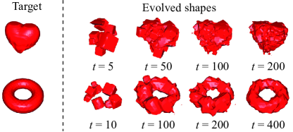
Figure 5: Evolution towards a target shape. Left: targets. Right: The fittest shapes in the population as the evolution progresses at different iterations.

We also study the effect of the design choices described in Sec. 3.2, including fitness propagation, discarding trivial compositions, and promoting diversity. Fig. 6 plots, for different combinations of these choices, the best IoU with the target shape (heart) versus evolution time, in terms of both wall time and the number of iterations. We can see that each of them is beneficial and enabling all three achieves fastest evolution in terms of wall time. Note that, the diversity constraint slows down evolution initially in terms of the number of iterations, but it prevents early saturation and is faster in terms of wall time because of lower computational cost in each iteration.

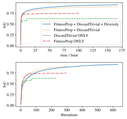
Figure 6: The best IoU with the target shape (heart) versus evolution time (top) and the number of iterations (bottom) for different combinations of design choices.

5.2 Joint Evolution and Training

We now evaluate our full algorithm that jointly evolves shapes and trains a deep network. We first describe in detail the setup of our individual components.

Setup of network training

We use a stacked hourglass network [27] as our shape-from-shading network. The network consists of a stack of 4 hourglasses, with 16 feature channels for each hourglass and 32 feature channels for the initial layers before the hourglasses. In each round of evolution, we fine-tune the network for $\tau=100$ iterations using RMSprop [38], a batch size of 4, and the mean angle error as the loss function. Before fine-tuning on the new dataset, we re-initialize the RMSprop optimizer.

Rendering synthetic images

To render shapes into synthetic images, we use the Mitsuba renderer [21], a physically based photorealistic renderer. We run the marching cubes algorithm [23] on the implicit function of a shape with a resolution of $64\times 64\times 64$ to generate the triangle mesh for rendering. We use a randomly placed orthographic camera, and a directional light with a random direction within $60^{\circ}$ of the viewing direction to ensure a sufficiently lit shape. All shapes are rendered with diffuse textureless surfaces, along with self occlusion and shadows. In addition to the images, we also generate ground truth surface normals.

Real images with ground truth

For both training and testing, we need a set of real-world images with ground truth of surface normals. For training, we need a validation set of real images to evaluate the fitness of shapes, which is defined as how well they help the performance of a shape-from-shading network on real images. For testing, we need a test set of real images to evaluate the performance of the final network.

We use the MIT-Berkeley Intrinsic Image dataset [5, 18] as the source of real images. It includes images of 20 objects captured in a lab setting; each object has two images, one with texture and the other textureless. We use the textureless version of the dataset because our method only evolves shape but not texture. We adopt the official 50-50 train-test split, using the 10 training images as the validation set for fitness evaluation and the 10 test images to evaluate the performance of the final network.

Setup of shape evolution

In each iteration of shape evolution, the population size is maintained at $n=100$, and $m=100$ new shapes are composed. To select the shapes, 90% of the population are sampled by a roulette wheel where the probability of each shape being chosen is proportional to its fitness score. The fitness score is the reciprocal of the mean angle error on the validation set. The remaining 10% are sampled using the diversity promoting strategy, where the shapes are sampled also based on the rank $s$ of their computation graph size (from small to large), with the relative selection probability set to $0.5^{s}$.

Evaluation Protocol

To evaluate the shape-from-shading performance of the final network, we use standard metrics proposed by prior work [40, 5]. We measure N-MAE and N-MSE, i.e. the mean angle distance (in radians) between the predicted normals and ground-truth normals, and the mean squared errors of the normal vectors. We also measure the fraction of the pixels whose normals are within 11.25, 22.5, 30 degrees angle distance of the ground-truth normals.

Since our network only accepts 128$\times$128 input size but the images in the MIT-Berkeley dataset have different sizes, we pad the images and scale them to 128$\times$128 to feed into the network, and then scale them back and crop to the original sizes for evaluation.

5.2.1 Baselines approaches

We compare with a number of baseline approaches including ablated versions of our algorithm. We describe them in detail below.

SIRFS

SIRFS [5] is an algorithm with state-of-the-art performance on shape from shading. It is primarily based on optimization and manually designed priors, with a small number of learned parameters. Our method only evolves shapes but not texture, so we compare with SIRFS using the textureless images. Because the published results [5] only textured objects from the MIT-Berkeley Intrinsic Image dataset, we obtained the results on textureless objects using their open source code.

Training with ShapeNet

We also compare a baseline approach that trains the shape-from-shading network using synthetic images rendered from an external shape dataset. We use a version of ShapeNet [8], a large dataset of 3D CAD models that consists of approximately 51,300 shapes. We evaluate two variants of this approach.

• ShapeNet-vanilla We train a single deep network on the synthetic images rendered using shapes in ShapeNet. Both the network structure and the rendering setting are the same as in the evolutionary algorithm. For every $\tau$ RMSprop iterations (the number of iterations used to fine-tune a network in the evolution algorithm), we record the validation performance and save the snapshot of the network. When testing, the snapshot with the best validation performance is used.

• ShapeNet-incremental Same as the first ShapeNet-incremental, except that we restart the RMSprop training every $\tau$ iterations, initializing from the latest weights. This is because in our evolution algorithm only the network weights are reloaded for incremental training, while the RMSprop training starts from scratch. We include this baseline to eliminate any advantage the restarts might bring in our evolution algorithm.

Ablated versions of our algorithm

We consider three ablated versions of our algorithm:

• Ours-no-feedback The fitness score is replaced by a random value, while all other parts of the algorithm remain unchanged. The shapes are still being evolved, and the networks are still being trained, but there is no feedback on how good the shapes are.

• Ours-no-evolution The evolution is disabled, which means the population remains to be the initial set of primitive shapes throughout the whole process. This ablated version is equivalent to training a set of networks on a fixed dataset and picking the one from $n+m$ networks that has the best performance on the validation set every $\tau$ training iterations.

• Ours-no-evolution-plus-ShapeNet The evolution is disabled, and maintain a population of $n+m$ network instances being trained simultaneously. For each $\tau$ iterations, the network with the best validation performance is selected and copied to replace the entire population. It is equivalent to Ours-no-evolution except that the primitive shapes are replaced by shapes randomly sampled from ShapeNet each time we render an image. This ablation is to evaluate whether our evolved shapes are better than ShapeNet shapes, controlling for any advantage our training algorithm might have even without any evolution taking place.

	Summary Stats $\uparrow$			Errors $\downarrow$
	$\leq 11.25^{\circ}$	$\leq 22.5^{\circ}$	$\leq 30^{\circ}$	MAE	MSE
Random∗	1.9%	7.5%	13.1%	1.1627	1.3071
SIRFS [5]	20.4%	53.3%	70.9%	0.4575	0.2964
ShapeNet-vanilla	12.7%	42.4%	62.8%	0.4831	0.2901
ShapeNet-incremental	15.2%	48.4%	66.4%	0.4597	0.2717
Ours-no-evolution-plus-ShapeNet	14.2%	53.0%	72.1%	0.4232	0.2233
Ours-no-evolution	17.3%	50.2%	66.1%	0.4673	0.2903
Ours-no-feedback	19.1%	49.5%	66.3%	0.4477	0.2624
Ours	21.6%	55.5%	73.5%	0.4064	0.2204

Table 1: The results of baselines and our approach on the test images. ^∗Measured by uniformly randomly outputting unit vectors on the $+z$ hemisphere.

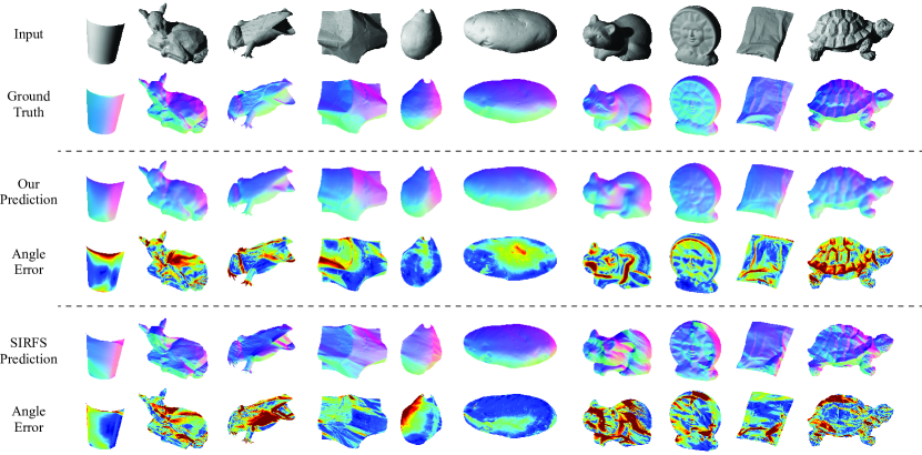
Figure 7: The qualitative results of our method and SIRFS [5] on the test data.

5.2.2 Results and analysis

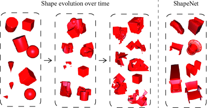
Figure 8: Example shapes at different stages of the evolution and shapes from ShapeNet.

Tab. 1 compares the baselines with our approach. We first see that the deep network trained through shape evolution outperforms the state-of-the-art SIRFS algorithm, without using any external dataset except for the 10 training images in the MIT-Berkeley dataset that are also used by SIRFS.

We also see that our algorithm outperforms all baselines trained on ShapeNet as well as all ablated versions. This shows that our approach can do away with an external shape dataset and generate useful shapes from simple primitives, and the evolved shapes are as useful as shapes from ShapeNet for this shape-from-shading task. Fig. 8 shows example shapes at different stages of the evolution, as well as shapes from ShapeNet, and Fig. 7 shows qualitative results of our method and SIRFS on the test data.

More specifically, the Ours-no-evolution-plus-ShapeNet ablation shows that our evolved shapes are actually more useful than ShapeNet for the task, although this is not surprising given that the evolution is biased toward being useful. Also it shows that the advantage our method has over using ShapeNet is due to evolution, not idiosyncrasies of our training procedure.

The Ours-no-evolution ablation shows that our good performance is not a result of well chosen primitive shapes, and evolution actually generates better shapes. The Ours-no-feedback ablation shows that the joint evolution and training is also important—random evolution can produce complex shapes, but without guidance from network training, the shapes are only slightly more useful than the primitives.

6 Conclusion

We have introduced a new algorithm to jointly evolve 3D shapes and train a shape-from-shading network through synthetic images. We show that our approach can achieve state-of-the-art performance on real images without using an external shape dataset.

Acknowledgments This work is partially supported by the National Science Foundation under Grant No. 1617767.

References

- [1] M. Aubry, D. Maturana, A. Efros, B. Russell, and J. Sivic. Seeing 3d chairs: exemplar part-based 2d-3d alignment using a large dataset of cad models. In CVPR, 2014.
- [2] A. Bansal, B. Russell, and A. Gupta. Marr Revisited: 2D-3D model alignment via surface normal prediction. In CVPR, 2016.
- [3] J. T. Barron and J. Malik. High-frequency shape and albedo from shading using natural image statistics. In Computer Vision and Pattern Recognition (CVPR), 2011 IEEE Conference on, pages 2521–2528. IEEE, 2011.
- [4] J. T. Barron and J. Malik. Shape, albedo, and illumination from a single image of an unknown object. In Computer Vision and Pattern Recognition (CVPR), 2012 IEEE Conference on, pages 334–341. IEEE, 2012.
- [5] J. T. Barron and J. Malik. Shape, illumination, and reflectance from shading. TPAMI, 2015.
- [6] D. J. Butler, J. Wulff, G. B. Stanley, and M. J. Black. A naturalistic open source movie for optical flow evaluation. In A. Fitzgibbon et al. (Eds.), editor, European Conf. on Computer Vision (ECCV), Part IV, LNCS 7577, pages 611–625. Springer-Verlag, Oct. 2012.
- [7] A. Chakrabarti, J. Shao, and G. Shakhnarovich. Depth from a single image by harmonizing overcomplete local network predictions. In D. D. Lee, M. Sugiyama, U. V. Luxburg, I. Guyon, and R. Garnett, editors, Advances in Neural Information Processing Systems 29, pages 2658–2666. Curran Associates, Inc., 2016.
- [8] A. X. Chang, T. Funkhouser, L. Guibas, P. Hanrahan, Q. Huang, Z. Li, S. Savarese, M. Savva, S. Song, H. Su, J. Xiao, L. Yi, and F. Yu. ShapeNet: An Information-Rich 3D Model Repository. Technical Report arXiv:1512.03012 [cs.GR], Stanford University — Princeton University — Toyota Technological Institute at Chicago, 2015.
- [9] S. Choi, Q.-Y. Zhou, S. Miller, and V. Koltun. A large dataset of object scans. arXiv:1602.02481, 2016.
- [10] C. B. Choy, D. Xu, J. Gwak, K. Chen, and S. Savarese. 3d-r2n2: A unified approach for single and multi-view 3d object reconstruction. In Proceedings of the European Conference on Computer Vision (ECCV), 2016.
- [11] J. Clune and H. Lipson. Evolving 3d objects with a generative encoding inspired by developmental biology. SIGEVOlution, 5(4):2–12, Nov. 2011.
- [12] F. Cole, P. Isola, W. T. Freeman, F. Durand, and E. H. Adelson. Shapecollage: Occlusion-aware, example-based shape interpretation. In Computer Vision–ECCV 2012, pages 665–678. Springer, 2012.
- [13] A. Criminisi and A. Zisserman. Shape from texture: Homogeneity revisited. In BMVC, pages 1–10, 2000.
- [14] A. Dai, A. X. Chang, M. Savva, M. Halber, T. Funkhouser, and M. Nießner. Scannet: Richly-annotated 3d reconstructions of indoor scenes. In Proc. Computer Vision and Pattern Recognition (CVPR), IEEE, 2017.
- [15] A. Ecker and A. D. Jepson. Polynomial shape from shading. In 2010 IEEE Computer Society Conference on Computer Vision and Pattern Recognition, pages 145–152, June 2010.
- [16] D. Eigen and R. Fergus. Predicting depth, surface normals and semantic labels with a common multi-scale convolutional architecture. In ICCV, 2015.
- [17] A. Geiger, P. Lenz, and R. Urtasun. Are we ready for autonomous driving? the kitti vision benchmark suite. In Conference on Computer Vision and Pattern Recognition (CVPR), 2012.
- [18] R. Grosse, M. K. Johnson, E. H. Adelson, and W. T. Freeman. Ground truth dataset and baseline evaluations for intrinsic image algorithms. In Computer Vision, 2009 IEEE 12th International Conference on, pages 2335–2342. IEEE, 2009.
- [19] D. Hoiem, A. N. Stein, A. Efros, M. Hebert, et al. Recovering occlusion boundaries from a single image. In Computer Vision, 2007. ICCV 2007. IEEE 11th International Conference on, pages 1–8. IEEE, 2007.
- [20] J. H. Holland. Adaptation in Natural and Artificial Systems. University of Michigan Press, Ann Arbor, MI, 1975. second edition, 1992.
- [21] W. Jakob. Mitsuba renderer, 2010. http://www.mitsuba-renderer.org.
- [22] A. Janoch, S. Karayev, Y. Jia, J. T. Barron, M. Fritz, K. Saenko, and T. Darrell. A category-level 3d object dataset: Putting the kinect to work. In Consumer Depth Cameras for Computer Vision, pages 141–165. Springer, 2013.
- [23] W. E. Lorensen and H. E. Cline. Marching cubes: A high resolution 3d surface construction algorithm. In Proceedings of the 14th Annual Conference on Computer Graphics and Interactive Techniques, SIGGRAPH ’87, pages 163–169, New York, NY, USA, 1987. ACM.
- [24] F. Massa, B. Russell, and M. Aubry. Deep exemplar 2d-3d detection by adapting from real to rendered views. In Conference on Computer Vision and Pattern Recognition (CVPR), 2016.
- [25] J. McCormac, A. Handa, S. Leutenegger, and A. J. Davison. Scenenet rgb-d: Can 5m synthetic images beat generic imagenet pre-training on indoor segmentation? In The IEEE International Conference on Computer Vision (ICCV), Oct 2017.
- [26] P. K. Nathan Silberman, Derek Hoiem and R. Fergus. Indoor segmentation and support inference from rgbd images. In ECCV, 2012.
- [27] A. Newell, K. Yang, and J. Deng. Stacked hourglass networks for human pose estimation. In B. Leibe, J. Matas, N. Sebe, and M. Welling, editors, Computer Vision - ECCV 2016 - 14th European Conference, Amsterdam, The Netherlands, October 11-14, 2016, Proceedings, Part VIII, volume 9912 of Lecture Notes in Computer Science, pages 483–499. Springer, 2016.
- [28] A. Ricci. A constructive geometry for computer graphics. The Computer Journal, 16(2):157–160, 1973.
- [29] S. R. Richter, Z. Hayder, and V. Koltun. Playing for benchmarks. In The IEEE International Conference on Computer Vision (ICCV), Oct 2017.
- [30] S. R. Richter and S. Roth. Discriminative shape from shading in uncalibrated illumination. In 2015 IEEE Conference on Computer Vision and Pattern Recognition (CVPR), pages 1128–1136, June 2015.
- [31] S. R. Richter, V. Vineet, S. Roth, and V. Koltun. Playing for data: Ground truth from computer games. In B. Leibe, J. Matas, N. Sebe, and M. Welling, editors, European Conference on Computer Vision (ECCV), volume 9906 of LNCS, pages 102–118. Springer International Publishing, 2016.
- [32] A. Saxena, M. Sun, and A. Y. Ng. Make3d: Learning 3d scene structure from a single still image. Pattern Analysis and Machine Intelligence, IEEE Transactions on, 31(5):824–840, 2009.
- [33] S. Song, S. P. Lichtenberg, and J. Xiao. Sun rgb-d: A rgb-d scene understanding benchmark suite. In Proceedings of the IEEE Conference on Computer Vision and Pattern Recognition, pages 567–576, 2015.
- [34] K. O. Stanley. Compositional pattern producing networks: A novel abstraction of development. Genetic programming and evolvable machines, 8(2):131–162, 2007.
- [35] K. O. Stanley and R. Miikkulainen. Evolving neural networks through augmenting topologies. Evolutionary Computation, 10(2):99–127, 2002.
- [36] H. Su, C. R. Qi, Y. Li, and L. J. Guibas. Render for cnn: Viewpoint estimation in images using cnns trained with rendered 3d model views. In Proceedings of the IEEE International Conference on Computer Vision, pages 2686–2694, 2015.
- [37] M. Tatarchenko, A. Dosovitskiy, and T. Brox. Multi-view 3d models from single images with a convolutional network. In European Conference on Computer Vision (ECCV), 2016.
- [38] T. Tieleman and G. Hinton. Lecture 6.5-rmsprop: Divide the gradient by a running average of its recent magnitude. COURSERA: Neural networks for machine learning, 4(2):26–31, 2012.
- [39] P. Wang, X. Shen, Z. Lin, S. Cohen, B. Price, and A. L. Yuille. Towards unified depth and semantic prediction from a single image. In Proceedings of the IEEE Conference on Computer Vision and Pattern Recognition, pages 2800–2809, 2015.
- [40] X. Wang, D. Fouhey, and A. Gupta. Designing deep networks for surface normal estimation. In Proceedings of the IEEE Conference on Computer Vision and Pattern Recognition, pages 539–547, 2015.
- [41] Z. Wu, S. Song, A. Khosla, F. Yu, L. Zhang, X. Tang, and J. Xiao. 3d shapenets: A deep representation for volumetric shapes. In Proceedings of the IEEE Conference on Computer Vision and Pattern Recognition, pages 1912–1920, 2015.
- [42] Y. Xiang, W. Kim, W. Chen, J. Ji, C. Choy, H. Su, R. Mottaghi, L. Guibas, and S. Savarese. Objectnet3d: A large scale database for 3d object recognition. In European Conference Computer Vision (ECCV), 2016.
- [43] Y. Xiong, A. Chakrabarti, R. Basri, S. J. Gortler, D. W. Jacobs, and T. Zickler. From shading to local shape. Pattern Analysis and Machine Intelligence, IEEE Transactions on, 37(1):67–79, 2015.
- [44] R. Zhang, P.-S. Tsai, J. E. Cryer, and M. Shah. Shape from shading: A survey. IEEE Trans. Pattern Anal. Mach. Intell., 21(8):690–706, Aug. 1999.
- [45] Y. Zhang, S. Song, E. Yumer, M. Savva, J.-Y. Lee, H. Jin, and T. Funkhouser. Physically-based rendering for indoor scene understanding using convolutional neural networks. The IEEE Conference on Computer Vision and Pattern Recognition (CVPR), 2017.