Topological phases on the hyperbolic plane: fractional bulk-boundary correspondence

Abstract.

We study topological phases in the hyperbolic plane using noncommutative geometry and T-duality, and show that fractional versions of the quantised indices for integer, spin and anomalous quantum Hall effects can result. Generalising models used in the Euclidean setting, a model for the bulk-boundary correspondence of fractional indices is proposed, guided by the geometry of hyperbolic boundaries.

1. Introduction

Most of the existing work on topological phases in condensed matter physics deals implicitly with a Euclidean geometry. This is the case both in the well-studied integer quantum Hall effect (IQHE) and in the more recently discovered phases such as the Chern insulator [19], time-reversal invariant topological insulators [31, 41], topological superconductors, and crystalline topological phases. This is partly due to the availability of the classical Bloch–Floquet theory, based upon Fourier transforming the abelian (sub)group ${\mathbb{Z}}^{d}$ of discrete translational symmetries of a crystal lattice in Euclidean space. This leads to the topological band theory paradigm, where vector bundles over the Brillouin torus are constructed out of spectral projections of ${\mathbb{Z}}^{d}$-invariant Hamiltonians, which then determine topological invariants such as Chern classes, Kane–Mele invariants [34], $K$-theory classes [40, 27, 60] etc.

Besides the problem of cataloguing bulk topological phases, there is also the important issue of modelling mathematically the fundamental physical concept of the bulk-boundary correspondence. This roughly says that in passing from the bulk of a material hosting a topologically non-trivial gapped phase to the external “topologically trivial vacuum”, the gapped condition is violated at the boundary (“zero modes” fill the gap) and the change in bulk topological indices is furthermore recorded in the form of a boundary topological invariant. For the IQHE, this correspondence is the equality of bulk Hall conductance and (direct) edge conductance, which was proved rigorously in the noncommutative geometry (NCG) framework in [38]. Indeed, the non-triviality of bulk topological phases is often deduced experimentally from the detection of boundary gapless modes.

In this paper, we study topological phases in the hyperbolic plane, propose a bulk-boundary correspondence of the resulting topological indices, which may be fractional, and show its persistence in the presence of certain types of disorder. We also show that with time-reversal symmetry, there is an interesting ${\mathbb{Z}}_{2}$ “hyperbolic plane topological insulator”, characterised by a hyperbolic version of the Kane–Mele invariant [34] originally introduced for the (Euclidean plane) quantum spin Hall effect.

Our main motivation comes from the possibility of realising fractional indices in the hyperbolic setting, as a result of certain orbifold Euler characteristics taking rational rather than integer values, as explained by Marcolli–Mathai in [44, 45]. Physically, the non-Euclidean geometry is supposed to provide an effective model for electron-electron interactions while formally staying within the single-particle framework. Besides providing a predictive model for the fractional quantum Hall effect that can be compared with experiments [45], a recent work of Marcolli–Seipp [46] showed that one can even obtain interesting composite fermions and anyon representations by considering symmetric products of Riemann surfaces. The extension of the bulk-boundary correspondence principle from integer to fractional indices, and from Euclidean to other geometries, is therefore of great interest.

We will use tools from NCG, which were first deployed by Bellissard et al to analyse the IQHE [7]. In that setting, we recall that a mild form of noncommutativity occurred in the sense that quantum Hall Hamiltonians enjoyed only magnetic translational symmetry, so that a Brillouin torus is unavailable in the strict sense. An important insight is that the Kubo formula for Hall conductivity, obtainable in the commutative case as an integral of the Chern class of the valence bundle over the Brillouin torus, could be understood as a pairing of a geometrically determined cocycle with the $K$-theory class of the Fermi projection. The effect of disorder in producing plateaux could also be accounted for in a rigorous way.

Fortuitously, the NCG framework is very general and allows us to go further and dispense with the Euclidean space paradigm altogether. In hyperbolic geometry, lattice translation symmetry is no longer an abelian group ${\mathbb{Z}}^{2}$, but some noncommutative surface group $\Gamma_{g}$, so the classical Bloch–Floquet theory and momentum space are unavailable even in the absence of a magnetic field. Nevertheless, there is a standard NCG prescription of taking a group algebra or crossed product algebra as the noncommutative “momentum space”, with respect to which bulk topological phases can be defined.

A more serious difficulty arises when trying to formulate a bulk-boundary correspondence in the hyperbolic plane. Our solution is novel: to exploit the idea of T-duality to circumvent this difficulty. In the Euclidean case, bulk-to-boundary maps are $K$-theoretic index maps associated to a Toeplitz-like extension [54] of the bulk algebra of observables with the boundary algebra, where the extended algebra encodes some type of half-space boundary conditions [38]. Abstractly, such extensions may be studied using $K$-homology or Kasparov theory — indeed a $KK$-theoretic formulation was worked out in [12]. In [52, 53], we showed that under appropriate T-duality transformations (a geometric Fourier transform closely related to the Baum–Connes assembly map), the Euclidean space bulk-boundary maps simplify into geometric restriction-to-boundary maps, and these results were extended to Nil and Solv geometries in [28, 29].

In these cases, there is a translational symmetry transverse to the boundary which, together with the longitudinal symmetries of the boundary, recover the symmetries of the bulk. Then our earlier results show that the Toeplitz-like extension correctly encodes the geometric bulk-boundary relationship T-dually. In the hyperbolic plane, transversality properties of “hyperbolic translations” are more complicated (Fig. 3), and half-space boundary conditions for tight-binding models become very difficult to give explicitly, e.g. the atomic sites are no longer simply labelled by a set of integers. Then it becomes essential to utilise T-duality to analyse on the geometric side (cf. motivation for the Baum–Connes conjecture). Another technical difference in the hyperbolic setting is that the Pimsner–Voiculescu (PV) exact sequence, relevant for computing the $K$-theory of crossed products with ${\mathbb{Z}}^{d}$, is not available for computing the twisted crossed product with a surface group. Instead, we use the Kasparov spectral sequence that generalises the PV sequence, presenting the computations in the Appendix.

Outline and main results. We first review the quantum Hall effect on the hyperbolic plane and establish some notation and facts about surface and Fuchsian groups in Section 2. In Section 3, we introduce noncommutative T-duality for Riemann surfaces, and compute its effects on $K$-theory generators. In Section 4, we recall the relation between $C^{*}$-algebra extensions and $KK$-theory, and introduce the important geometrical notion of a 1-dimensional boundary separating the hyperbolic plane into a bulk and a vacuum region (Fig. 2-3).

Armed with the above tools, we are able to carry out our main objective — to obtain a bulk-boundary correspondence of fractional indices — by using the universal coefficients theorem to design a suitable extension that induces a bulk-boundary map. This construction is relevant both for the empirically verified fractional quantum Hall effect, as well as our proposed fractional version of Chern insulators/anomalous Hall effect and Kane–Mele invariants in Section 6. A central result of this paper is that this bulk-boundary map is T-dual to the geometric restriction-to-boundary map (Theorem 4.1). Pairings with cyclic cohomology are also analysed in Section 4.5, leading to a fractional bulk-boundary correspondence. In Section 5, we extend these constructions and results to include the effect of disorder (Proposition 5.1).

Contents

1. 1 Introduction
2. 2 Overview of the quantum Hall effect on the hyperbolic plane
3. 3 Noncommutative T-duality for Riemann surfaces
   1. 3.1 Noncommutative T-duality for $\Sigma_{g}$ in even degree
      1. 3.1.1 Twisted Baum-Connes isomorphism
   2. 3.2 Noncommutative T-duality for $\Sigma_{g,\nu}$ in even degree
   3. 3.3 Noncommutative T-duality for $\Sigma_{g,\nu}$ in odd degree
4. 4 Bulk-boundary maps
   1. 4.1 Preliminaries: UCT and extensions
   2. 4.2 Bulk-boundary maps in Euclidean space
   3. 4.3 Bulk-boundary maps in the hyperbolic plane
   4. 4.4 T-duality simplifies the bulk-boundary correspondence
   5. 4.5 Cyclic cohomology, Hall conductance and boundary conductance
5. 5 Modelling of disorder with crossed products
   1. 5.1 Cyclic cocycles and Hall conductance in the presence of disorder
      1. 5.1.1 Boundary conductivity cocycles in the presence of disorder
      2. 5.1.2 Bulk-boundary map is T-dual of restriction map in presence of disorder
6. 6 The time-reversal invariant topological insulator on the hyperbolic plane
7. A Appendix: Kasparov spectral sequence
   1. A.1 Cantor disorder space with minimal action of $\Gamma_{g}$

2. Overview of the quantum Hall effect on the hyperbolic plane

The hyperbolic plane analogue of the quantum Hall effect was initially studied in [20, 17, 18]. Quantisation of the Hall conductance followed from similar arguments to those in the IQHE [7], with the added bonus that fractional indices could be achieved. We begin by reviewing the construction of magnetic Hamiltonians in a continuous model with a background hyperbolic geometry term [17].

One model of the hyperbolic plane is the upper half-plane ${\mathbb{H}}$ equipped with its usual Poincaré metric $(dx^{2}+dy^{2})/y^{2}$, and symplectic area form $\omega_{\mathbb{H}}=dx\wedge dy/y^{2}$. The group ${\mathbf{PSL}}(2,\mathbb{R})$ acts transitively and isometrically on ${\mathbb{H}}$ by Möbius transformations

$$x+iy=z\mapsto gz=\frac{az+b}{cz+d},\quad\mbox{for }g=\left(\begin{array}[]{cc}a&b\\ c&d\end{array}\right).$$

Any smooth Riemann surface $\Sigma_{g}$ of genus $g$ greater than 1 can be realised as the quotient of ${\mathbb{H}}$ by the action of its fundamental group realised as a cocompact torsion-free discrete subgroup $\Gamma=\Gamma_{g}$ of ${\mathbf{PSL}}(2,\mathbb{R})$.

Pick a 1-form ${\bf A}$ such that $d{\bf A}=\theta\omega_{\mathbb{H}}$, for some fixed $\theta\in\mathbb{R}$. As in geometric quantisation we may regard ${\bf A}$ as defining a connection $\nabla=d-i{\bf A}$ on a line bundle ${\mathcal{L}}$ over ${\mathbb{H}}$, whose curvature is $\theta\omega_{\mathbb{H}}$. Physically we can think of ${\bf A}$ as the electromagnetic vector potential for a uniform magnetic field of strength $\theta$ normal to ${\mathbb{H}}$. Using the Riemannian metric the Hamiltonian of an electron in this field is given in suitable units by

$$H=H_{\bf A}=\frac{1}{2}\nabla^{*}\nabla=\frac{1}{2}(d-i{\bf A})^{*}(d-i{\bf A}).$$

Comtet [20] has computed the spectrum of the unperturbed Hamiltonian $H_{\bf A}$, for ${\bf A}=-\theta dx/y$, to be the union of finitely many eigenvalues $\{(2k+1)\theta-k(k+1):k=0,1,2\ldots<|\theta|-\frac{1}{2}\}$, and the continuous spectrum $[\frac{1}{4}+\theta^{2},\infty)$. Any ${\bf A}$ is cohomologous to $-\theta dx/y$ (since they both have $\omega_{\mathbb{H}}$ as differential) and forms differing by an exact form $d\phi$ give equivalent models: in fact, multiplying the wave functions by $\exp(i\phi)$ shows that the models for ${\bf A}$ and $-\theta dx/y$ are unitarily equivalent. This equivalence also intertwines the $\Gamma$-actions so that the spectral densities for the two models also coincide.

This Hamiltonian can be perturbed by adding a potential term $V$. In [17], the authors took $V$ to be invariant under $\Gamma$, while in [18], the authors allowed any smooth random potential function $V$ on $\mathbb{H}$ using two general notions of random potential (in the literature random usually refers to the $\Gamma$-action on the disorder space being required to admit an ergodic invariant measure).

However, the perturbed Hamiltonian $H_{{\bf A},V}=H_{\bf A}+V$, which is important for the quantum Hall effect, has unknown spectrum for general $\Gamma$-invariant $V$. For $\gamma\in\Gamma$, let $\psi_{\gamma}(x)$ be a function on ${\mathbb{H}}$ satisfying $\gamma^{*}{\bf A}-{\bf A}=d\psi_{\gamma}$, such that $\psi_{\gamma}(x_{0})=0$ for all $\gamma\in\Gamma$.

Define a projective unitary action $T^{\sigma}$ of $\Gamma$ on $L^{2}({\mathbb{H}})$ as follows:

$$U_{\gamma}(f)(x) =f(\gamma^{-1}x)$$

$$S_{\gamma}(f)(x) =\exp(-2\pi i\psi_{\gamma}(x))f(x)$$

$$T_{\gamma}^{\sigma} =U_{\gamma}\circ S_{\gamma}.$$

Then the operators $T_{\gamma}^{\sigma}$, also known as magnetic translations, satisfy $T^{\sigma}_{e}={\rm{Id}},\,\,T^{\sigma}_{\gamma_{1}}T^{\sigma}_{\gamma_{2}}=\sigma(\gamma_{1},\gamma_{2})T^{\sigma}_{\gamma_{1}\gamma_{2}}$, where

$$\sigma(\gamma,\gamma^{\prime})=\exp(-2\pi i\theta\psi_{\gamma}(\gamma^{\prime})),$$ (2.1)

which is a multiplier (or 2-cocycle) on $\Gamma$, that is, it satisfies,

1. $\sigma(\gamma,e)=\sigma(e,\gamma)=1$ for all $\gamma\in\Gamma$;

2. $\sigma(\gamma_{1},\gamma_{2})\sigma(\gamma_{1}\gamma_{2},\gamma_{3})=\sigma(\gamma_{1},\gamma_{2}\gamma_{3})\sigma(\gamma_{2},\gamma_{3})$ for all $\gamma_{j}\in\Gamma,\,j=1,2,3.$

These are the multipliers that we will be interested in in this paper, so that $\sigma=\sigma_{\theta}$ will be understood to be parametrised by $\theta$. An easy calculation shows that $T^{\sigma}_{\gamma}\nabla=\nabla T^{\sigma}_{\gamma}$ and taking adjoints, $T^{\sigma}_{\gamma}\nabla^{*}=\nabla^{*}T^{\sigma}_{\gamma}$. Therefore $T^{\sigma}_{\gamma}H_{\bf A}=H_{\bf A}T^{\sigma}_{\gamma}$. Also, since $V$ is $\Gamma$-invariant, $T^{\sigma}_{\gamma}V=VT^{\sigma}_{\gamma}$. We conclude that for all $\gamma\in\Gamma$, $T^{\sigma}_{\gamma}H_{{\bf A},V}=H_{{\bf A},V}T^{\sigma}_{\gamma}$, that is, the Hamiltonian commutes with magnetic translations. The commutant of the projective action $T^{\sigma}$ is the projective action $T^{\bar{\sigma}}$. If $\lambda$ lies in a spectral gap of $H_{{\bf A},V}$, then the Riesz projection is $p_{\lambda}(H_{{\bf A},V})$ where $p_{\lambda}$ is a smooth compactly supported function which is identically equal to 1 in the interval $[{\rm inf\,spec}H_{{\bf A},V},\lambda]$, and whose support is contained in the interval $[-\varepsilon+{\rm inf\,spec}H_{{\bf A},V},\lambda+\varepsilon]$ for some $\varepsilon>0$ small enough. Then

$$p_{\lambda}(H_{{\bf A},V})\in C^{*}_{r}(\Gamma,\bar{\sigma})\otimes\mathcal{K}(L^{2}(\mathcal{F})),$$ (2.2)

where $\mathcal{F}$ is a fundamental domain for the action of $\Gamma$ on ${\mathbb{H}}$, and $p_{\lambda}(H_{{\bf A},V})$ defines an element in $K_{0}(C^{*}_{r}(\Gamma,\bar{\sigma}))$. Here $C^{*}_{r}(\Gamma,\bar{\sigma})$ is the twisted reduced $C^{*}$-algebra of $\Gamma$. By the gap hypothesis, the Fermi level of the physical system modeled by the Hamiltonian $H_{{\bf A},V}$ lies in a spectral gap.

Fuchsian groups. As in [43, 44], we can even take $\Gamma$ to be a Fuchsian group of signature $(g,{\bm{\nu}})\equiv(g,\nu_{1},\ldots,\nu_{r})$, that is, $\Gamma=\Gamma_{g,{\bm{\nu}}}$ is a discrete cocompact subgroup of ${\mathbf{PSL}}(2,\mathbb{R})$ of genus $g\geq 0$ and with $r$ elliptic elements of order $\nu_{1},\ldots,\nu_{r}$ respectively. The canonical presentation is

$$\begin{split}\Gamma_{g,{\bm{\nu}}}=&\langle A_{i},B_{i},C_{j},i=1,\ldots,g,j=1,\ldots,r,\,|\\ &[A_{1},B_{1}]\ldots[A_{g},B_{g}]C_{1}\ldots C_{r}=1,\,C_{j}^{\nu_{j}}=1\rangle.\end{split}$$ (2.3)

and the quotient orbifold $\Sigma_{g,{\bm{\nu}}}={\mathbb{H}}/\Gamma_{g,{\bm{\nu}}}$ is a compact oriented surface of genus $g$ with $r$ elliptic points $p_{1},\ldots,p_{r}$. Note that ${\mathbb{H}}/\Gamma_{g}=\Sigma_{g},g\geq 2$ considered above is just the special case where $r=0$. Each $p_{j}$ is a conical singularity in the sense that it looks locally like a quotient $D^{2}/{\mathbb{Z}}_{\nu_{j}}$ under rotation by $2\pi/\nu_{j}$, where $D^{2}$ is a unit disc in ${\mathbb{R}}^{2}$. The universal orbifold covering space of $\Sigma_{g,{\bm{\nu}}}$ is ${\mathbb{H}}$, and the orbifold fundamental group of $\Sigma_{g,{\bm{\nu}}}$ [59] recovers $\Gamma_{g,{\bm{\nu}}}$. Each orbifold $\Sigma_{g,{\bm{\nu}}}$ is “good” in the sense that there is a (non-unique) smooth $\Sigma_{g^{\prime}}$ which covers $\Sigma_{g,{\bm{\nu}}}$, with projection map the quotient under the action of a finite group $G$ on $\Sigma_{g^{\prime}}$, and the Riemann–Hurwitz formula gives

$$g^{\prime}=1+\frac{\#G}{2}(2(g-1)+(r-\nu))$$

where $\nu\coloneqq\sum_{j=1}^{r}\frac{1}{\nu_{j}}$. There is a short exact sequence

$$1\longrightarrow\Gamma_{g^{\prime}}\longrightarrow\Gamma_{g,{\bm{\nu}}}\longrightarrow G\longrightarrow 1,$$ (2.4)

so that $\Gamma_{g,{\bm{\nu}}}$ always contains hyperbolic elements (even if $g<2$).

As before, we will consider multipliers $\sigma$ on $\Gamma_{g,{\bm{\nu}}}$ defined through the magnetic field by Eq. (2.1), which has vanishing Dixmier–Douady invariant, $\delta(\sigma)=0$. The above discussion leading to Eq. (2.2) is still valid [43], and we will therefore need the computations [26, 43]

$$K_{\bullet}(C^{*}_{r}(\Gamma_{g,{\bm{\nu}}},\sigma))\cong\begin{cases}{\mathbb{Z}}^{2+\sum_{j=1}^{r}(\nu_{j}-1)}\;\qquad\bullet=0,\\ {\mathbb{Z}}^{2g}\,\qquad\qquad\qquad\;\;\bullet=1.\end{cases}$$ (2.5)

We remark that $\Gamma_{g,{\bm{\nu}}}$ is $K$-amenable [22], so that Eq. (2.5) holds also for the full (unreduced) twisted group algebra $C^{*}(\Gamma_{g,{\bm{\nu}}},\sigma)$.

Notation: Generally, we will use $\Gamma$ (resp. $\Sigma$) to denote $\Gamma_{g,{\bm{\nu}}}$ (resp. $\Sigma_{g,{\bm{\nu}}}$), and include subscripts only when we need to distinguish the torsion free situation $\Gamma_{g},\Sigma_{g}$ (with ${\bm{\nu}}$ empty) from the general one.

3. Noncommutative T-duality for Riemann surfaces

T-duality describes an inverse mirror relationship between a pair of type II string theories. Mathematically, it is a geometric analogue of the Fourier transform [32], giving rise to a bijection of (Ramond–Ramond) fields and their $K$-theoretic charges. The global aspects of topological T-duality are most interesting in the presence of a background flux [13], while the noncommutative generalisation appears in [49, 50, 51]. This body of work pertains to (noncommutative) circle or torus bundles. In this section, we introduce the notion of (noncommutative) T-duality for Riemann surfaces. This is motivated by the fact that the twisted group algebra $C^{*}_{r}(\Gamma_{g},\sigma)$ of the surface group $\Gamma_{g}$ appears as the bulk algebra when studying the IQHE on the hyperbolic plane.

As a warm up, we recall the notion of T-duality $T_{\rm circle}$ for circles. It can be defined as the composition of Poincaré duality $K^{0}(S^{1})\cong K_{1}(S^{1})$ with the Baum–Connes isomorphism $\mu^{\mathbb{Z}}:K_{1}(S^{1})\equiv K_{1}(B{\mathbb{Z}})\cong K_{1}(C^{*}({\mathbb{Z}}))\cong K^{-1}({\mathbb{T}})$, and its formula on generators is

$$K^{0}(S^{1})\ni[{\bf 1}_{S^{1}}] \overset{T_{\rm circle}}{\longleftrightarrow}[\zeta]\in K^{-1}({\mathbb{T}})$$

$$K^{-1}(S^{1})\ni[W] \overset{T_{\rm circle}}{\longleftrightarrow}[{\bf 1}_{\mathbb{T}}]\in K^{0}({\mathbb{T}}).$$ (3.1)

Here, ${\bf 1}_{S^{1}},{\bf 1}_{\mathbb{T}}$ are trivial line bundles generating $K^{0}(S^{1}),K^{0}({\mathbb{T}})$ respectively, while $W$ and $\zeta$ are winding number 1 unitaries in $C(S^{1})$ and $C({\mathbb{T}})$ generating $K^{-1}(S^{1})$ and $K^{-1}({\mathbb{T}})$ respectively. This deceptively simple formula hides the non-triviality of the Baum–Connes map — in particular, that it is an isomorphism (see, e.g. the detailed discussion in Section 4 of [61]).

There is also a formulation as a Fourier–Mukai transform [13] which makes the analogy to the Fourier transform more apparent, and proceeds via a “push-pull” construction. In the following, we generalise the latter construction for $\Sigma$. This proceeds quite abstractly, and the reader may skip to Section 3.1 for the description through the Baum–Connes map.

For $\Sigma=\Sigma_{g,{\bm{\nu}}}$ an orbifold, the appropriate algebra of functions is $C(\Sigma_{g^{\prime}})\rtimes G$ with the $G$-action in accordance with Eq. (2.4). For the rest of this subsection, we will abuse notation and simply write $C(\Sigma)$ to mean $C(\Sigma_{g^{\prime}})\rtimes G$, keeping in mind that we are treating $\Sigma$ as an orbifold rather than just an ordinary topological space, thus it has orbifold $K$-theories etc. [1]. We note that $G$ is finite so that there are Green–Julg–Rosenberg isomorphisms $K_{\bullet}(C(\Sigma))\equiv K^{\bullet}_{\rm orb}(\Sigma)\equiv K^{\bullet}_{G}(\Sigma_{g^{\prime}})\cong K_{\bullet}(C(\Sigma_{g^{\prime}})\rtimes G)$ and $K^{\bullet}(C(\Sigma))\equiv K_{\bullet}^{\rm orb}(\Sigma)\equiv K_{\bullet}^{G}(\Sigma_{g^{\prime}})\cong K^{\bullet}(C(\Sigma_{g^{\prime}})\rtimes G)$, cf. Theorem 20.2.7 of [11].

Consider the diagram,

where $\iota_{1},\iota_{2}$ are inclusion maps, and $\mathcal{M}_{\sigma}$ is the universal finite projective module over $C(\Sigma)\otimes C^{*}_{r}(\Gamma,\sigma)$, playing the role of the Poincaré line bundle, which we now construct.

Consider $\Gamma_{g}$ as a discrete subgroup of ${\mathbf{PSL}}(2,\mathbb{R})$, acting on the right on ${\mathbb{H}}$. The multiplier $\sigma=\sigma_{\theta}$ extends to ${\mathbf{PSL}}(2,\mathbb{R})$ [17] as follows. Let $c$ denote the area cocycle on ${\mathbf{PSL}}(2,\mathbb{R})$ as defined just after Proposition 3.1, then $\sigma=\sigma_{\theta}=\exp(2\pi\sqrt{-1}\theta c)$. So there is a central extension,

$$1\longrightarrow\mathrm{U}(1)\longrightarrow{\mathbf{PSL}}(2,\mathbb{R})^{\sigma}\longrightarrow{\mathbf{PSL}}(2,\mathbb{R})\longrightarrow 1.$$

The cocycle $\sigma$ has the property that it vanishes on ${\rm SO}(2)$, the stabiliser of ${\mathbf{PSL}}(2,\mathbb{R})$ on ${\mathbb{H}}$, so we may define ${\mathbb{H}}^{\sigma}={\rm SO(2)}\backslash{\mathbf{PSL}}(2,\mathbb{R})^{\sigma}$. There are also the central extensions restricted to $\Gamma=\Gamma_{g,{\bm{\nu}}}$ and to its torsion-free normal subgroup $\Gamma_{g^{\prime}}$

$$1\longrightarrow\mathrm{U}(1)\longrightarrow\Gamma_{g^{\prime}}^{\sigma}\longrightarrow\Gamma_{g^{\prime}}\longrightarrow 1,$$

$$1\longrightarrow\mathrm{U}(1)\longrightarrow\Gamma_{g,{\bm{\nu}}}^{\sigma}\longrightarrow\Gamma_{g,{\bm{\nu}}}\longrightarrow 1$$

Now $\Gamma_{g^{\prime}}^{\sigma}$ acts on the right on ${\rm SO(2)}\backslash{\mathbf{PSL}}(2,\mathbb{R})^{\sigma}={\mathbb{H}}^{\sigma}$ and by the left action on $C^{*}_{r}(\Gamma,\sigma)$. Set $\mathcal{M}_{\sigma}=C(\Sigma_{g^{\prime}},\mathcal{V}_{\sigma})$, where

$$\mathcal{V}_{\sigma}={\mathbb{H}}^{\sigma}\times_{\Gamma_{g^{\prime}}^{\sigma}}C^{*}_{r}(\Gamma,\sigma)$$

is a locally trivial vector bundle with fibers $C^{*}_{r}(\Gamma,\sigma)$ over ${\mathbb{H}}^{\sigma}/\Gamma_{g^{\prime}}^{\sigma}=\Sigma_{g^{\prime}}$. There remains a left action of the quotient $G=\Gamma_{g,{\bm{\nu}}}/\Gamma_{g^{\prime}}\cong\Gamma_{g,{\bm{\nu}}}^{\sigma}/\Gamma_{g^{\prime}}^{\sigma}$ on $\mathcal{V}_{\sigma}$ covering that on $\Sigma_{g^{\prime}}$.

Recall that $\Sigma_{g}={\mathbb{H}}/\Gamma_{g}=E\Gamma_{g}/\Gamma_{g}$ is a classifying space $B\Gamma_{g}$. It is known that $C^{*}_{r}(\Gamma_{g},\sigma)$ is $K$-oriented with Poincaré duality $K_{0}(C^{*}_{r}(\Gamma_{g},\sigma))\cong K^{0}(C^{*}_{r}(\Gamma_{g},\bar{\sigma}))$ implemented by a fundamental class constructed in Section 2.6 of [14] (see also Theorem 3.3 of [23]), and that $\Sigma_{g}$ is $K$-oriented. Their $K$-theories are related by twisted versions of Kasparov’s maps (pp. 192 of [36]),

$$\beta_{\sigma}:K_{\bullet}(\Sigma_{g})\rightarrow K_{\bullet}(C^{*}(\Gamma_{g},\sigma)),$$

$$\alpha_{\bar{\sigma}}:K^{\bullet}(C^{*}(\Gamma_{g},\bar{\sigma}))\rightarrow K^{\bullet}(\Sigma_{g}),$$

which turn out to be dual to each other and isomorphisms in this case, as a result of K-orientability. For $\Sigma=\Sigma_{g,{\bm{\nu}}}$, there is Poincaré duality in the orbifold sense. More precisely, by section 4, [36], one has $G$-equivariant Poincaré duality, which implies that

$$PD:K^{G}_{\bullet}(\Sigma_{g^{\prime}})\cong K_{G}^{\bullet}(\Sigma_{g^{\prime}}),$$

that is,

$$PD_{orb}:K^{\rm orb}_{\bullet}(\Sigma)\cong K_{\rm orb}^{\bullet}(\Sigma).$$

We say that $\Sigma$ is $K_{\rm orb}$-oriented in this case. We use the $G$-equivariant version of Kasparov’s maps $\alpha_{\bar{\sigma}},\beta_{\sigma}$ to deduce $K$-orientability for $C^{*}(\Gamma_{g,{\bm{\nu}}},\sigma)$ (and $C^{*}_{r}(\Gamma_{g,{\bm{\nu}}},\sigma)$ by $K$-amenability). Thus for $\Sigma=\Sigma_{g,{\bm{\nu}}}$ and $\Gamma=\Gamma_{g,{\bm{\nu}}}$, we have that $C(\Sigma)$ and $C^{*}_{r}(\Gamma,\sigma)$ are $K$-orientable, and together with the fact that their $K$-theories are torsion-free, we deduce by the Künneth theorem that $C(\Sigma)\otimes C^{*}_{r}(\Gamma,\sigma)$ is $K$-orientable as well. Thus we have the Poincaré dualities

$$PD_{C(\Sigma)\otimes C^{*}_{r}(\Gamma,\sigma)}:K_{0}(C(\Sigma)\otimes C^{*}_{r}(\Gamma,\sigma))\cong K^{0}(C(\Sigma)\otimes C^{*}_{r}(\Gamma,\bar{\sigma})),$$

$$PD_{C^{*}_{r}(\Gamma,\sigma)}:K^{0}(C^{*}_{r}(\Gamma,\bar{\sigma}))\cong K_{0}(C^{*}_{r}(\Gamma,\sigma)).$$

Finally, for an orbifold vector bundle $\mathcal{E}$ over $\Sigma=\Sigma_{g,{\bm{\nu}}}$ (or $G$-equivariant bundle over $\Sigma_{g^{\prime}}$) representing a class in $K_{0}(C(\Sigma))$, noncommutative T-duality is the composition,

$$K^{0}(C(\Sigma))\ni[\mathcal{E}]\longrightarrow\iota_{2}^{!}((\iota_{1})_{*}([\mathcal{E}])\otimes_{C(\Sigma)}\mathcal{M}_{\sigma})\in K_{0}(C^{*}_{r}(\Gamma,\sigma)),$$

where the wrong way map, or Gysin map

$$\iota_{2}^{!}\colon K_{0}(C(\Sigma)\otimes C^{*}_{r}(\Gamma,\sigma))\to K_{0}(C^{*}_{r}(\Gamma,\sigma))$$

is defined by

$$\iota_{2}^{!}=PD_{C^{*}_{r}(\Gamma,\sigma)}\circ(\iota_{2})^{*}\circ PD_{C(\Sigma)\otimes C^{*}_{r}(\Gamma,\sigma)},$$

where

$$(\iota_{2})^{*}\colon K^{0}(C(\Sigma)\otimes C^{*}_{r}(\Gamma,\bar{\sigma}))\to K^{0}(C^{*}_{r}(\Gamma,\bar{\sigma}))$$

is the homomorphism in $K$-homology.

3.1. Noncommutative T-duality for $\Sigma_{g}$ in even degree

We can also formulate noncommutative T-duality through the Baum–Connes isomorphisms. First, consider the case where ${\bm{\nu}}$ is empty, and the $K$-theory degree is even.

Poincaré duality in $K$-theory

The 2D Riemann surface $\Sigma_{g}$ is a Spin manifold, therefore it is $K$-oriented. Poincaré duality in the $K$-theory of $\Sigma_{g}$ is given by

$$PD_{\Sigma_{g}}:K^{0}(\Sigma_{g}) \stackrel{{\scriptstyle\sim}}{{\longrightarrow}}K_{0}(\Sigma_{g})$$

$$[\mathcal{E}] \mapsto[/\!\!\!\partial_{\Sigma_{g}}\otimes\mathcal{E}]$$ (3.2)

where $/\!\!\!\partial_{\Sigma_{g}}\otimes\mathcal{E}$ is the Spin Dirac operator on $\Sigma_{g}$ coupled to the vector bundle $\mathcal{E}$ over $\Sigma_{g}$. In particular, we see that the class of the trivial line bundle $[{\bf 1}_{\Sigma_{g}}]$ maps to $[/\!\!\!\partial_{\Sigma_{g}}]$, the class of the Spin Dirac operator on $\Sigma_{g}$, also known as the fundamental class in $K$-homology, which is a generator. Also the class of the nontrivial line bundle $\mathcal{L}$ with Chern number $c_{1}(\mathcal{L})=\int_{\Sigma_{g}}\frac{dx\wedge dy}{y^{2}}=1$ maps under $PD_{\Sigma_{g}}$ to the class of the coupled Spin Dirac operator, $[/\!\!\!\partial_{\Sigma_{g}}\otimes\mathcal{L}]$. Recall that

$$K^{0}(\Sigma_{g})\cong{\mathbb{Z}}[{\bf 1}_{\Sigma_{g}}]\oplus{\mathbb{Z}}[\mathcal{L}],$$

and since Poincaré duality is an isomorphism, we see that

$$K_{0}(\Sigma_{g})\cong{\mathbb{Z}}[/\!\!\!\partial_{\Sigma_{g}}]\oplus{\mathbb{Z}}[/\!\!\!\partial_{\Sigma_{g}}\otimes\mathcal{L}].$$

3.1.1. Twisted Baum-Connes isomorphism

Let $[\widetilde{\mathcal{L}}]$ denote the class of the virtual bundle $\mathcal{L}\ominus{\bf 1}_{\Sigma_{g}}$, then we can take $[{\bf 1}_{\Sigma_{g}}],[\widetilde{\mathcal{L}}]$ as generators for $K^{0}(\Sigma_{g})$.

Recall that $\Sigma_{g}\simeq B\Gamma_{g}$, so the twisted Baum–Connes map [17, 47] is an isomorphism of groups,

$$\mu_{\theta}\colon K_{0}(\Sigma_{g})\stackrel{{\scriptstyle\sim}}{{\longrightarrow}}K_{0}(C^{*}_{r}(\Gamma_{g},\sigma)).$$

because the Baum–Connes conjecture with coefficients is true for $\Gamma_{g}$ (cf. [5, 21]). It can be expressed as

$$\mu_{\theta}:K_{0}(\Sigma_{g})\ni[/\!\!\!\partial_{\Sigma_{g}}\otimes\mathcal{E}]\mapsto{\rm index}_{C^{*}_{r}(\Gamma_{g},\sigma)}(/\!\!\!\partial_{\Sigma_{g}}\otimes\mathcal{E}\otimes\mathcal{V}_{\sigma})\in K_{0}(C^{*}_{r}(\Gamma_{g},\sigma)).$$

Let ${\bf 1}$ denote the trivial projection in $C^{*}_{r}(\Gamma_{g},\sigma)$.

Proposition 3.1.

$\mu_{\theta}$ exchanges $[/\!\!\!\partial_{\Sigma_{g}}\otimes\widetilde{\mathcal{L}}]\leftrightarrow[\bf 1]$ and $[/\!\!\!\partial_{\Sigma_{g}}]\leftrightarrow[\mathcal{P}_{\sigma}]$, where $[\mathcal{P}_{\sigma}]$ denotes the nontrivial class in $K_{0}(C^{*}_{r}(\Gamma_{g},\sigma))$ defined below.

Proof.

Let $\tau$ denote the von Neumann trace on $C^{*}_{r}(\Gamma_{g},\sigma)$ extended to an additive map $K_{0}(C^{*}_{r}(\Gamma_{g},\sigma))\rightarrow{\mathbb{R}}$, and ${\bf B}=\theta\,(dx\wedge dy)/y^{2}$ a 2-form on $\Sigma_{g}$. By the index theorem in [17, 47],

$$\tau(\mu_{\theta}([/\!\!\!\partial_{\Sigma_{g}}\otimes\mathcal{E}]))=\int_{\Sigma_{g}}e^{\bf B}\wedge{\rm Ch}(\mathcal{E})={\rm rank}(\mathcal{E})\int_{\Sigma_{g}}{\bf B}+c(\mathcal{E})={\rm rank}(\mathcal{E})\,\theta+c(\mathcal{E}).$$

Therefore

$$\tau(\mu_{\theta}([/\!\!\!\partial_{\Sigma_{g}}\otimes\widetilde{\mathcal{L}}])=1,\qquad\tau(\mu_{\theta}([/\!\!\!\partial_{\Sigma_{g}}\otimes{\bf 1}_{\Sigma_{g}}]))=\theta$$

and the range of $\tau$ is ${\mathbb{Z}}+\theta{\mathbb{Z}}$ with $\tau([{\bf 1}])=1$. Recall that the area cocycle $c(g_{1},g_{2})$ on ${\mathbf{PSL}}(2,\mathbb{R})$ is a group 2-cocycle defined as the oriented hyperbolic area of the geodesic triangle with vertices at $\{o,g_{1}.o,g_{2}^{-1}.o\}$ on the hyperbolic plane ${\mathbb{H}}$ with $o\in{\mathbb{H}}$, as in Fig. 1, and let $\tau_{c}$ be the corresponding cyclic cocycle (see Section 5.1). The higher twisted index theorem (section 2, [44]) gives

$$\tau_{c}(\mu_{\theta}([/\!\!\!\partial_{\Sigma_{g}}\otimes\mathcal{E}]))=\int_{\Sigma_{g}}\omega_{c}\wedge e^{\bf B}\wedge{\rm Ch}(\mathcal{E})={\rm rank}(\mathcal{E})2(g-1),$$

where $\omega_{c}$ is the hyperbolic volume form associated to the area cocycle $c$ on $\Gamma_{g}$. Then the range of $\tau_{c}$ on $K_{0}(C^{*}_{r}(\Gamma_{g},\sigma))$ is $2(g-1){\mathbb{Z}}$. Since $\tau_{c}([{\bf 1}])=\tau_{c}({\bf 1,1,1})=0$, there is another generator $[\mathcal{P}_{\sigma}]$ of $K_{0}(C^{*}_{r}(\Gamma_{g},\sigma))$ which maps to $2(g-1)$ under $\tau_{c}$. This other generator is only specified up to some multiple of $[{\bf 1}]$, and we choose it such that $\tau([\mathcal{P}_{\sigma}])=\theta$. The two index formulae allow us to conclude that

$$\mu_{\theta}([/\!\!\!\partial_{\Sigma_{g}}\otimes\widetilde{\mathcal{L}}])=[{\bf 1}],\qquad\mu_{\theta}([/\!\!\!\partial_{\Sigma_{g}}\otimes{\bf 1}_{\Sigma_{g}}])=[\mathcal{P}_{\sigma}].$$

∎

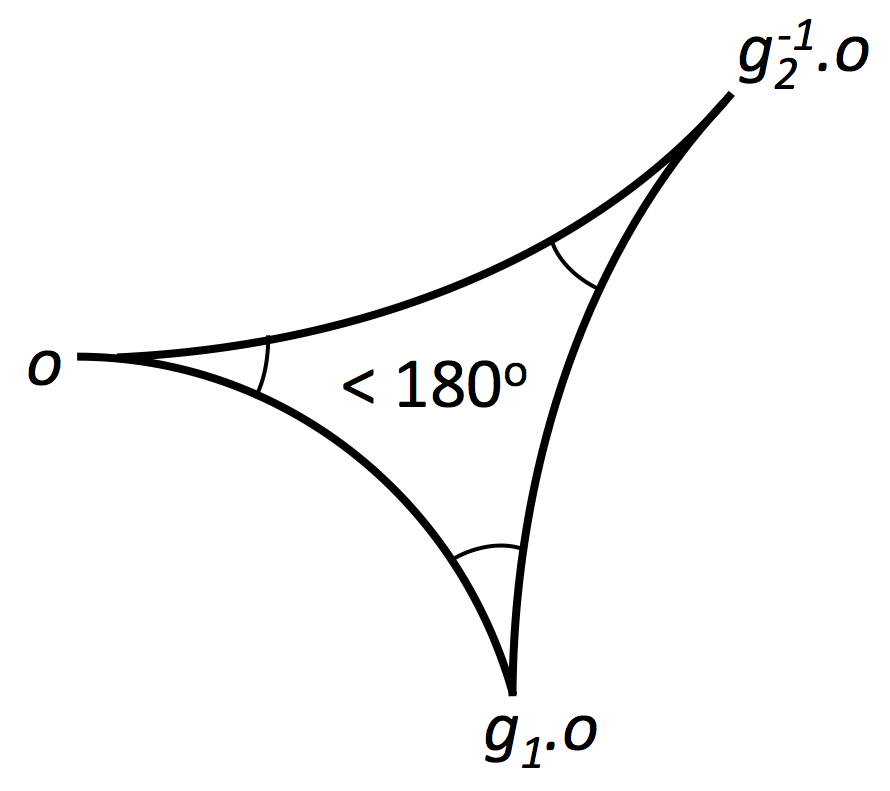
Figure 1. Hyperbolic triangle

Noncommutative T-duality at the level of $K$-theory groups is the composition,

$$T_{\Sigma_{g}}=\mu_{\theta}\circ PD_{\Sigma_{g}}\colon K^{0}(\Sigma_{g})\stackrel{{\scriptstyle\sim}}{{\longrightarrow}}K_{0}(C^{*}_{r}(\Gamma_{g},\sigma)).$$

By Eq. (3.2) and Proposition 3.1, we have

Corollary 3.2.

$T_{\Sigma_{g}}$ exchanges $[{\bf 1}_{\Sigma_{g}}]\leftrightarrow[\mathcal{P}_{\sigma}]$ and $[\widetilde{\mathcal{L}}]\leftrightarrow[\bf 1]$.

Remark 3.3.

From the physical perspective, $\tau$ is relevant for gap-labelling problems, while the geometrically defined 2-cocycle $\tau_{c}$ turns out to be cohomologous to the (hyperbolic) Kubo conductivity cocycle $\tau_{K}$ [17] which computes the contribution to the Hall conductance by a projection $\mathcal{P}$. Thus $[\mathcal{P}_{\sigma}]$ has the physical meaning of the $K$-theory class contributing to the smallest nonzero value of the quantised Hall conductance.

Remark 3.4.

In the Euclidean case where $\Gamma={\mathbb{Z}}^{2}$ and $C^{*}_{r}({\mathbb{Z}}^{2},\sigma)$ is the noncommutative torus, $\mathcal{P}_{\sigma}$ is the Rieffel projection, cf. [53].

3.2. Noncommutative T-duality for $\Sigma_{g,\nu}$ in even degree

When ${\bm{\nu}}$ is nonempty, we need to consider the orbifold $K$-theory $K^{0}_{\rm orb}(\Sigma_{g,{\bm{\nu}}})\cong K^{0}_{G}(\Sigma_{g^{\prime}})$. Note that for the smooth manifold $\Sigma_{g}$, we have $K^{0}_{\rm orb}(\Sigma_{g})=K^{0}(\Sigma_{g})$. Returning to $\Sigma_{g,{\bm{\nu}}}$, besides the trivial line bundle ${\bf 1}_{\Sigma_{g,{\bm{\nu}}}}$ and the (virtual) line bundle $\widetilde{\mathcal{L}}$ whose Chern class generates the top degree cohomology, there are new orbifold line bundles on $\Sigma_{g,{\bm{\nu}}}$ (or $G$-equivariant bundles on $\Sigma_{g^{\prime}}$) which generate extra copes of ${\mathbb{Z}}$ in $K^{0}_{\rm orb}(\Sigma_{g,{\bm{\nu}}})$. These extra bundles can be labelled by the non-trivial characters $\chi_{j}$ of ${\mathbb{Z}}_{\nu_{j}}$ at each singular point $p_{j}$ [43]. We write $\widetilde{\mathcal{L}}_{\chi_{j}}$ for these virtual bundles, and there are $\sum_{j=1}^{r}(\nu_{j}-1)$ classes of them. Then $[{\bf 1}_{\Sigma_{g,{\bm{\nu}}}]},[\widetilde{\mathcal{L}}]$ and $[\widetilde{\mathcal{L}}_{\chi_{j}}],j=1,\ldots,r$ account for

$$K^{0}_{\rm orb}(\Sigma_{g,{\bm{\nu}}})\cong{\mathbb{Z}}^{2+\sum_{j=1}^{r}(\nu_{j}-1)}.$$

Poincaré duality $PD_{\Sigma_{g,{\bm{\nu}}}}$ takes $[\mathcal{E}]\in K^{0}_{\rm orb}(\Sigma_{g,{\bm{\nu}}})$ to the class of the $\mathcal{E}$-twisted Dirac operator (denoted $/\!\!\!\partial_{\mathcal{E}}^{+}$ in [44]) in $K^{\rm orb}_{0}(\Sigma_{g,{\bm{\nu}}})\cong K_{0}^{\Gamma_{g,{\bm{\nu}}}}(\underline{E}\Gamma_{g,{\bm{\nu}}})$ with the latter isomorphism given by lifting $/\!\!\!\partial_{\mathcal{E}}^{+}$ to a $\Gamma_{g,{\bm{\nu}}}$-invariant operator $\widetilde{/\!\!\!\partial_{\mathcal{E}}^{+}}$ on the contractible cover ${\mathbb{H}}\simeq\underline{E}\Gamma_{g,{\bm{\nu}}}$. Recall also that the twisted Baum–Connes assembly map $\mu_{\theta}$ gives an isomorphism

$$\mu_{\theta}:K_{0}^{\Gamma_{g,{\bm{\nu}}}}(\underline{E}\Gamma_{g,{\bm{\nu}}})\rightarrow K_{0}(C^{*}_{r}(\Gamma_{g,{\bm{\nu}}},\sigma)),$$

which is in accordance with Eq. (2.5). Noncommutative T-duality in this case is the map $T_{\Sigma_{g,{\bm{\nu}}}}=\mu_{\theta}\circ PD_{\Sigma_{g,{\bm{\nu}}}}$, where

$$T_{\Sigma_{g,{\bm{\nu}}}}:K^{0}_{\rm orb}(\Sigma_{g,{\bm{\nu}}})\ni[\mathcal{E}]\mapsto{\rm index}_{C^{*}_{r}(\Gamma_{g,{\bm{\nu}}},\sigma)}(/\!\!\!\partial_{\mathcal{E}}^{+}\otimes\mathcal{V}_{\sigma})\in K_{0}(C^{*}_{r}(\Gamma_{g,{\bm{\nu}}},\sigma)).$$

There is again a higher index formula [43, 44]

$$\tau_{c}(T_{\Sigma_{g,{\bm{\nu}}}}([\mathcal{E}]))=\phi\,{\rm rank}(\mathcal{E}),$$ (3.3)

where $\phi=2(g-1)+(r-\nu)\in{\mathbb{Q}}$ is the orbifold Euler characteristic of $\Sigma_{g,{\bm{\nu}}}$. Let $[\mathcal{P}_{\sigma}]\in K_{0}(C^{*}_{r}(\Gamma_{g,{\bm{\nu}}},\sigma))$ be a generator such that $\tau_{c}(\mathcal{P}_{\sigma})=\phi$. Then we have

Corollary 3.5.

$T_{\Sigma_{g,{\bm{\nu}}}}$ takes $[\widetilde{\mathcal{L}}],[\widetilde{\mathcal{L}}_{\chi_{j}}]$ into ${\rm ker}\,\tau_{c}$, and $[{\bf 1}_{\Sigma_{g,{\bm{\nu}}}}]\mapsto[\mathcal{P}_{\sigma}]$ up to an element in ${\rm ker}\,\tau_{c}$.

Note that Corollary 3.5 is consistent with the special case in Corollary 3.2.

3.3. Noncommutative T-duality for $\Sigma_{g,\nu}$ in odd degree

For the T-duality isomorphism $K^{-1}_{\rm orb}(\Sigma_{g,{\bm{\nu}}})\leftrightarrow K_{1}(C^{*}_{r}(\Gamma_{g,{\bm{\nu}}}))$, it is convenient to identify both the $K$-groups with ${\mathbb{Z}}^{2g}$ in terms of the canonical $2g$ group generators $A_{i},B_{i}$ of $\Gamma_{g,{\bm{\nu}}}$.

First, consider the torsion free case where ${\bm{\nu}}$ is empty. The abelianisation of $\Gamma_{g}$ is $\Gamma_{g}^{\rm ab}\cong{\mathbb{Z}}^{2g}={\mathbb{Z}}^{g}\oplus{\mathbb{Z}}^{g}$ with canonical generators denoted $A_{i}^{\rm ab},B_{i}^{\rm ab}$, and we can also identify $\Gamma_{g}^{\rm ab}\cong H_{1}(\Gamma_{g},{\mathbb{Z}})\cong H_{1}(\Sigma_{g})$ with the generating cycles of the latter denoted $l_{A_{i}},l_{B_{i}}$. More generally, $Y^{\rm ab}\in\Gamma_{g}^{\rm ab}$ has a corresponding homology class $[l_{Y^{\rm ab}}]\in H_{1}(\Sigma_{g})$.

Let $L^{\sigma}_{Y}$ denote $\sigma$-left translation by $Y\in\Gamma_{g}$, which is a unitary in $C^{*}_{r}(\Gamma_{g},\sigma)$. The inclusion $Y\mapsto L^{\sigma}_{Y}$ induces a homomorphism $\widetilde{\beta}_{a}^{\sigma}:\Gamma_{g}\rightarrow K_{1}(C^{*}_{r}(\Gamma_{g},\sigma))$ which factors through

$$\beta_{a}^{\sigma}:\Gamma_{g}^{\rm ab}\rightarrow K_{1}(C^{*}_{r}(\Gamma_{g},\sigma)).$$

In fact, $\beta_{a}^{\sigma}$ is an isomorphism here, so that $[L_{A_{i}}^{\sigma}],[L_{B_{i}}^{\sigma}]$ are canonical generators for $K_{1}(C^{*}_{r}(\Gamma_{g},\sigma))$ [48] (in the untwisted case the rational injectivity of $\beta_{a}$ is a general result of [25, 2]). There is also a canonical homomorphism

$$\beta_{t}:\Gamma_{g}^{\rm ab}\rightarrow K_{1}(\Sigma_{g})$$

such that

$$\beta_{a}^{\sigma}=\mu_{\theta}\circ\beta_{t}$$ (3.4)

where $\mu_{\theta}=\mu_{\theta}^{\Gamma_{g}}$ is the twisted Baum–Connes assembly map $K_{1}(B\Gamma_{g}\simeq\Sigma_{g})\rightarrow K_{1}(C^{*}_{r}(\Gamma_{g},\sigma))$ [61, 48]. It is convenient to identify $K_{1}(\Sigma_{g})$ with $H_{1}(\Gamma_{g})$ under the Chern character, then $\beta_{t}(Y^{\rm ab})$ corresponds to $[l_{Y^{\rm ab}}]$.

When ${\bm{\nu}}$ is nonempty, $\Gamma_{g,{\bm{\nu}}}^{\rm ab}$ may have torsion elements but its free part is still ${\mathbb{Z}}^{2g}$ and generated by $A_{i}^{\rm ab},B_{i}^{\rm ab}$ as before. Rationally, $\beta_{a}^{\sigma}:\Gamma_{g,{\bm{\nu}}}^{\rm ab}\rightarrow K_{1}(C^{*}_{r}(\Gamma_{g,{\bm{\nu}}},\sigma))$ still gives an isomorphism, so $K_{1}(C^{*}_{r}(\Gamma_{g},\sigma))$ is again generated by $[L_{A_{i}}^{\sigma}],[L_{B_{i}}^{\sigma}]$. In particular, $[L_{Y}^{\sigma}]$ depends only on $Y^{\rm ab}$. The Baum–Connes map is

$$\mu_{\theta}=\mu_{\theta}^{\Gamma_{g,{\bm{\nu}}}}:K_{1}^{\rm orb}(\Sigma_{g,{\bm{\nu}}})=K_{1}^{G}(\Sigma_{g^{\prime}})\rightarrow K_{1}(C^{*}_{r}(\Gamma_{g},\sigma)),$$

and the homomorphism $\beta_{t}:\Gamma_{g,{\bm{\nu}}}^{\rm ab}\rightarrow K_{1}^{\rm orb}(\Sigma_{g,{\bm{\nu}}})$ is such that Eq. (3.4) holds. In particular, $\beta_{t}$ vanishes on the torsion elements of $\Gamma_{g,{\bm{\nu}}}^{\rm ab}$ [61]. Using the Baum–Connes Chern character [4] or delocalised equivariant homology [43], we may identify $K_{1}^{\rm orb}(\Sigma_{g,{\bm{\nu}}})\cong H_{1}(\Sigma_{g,{\bm{\nu}}})\cong{\mathbb{Z}}^{2g}$ with the generating cycles $l_{A_{i}},l_{B_{i}}$ as before. Note that torsion elements of $\Gamma_{g,{\bm{\nu}}}^{\rm ab}$ such as $C_{j}$ do not contribute any nontrivial ($K$)-cycles.

With these descriptions, we can now state the effect of the noncommutative T-duality map

$$T_{\Sigma_{g,{\bm{\nu}}}}:K^{-1}_{\rm orb}(\Sigma_{g,{\bm{\nu}}})\rightarrow K_{1}(C^{*}_{r}(\Gamma_{g,{\bm{\nu}}},\sigma)),$$

defined as $\mu_{\theta}$ composed with Poincaré duality, as follows.

Proposition 3.6.

Let $[U]\in K^{-1}_{\rm orb}(\Sigma_{g,{\bm{\nu}}})$ have Chern character whose Poincaré dual is $[l_{Y^{\rm ab}}]$, then $T_{\Sigma_{g,{\bm{\nu}}}}([U])=[L_{Y}^{\sigma}]\in K_{1}(C^{*}_{r}(\Gamma_{g,{\bm{\nu}}},\sigma))$.

Note that if $[U]$ is nontrivial, $Y$ is necessarily torsion free. Also, the intersection pairing qof cycles is such that $[l_{A_{i}}]\#[l_{B_{j}}]=\delta_{ij}$ so that the Poincaré duals can be described explicitly. For example, the Poincaré dual of $[l_{A_{i}}]$ evaluates to 1 on $[l_{B_{i}}]$ and kills the other generating cycles; e.g. this can be seen from Fig. 3.

4. Bulk-boundary maps

4.1. Preliminaries: UCT and extensions

The classical index theorem linking the Fredholm index of a Toeplitz operator with the winding number of its symbol may be understood in terms of $K$-theory and extensions as follows. We think of $C({\mathbb{T}})\cong C^{*}_{r}({\mathbb{Z}})$ acting on $l^{2}({\mathbb{Z}})\cong L^{2}({\mathbb{T}})$ so that $C({\mathbb{T}})$ is generated by translations $L_{n},$ $n\in{\mathbb{Z}}$ whose Fourier transforms are multiplication by $e^{{\rm i}n\theta}$. When truncated to Hardy space thought of as $l^{2}({\mathbb{N}})$, the translation operator $L_{1}$ becomes a unilateral shift $\widetilde{L}_{1}$, and acquires a dimension 1 cokernel (the subspace for the boundary $n=0$). It is a Fredholm operator $\widetilde{L}_{1}=T_{f}$ with invertible symbol $f=e^{{\rm i}\theta}$ and index$(T_{f})=-1=-{\rm Wind}(f)$. The Toeplitz algebra $\mathcal{T}$ generated by $\widetilde{L}_{1}$ is a non-split extension

$$1\longrightarrow\mathcal{K}\longrightarrow\mathcal{T}\overset{\small\rm symbol}{\longrightarrow}C({\mathbb{T}})\longrightarrow 1.$$ (4.1)

with kernel $\mathcal{K}$ the compact operators on $l^{2}({\mathbb{N}})$. In the seminal work of Brown–Douglas–Fillmore (BDF) [16], the extension theory of $C^{*}$-algebras $\mathcal{A}$ by $\mathcal{K}$ (denoted ${\rm Ext}(C(X))$ up to a certain notion of equivalence) was shown to be related to $K$-homology in the sense that ${\rm Ext}(C(X))\cong K_{1}(X)$ (at least when $X$ is a CW complex). From this point of view, Eq. (4.1) defines the generating element of $K_{1}({\mathbb{T}})$, and the analytic index pairing $K_{1}({\mathbb{T}})\times K^{-1}({\mathbb{T}})\rightarrow K_{0}(\mathcal{K})\cong{\mathbb{Z}}$ taking $([\mathcal{T}],[f])\mapsto{\rm Index}(T_{f})$ realises the topological winding number/index of the symbol $f$ (up to a sign).

As explained in the latter part of this section, we will need to consider extensions of $C^{*}_{r}(\Gamma,\sigma)$ by $C({\mathbb{T}})$ (actually its stabilisation), where $\Gamma=\Gamma_{g,{\bm{\nu}}}$, in order to model bulk-boundary maps. Such extensions may be studied using the universal coefficient theorem (UCT) due to Rosenberg–Schochet [58], and vastly generalises the BDF theory. By Corollary 7.2 in [58], $\mathcal{K}\rtimes\Gamma\cong C^{*}_{r}(\Gamma,\sigma)\otimes\mathcal{K}$ satisfies UCT, so that one has a short exact sequence,

$$0\to {\rm Ext}^{1}_{\mathbb{Z}}(K_{*}(C^{*}_{r}(\Gamma,\sigma)),K_{*}(C({\mathbb{T}})))\to KK^{1}(C^{*}_{r}(\Gamma,\sigma),C({\mathbb{T}}))\to$$

$$\to{\rm Hom}(K_{1}(C^{*}_{r}(\Gamma,\sigma)),K_{0}(C({\mathbb{T}})))\oplus{\rm Hom}(K_{0}(C^{*}_{r}(\Gamma,\sigma)),K_{1}(C({\mathbb{T}})))\to 0.$$

Since $K_{*}(C^{*}_{r}(\Gamma,\sigma))$ for $\Gamma=\Gamma_{g,{\bm{\nu}}}$ and $K_{*}(C({\mathbb{T}}))$ are free abelian groups, ${\rm Ext}^{1}_{\mathbb{Z}}=0$, therefore

$$KK^{1}(C^{*}_{r}(\Gamma,\sigma),C({\mathbb{T}})) \cong$$

$${\rm Hom}(K_{1}(C^{*}_{r}(\Gamma,\sigma)), K_{0}(C({\mathbb{T}})))\oplus{\rm Hom}(K_{0}(C^{*}_{r}(\Gamma,\sigma)),K_{1}(C({\mathbb{T}}))).$$

This shows that any element $\alpha\oplus\partial$ of the RHS above determines a unique extension class [35, 11]

$$0\to C({\mathbb{T}})\otimes\mathcal{K}\to E(\alpha\oplus\partial)\to C^{*}_{r}(\Gamma,\sigma)\to 0$$

giving rise to the 6-term exact sequence in K-theory, with boundary maps

$$\alpha:K_{1}(C^{*}_{r}(\Gamma,\sigma))\to K_{0}(C({\mathbb{T}}))$$

$$\partial:K_{0}(C^{*}_{r}(\Gamma,\sigma))\to K_{1}(C({\mathbb{T}})).$$

4.2. Bulk-boundary maps in Euclidean space

In [38, 56] a model for bulk-boundary maps was introduced, in which a bulk $C^{*}$-algebra was extended by a boundary $C^{*}$-algebra, and the resulting boundary homomorphisms in $K$-theory taken to be bulk-boundary maps. This was applied successfully to prove equality of bulk and boundary conductivities in the physical context of the Integer quantum Hall effect. In the cases studied there, the bulk algebra is generated by a lattice ${\mathbb{Z}}^{2}$ of Euclidean magnetic translation symmetries generated by elements $A,B$, while the boundary symmetries comprised only the subgroup ${\mathbb{Z}}_{A}$ generated by $A$ which translated along the physical codimension-1 boundary (a Euclidean line containing a ${\mathbb{Z}}_{A}$ orbit which partitions Euclidean space into the “bulk” on one side and the “vacuum” on the other). The extension was taken to be a Toeplitz-like extension (in the sense of Pimsner–Voiculescu [54]) with the effect of imposing boundary conditions on the bulk translations operators. Then the bulk-boundary map was (ignoring the modelling of disorder)

$$\partial_{\rm PV}:K_{0}(C^{*}_{r}({\mathbb{Z}}^{2},\sigma))\rightarrow K_{1}(C^{*}_{r}({\mathbb{Z}}_{A}))=K_{1}(C({\mathbb{T}})),$$

which mapped the class of the Rieffel projection $[\mathcal{P}_{\sigma}]$ to the generator of $K_{1}(C({\mathbb{T}}))$ and mapped the trivial projection [1] to zero. Similarly, under $\alpha_{\rm PV}:K_{1}(C^{*}_{r}({\mathbb{Z}}^{2},\sigma))\rightarrow K_{0}(C^{*}_{r}({\mathbb{Z}}_{A}))$, the class of the unitary $[L_{B}]$ maps to the generator whereas $[L_{A}]$ maps to zero. An explicit analysis of $\partial_{\rm PV}$ as a Kasparov product with the class of the above extension in $KK^{1}(C^{*}_{r}({\mathbb{Z}}^{2},\sigma),C({\mathbb{T}}))$ was carried out in [12].

4.3. Bulk-boundary maps in the hyperbolic plane

For our hyperbolic plane generalisation, the bulk-algebra is taken to be $C^{*}_{r}(\Gamma,\sigma)$ as discussed in Section 2, and we need a sensible notion of a “boundary” in ${\mathbb{H}}$ and translations therein. A natural choice is to take the subgroup ${\mathbb{Z}}_{X}$ generated by some hyperbolic element (necessarily non-torsion) $X\in\Gamma$, and the boundary algebra to be $C^{*}_{r}({\mathbb{Z}}_{X})\cong C({\mathbb{T}})$. The geometric meaning is as follows [33, 6].

Any hyperbolic transformation $X$ of ${\mathbb{H}}$ has two idealised fixed points at infinity (they are two points on the boundary circle in the Poincaré disc model of ${\mathbb{H}}$). There is a unique geodesic (hyperbolic straight line), called the axis of $X$, connecting these fixed points. A hypercycle for $X$ comprises the points in ${\mathbb{H}}$ which are on one side of and a fixed hyperbolic distance away from the geodesic. Thus all the hypercycles for $X$ only intersect (eventually) at the two fixed points — a manifestation of the non-Euclidean geometry. The orbit of a given point in ${\mathbb{H}}$ under ${\mathbb{Z}}_{X}$ is contained in a hypercycle for $X$ through that point, and will serve as a boundary partitioning ${\mathbb{H}}$ into two sides (Fig. 2).

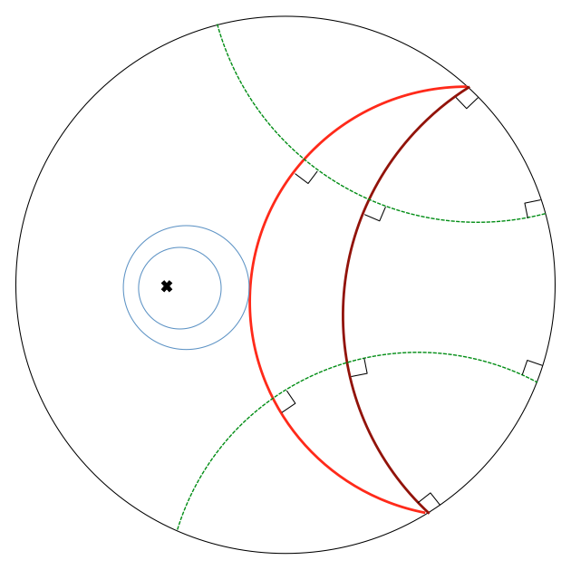
Figure 2. In the Poincaré disk model of the hyperbolic plane, geodesics (green) are arcs of (Euclidean) circles that orthogonally intersect the boundary circle at infinity. A hyperbolic transformation effects translations along hypercycles (red) connecting its two idealised fixed points at infinity. One such hypercycle is a geodesic (dark red). An elliptic transformation effects “rotations” about some fixed point $\times$, and each of its orbits lies in a hyperbolic circle (blue).

Note that such a “boundary hypercycle” is homeomorphic to ${\mathbb{R}}$, and in the quotient ${\mathbb{H}}/\Gamma=\Sigma$ it becomes a cycle $l_{X}:S^{1}={\mathbb{R}}/{\mathbb{Z}}_{X}\rightarrow\Sigma$. Recall that under the identification ${\mathbb{Z}}^{2g}\cong H_{1}(\Sigma)$, the homology classes are labelled by $[l_{X^{\rm ab}}]$ with $X^{\rm ab}\in\Gamma^{\rm ab}$, and we see that $[l_{X}]=[l_{X^{\rm ab}}]$. The intersection pairing is $[l_{A_{i}}]\#[l_{B_{j}}]=\delta_{ij}$, which means that we can interpret $B_{i}$ as a translation transverse to boundaries generated along $A_{i}$, while for $j\neq i$, the translations $A_{j},B_{j}$ are not transversal (their orbits cross the boundary an equal number of times in each direction). The geometry of intersections of hypercycles is illustrated for the special case of $\Gamma_{g=2}$ in Fig. 3.

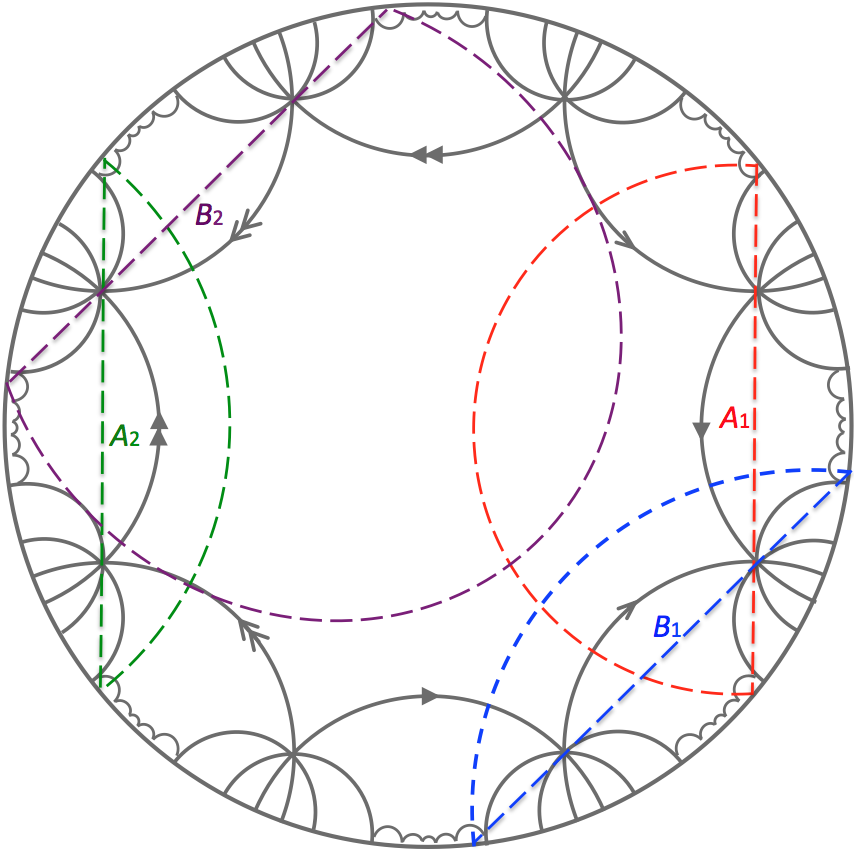
Figure 3. A tiling of the Poincaré disk by fundamental polygons for $\Gamma_{g}$ with $g=2$ (edges near the boundary circle are omitted to reduce clutter). The vertices of the polygons constitute a Cayley graph for $\Gamma_{g}$. The edges of the central octagon are pairwise identified according to the arrows to form the Riemann surface $\Sigma_{g}$. For each of the hyperbolic generators $A_{1},B_{1},A_{2},B_{2}$ of $\Gamma_{2}$, two hypercycles are drawn (dashed lines). We see that $(A_{i},B_{i})$ are transversal to each other for $i=1$ and also $i=2$, but the other pairs are not. For instance, although the large $B_{2}$ hypercycle intersects the large $A_{1}$ hypercycle twice in total, their signed intersection number is $0$.

Recall that $K_{0}(C^{*}_{r}(\Gamma))\cong{\mathbb{Z}}[\mathcal{P}_{\sigma}]\oplus{\rm ker}\,\tau_{c}$ where we had distinguished ${\mathbb{Z}}[\mathcal{P}_{\sigma}]$ as the classes that contribute to Hall conductance in Proposition 3.1 and Remark 3.3. Also, we explained in Section 3.3 that $K_{1}(C^{*}_{r}(\Gamma,\sigma))\cong{\mathbb{Z}}^{2g}$ with all classes realisable by $[L_{Y^{\rm ab}}^{\sigma}]$ for some $Y^{\rm ab}\in\Gamma^{\rm ab}$. Guided by the geometry of the hypercyclic boundary defined by $X$ and the bulk-boundary map in the Euclidean case, we will define

$$\partial_{X}([\mathcal{P}_{\sigma}])=[\zeta],\qquad\partial_{X}({\rm ker}\,\tau_{c})=0,$$ (4.2)

where $[\zeta]$ is the generator of $K_{1}(C({\mathbb{T}}))\cong K^{-1}({\mathbb{T}})\cong{\mathbb{Z}}$, and

$$\alpha_{X}([L_{Y}^{\sigma}])=\alpha_{X}([L_{Y^{\rm ab}}^{\sigma}])=([l_{Y^{\rm ab}}]\#[l_{X^{\rm ab}}])\cdot[{\bf 1}].$$ (4.3)

The intuition behind Eq. (4.3) is that each translation transverse to the boundary gets modified to a “half-translation” and leaves behind a zero mode. This is analogous to the interpretation of the classical Fredholm index of the unilateral shift operator on ${\mathbb{N}}$. Eq. (4.2) generalises the Euclidean case, with the only change being that the extra non-trivial classes in $K_{0}(C^{*}_{r}(\Gamma,\sigma))$, which are due to the conical singularities $p_{j}$, are mapped to zero under $\partial_{X}$. This is reasonable since the boundary hypercycle is not generally preserved by the elliptic symmetries $C_{j}$ so it cannot “see” the $K$-theory classes arising from them.

Through the UCT, the combination $\alpha_{X}\oplus\partial_{X}$ specifies (albeit abstractly) the class of an extension of $C^{*}_{r}(\Gamma_{g,{\bm{\nu}}},\sigma)$ by $C^{*}_{r}({\mathbb{Z}}_{X})\cong C({\mathbb{T}})$, generalising the Toeplitz-like extension used in the Euclidean case. The sign ambiguity in $[\zeta]$ corresponds to the choice of side of the boundary to take as the bulk; notice that the induced orientation on the boundary depends on this choice.

4.4. T-duality simplifies the bulk-boundary correspondence

A hypercyclic boundary containing an orbit of ${\mathbb{Z}}_{X}$ gives rise to a cycle $l_{X}:S^{1}\rightarrow\Sigma$, and there is a pullback $l_{X}^{*}$ in $K$-theory which we can think of as a “restriction map” to the immersed image of $l_{X}$. When we regard the boundary as ${\mathbb{R}}\simeq E{\mathbb{Z}}_{X}$, then the quotient under ${\mathbb{Z}}_{X}$ is $S^{1}={\mathbb{R}}/{\mathbb{Z}}_{X}\simeq B{\mathbb{Z}}_{X}$, and we can apply T-duality (3.1) to this circle.

Theorem 4.1.

The following diagram commutes for $\bullet=0,1$,

$$\lx@xy@svg{\hbox{\raise 0.0pt\hbox{\kern 17.64722pt\hbox{\ignorespaces\ignorespaces\ignorespaces\hbox{\vtop{\kern 0.0pt\offinterlineskip\halign{\entry@#!@&&\entry@@#!@\cr&\\&\crcr}}}\ignorespaces{\hbox{\kern-16.50418pt\raise 0.0pt\hbox{\hbox{\kern 0.0pt\raise 0.0pt\hbox{\hbox{\kern 3.0pt\raise 0.0pt\hbox{$\textstyle{K^{\bullet}_{\rm orb}(\Sigma)\ignorespaces\ignorespaces\ignorespaces\ignorespaces\ignorespaces\ignorespaces\ignorespaces\ignorespaces}$}}}}}}}\ignorespaces\ignorespaces\ignorespaces\ignorespaces{}{\hbox{\lx@xy@droprule}}\ignorespaces\ignorespaces\ignorespaces{\hbox{\kern 0.0pt\raise-20.44345pt\hbox{{}\hbox{\kern 0.0pt\raise 0.0pt\hbox{\hbox{\kern 3.0pt\hbox{\hbox{\kern 0.0pt\raise-2.2125pt\hbox{$\scriptstyle{l_{X}^{*}}$}}}\kern 3.0pt}}}}}}\ignorespaces{\hbox{\kern 0.0pt\raise-29.24916pt\hbox{\hbox{\kern 0.0pt\raise 0.0pt\hbox{\lx@xy@tip{1}\lx@xy@tip{-1}}}}}}{\hbox{\lx@xy@droprule}}{\hbox{\lx@xy@droprule}}\ignorespaces\ignorespaces\ignorespaces\ignorespaces{}{\hbox{\lx@xy@droprule}}\ignorespaces\ignorespaces\ignorespaces{\hbox{\kern 29.98235pt\raise 4.28406pt\hbox{{}\hbox{\kern 0.0pt\raise 0.0pt\hbox{\hbox{\kern 3.0pt\hbox{\hbox{\kern 0.0pt\raise-1.28406pt\hbox{$\scriptstyle{\sim}$}}}\kern 3.0pt}}}}}}\ignorespaces\ignorespaces\ignorespaces{\hbox{\kern 28.72871pt\raise-6.075pt\hbox{{}\hbox{\kern 0.0pt\raise 0.0pt\hbox{\hbox{\kern 3.0pt\hbox{\hbox{\kern 0.0pt\raise-1.70833pt\hbox{$\scriptstyle{T_{\Sigma}}$}}}\kern 3.0pt}}}}}}\ignorespaces{\hbox{\kern 41.64722pt\raise 0.0pt\hbox{\hbox{\kern 0.0pt\raise 0.0pt\hbox{\lx@xy@tip{1}\lx@xy@tip{-1}}}}}}{\hbox{\lx@xy@droprule}}{\hbox{\lx@xy@droprule}}{\hbox{\kern 41.64722pt\raise 0.0pt\hbox{\hbox{\kern 0.0pt\raise 0.0pt\hbox{\hbox{\kern 3.0pt\raise 0.0pt\hbox{$\textstyle{K_{\bullet}(C^{*}_{r}(\Gamma,\sigma))\ignorespaces\ignorespaces\ignorespaces\ignorespaces}$}}}}}}}\ignorespaces\ignorespaces\ignorespaces\ignorespaces{}{\hbox{\lx@xy@droprule}}\ignorespaces\ignorespaces\ignorespaces{\hbox{\kern 71.40915pt\raise-20.44345pt\hbox{{}\hbox{\kern 0.0pt\raise 0.0pt\hbox{\hbox{\kern 3.0pt\hbox{\hbox{\kern 0.0pt\raise-1.74722pt\hbox{$\scriptstyle{\partial_{X}}$}}}\kern 3.0pt}}}}}}\ignorespaces{\hbox{\kern 71.40915pt\raise-29.24916pt\hbox{\hbox{\kern 0.0pt\raise 0.0pt\hbox{\lx@xy@tip{1}\lx@xy@tip{-1}}}}}}{\hbox{\lx@xy@droprule}}{\hbox{\lx@xy@droprule}}{\hbox{\kern-17.64722pt\raise-40.88692pt\hbox{\hbox{\kern 0.0pt\raise 0.0pt\hbox{\hbox{\kern 3.0pt\raise 0.0pt\hbox{$\textstyle{K^{\bullet}(S^{1})\ignorespaces\ignorespaces\ignorespaces\ignorespaces}$}}}}}}}\ignorespaces\ignorespaces\ignorespaces\ignorespaces{}{\hbox{\lx@xy@droprule}}\ignorespaces\ignorespaces\ignorespaces{\hbox{\kern 29.98235pt\raise-36.60286pt\hbox{{}\hbox{\kern 0.0pt\raise 0.0pt\hbox{\hbox{\kern 3.0pt\hbox{\hbox{\kern 0.0pt\raise-1.28406pt\hbox{$\scriptstyle{\sim}$}}}\kern 3.0pt}}}}}}\ignorespaces\ignorespaces\ignorespaces{\hbox{\kern 25.61206pt\raise-46.97302pt\hbox{{}\hbox{\kern 0.0pt\raise 0.0pt\hbox{\hbox{\kern 3.0pt\hbox{\hbox{\kern 0.0pt\raise-1.69722pt\hbox{$\scriptstyle{T_{\rm circle}}$}}}\kern 3.0pt}}}}}}\ignorespaces{\hbox{\kern 52.57164pt\raise-40.88692pt\hbox{\hbox{\kern 0.0pt\raise 0.0pt\hbox{\lx@xy@tip{1}\lx@xy@tip{-1}}}}}}{\hbox{\lx@xy@droprule}}{\hbox{\lx@xy@droprule}}{\hbox{\kern 52.57164pt\raise-40.88692pt\hbox{\hbox{\kern 0.0pt\raise 0.0pt\hbox{\hbox{\kern 3.0pt\raise 0.0pt\hbox{$\textstyle{K^{\bullet-1}({\mathbb{T}})}$}}}}}}}\ignorespaces}}}}\ignorespaces. \textstyle{K^{\bullet}_{\rm orb}(\Sigma)\ignorespaces\ignorespaces\ignorespaces\ignorespaces\ignorespaces\ignorespaces\ignorespaces\ignorespaces} \scriptstyle{l_{X}^{*}} \scriptstyle{\sim} \scriptstyle{T_{\Sigma}} \textstyle{K_{\bullet}(C^{*}_{r}(\Gamma,\sigma))\ignorespaces\ignorespaces\ignorespaces\ignorespaces} \scriptstyle{\partial_{X}} \textstyle{K^{\bullet}(S^{1})\ignorespaces\ignorespaces\ignorespaces\ignorespaces} \scriptstyle{\sim} \scriptstyle{T_{\rm circle}} \textstyle{K^{\bullet-1}({\mathbb{T}})} \textstyle{K^{\bullet}_{\rm orb}(\Sigma)\ignorespaces\ignorespaces\ignorespaces\ignorespaces\ignorespaces\ignorespaces\ignorespaces\ignorespaces} \scriptstyle{l_{X}^{*}} \scriptstyle{\sim} \scriptstyle{T_{\Sigma}} \textstyle{K_{\bullet}(C^{*}_{r}(\Gamma,\sigma))\ignorespaces\ignorespaces\ignorespaces\ignorespaces} \scriptstyle{\partial_{X}} \textstyle{K^{\bullet}(S^{1})\ignorespaces\ignorespaces\ignorespaces\ignorespaces} \scriptstyle{\sim} \scriptstyle{T_{\rm circle}} \textstyle{K^{\bullet-1}({\mathbb{T}})}$$

Proof.

We check this by computing the maps on generators of $K^{\bullet}_{\rm orb}(\Sigma)$. For $\bullet=0$, since $S^{1}$ is one dimensional, it is clear that only the rank invariant survives under $l_{X}^{*}$. We compute

$$T_{\rm circle}\circ l_{X}^{*}([{\bf 1}]_{\Sigma})=T_{\rm circle}([{\bf 1}]_{S^{1}})=[\zeta]$$

By Corollaries 3.2, 3.5, and the formula for $\partial_{X}$ in Eq. (4.2), we also have

$$\partial_{X}\circ T_{\Sigma}([{\bf 1}]_{\Sigma})=\partial_{X}([\mathcal{P}_{\sigma}])=[\zeta].$$

As for the other generators $[\widetilde{\mathcal{L}}],[\widetilde{\mathcal{L}}_{\chi_{j}}]$ of $K^{0}_{\rm orb}(\Sigma)$, they are mapped to zero by $l_{X}^{*}$ (and thus by $T_{\rm circle}\circ l_{X}^{*}$), while $T_{\Sigma}$ takes them to ${\rm ker}\,\tau_{c}$ which vanishes under $\partial_{X}$.

For $\bullet=1$, let $[U]\in K^{-1}_{\rm orb}(\Sigma)$ have Chern character ${\rm Ch}([U])$ Poincaré dual to $[l_{Y^{\rm ab}}]$, and $[W]$ be a generator of $K^{-1}(S^{1})$. We compute

$$\langle{\rm Ch}(l_{X}^{*}[U]),[S^{1}]\rangle =\langle{l_{X}^{*}\rm Ch}([U]),[S^{1}]\rangle$$

$$=\langle{\rm PD}([l_{Y^{\rm ab}}]),(l_{X})_{*}([S^{1}])\rangle$$

$$=\langle{\rm PD}([l_{Y^{\rm ab}}]),[l_{X^{\rm ab}}]\rangle$$

$$=[l_{Y^{\rm ab}}]\#[l_{X^{\rm ab}}]$$

$$=\langle[l_{Y^{\rm ab}}]\#[l_{X^{\rm ab}}]\cdot[W],[S^{1}]\rangle,$$

which combined with Eq. (3.1) gives

$$T_{\rm circle}\circ l_{X}^{*}([U])=T_{\rm circle}(([l_{X^{\rm ab}}]\#[l_{Y^{\rm ab}}])\cdot[W])=[l_{X^{\rm ab}}]\#[l_{Y^{\rm ab}}]\cdot[{\bf 1}]$$

On the other hand, using Proposition 3.6 we also get

$$\alpha_{X}\circ T_{\Sigma}([U])=\alpha_{X}([L_{Y}^{\sigma}])=[l_{X^{\rm ab}}]\#[l_{Y^{\rm ab}}]\cdot[{\bf 1}].$$

∎

To summarise, the relatively complicated and abstract boundary map,

$$\alpha_{X}\oplus\partial_{X}\colon K_{*}(C^{*}_{r}(\Gamma,\sigma))\to K^{*-1}({\mathbb{T}})$$

is equivalent to the conceptually simple geometric restriction-to-boundary maps,

$$l_{X}^{*}\colon K^{\bullet}_{\rm orb}(\Sigma)\to K^{\bullet}(S^{1}),\qquad\bullet=0,1.$$

Reversing the argument, this says that the extension defined by $\alpha_{X}\oplus\partial_{X}$ indeed correctly captures the geometry of the bulk-boundary relationship.

Theorem 4.1 generalises to the hyperbolic plane geometry, the Euclidean space result [52] and the Nil and Solv geometry results [28, 29].

4.5. Cyclic cohomology, Hall conductance and boundary conductance

Since the group $\Gamma=\Gamma_{g,{\bm{\nu}}}$ is a cocompact discrete subgroup of ${\mathbf{PSL}}(2,\mathbb{R})$, it has the rapid decrease (RD) property, see [24] and chapter 8 in [62]. It follows that there is a smooth subalgebra $C^{*}_{r}(\Gamma,\sigma)^{\infty}\hookrightarrow C^{*}_{r}(\Gamma_{g},\sigma)$ inducing an isomorphism in K-theory. The periodic cyclic cohomology $HP^{\rm even}(C^{*}_{r}(\Gamma_{g},\sigma)^{\infty})$ includes $[\tau]$ and $[\tau_{K}]$ where $\tau$ is the von Neumann trace on $C^{*}_{r}(\Gamma,\sigma)^{\infty}$ and $\tau_{K}$ is the conductance cocycle (see [17, 45] for details and its meaning as a higher genus Kubo formula),

$$\tau_{K}(f_{1},f_{2},f_{3})=\frac{1}{g}\sum_{i=1}^{g}\tau(f_{1}(\delta_{i}(f_{2})\delta_{i+g}(f_{3})-\delta_{i+g}(f_{2})\delta_{i}(f_{3})))$$

for $f_{1},f_{2},f_{3}\in C^{*}_{r}(\Gamma,\sigma)^{\infty}$. Here the derivations

$$\delta_{i}(f)(\gamma)=a_{i}(\gamma)f(\gamma),\qquad\delta_{i+g}(f)(\gamma)=b_{i}(\gamma)f(\gamma),$$

where $a_{i},b_{i}$ are the group 1-cocycles on $\Gamma$ corresponding to the generators $A_{i},B_{i}$.

The Kubo conductance cocycle $\tau_{K}$ is actually cohomologous to $\tau_{c}$ ([17], Theorem 4.1 of [44]), which facilitates the calculation of the range of $\tau_{c}$ on $K_{0}(C^{*}_{r}(\Gamma,\sigma))$ through a higher twisted index theorem (Eq. (3.3)) — the range is $\phi{\mathbb{Z}}$ where $\phi=2(g-1)+\sum_{j=1}^{r}\frac{1}{\nu_{j}}\in{\mathbb{Q}}$ [44], with the value $\phi$ achieved by $[\mathcal{P}_{\sigma}]$. Thus $\phi{\mathbb{Z}}$ is the range of possible values of the Hall conductance.

For conductance along the boundary, we also need to know that the periodic cyclic cohomology of the smooth functions on the circle $C^{\infty}({\mathbb{T}})$ is

$$H^{1}(S^{1})=HP^{\rm odd}(C^{\infty}({\mathbb{T}}))={\mathbb{C}}[\tau_{w}]$$

where $\tau_{w}(U)$ evaluates the winding number of a unitary function $U$ on ${\mathbb{T}}$. Just as in the Euclidean case [38], $\tau_{K}$ should be obtained from the boundary conductance 1-cocycle $\tau_{\rm bd}$ under the map $\breve{\partial}_{X}$ in $HP$ dual to $\partial_{X}$, that is,

$$\tau_{\rm bd}(\partial_{X}([\mathcal{P}]))=(\breve{\partial}_{X}\tau_{\rm bd})([\mathcal{P}])\equiv\tau_{K}([\mathcal{P}]),\qquad[\mathcal{P}]\in K_{0}(C^{*}_{r}(\Gamma,\sigma)).$$ (4.4)

It suffices to consider $[\mathcal{P}]=[\mathcal{P}_{\sigma}]$, whence Eq. (4.4) reads

$$\tau_{\rm bd}([\zeta])=\tau_{K}([\mathcal{P}_{\sigma}])=\phi.$$

Since $\tau_{w}([\zeta])=1$, we have $\tau_{\rm bd}=\phi\tau_{w}$ as the boundary conductance 1-cocycle.

Notice that there is a geometric factor of $\phi$ in $\tau_{\rm bd}$ which was simply $1$ in the Euclidean (genus 1) case. Intuitively, the way in which the boundary is embedded in ${\mathbb{H}}$ depends strongly on the data of $g,{\bm{\nu}}$ in $\Gamma_{g,{\bm{\nu}}}$, so that the boundary does “feel” the bulk geometry.

5. Modelling of disorder with crossed products

5.1. Cyclic cocycles and Hall conductance in the presence of disorder

Following [7, 55], one can model the effect of disorder by using a compact space $\Omega$ of disorder configurations on which $\Gamma=\Gamma_{g,{\bm{\nu}}}$ acts. Instead of $C^{*}_{r}(\Gamma,\sigma)$, we need to use the ($\sigma$-twisted) reduced crossed product algebra $C(\Omega)\rtimes_{\sigma,r}\Gamma$.

We wish to discuss cyclic cocycles on a smooth subalgebra of the (reduced) crossed product algebra $C(\Omega)\rtimes_{\sigma}\Gamma$, denoted $(C(\Omega)\rtimes_{\sigma}\Gamma)^{\infty}$. We need to assume besides a minimal action of $\Gamma$ on $\Omega$, that the $\Gamma$-action has an invariant probability measure $\mu$. This is possible when $\Gamma$ acts on $\Omega$ via an amenable quotient. We recall that a locally compact Hausdorff group is said to be amenable if it admits a left (or right) invariant mean, which for discrete groups simplifies to having an invariant finitely additive probability measure. Amenable groups are closed under many operations such as taking subgroups, quotients and group extensions. However, the free group on two generators is not amenable, and so $\Gamma$ is not amenable.

Let us examine the hypothesis that $\Gamma$ acts via an amenable quotient. There is a surjective homomorphism $\Gamma=\Gamma_{g,{\bm{\nu}}}\twoheadrightarrow F_{g}$ onto the free group on $g$ generators, mapping the generators $C_{j}\mapsto e$ and $B_{i}\mapsto e$. Now any amenable group $\mathscr{A}$ with $g$ generators is a quotient of $F_{g}$, therefore there is a surjective homomorphism $\Gamma\twoheadrightarrow\mathscr{A}$ and any minimal action of $\mathscr{A}$ on $\Omega$ satisfies the hypothesis. Finally, the constructive proof of the remarkable Corollary 1.5 in [30] asserts that every countable discrete group acts freely and minimally on a Cantor set, so there are many such examples.

A cyclic 2-cocycle on $(C(\Omega)\rtimes_{\sigma}\Gamma)^{\infty}$ can be defined from a group 2-cocycle $c$ as follows. Let $f_{j}(x,\gamma)\in(C(\Omega)\rtimes_{\sigma}\Gamma)^{\infty}$ for $j=0,1,2$. Then

$${\rm tr}_{c,\mu}(f_{0},f_{1},f_{2}) =\sum_{\gamma_{0}\gamma_{1}\gamma_{2}=1}\int_{\Omega}\big{[}f_{0}(x,\gamma_{0})f_{1}(\gamma_{0}^{-1}x,\gamma_{1})f_{2}({(\gamma_{0}\gamma_{1})}^{-1}x,\gamma_{2})$$

$$\qquad\qquad\qquad\qquad\qquad\qquad c(1,\gamma_{1},\gamma_{1}\gamma_{2})\sigma(\gamma_{1},\gamma_{2})\big{]}\,d\mu(x)$$

defines a cyclic 2-cocycle on $(C(\Omega)\rtimes_{\sigma}\Gamma)^{\infty}$.

Let $c$ denote the area cocycle defined in Section 3. Recall that we had $\tau_{c}([\mathcal{P}_{\sigma}])=\phi$ where $\phi=2(g-1)+(r-\nu)\in{\mathbb{Q}}$ is the orbifold Euler characteristic of $\Sigma=\Sigma_{g,{\bm{\nu}}}$. The natural inclusion $C^{*}_{r}(\Gamma,\sigma)={\mathbb{C}}\rtimes_{\sigma}\Gamma\hookrightarrow C(\Omega)\rtimes_{\sigma}\Gamma\,$ takes the (virtual) projection $\mathcal{P}_{\sigma}$ to a (virtual) projection $\mathscr{P}_{\sigma}$ in a matrix algebra over $C(\Omega)\rtimes_{\sigma}\Gamma$, and $\mathscr{P}_{\sigma}$ does not depend on $x\in\Omega$. So we have

$${\rm tr}_{c,\mu}([\mathscr{P}_{\sigma}])\equiv{\rm tr}_{c,\mu}(\mathscr{P}_{\sigma},\mathscr{P}_{\sigma},\mathscr{P}_{\sigma})=\tau_{c}([\mathcal{P}_{\sigma}])\int_{\Omega}d\mu(x)=\phi.$$ (5.1)

Note that $[\mathscr{P}_{\sigma}]$ is then a non-torsion class.

We can understand $\mathscr{P}_{\sigma}$ more geometrically through its T-dual, constructed in the following way. Let $M=\Omega\times_{\Gamma}{\mathbb{H}},\,$ which is an orbifold fibre bundle over $\Sigma=\Sigma_{g,{\bm{\nu}}}$. Let $\mathcal{E}$ be a (orbifold) vector bundle over $M$, then there is a twisted foliation index theorem [9] generalizing the index theorem in [8]

$${\rm tr}_{c,\mu}(\mu_{\theta}([/\!\!\!\partial_{M}\otimes\mathcal{E}]))=\frac{1}{2\pi}\int_{M}e^{\bf B}\wedge{\rm Ch}(\mathcal{E})\wedge\omega_{c}$$ (5.2)

where $\omega_{c}$ is the hyperbolic volume 2-form on $\Sigma$ pulled back to $M$, corresponding to the area 2-cocycle $c$ on $\Gamma$. In analogy to the Dirac operator playing the role of a fundamental class, $/\!\!\!\partial_{M}$ in Eq. (5.2) is the Dirac operator on the orbifold $\Sigma=\Sigma_{g,{\bm{\nu}}}$ lifted to $M$, which is elliptic along the leaves of the foliation, and $/\!\!\!\partial_{M}\otimes\mathcal{E}$ is its $\mathcal{E}$-twisted version. This generalises $/\!\!\!\partial_{\mathcal{E}}^{+}$ in Section 3.2. Also, $\mu_{\theta}$ is the twisted Baum–Connes map with coefficients $C(\Omega)$, and we define T-duality to be the map

$$T:K^{0}_{\rm orb}(M)\ni[\mathcal{E}]\mapsto\mu_{\theta}([/\!\!\!\partial_{M}\otimes\mathcal{E}])\in K_{0}(C(\Omega)\rtimes_{\sigma}\Gamma).$$

The integral in Eq. (5.2) simplifies to

$$\frac{1}{2\pi}\int_{M}e^{\bf B}\wedge{\rm Ch}(\mathcal{E})\wedge\omega_{c}=\frac{1}{2\pi}\int_{M}\text{rank}(\mathcal{E})\omega_{c}.$$

Since the action of $\Gamma$ on $\Omega$ is minimal, so that $M$ is connected (Lemma 3, [10]), the integer valued function $\text{rank}(\mathcal{E})$ is a constant, therefore there is a further simplification

$$\frac{1}{2\pi}\int_{M}\text{rank}(\mathcal{E})\omega_{c}=\text{rank}(\mathcal{E})\frac{1}{2\pi}\int_{M}\omega_{c} =\text{rank}(\mathcal{E})\mu(\Omega)\frac{1}{2\pi}\int_{\Sigma}\omega_{c}$$

$$=\phi\,\text{rank}(\mathcal{E})=\text{rank}(\mathcal{E}){\rm tr}_{c,\mu}([\mathscr{P}_{\sigma}]).$$

This means that up to a term in the kernel of ${\rm tr}_{c,\mu}$, the T-duality map $T:K^{0}_{\rm orb}(M)\rightarrow K_{0}(C(\Omega)\rtimes_{\sigma}\Gamma)$ takes $[{\bf 1}_{M}]$ (the class of the trivial line bundle over $M$) to $[\mathscr{P}_{\sigma}]$, whereas $\widetilde{K}^{0}_{\rm orb}(M)$ is mapped to the kernel of ${\rm tr}_{c,\mu}$, i.e.

$$T([\mathcal{E}])={\rm rank}(\mathcal{E})[\mathscr{P}_{\sigma}]+\mathcal{C},\qquad\mathcal{C}\in{\rm ker}\,\,{\rm tr}_{c,\mu}.$$ (5.3)

As in Section 4.5, we can define the disorder-averaged Kubo conductivity cocycle ${\rm tr}_{K,\mu}$ and show that it is cohomologous to ${\rm tr}_{c,\mu}$. We see that the subgroup ${\mathbb{Z}}[\mathscr{P}_{\sigma}]\subset K_{0}(C(\Omega)_{\sigma}\Gamma))$ may be interpreted as that which contributes to the Hall conductance in the presence of disorder.

5.1.1. Boundary conductivity cocycles in the presence of disorder

For the boundary algebra, we use $C(\Omega)\rtimes{\mathbb{Z}}_{X}$, noting that $\sigma$ is trivial on ${\mathbb{Z}}_{X}$. It is known (cf. [57]) that

$$K_{0}(C(\Omega))=C(\Omega,\mathbb{Z}),\qquad K_{1}(C(\Omega))=0.$$ (5.4)

From the Pimsner–Voiculescu (or Kasparov spectral) sequence, we deduce that

$$K_{1}(C(\Omega)\rtimes{\mathbb{Z}}_{X})\cong K_{0}(C(\Omega))^{{\mathbb{Z}}_{X}}=C(\Omega,{\mathbb{Z}})^{{\mathbb{Z}}_{X}},$$

i.e. the ${\mathbb{Z}}_{X}$-invariant part of $C(\Omega,{\mathbb{Z}})$. In particular, the class $[\xi]\in K_{1}(C(\Omega)\rtimes{\mathbb{Z}}_{X})$ induced from the unitary $\zeta\in C^{*}_{r}({\mathbb{Z}}_{X})$ under inclusion of scalars ${\mathbb{C}}\hookrightarrow C(\Omega)$, corresponds to the constant invariant function $\Omega\mapsto 1$.

Let us define the boundary map $\partial_{X}:K_{0}(C(\Omega)\rtimes_{\sigma}\Gamma)\rightarrow K_{1}(C(\Omega)\rtimes{\mathbb{Z}}_{X})$ to be

$$\partial_{X}([\mathscr{P}_{\sigma}])=[\zeta],\qquad\partial_{X}({\rm ker}\,{\rm tr}_{c,\mu})=0,$$

generalising Eq. (4.2).

5.1.2. Bulk-boundary map is T-dual of restriction map in presence of disorder

Proposition 5.1.

The following diagram commutes,

$$\lx@xy@svg{\hbox{\raise 0.0pt\hbox{\kern 19.68889pt\hbox{\ignorespaces\ignorespaces\ignorespaces\hbox{\vtop{\kern 0.0pt\offinterlineskip\halign{\entry@#!@&&\entry@@#!@\cr&\\&\crcr}}}\ignorespaces{\hbox{\kern-18.2889pt\raise 0.0pt\hbox{\hbox{\kern 0.0pt\raise 0.0pt\hbox{\hbox{\kern 3.0pt\raise 0.0pt\hbox{$\textstyle{K^{0}_{orb}(M)\ignorespaces\ignorespaces\ignorespaces\ignorespaces\ignorespaces\ignorespaces\ignorespaces\ignorespaces}$}}}}}}}\ignorespaces\ignorespaces\ignorespaces\ignorespaces{}{\hbox{\lx@xy@droprule}}\ignorespaces\ignorespaces\ignorespaces{\hbox{\kern 0.0pt\raise-20.56888pt\hbox{{}\hbox{\kern 0.0pt\raise 0.0pt\hbox{\hbox{\kern 3.0pt\hbox{\hbox{\kern 0.0pt\raise-1.2889pt\hbox{$\scriptstyle{\iota_{X}^{*}}$}}}\kern 3.0pt}}}}}}\ignorespaces{\hbox{\kern 0.0pt\raise-29.5pt\hbox{\hbox{\kern 0.0pt\raise 0.0pt\hbox{\lx@xy@tip{1}\lx@xy@tip{-1}}}}}}{\hbox{\lx@xy@droprule}}{\hbox{\lx@xy@droprule}}\ignorespaces\ignorespaces\ignorespaces\ignorespaces{}{\hbox{\lx@xy@droprule}}\ignorespaces\ignorespaces\ignorespaces{\hbox{\kern 26.58185pt\raise 4.28406pt\hbox{{}\hbox{\kern 0.0pt\raise 0.0pt\hbox{\hbox{\kern 3.0pt\hbox{\hbox{\kern 0.0pt\raise-1.28406pt\hbox{$\scriptstyle{\sim\qquad}$}}}\kern 3.0pt}}}}}}\ignorespaces\ignorespaces\ignorespaces{\hbox{\kern 26.77266pt\raise-5.39166pt\hbox{{}\hbox{\kern 0.0pt\raise 0.0pt\hbox{\hbox{\kern 3.0pt\hbox{\hbox{\kern 0.0pt\raise-2.39166pt\hbox{$\scriptstyle{T\qquad}$}}}\kern 3.0pt}}}}}}\ignorespaces{\hbox{\kern 44.55893pt\raise 0.0pt\hbox{\hbox{\kern 0.0pt\raise 0.0pt\hbox{\lx@xy@tip{1}\lx@xy@tip{-1}}}}}}{\hbox{\lx@xy@droprule}}{\hbox{\lx@xy@droprule}}{\hbox{\kern 44.55893pt\raise 0.0pt\hbox{\hbox{\kern 0.0pt\raise 0.0pt\hbox{\hbox{\kern 3.0pt\raise 0.0pt\hbox{$\textstyle{K_{0}(C(\Omega)\rtimes_{\sigma}\Gamma)\ignorespaces\ignorespaces\ignorespaces\ignorespaces}$}}}}}}}\ignorespaces\ignorespaces\ignorespaces\ignorespaces{}{\hbox{\lx@xy@droprule}}\ignorespaces\ignorespaces\ignorespaces{\hbox{\kern 78.6082pt\raise-20.56888pt\hbox{{}\hbox{\kern 0.0pt\raise 0.0pt\hbox{\hbox{\kern 3.0pt\hbox{\hbox{\kern 0.0pt\raise-1.74722pt\hbox{$\scriptstyle{\partial_{X}}$}}}\kern 3.0pt}}}}}}\ignorespaces{\hbox{\kern 78.6082pt\raise-30.63776pt\hbox{\hbox{\kern 0.0pt\raise 0.0pt\hbox{\lx@xy@tip{1}\lx@xy@tip{-1}}}}}}{\hbox{\lx@xy@droprule}}{\hbox{\lx@xy@droprule}}{\hbox{\kern-19.68889pt\raise-41.13776pt\hbox{\hbox{\kern 0.0pt\raise 0.0pt\hbox{\hbox{\kern 3.0pt\raise 0.0pt\hbox{$\textstyle{K^{0}(M_{1})\ignorespaces\ignorespaces\ignorespaces\ignorespaces}$}}}}}}}\ignorespaces\ignorespaces\ignorespaces\ignorespaces{}{\hbox{\lx@xy@droprule}}\ignorespaces\ignorespaces\ignorespaces{\hbox{\kern 26.58185pt\raise-36.8537pt\hbox{{}\hbox{\kern 0.0pt\raise 0.0pt\hbox{\hbox{\kern 3.0pt\hbox{\hbox{\kern 0.0pt\raise-1.28406pt\hbox{$\scriptstyle{\sim\qquad}$}}}\kern 3.0pt}}}}}}\ignorespaces\ignorespaces\ignorespaces{\hbox{\kern 25.77266pt\raise-47.17386pt\hbox{{}\hbox{\kern 0.0pt\raise 0.0pt\hbox{\hbox{\kern 3.0pt\hbox{\hbox{\kern 0.0pt\raise-1.74722pt\hbox{$\scriptstyle{T_{1}\qquad}$}}}\kern 3.0pt}}}}}}\ignorespaces{\hbox{\kern 43.68889pt\raise-41.13776pt\hbox{\hbox{\kern 0.0pt\raise 0.0pt\hbox{\lx@xy@tip{1}\lx@xy@tip{-1}}}}}}{\hbox{\lx@xy@droprule}}{\hbox{\lx@xy@droprule}}{\hbox{\kern 43.68889pt\raise-41.13776pt\hbox{\hbox{\kern 0.0pt\raise 0.0pt\hbox{\hbox{\kern 3.0pt\raise 0.0pt\hbox{$\textstyle{K_{1}(C(\Omega)\rtimes{\mathbb{Z}}_{X})}$}}}}}}}\ignorespaces}}}}\ignorespaces. \textstyle{K^{0}_{orb}(M)\ignorespaces\ignorespaces\ignorespaces\ignorespaces\ignorespaces\ignorespaces\ignorespaces\ignorespaces} \scriptstyle{\iota_{X}^{*}} \scriptstyle{\sim\qquad} \scriptstyle{T\qquad} \textstyle{K_{0}(C(\Omega)\rtimes_{\sigma}\Gamma)\ignorespaces\ignorespaces\ignorespaces\ignorespaces} \scriptstyle{\partial_{X}} \textstyle{K^{0}(M_{1})\ignorespaces\ignorespaces\ignorespaces\ignorespaces} \scriptstyle{\sim\qquad} \scriptstyle{T_{1}\qquad} \textstyle{K_{1}(C(\Omega)\rtimes{\mathbb{Z}}_{X})} \textstyle{K^{0}_{orb}(M)\ignorespaces\ignorespaces\ignorespaces\ignorespaces\ignorespaces\ignorespaces\ignorespaces\ignorespaces} \scriptstyle{\iota_{X}^{*}} \scriptstyle{\sim\qquad} \scriptstyle{T\qquad} \textstyle{K_{0}(C(\Omega)\rtimes_{\sigma}\Gamma)\ignorespaces\ignorespaces\ignorespaces\ignorespaces} \scriptstyle{\partial_{X}} \textstyle{K^{0}(M_{1})\ignorespaces\ignorespaces\ignorespaces\ignorespaces} \scriptstyle{\sim\qquad} \scriptstyle{T_{1}\qquad} \textstyle{K_{1}(C(\Omega)\rtimes{\mathbb{Z}}_{X})}$$

Here, $M=\Omega\times_{\Gamma}{\mathbb{H}},\,$ $M_{1}=\Omega\times_{{\mathbb{Z}}_{X}}{\mathbb{R}}$ with ${\mathbb{R}}$ a hypercycle for $X$ whose inclusion in ${\mathbb{H}}$ induces $M_{1}\stackrel{{\scriptstyle\iota_{X}}}{{\rightarrow}}M$.

Proof.

First, we note that a vector bundle $\mathcal{E}$ over $M$ has constant rank everywhere, since $M$ is connected. Then the rank gives a splitting $K^{0}_{\rm orb}(M)=\widetilde{K}^{0}_{\rm orb}(M)\oplus{\mathbb{Z}}[{\bf 1}_{M}]$. Also, there is a T-duality isomorphism $T_{1}^{-1}:K^{0}(M_{1})\cong K_{1}(C(\Omega)\rtimes{\mathbb{Z}}_{X})\cong C(\Omega,{\mathbb{Z}})^{{\mathbb{Z}}_{X}}$ by standard arguments; elements of $C(\Omega,{\mathbb{Z}})^{{\mathbb{Z}}_{X}}$ are integer linear combinations of characteristic functions on ${\mathbb{Z}}_{X}$-invariant clopen subsets $S\subset\Omega$. In particular, the constant function $\Omega\mapsto 1$ corresponding to $[\xi]$ T-dualises to $[{\bf 1}_{M_{1}}]$ which generates ${\mathbb{Z}}[{\bf 1}_{M_{1}}]\subset K^{0}(M_{1})$. Generally, a characteristic function on $S$ corresponds to a trivial line bundle over the subbundle of $M_{1}$ with fibre $S$. Since a non-zero $\mathcal{E}\rightarrow M$ is supported on all of $M$, the homomorphism $\iota_{X}^{*}$ lands on the subgroup ${\mathbb{Z}}[{\bf 1}_{M_{1}}]$, taking $[\mathcal{E}]$ to ${\rm rank}(\mathcal{E})[{\bf 1}_{M_{1}}]$. In summary,

$$T_{1}\circ\iota_{X}^{*}([\mathcal{E}])={\rm rank}(\mathcal{E})[\xi].$$ (5.5)

From Eq. (5.3), one deduces that

$$\partial_{X}\circ T([\mathcal{E}])=\partial_{X}\big{(}{\rm rank}(\mathcal{E})[\mathscr{P}_{\sigma}]+\mathcal{C}\big{)}={\rm rank}(\mathcal{E})[\xi],$$

which together with (5.5), shows that the above diagram commutes.

∎

A “disorder-averaged” cyclic 1-cocycle on $(C(\Omega)\rtimes{\mathbb{Z}}_{X})^{\infty}$ is defined from a group 1-cocycle $a$ on ${\mathbb{Z}}_{X}$ as follows. Let $f_{j}(x,\gamma)\in(C(\Omega)\rtimes{\mathbb{Z}}_{X})^{\infty}$ for $j=0,1$. Then

$${\rm tr}_{a,\mu}(f_{0},f_{1})=\sum_{\gamma_{0}\gamma_{1}=1}\int_{\Omega}f_{0}(x,\gamma_{0})f_{1}(\gamma_{0}^{-1}x,\gamma_{1})d\mu(x)a(1,\gamma_{1})$$

defines a cyclic 1-cocycle on $(C(\Omega)\rtimes{\mathbb{Z}}_{X})^{\infty}$. Let $a$ be the group 1-cocycle on ${\mathbb{Z}}_{X}$ that represents the generator of $H^{1}({\mathbb{Z}}_{X},{\mathbb{Z}})$, and gives rise to the winding number cyclic cocycle $\tau_{w}$ on $(C^{*}_{r}({\mathbb{Z}}_{X}))^{\infty}$. Then $\phi\,a$ is a real-valued group cocycle on ${\mathbb{Z}}_{X}$. Since $\tau_{w}([\zeta])=1$, we see that

$${\rm tr}_{\phi a,\mu}([\xi])={\rm tr}_{\phi a,\mu}(\xi^{-1},\xi)=\tau_{w}([\zeta])\int_{\Omega}d\mu(x)=\phi.$$

Together with Eq. (5.1) and ${\rm tr}_{K,\mu}\cong{\rm tr}_{c,\mu}$, we have

$${\rm tr}_{K,\mu}([\mathscr{P}_{\sigma}])={\rm tr}_{c,\mu}(\mathscr{P}_{\sigma},\mathscr{P}_{\sigma},\mathscr{P}_{\sigma})=\phi={\rm tr}_{\phi a,\mu}([\xi])={\rm tr}_{\phi a,\mu}(\partial_{X}[\mathscr{P}_{\sigma}]),$$

so that taking the boundary conductance cocycle to be ${\rm tr}_{\phi a,\mu}$ yields the equality of bulk and boundary conductance.

Remark 5.2.

To define an extension of $C(\Omega)\rtimes_{\sigma}\Gamma$ by $C(\Omega)\rtimes{\mathbb{Z}}_{X}$, we need (besides $\partial_{X}$ above) to also define the bulk-boundary map $\alpha_{X}$ in the other $K$-theory degree. Furthermore, it is not clear that $K_{*}(C(\Omega)\rtimes_{\sigma}\Gamma),K_{*}(C(\Omega)\rtimes{\mathbb{Z}}_{X})$ are torsion-free, so there may be some further nonuniqueness of the extension due to the ${\rm Ext^{1}_{\mathbb{Z}}}$ term in the UCT (although this is not a problem if $\Gamma$ acts through the amenable group $\mathscr{A}={\mathbb{Z}}^{2}$ or ${\mathbb{Z}}^{3}$, see [8]). Nevertheless, these freedoms are independent of the boundary map $\partial_{X}$ that we are studying in this Section, so we leave open the specific choice of extension.

Remark 5.3.

For plateaux formation in quantum Hall effects, one should work in the regime of “strong disorder” or a “gap of extended states”, which involves passing to noncommutative Sobolev spaces [7, 55, 56]. In the hyperbolic plane and for torsion-free $\Gamma=\Gamma_{g}$, this was studied for bulk phases in [18]. The bulk-boundary correspondence in a gap of extended states remains a difficult problem even in the Euclidean case, and we intend to study this in a future work.

6. The time-reversal invariant topological insulator on the hyperbolic plane

The following stable splitting lemma is useful for computing the complex and real $K$-theories of $\Sigma_{g}$:

Lemma 6.1.

$\Sigma_{g}$ is stably homotopic to the wedge sum of $2g$ circles and a 2-sphere.

Proof.

The 1-skeleton of $\Sigma_{g}$ is $\bigvee_{i=1}^{2g}S^{1}$, and the attaching map of its 2-cell is the product of commutators of inclusions $S^{1}\hookrightarrow S^{1}$ in accordance with the fundamental polygon. For the suspension $S\Sigma$ of $\Sigma_{g}$, the 3-cell is attached null-homotopically to the 2-skeleton $\bigvee_{i=1}^{2g}S^{2}$ since $\pi_{2}$ is abelian. Thus $S\Sigma\simeq(\bigvee_{i=1}^{2g}S^{2})\vee S^{3}\simeq S(S^{2}\bigvee_{i=1}^{2g}S^{1})$. ∎

A fermionic time-reversal symmetry $\mathsf{T}$ has the property that it is antiunitary and $\mathsf{T}^{2}=-1$. It is assumed to act pointwise in space, whether Euclidean or hyperbolic, and to commute with (magnetic) translations. This restricts the 2-cocycle $\sigma$ to be ${\rm O}(1)$ instead of ${\rm U}(1)$-valued, and a realistic situation under this condition is that of zero magnetic field, $\theta=0,\sigma\equiv 1$, rather than e.g. $\theta=\frac{1}{2}$ in Eq. (2.1). In the absence of time-reversal symmetry, the arguments in Section 2 led us to classify spectral projections of $\Gamma_{g}$-invariant Hamiltonians using $K_{0}(C^{*}_{r}(\Gamma_{g}))$ or equivalently $K_{0}(C^{*}_{r,{\mathbb{R}}}(\Gamma_{g})\otimes_{\mathbb{R}}{\mathbb{C}})$, where $C^{*}_{r,{\mathbb{R}}}(\Gamma_{g})$ denotes the reduced group $C^{*}$-algebra of $\Gamma_{g}$ over the reals. Both the operator $\mathsf{T}$ and the complex scalars ${\mathbb{C}}$ commute with $C^{*}_{r,{\mathbb{R}}}(\Gamma_{g})$, but $\mathsf{T}{\rm i}=-{\rm i}\mathsf{T}$ means that there is an action of the quaternions $\mathbf{H}$ which the $\mathsf{T}$-symmetric Hamiltonians must be compatible with. The upshot is that we need to compute instead [60]

$$KO_{0}(C^{*}_{\mathbb{R}}(\Gamma_{g})\otimes_{\mathbb{R}}\mathbf{H})\cong KO_{4}(C^{*}_{\mathbb{R}}(\Gamma_{g})),$$ (6.1)

with a degree-4 shift [37]. By the real Baum–Connes isomorphism [3] and Poincaré duality, this is

$$KO_{4}(\Sigma_{g})\cong KO^{-2}(\Sigma_{g})\cong\widetilde{KO}^{-2}(S^{0}\vee\Sigma_{g}).$$

In $\widetilde{KO}$-theory, we can replace $S^{0}\vee\Sigma_{g}$ by a stably homotopic space, which by Lemma 6.1 is $S^{0}\vee S^{2}\bigvee_{i=1}^{2g}S^{1}$. Then

$$KO^{\bullet}(\Sigma_{g}) \cong\widetilde{KO}^{\bullet}(S^{0})\oplus\widetilde{KO}^{\bullet}(S^{2})\bigoplus_{i=1}^{2g}\widetilde{KO}^{\bullet}(S^{1})$$

$$\cong KO^{\bullet}({\rm pt})\oplus KO^{\bullet-2}({\rm pt})\bigoplus_{i=1}^{2g}KO^{\bullet-1}({\rm pt}).$$

Definition 6.2.

The $K$-theoretic hyperbolic Kane–Mele invariant is the ${\mathbb{Z}}_{2}\subset KO^{-2}(\Sigma_{g})$ corresponding to $\widetilde{KO}^{-2}(S^{0})\cong KO^{-2}({\rm pt})\cong{\mathbb{Z}}_{2}$.

Another method to compute $KO_{\bullet}(C^{*}_{\mathbb{R}}(\Gamma_{g}))\cong KO_{\bullet}(\Sigma_{g})$ is to use Poincaré duality $KO_{\bullet}(\Sigma_{g})\cong KO^{2-\bullet}(\Sigma_{g})$ and compute the latter using the Atiyah–Hirzebruch spectral sequence. The $E^{2}$ term is $H^{p}(\Sigma_{g},KO^{q}({\rm pt}))$, so for $\bullet=4$ we have the terms

$$H^{0}(\Sigma_{g},KO^{-2}({\rm pt}))\oplus H^{2}(\Sigma_{g},KO^{-4}({\rm pt}))\cong{\mathbb{Z}}_{2}\oplus{\mathbb{Z}}$$

The ${\mathbb{Z}}_{2}$ indeed splits off in $KO^{-2}(\Sigma_{g})$ as it arises from the inclusion of a point.

Remark 6.3.

In the Euclidean case, the ${\mathbb{Z}}_{2}$ subgroup in $KO^{-2}({\mathbb{T}}^{2})$ $=\widetilde{KO}^{-2}(S^{0}\vee{\mathbb{T}}^{2})$ corresponds under T-duality to $\widetilde{KR}^{-4}({\mathbb{T}}^{2},\varsigma)\cong{\mathbb{Z}}_{2}$ [53], where the latter ${\mathbb{T}}^{2}$ is the Brillouin torus equipped with the momentum reversal involution $k\mapsto-k$. This ${\mathbb{Z}}_{2}$ invariant was originally identified as the $K$-theoretic Kane–Mele invariant [34] in [40], and justifies the terminology of our hyperbolic generalisation in Definition 6.2. Indeed $\widetilde{KR}^{-4}({\mathbb{T}}^{2},\varsigma)$ was computed in [40] using the Baum–Connes isomorphism, although it can also be computed directly using an equivariant stable splitting of $({\mathbb{T}}^{2},\varsigma)$ [27]. In the hyperbolic case, we do not have momentum “space” in the usual sense, but Eq. (6.1) is still available.

Towards fractional Kane–Mele indices. When ${\bm{\nu}}$ is nonempty, the computation of $KO^{-2}_{\rm orb}(\Sigma_{g,{\bm{\nu}}})$ appears more difficult. Nevertheless, there is still a ${\mathbb{Z}}_{2}$-factor coming from inclusion of a point. In the absence of $\mathsf{T}$, the geometry of $\Sigma_{g,{\bm{\nu}}}$ causes the pairing of the area cocycle with $K_{0}(C^{*}_{r}(\Gamma_{g,{\bm{\nu}}},\sigma))$ to acquire a geometrical factor $\phi$ to become $\phi{\mathbb{Z}}\subset{\mathbb{R}}$-valued. Typically, torsion $K$-theory classes pair trivially with cyclic cocycles. Nevertheless, in the presence of $\mathsf{T}$ and in the Euclidean case (as well as with disorder), modified cyclic cocycles were considered in [39] which resulted in ${\mathbb{Z}}$-valued pairings with $KO_{0}(C(\Omega,{\mathbf{H}})\rtimes({\mathbb{Z}}^{2}))$ well-defined modulo 2. We anticipate that the hyperbolic generalisation of [39] along the lines of this paper will lead to fractional Kane–Mele (${\mathbb{Z}}_{2}$) indices. For the bulk-boundary map, the extension theory and UCT in the real case was given in [42]. We intend to also develop a fractional bulk-boundary correspondence of Kane–Mele type indices in a future work.

Acknowledgements. VM thanks A. Carey, K. Hannabuss, M. Marcolli for past collaborations on QHE on the hyperbolic plane. GCT also thanks K. Gomi for some interesting discussions. This work was supported by the Australian Research Council via ARC Discovery Project grant DP150100008, Australian Laureate Fellowship FL170100020 and DECRA DE170100149.

Appendix A Appendix: Kasparov spectral sequence

Let $\mathcal{A}$ be a unital $C^{*}$-algebra with a $\Gamma_{g}$-action. According to Kasparov, section 6.10 in [36], there is a spectral sequence $(E^{r},d^{r})$, generalising the PV-sequence, that converges to $K_{0}(\mathcal{A}\rtimes_{\sigma}\Gamma_{g})$ with $E^{2}$ term equal to

$$H_{0}(\Gamma_{g},K_{0}(\mathcal{A}))\oplus H_{1}(\Gamma_{g},K_{1}(\mathcal{A}))\oplus H_{2}(\Gamma_{g},K_{0}(\mathcal{A})),$$

where the factors are group homologies with coefficients in the induced $\Gamma_{g}$-module $K_{i}(\mathcal{A})$ [15]. Applying Poincaré duality to the last term gives

$$H_{0}(\Gamma_{g},K_{0}(\mathcal{A}))\oplus H_{1}(\Gamma_{g},K_{1}(\mathcal{A}))\oplus H^{0}(\Gamma_{g},K_{0}(\mathcal{A})),$$

which simplifies to

$$K_{0}(\mathcal{A})_{\Gamma_{g}}\oplus H_{1}(\Gamma_{g},K_{1}(\mathcal{A}))\oplus K_{0}(\mathcal{A})^{\Gamma_{g}}$$ (A.1)

where $K_{0}(\mathcal{A})_{\Gamma_{g}}$ denotes the coinvariants and $K_{0}(\mathcal{A})^{\Gamma_{g}}$ the invariants [15].

A.1. Cantor disorder space with minimal action of $\Gamma_{g}$

As an example, let $\mathcal{A}=C(\Omega)$ with $\Omega$ a Cantor set. Suppose $\Omega$ is equipped with a mimimal action of $\Gamma_{g}$, and let $\sigma$ be a multiplier on $\Gamma_{g}$. Let us mention that there exist examples of minimal actions of $\Gamma_{g}$ on a Cantor set [30].

Using Eq. (5.4) and Eq. (A.1), we see that the differentials in the Kasparov spectral sequence vanish in this special case, so that

$$K_{0}(C(\Omega)\rtimes_{\sigma}\Gamma_{g})\cong C(\Omega,\mathbb{Z})_{\Gamma_{g}}\oplus\mathbb{Z},$$

where $C(\Omega,\mathbb{Z})_{\Gamma_{g}}$ are the co-invariants under the $\Gamma_{g}$-action, and since $\Gamma_{g}$ acts minimally on $\Omega$, so $C(\Omega,\mathbb{Z})^{\Gamma_{g}}\cong{\mathbb{Z}}$. More precisely,

• The natural inclusion $C^{*}_{r}(\Gamma_{g},\sigma)\hookrightarrow C(\Omega)\rtimes_{\sigma}\Gamma_{g}\,$ takes $\mathcal{P}_{\sigma}$ to $\mathscr{P}_{\sigma}$, and $[\mathscr{P}_{\sigma}]$ generates the $\mathbb{Z}$ factor in $K_{0}(C(\Omega)\rtimes_{\sigma}\Gamma_{g})$.

• The inclusion $C(\Omega,\mathbb{Z})_{\Gamma_{g}}\hookrightarrow K_{0}(C(\Omega)\rtimes_{\sigma}\Gamma_{g})$ is induced by the inclusion $C(\Omega)\hookrightarrow C(\Omega)\rtimes_{\sigma}\Gamma_{g}$.

Thus we have

$$K_{0}(C(\Omega)\rtimes_{\sigma}\Gamma_{g})\cong C(\Omega,\mathbb{Z})_{\Gamma_{g}}\oplus\mathbb{Z}[\mathscr{P}_{\sigma}].$$

Remark A.1.

In the above case with $\Gamma=\Gamma_{g}$, the kernel of ${\rm tr}_{c,\mu}$ may be identified with the subgroup $C(\Omega,{\mathbb{Z}})_{\Gamma_{g}}$ of $K_{0}(C(\Omega)\rtimes_{\sigma}\Sigma_{g})$ as follows. Elements of the latter subgroup has representative functions supported at the identity element of $\Sigma_{g}$. Such functions are killed by the derivations $\delta_{j}$ in the definition of ${\rm tr}_{c,\mu}$, so $C(\Omega,{\mathbb{Z}})_{\Gamma_{g}}$ is in the kernel of ${\rm tr}_{c,\mu}$.

We are also interested in the case of $\Gamma=\Gamma_{g,{\bm{\nu}}}$ which has torsion elements. The computation of the $K_{\bullet}(C(\Omega)\rtimes_{\sigma}\Gamma_{g,{\bm{\nu}}})$ becomes more involved, and we leave this for a future work.

References

- [1] Adem, A., Leida, J., Ruan, Y.: Orbifolds and stringy topology. Vol. 171, Cambridge University Press, 2007
- [2] Bettaieb, H., Valette, A.: Sue le groupe des -algèbres réduites de groupes discrets. C.R. Acad. Sci. Paris 322 925–928 (1996)
- [3] Baum, P., Karoubi, M.: On the Baum–Connes conjecture in the real case. Quart. J. Math. 55(3) 231–235 (2004)
- [4] Baum, P., Connes, A.: Chern character for discrete groups. A fête of Topology, 163–232, Academic Press, Boston (1988)
- [5] Baum, P., Connes, A., Higson, N.: Classifying space for proper actions and -theory of group -algebras. Contemp. Math. 167 240–291 (1994)
- [6] Beardon, A.F. The geometry of discrete groups. Vol. 91. Springer Science & Business Media, 2012
- [7] Bellissard, J., van Elst, A., Schulz-Baldes, H.: The noncommutative geometry of the quantum Hall effect. J. Math. Phys. 35(10) 5373–5451 (1994)
- [8] Benameur, M.-T. and Mathai, V.: Gap-labelling conjecture with nonzero magnetic field. Adv. Math. 325 116–164 (2018) [arXiv:1508.01064]
- [9] Benameur, M.-T. and Mathai, work in progress.
- [10] Benameur, M.-T., Oyono-Oyono, H.: Index theory for quasi-crystals I. Computation of the gap-label group. J. Funct. Anal. 252(1) 137–170 (2007)
- [11] Blackadar, B.: -theory for operator algebras. Math. Sci. Res. Inst. Publ., vol. 5., Cambridge Univ. Press, Cambridge (1998)
- [12] Bourne, C., Carey, A.L., Rennie, A.: The Bulk-Edge Correspondence for the Quantum Hall Effect in Kasparov theory. Lett. Math. Phys. 105(9) 1253–1273 (2015)
- [13] Bouwknegt, P., Evslin, J., Mathai, V.: T-duality: Topology Change from H-flux. Commun. Math. Phys 249 383–415 (2004) [arXiv:hep-th/0306062].
- [14] Brodzki, J., Mathai, V., Rosenberg, J., Szabo, R.J.: D-Branes, RR-Fields and Duality on Noncommutative Manifolds. Commun. Math. Phys. 277 643–706 (2008)
- [15] Brown, K.S.: Cohomology of groups, volume 87 of Graduate Texts in Mathematics (1982)
- [16] Brown, L.G., Douglas, R.G., Fillmore, P.A.: Extensions of -algebras and -homology. Ann. of Math. 105(2) 265–324 (1977)
- [17] Carey, A., Hannabuss, K., Mathai, V., McCann, P.: Quantum Hall Effect on the hyperbolic plane. Commun. Math. Phys. 190(3) 629–673 (1998) [arXiv:dg-ga/9704006].
- [18] Carey, A., Hannabuss, K., Mathai, V.: Quantum Hall effect on the hyperbolic plane in the presence of disorder. Lett. Math. Phys. 47(3) 215–236 (1999)
- [19] Chang C.-Z., et al., Experimental observation of the quantum anomalous Hall effect in a magnetic topological insulator. Science 340(6129) 167–170 (2013)
- [20] Comtet, A.: On the Landau levels on the hyperbolic plane. Ann.Phys. 173 185–209 (1987)
- [21] Connes, A.: Noncommutative Geometry. Acad. Press, San Diego (1994)
- [22] Cuntz, J.: -theoretic amenability for discrete groups. J. Reine Angew. Math. 344 180–195 (1983)
- [23] Echteroff, S., Emerson, H., Kim, H.J.: -theoretic duality for proper twisted actions. Math. Ann. 340(4) 839–873 (2008)
- [24] de la Harpe, P.: Groupes hyperboliques, algèbres d’opérateurs et un théorème de Jolissaint. C. R. Acad. Sci. Paris Ser. I 307 771–774 (1988)
- [25] Elliott, G., Natsume, T.: A Bott periodicity map for crossed products of -algebras by discrete groups. -theory 1 423–435 (1987)
- [26] Farsi, C.: -theoretical index theorems for orbifolds. Quart. J. Math. 43(2) 183–200 (1992)
- [27] Freed, D.S., Moore, G. W.: Twisted equivariant matter. Ann. Henri Poincaré 14 1927–2023 (2013)
- [28] Hannabuss, K.C., Mathai, V., Thiang, G.C.: T-duality simplifies bulk-boundary correspondence: the parametrised case. Adv. Theor. Math. Phys. 20(5) 1193–1226 (2016)
- [29] Hannabuss, K.C., Mathai, V., Thiang, G.C.: T-duality simplifies bulk-boundary correspondence: the noncommutative case. Lett. Math. Phys. 108(5) 1163–1201 (2018) [arXiv:1603.00116]
- [30] Hjorth, G., Molberg, M.: Free continuous actions on zero-dimensional spaces. Topology Appl. 153 (2006), no. 7, 1116-1131.
- [31] Hsieh, D., Qian, D., Wray, L., Xia, Y., Hor, Y. S., Cava, R.J., Hasan, M.Z.: A topological Dirac insulator in a quantum spin Hall phase. Nature 452(7190) 970–974 (2008)
- [32] Hori, K.: D-branes, T-duality, and index theory. Adv. Theor. Math. Phys. 3 281–342 (1999)
- [33] Iversen, B. Hyperbolic geometry. Vol. 25. Cambridge University Press, 1992
- [34] Kane, C.L., Mele, E.J.: topological order and the quantum spin Hall effect. Phys. Rev. Lett. 95 146802 (2005)
- [35] Kasparov, G.G.: The operator -functor and extensions of -algebras. Izvestiya Rossiiskoi Akademii Nauk. Seriya Matematicheskaya 44(3) 571–636 (1980)
- [36] Kasparov, G. G.: Equivariant KK-theory and the Novikov conjecture. Invent. Math. 91(1) 147–201 (1988)
- [37] Karoubi, M.: -theory: An Introduction. Springer-Verlag, Berlin (1978)
- [38] Kellendonk, J., Richter, T., Schulz-Baldes, H.: Edge current channels and Chern numbers in the integer quantum Hall effect. Rev. Math. Phys. 14(1) 87–119 (2002)
- [39] Kellendonk, J.: Cyclic cohomology for graded -algebras and its pairings with van Daele -theory. arXiv:1607.08465
- [40] Kitaev, A.: Periodic table for topological insulators and superconductors. In: AIP Conf. Proc., vol. 1134, no. 1, pp. 22–30 (2009)
- [41] König, M., Wiedmann, S., Brüne, C., Roth, A., Buhmann, H., Molenkamp, L.W., Qi, X.-L., Zhang, S.-C.: Quantum Spin Hall Insulator State in HgTe Quantum Wells. Science. 318(5851) 766–770 (2007)
- [42] Madsen, I., Rosenberg, J.: The universal coefficient theorem for equivariant -theory of real and complex -algebras. Contemp. Math 70 145–173 (1988)
- [43] Marcolli, M., Mathai, V.: Twisted index theory on good orbifolds. I. Noncommutative Bloch theory. Commun. Contemp. Math. 1 (1999), no. 4, 553–587.
- [44] Marcolli, M., Mathai, V.: Twisted index theory on good orbifolds. II. Fractional quantum numbers. Commun. Math. Phys. 217(1) 55–87 (2001) [arXiv:math/9911103]
- [45] Marcolli, M., Mathai, V.: Towards the fractional quantum Hall effect: a noncommutative geometry perspective. Noncommutative geometry and number theory, 235–261, Aspects Math., E37, Friedr. Vieweg, Wiesbaden, 2006.
- [46] Marcolli, M., Seipp, K.: Twisted index theory on orbifold symmetric products and the fractional quantum Hall effect. Adv. Theor. Math. Phys. 21(2) 451–501 (2017)
- [47] Mathai, V.: -theory of twisted group -algebras and positive scalar curvature. Contemp. Math. 231 203–225 (1999)
- [48] Mathai, V.: Heat Kernels and the Range of the Trace on Completions of Twisted Group Algebras. Contemp. Math. 398 321–346 (2006)
- [49] Mathai, V., Rosenberg, J.: T-duality for torus bundles with H-fluxes via noncommutative topology. Commun. Math. Phys. 253(3) 705–721 (2005). [arXiv:hep-th/0401168]
- [50] Mathai, V., Rosenberg, J.: T-duality for torus bundles with H-fluxes via noncommutative topology, II; the high-dimensional case and the T-duality group. Adv. Theor. Math. Phys. 10 123-158 (2006) [arXiv:hep-th/0508084].
- [51] Mathai, V., Rosenberg, J.: On mysteriously missing T-duals, H-flux and the T-duality group, pages 350-358, in "Differential Geometry and Physics", editors Mo-Lin Ge and Weiping Zhang, Nankai Tracts in Mathematics, Volume 10, World Scientific 2006. [arXiv:hep-th/0409073].
- [52] Mathai, V., Thiang, G.C.: T-duality simplifies bulk-boundary correspondence. Commun. Math. Phys. 345(2) 675–701 (2016) arXiv:1505.05250.
- [53] Mathai, V., Thiang, G.C.: T-duality simplifies bulk-boundary correspondence: some higher dimensional cases. Ann. Henri Poincaré, 17(12) 3399–3424 (2016) [arXiv:1506.04492 ]
- [54] Pimsner, M., Voiculescu, D.: Exact sequences for -groups and -groups of certain cross-product -algebras. J. Operator Theory 4 93–118 (1980)
- [55] Prodan, E.: A Computational non-commutative geometry program for topological insulators. Springer, Berlin, 2017
- [56] Prodan, E., Schulz-Baldes, H.: Bulk and boundary invariants for complex topological insulators: From -theory to physics. Math. Phys. Stud., Springer, Switzerland (2016)
- [57] Putnam, I.F.: The -algebras associated with minimal homeomorphisms of the Cantor set. Pacific J. Math. 136(2) 329–353 (1989)
- [58] Rosenberg, J., Schochet, C.: The Künneth theorem and the universal coefficient theorem for Kasparov’s generalized K-functor. Duke Math. J. 55(2) 431–474 (1987)
- [59] Scott, P.: The geometries of 3-manifolds, Bull. Lond. Math. Soc. 15 401–487 (1983)
- [60] Thiang, G.C.: On the -theoretic classification of topological phases of matter. Ann. Henri Poincaré 17(4) 757–794 (2016) [arXiv:1406.7366]
- [61] Valette, A.: On the Baum–Connes assembly map for discrete groups, in “Proper group actions and the Baum–Connes conjecture”, pp.79–127, Adv. Courses Math. CRM Barcelona, Birkhäuser (2003)
- [62] Valette, A.: Introduction to the Baum–Connes conjecture. From notes taken by Indira Chatterji. With an appendix by Guido Mislin. Lectures in Mathematics ETH Zürich. Birkhäuser Verlag, Basel, 2002.