On Topology Optimization and
Canonical Duality Method

Abstract

Topology optimization for general materials is correctly formulated as a bi-level knapsack problem, which is considered to be NP-hard in global optimization and computer science. By using canonical duality theory (CDT) developed by the author, the linear knapsack problem can be solved analytically to obtain global optimal solution at each design iteration. Both uniqueness, existence, and NP-hardness are discussed. The novel CDT method for general topology optimization is refined and tested by both 2-D and 3-D benchmark problems. Numerical results show that without using filter and any other artificial technique, the CDT method can produce exactly 0-1 optimal density distribution with almost no checkerboard pattern. Its performance and novelty are compared with the popular SIMP and BESO approaches. Additionally, some mathematical and conceptual mistakes in literature are explicitly pointed out. A brief review on the canonical duality theory for solving a unified problem in multi-scale nonconvex/discrete systems is given in Appendix.

1 Introduction

Topology optimization is a mathematical tool that optimizes material layout within a prescribed design domain in order to obtain the best structural performance under a given set of loads and geometric/physical constraints. Due to its broad applications, this tool has been studied extensively by both engineers and mathematicians for more than 40 years (see the comparative reviews [55, 56]). Generally speaking, a topology optimization problem involves both continuous state variable (such as the deformation field ${\bf u(x)}$) and the density distribution $\rho({\bf x})$ that can take either the value 0 (void) or 1 (solid) at any point in the design domain. Thus, numerical discretization methods (say FEM) for solving topology optimization problems lead to a so-called mixed integer nonlinear programming (MINLP) problem, which appears not only in computational engineering, but also in operations research, decision and management sciences, industrial and systems engineering [22].

As one of the most challenging problems in global optimization, the MINLP has been seriously studied by mathematicians and computational scientists for several decades, many methods and algorithms have been proposed (see [46]). These methods can be categorized into two main groups [31]: deterministic and stochastic methods. The stochastic methods are based on an element of random choice. Because of this, one has to sacrifice the possibility of an absolute guarantee of success within a finite amount of computation. The deterministic methods, such as cutting plane, branch and bound, semi-definite programming (SDP), can find global optimal solutions, but not in polynomial time. Therefore, the MINLP is known to be NP-hard (non-deterministic polynomial-time hard). Indeed, even the most simple quadratic integer 0-1 programming

$$\min_{{\mathbf{x}}\in{\mathbb{R}}^{n}}\left\{\frac{1}{2}\mathbf{x}^{T}\mathbf{Q}\mathbf{x}-\mathbf{x}^{T}\mathbf{f}|\;\;\mathbf{x}\in\{0,1\}^{n}\right\}$$

is considered to be NP-hard. This integer minimization problem has $2^{n}$ local solutions. Due to the lack of global optimality criteria, traditional direct approaches can only handle very small size problems. Therefore, global optimization problems with 200 variables are referred to as “medium scale”, problems with 1,000 variables as “large scale”, and the so-called “extra-large scale” is only around 4,000 variables [8]. It was proved by Pardalos and Vavasis [54] that instead of the integer constraint, even the continuous quadratic minimization with box constraints $0\leq\mathbf{x}\leq 1$ is NP-hard as long as the matrix $\mathbf{Q}$ has one negative eigenvalue. However, it was discovered by the author that these so-called NP-hard problems can be solved easily by canonical duality theory as long as the global optimal solution is unique [20, 21, 22].

By the fact that the topology optimization has to handle huge-scale MINLP problems with millions of variables, various relaxation approaches and techniques have been developed by engineers, such as the homogenization [7], density-based method [6], phase field approach, topological derivatives [59, 63], the level set methods  [1, 66], as well as the well-known SIMP (Simplified Isotropic Material with Penalization) [69] and evolutionary methods (ESO and BESO)  [37, 49, 68]. Most of these engineering approaches generally relax the MINLP as a continuous parameter optimization problem, and then solve it based on the traditional Newton-type (gradient-based) methods. There exists several fundamental issues on these approaches. First, the relaxation from discrete to continuous optimization must be mathematically correct. Otherwise, the numerical results produced by these methods can’t convergent to mechanically sound structural topology. Second, the Newton-type algorithms can be used only for convex minimization. For nonconvex problems, numerical results obtained by these algorithms depend sensitively on initial data and numerical precisions adopted. It was discovered by Gao and his co-workers that the global optimal solutions are usually nonsmooth not only for coupled optimal design problems (see Chapter 7, [18]), but also for general nonconvex variational problems [29]. These nonsmooth solutions can’t be captured by any Newton-type algorithms. By the fact that the SIMP is not a mathematically correct penalty method, this most popular engineering approach can never produce exact integer solution for any given real-world problem. The existence of gray scale elements and appearance of checkerboards patterns are the SIMP’s two major intrinsic problems [12, 57]. Although the commercial code by the BESO can produce integer solutions, it was discovered recently [26] that this popular method is actually a direct approach for solving a knapsack-type problem and it is not a polynomial-time algorithm. This the reason why the BESO is computationally expensive and can be used only for small sized problems.

Duality approaches for topology optimization have been studied via the traditional Lagrangian duality theory [4, 5, 39, 40, 41, 61]. However, the Lagrange multiplier method can be used mainly for convex problems with equality constraints [44]. For nonconvex problems, the Lagrangian $L(\mathbf{x},\mathbf{y})$ is usually not a saddle function. By the fact that

$$\min_{\mathbf{x}}\max_{\mathbf{y}}L(\mathbf{x},\mathbf{y})\geq\max_{\mathbf{y}}\min_{\mathbf{x}}L(\mathbf{x},\mathbf{y}),$$

the Lagrangian duality theory produces a so-called duality gap at each iteration. In order to reduce this duality gap, much effort has been made by mathematicians during the past 30 years [28, 48]. For inequality constraints, both the Lagrange multiplier and the constraint must satisfy the KKT conditions. The associated complementarity problem is very difficult even for linearly constrained problems in continuous space [38]. Although the augmented Lagrange multiplier method can be used for solving both equality and inequality constrained problems, the constraints must be linear since any simple nonlinear constraint could lead to a nonconvex minimization problem [44]. Unfortunately, all these mathematical difficulties were not correctly addressed in the topology optimization literature (see [39, 40, 41]).

Canonical duality theory (CDT) is a precise methodological theory, which can be used not only for modeling complex systems within a unified framework [23], but also for solving a large class of challenging problems in nonconvex analysis and global optimization [18, 25, 27]. Application of this theory to general topology optimization was given recently [24, 25]. It was discovered that the 0-1 integer programming in topology optimization for linear elasticity is actually equivalent to the well-known Knapsack problem, which can be solved analytically by the CDT [20]. The main goal of this paper is to present a detailed study on the canonical duality approach for solving general topology optimization problems with applications to 2-D and 3-D linear elastic structures. In the next section, the general topology optimization problem and its challenges are discussed. A mathematically correct topology optimization problem is formulated as a coupled bilevel knapsack problem. The conceptual mistakes in topology optimization and mathematical difficulties in SIMP method are discussed. Section 3 shows that the knapsack problem can be solved analytically to obtain global optimal solution at each iteration. A canonical dual algorithm for computing the globally optimal dual solution is explained in Section 4. Some fundamental issues on challenges in topology optimization and NP-hardness in computational complexity are addressed in Section 5. Numerical examples are shown in Section 6. Conclusion remarks are given in Section 7. A brief review of the canonical duality theory is provided in Appendix.

2 On Mathematical Models and Challenges

Let us consider an elastically deformable body that in an undeformed configuration occupies an open domain $\Omega\subset\mathbb{R}^{d}\;(d=2,3)$ with boundary $\Gamma=\partial\Omega$. We assume that the body is subjected to a body force ${\bf b}$ (per unit mass) in the reference domain $\Omega$ and a given surface traction $\mathbf{t}(\mathbf{x})$ of dead-load type on the boundary ${\Gamma_{t}}\subset\partial\Omega$, while the body is fixed on the remaining boundary ${\Gamma_{u}}=\partial\Omega\setminus{\Gamma_{t}}$. The total potential energy of this deformed body has the following standard form:

$$\Pi(\mathbf{u},\rho)=\int_{\Omega}W(\nabla\mathbf{u})\rho{\rm d}\Omega-\int_{\Omega}\mathbf{u}\cdot{\bf b}\rho{\rm d}\Omega-\int_{\Gamma_{t}}\mathbf{u}\cdot\mathbf{t}{\rm d}\Gamma,$$ (1)

where the displacement $\mathbf{u}:\Omega\rightarrow\mathbb{R}^{d}$ is a continuous field variable, the mass density $\rho:\Omega\rightarrow\{0,1\}$ is a discrete design variable; the stored energy density $W(\mathbf{F})$ is an objective function (see Appendix) of the deformation gradient $\mathbf{F}=\nabla\mathbf{u}$. It should be emphasized that the design variable $\rho$ is in a discrete space subjected to a so-called knapsack condition $\int_{\Omega}\rho(\mathbf{x}){{\rm d}\Omega}\leq V_{c}$ ($V_{c}>0$ is a given desired volume), classical variational method can’t be used to obtain the criticality condition for $\rho$. Therefore, analytical methods for studying general topology optimization problems are fundamentally difficult.

By using finite element method, the domain $\Omega$ is divided into $n$ elements $\{\Omega_{e}\}$ and in each $\Omega_{e}$, the unknown fields can be numerically discretized as

$$\mathbf{u}(\mathbf{x})=\mathbf{N}_{e}(\mathbf{x})\mathbf{u}_{e},\;\;\rho(\mathbf{x})=\rho_{e}\in\{0,1\}\;\;\forall\mathbf{x}\in\Omega_{e},$$ (2)

where $\mathbf{N}_{e}$ is an interpolation matrix, $\mathbf{u}_{e}$ is a nodal displacement vector, the binary design variable $\rho_{e}\in\{0,1\}$ is used for determining whether the element $\Omega_{e}$ is a void ($\rho_{e}=0$) or a solid ($\rho_{e}=1$). Let ${\cal U}_{a}\subset\mathbb{R}^{m}$ be a kinetically admissible nodal displacement space, $v_{e}>0$ be the volume of the $e$-th element $\Omega_{e}$, and

$${\cal Z}_{a}=\left\{\mbox{\boldmath$\rho$}=\{\rho_{e}\}\in\{0,1\}^{n}|\;\;\mbox{\boldmath$\rho$}^{T}\mathbf{v}=\sum_{e=1}^{n}\rho_{e}v_{e}\leq V_{c}\right\}.$$ (3)

Thus, by substituting (2) into (1), the total potential energy functional can be numerically reformulated as a real-valued function $\Pi_{h}:{\cal U}_{a}\times{\cal Z}_{a}\rightarrow\mathbb{R}$:

$$\Pi_{h}(\mathbf{u},\mbox{\boldmath$\rho$})=C(\mbox{\boldmath$\rho$},\mathbf{u})-\mathbf{u}^{T}\mathbf{f},$$ (4)

where $C(\mbox{\boldmath$\rho$},\mathbf{u})=\mbox{\boldmath$\rho$}^{T}\mathbf{c}(\mathbf{u})$,

$$\mathbf{c}(\mathbf{u})=\left\{\int_{\Omega_{e}}[W(\nabla\mathbf{N}_{e}(\mathbf{x})\mathbf{u}_{e})-{\bf b}_{e}^{T}\mathbf{N}_{e}(\mathbf{x})\mathbf{u}_{e}]{{\rm d}\Omega}\right\}\in\mathbb{R}^{n},$$ (5)

$$\mathbf{f}=\left\{\int_{\Gamma^{e}_{t}}\mathbf{N}_{e}(\mathbf{x})^{T}\mathbf{t}_{e}(\mathbf{x}){{\rm d}\Gamma}\right\}\;\in\mathbb{R}^{m}.$$ (6)

By the facts that $\mbox{\boldmath$\rho$}\in{\cal Z}_{a}$ is the main design variable, the displacement $\mathbf{u}$ depends on each given domain $\Omega$, and $\mbox{\boldmath$\rho$}^{p}=\mbox{\boldmath$\rho$}\;\;\forall p\in\mathbb{R},\;\;\mbox{\boldmath$\rho$}\in{\cal Z}_{a}$, the topology optimization for general nonlinearly deformed structures should be formulated as a so-called bi-level mixed integer nonlinear programming [25]:

$$({\cal P}_{bk}):\;\; \min_{\mbox{\boldmath$\rho$}\in{\cal Z}_{a}}\{\Phi_{p}(\mbox{\boldmath$\rho$},\bar{\mathbf{u}})=\mathbf{f}^{T}\bar{\mathbf{u}}-\mathbf{c}(\bar{\mathbf{u}})^{T}\mbox{\boldmath$\rho$}^{p}\}$$ (8)

$$\mbox{s.t.}\;\;\bar{\mathbf{u}}(\mbox{\boldmath$\rho$})=\arg\min_{\mathbf{u}\in{\cal U}_{a}}\Pi_{h}(\mathbf{u},\mbox{\boldmath$\rho$}).$$

In this formulation, $\Phi_{p}(\mbox{\boldmath$\rho$},\mathbf{u})$ represents the upper-level cost function and the total potential energy $\Pi_{h}(\mathbf{u},\mbox{\boldmath$\rho$})$ represents the lower-level cost function. By the fact that for each given $\bar{\mathbf{u}}$, the upper-level optimization is actually a typical knapsack problem, $({\cal P}_{bk})$ is essentially a coupled bilevel knapsack problem (BKP). Bilevel programming is known to be strongly NP-hard [35], and it has been proven that merely evaluating a solution for optimality is also a NP-hard task [65]. Even in the simplest case of linear bilevel programs, where the lower level problem has a unique optimal solution for all the parameters, it is not likely to find a polynomial algorithm that is capable of solving the linear bilevel program to global optimality [58]. The proof for the non-existence of a polynomial time algorithm for linear bilevel problems can be found in [11]. For large deformation problems, the total potential energy $\Pi_{h}$ is usually a nonconvex function of $\mathbf{u}$. Therefore, this bi-level optimization should be the most challenging problem so far in global optimization and computational mechanics.

In reality, the topology optimization is a design process, an alternative iteration method can be naturally used to solve the bilevel optimization problem, i.e.

(i) For a given $\mbox{\boldmath$\rho$}_{k-1}\in{\cal Z}_{a}$, to solve the lower-level problem (8) first for

$$\mathbf{u}_{k}=\arg\min\{\Pi_{h}(\mathbf{u},\mbox{\boldmath$\rho$}_{k-1})\;\;|\;\;\mathbf{u}\in{\cal U}_{a}\}.$$ (9)

(ii) Then, for the fixed $\mathbf{u}_{k}\in{\cal U}_{a}$, to solve the upper-level integer minimization problem (8) for $\mbox{\boldmath$\rho$}_{k}\in{\cal Z}_{a}$ such that

$$\mbox{\boldmath$\rho$}_{k}=\arg\min\{\Phi_{p}(\mbox{\boldmath$\rho$},\mathbf{u}_{k})|\;\;\;\bf z\in{\cal Z}_{a}\}.$$ (10)

The canonical duality and finite element method for solving (9) has been studied extensively for computational mechanics and global optimization [14, 27]. This paper will focus only on the upper-level problem (10).

Let ${\bf w}=\mathbf{c}(\mathbf{u})\in\mathbb{R}^{n}$ and $p=1$. The upper-level optimization (10) is equivalent to a standared linear knapsack problem ($({\cal P}_{kp})$ for short) [24]:

$$({\cal P}_{kp}):\;\;\min\left\{P_{u}(\mbox{\boldmath$\rho$})=-{\bf w}^{T}\mbox{\boldmath$\rho$}\;\;|\;\;\mathbf{v}^{T}\mbox{\boldmath$\rho$}\leq V_{c},\;\;\mbox{\boldmath$\rho$}\in\{0,1\}^{n}\right\}.$$ (11)

This well-known problem in decision science makes a perfect sense in topology optimization, i.e. among all elements $\{\Omega_{e}\}$, one should keep only those who stored more deformation energy $\{w_{e}\}=\{c_{e}(\mathbf{u})\}$. Due to the integer constraint, even this linear 0-1 programming is listed as one of Karp’s 21 NP-complete problems [43]. However, this challenging problem can be solved analytically by using the canonical duality theory.

For linear elastic structures without body force, the total potential energy is simply a quadratic function:

$$\Pi_{h}(\mathbf{u},\mbox{\boldmath$\rho$})=\frac{1}{2}\mathbf{u}^{T}\mathbf{K}(\mbox{\boldmath$\rho$})\mathbf{u}-\mathbf{u}^{T}\mathbf{f},$$ (12)

where $\mathbf{K}(\mbox{\boldmath$\rho$})=\left\{\rho_{e}\mathbf{K}_{e}\right\}\in\mathbb{R}^{n\times n}$ is the overall stiffness matrix, obtained by assembling the sub-matrix $\rho_{e}\mathbf{K}_{e}$ for each element $\Omega_{e}$. For a given $\mbox{\boldmath$\rho$}\in{\cal Z}_{a}$, the global optimal solution for the lower-level minimization problem (8) is governed by $\mathbf{K}(\mbox{\boldmath$\rho$})\bar{\mathbf{u}}=\mathbf{f}.$ In this case, $\mathbf{c}(\mathbf{u})=\frac{1}{2}\left\{\mathbf{u}^{T}_{e}\mathbf{K}_{e}\mathbf{u}_{e}\right\}\in\mathbb{R}^{n}_{+}=\{\mathbf{c}\in\mathbb{R}^{n}|\;\;\mathbf{c}\geq{\bf 0}\in\mathbb{R}^{n}\}$. Then the topology optimization problem for linear elastic structures can be written in the following form

$$({\cal P}_{le}):\;\; \min_{\mbox{\boldmath$\rho$}\in{\cal Z}_{a}}\{\mathbf{f}^{T}\bar{\mathbf{u}}(\mbox{\boldmath$\rho$})-\mbox{\boldmath$\rho$}^{T}\mathbf{c}(\bar{\mathbf{u}}(\mbox{\boldmath$\rho$}))\}$$ (13)

s.t. $$\bar{\mathbf{u}}(\mbox{\boldmath$\rho$})=\arg\min_{\mathbf{u}\in{\cal U}_{a}}\left\{\frac{1}{2}\mathbf{u}^{T}\mathbf{K}(\mbox{\boldmath$\rho$})\mathbf{u}-\mathbf{u}^{T}\mathbf{f}\right\}$$ (14)

This is a typical bilevel knapsack-quadratic optimization. By the fact that the lower-level problem has a unique solution governed by $\mathbf{K}(\mbox{\boldmath$\rho$})\mathbf{u}=\mathbf{f}$, the single-level reduction for solving this problem leads to

$$({\cal P}_{sl}):\;\;\min_{\mbox{\boldmath$\rho$}\in{\cal Z}_{a}}\left\{\mathbf{f}^{T}\mathbf{u}-\frac{1}{2}\mathbf{u}^{T}\mathbf{K}(\mbox{\boldmath$\rho$})\mathbf{u}\;|\;\;\mathbf{K}(\mbox{\boldmath$\rho$})\mathbf{u}=\mathbf{f},\;\;\mathbf{u}\in{\cal U}_{a}\right\}.$$ (15)

Remark 1 (On Minimum Compliance Problem and SIMP Method)

Instead of $({\cal P}_{le})$ or $({\cal P}_{sl})$, the topology optimization problem in literature is usually formulated as the so-called minimum compliance problem [6, 56]:

$$({\cal P}_{c}):\;\;\;\min\left\{\frac{1}{2}\mathbf{u}^{T}\mathbf{f}\;\;|\;\;\mathbf{K}(\mbox{\boldmath$\rho$})\mathbf{u}=\mathbf{f},\;\;\mbox{\boldmath$\rho$}\in{\cal Z}_{a}\right\},$$ (16)

where the linear cost $\frac{1}{2}\mathbf{u}^{T}\mathbf{f}$ is called the “mean compliance” in topology optimization [56]. If the state variable is replaced by $\mathbf{u}=\mathbf{K}(\mbox{\boldmath$\rho$})^{-1}\mathbf{f}$, then $({\cal P}_{c})$ can be written as

$$({\cal P}^{c}_{sl}):\;\;\min_{\mbox{\boldmath$\rho$}\in{\cal Z}_{a}}\left\{\frac{1}{2}\mathbf{f}^{T}[\mathbf{K}(\mbox{\boldmath$\rho$})]^{-1}\mathbf{f}\;|\;\;\mathbf{K}(\mbox{\boldmath$\rho$})\mbox{ \rm is invertible on }{\cal Z}_{a}\right\}.$$ (17)

Clearly, this problem is equivalent to $({\cal P}_{sl})$ under the regularity condition, i.e. $\mathbf{u}=\mathbf{K}(\mbox{\boldmath$\rho$})^{-1}\mathbf{f}$ is well-defined on ${\cal Z}_{a}$. Instead, the given force is replaced by $\mathbf{f}=\mathbf{K}(\mbox{\boldmath$\rho$})\mathbf{u}$ such that $({\cal P}_{c})$ is commonly written in the minimum strain energy form

$$({\cal P}_{s}):\;\;\;\min\left\{\frac{1}{2}\mathbf{u}^{T}\mathbf{K}(\mbox{\boldmath$\rho$})\mathbf{u}\;\;|\;\;\mathbf{K}(\mbox{\boldmath$\rho$})\mathbf{u}=\mathbf{f},\;\;\mbox{\boldmath$\rho$}\in{\cal Z}_{a}\right\}.$$ (18)

Clearly, this problem contradicts $({\cal P}_{sl})$ in the sense that the alternative iteration for solving $({\cal P}_{s})$ leads to an anti-Knapsack problem

$$({\cal P}_{ak}):\;\;\min_{\mbox{\boldmath$\rho$}}\left\{{\bf w}^{T}\mbox{\boldmath$\rho$}|\;\;\mathbf{v}^{T}\mbox{\boldmath$\rho$}\leq V_{c},\;\;\mbox{\boldmath$\rho$}\in\{0,1\}^{n}\right\}.$$ (19)

By the fact that ${\bf w}=\mathbf{c}(\mathbf{u})=\{\frac{1}{2}\mathbf{u}_{e}^{T}\mathbf{K}_{e}\mathbf{u}_{e}\}\geq{\bf 0}\in\mathbb{R}^{n}\;\;\forall\mathbf{u}\in{\cal U}_{a}$, this anti-knapsack problem has only trivial solution.

The compliance $\mathbf{C}$ is a well-defined concept in engineering mechanics, which is complementary to the stiffness $\mathbf{K}$ in the sense of $\mathbf{C}=\mathbf{K}^{-1}$. In continuum physics, the linear scalar-valued function $\mathbf{u}^{T}\mathbf{f}\in\mathbb{R}$ is called the external (or input) energy, which is not an objective function (see Appendix). Since $\mathbf{f}$ is a given force, it can’t be replaced by $\mathbf{K}(\mbox{\boldmath$\rho$})\mathbf{u}$. Although the cost function $P_{c}(\mbox{\boldmath$\rho$})=\frac{1}{2}\mathbf{f}^{T}\mathbf{C}(\mbox{\boldmath$\rho$})\mathbf{f}$ can be called as the mean compliance, it is not an objective function either. Thus, the problem $({\cal P}_{c})$ works only for linear elastic structures. Its complementary form

$$({\cal P}^{c}):\;\;\;\max\left\{\frac{1}{2}\mathbf{u}^{T}\mathbf{K}(\mbox{\boldmath$\rho$})\mathbf{u}\;\;|\;\;\mathbf{K}(\mbox{\boldmath$\rho$})\mathbf{u}=\mathbf{f},\;\;\mbox{\boldmath$\rho$}\in{\cal Z}_{a}\right\}$$ (20)

can be called a maximum stiffness problem, which is equivalent to $({\cal P}_{le})$ in the sense that both problems produce the same results by the alternative iteration method. Therefore, it is a conceptual mistake to call the strain energy $\frac{1}{2}\mathbf{u}^{T}\mathbf{K}(\mbox{\boldmath$\rho$})\mathbf{u}$ as the mean compliance and $({\cal P}_{s})$ as the compliance minimization. Also, the compliance can be defined only for linear elasticity. For nonlinear elasticity or plasticity, even if the stiffness can be defined as the Hessian matrix $\mathbf{K}(\mathbf{F})=\nabla^{2}W(\mathbf{F})$, the associated compliance $\mathbf{C}$ can’t be well-defined since $\mathbf{K}(\mathbf{F})$ is usually not invertible due to the nonlinearity/nonconvexity of the strain energy $W(\mathbf{F})$.

The problem $({\cal P}_{s})$ has been used extensively by many well-known methods in topology optimization, including the most popular SIMP [2, 56, 69]:

$$({\cal P}_{simp}):\;\;\;\min_{\mbox{\boldmath$\rho$}\in(0,1]^{n}}\left\{\frac{1}{2}\mathbf{u}^{T}\mathbf{K}(\mbox{\boldmath$\rho$}^{p})\mathbf{u}|\;\;\mathbf{K}(\mbox{\boldmath$\rho$}^{p})\mathbf{u}=\mathbf{f},\;\;\mathbf{u}\in{\cal U}_{a},\;\;\mbox{\boldmath$\rho$}^{T}\mathbf{v}\leq V_{c}\right\}$$ (21)

Clearly, the integer constraint $\mbox{\boldmath$\rho$}\in\{0,1\}^{n}$ in $({\cal P}_{s})$ is artificially replaced by a box constrain $\mbox{\boldmath$\rho$}\in(0,1]^{n}$ in $({\cal P}_{simp})$ via the so-called power-law $\mbox{\boldmath$\rho$}^{p}=\{\rho_{i}^{p}\}$. Although $p>1$ is called the penalization parameter, the SIMP is not a mathematically correct penalty method for solving either $({\cal P}_{c})$ or $({\cal P}_{s})$. In order to avoid the embarrassed anti-knapsack problem, the alternative iteration is not allowed by the SIMP method. Therefore, using $\mathbf{u}=\mathbf{C}(\mbox{\boldmath$\rho$}^{p})\mathbf{f}$ the strain energy in $({\cal P}_{simp})$ is written as $P_{s}(\mbox{\boldmath$\rho$}^{p})=\frac{1}{2}\mathbf{f}^{T}\mathbf{C}(\mbox{\boldmath$\rho$}^{p})\mathbf{f}$. Since $P_{s}(\mbox{\boldmath$\rho$}^{p})$ is not coercive on its domain, unless some artificial techniques are adopted, the global minimum solution of $({\cal P}_{simp})$ can be achieved only on its boundary but can never be $0$ due to the restriction $\mbox{\boldmath$\rho$}>{\bf 0}$. The so-called “magic number” $p=3$ works only for certain materials. This is the reason why the SIMP method suffers from the fatal drawbacks of gray scale elements and checkerboard patterns. $\clubsuit$

To understand this remark, let us consider a 2-D problem (see [60] and Example 2 in Section 5) with

$$\mathbf{K}(\mbox{\boldmath$\rho$})=\left[\begin{array}[]{cc}a\rho_{1}+b\rho_{2}&0\\ 0&b\rho_{1}+a\rho_{2}\end{array}\right]$$ (22)

where $a,b\geq 0$ are material constants. For a given $\mathbf{f}=\{f_{i}\}\in\mathbb{R}^{2}$, the so-called penalized mean compliance is

$$P_{s}(\mbox{\boldmath$\rho$}^{p})=\frac{1}{2}\mathbf{f}^{T}\mathbf{K}(\mbox{\boldmath$\rho$}^{p})^{-1}\mathbf{f}=\frac{1}{2}[{f_{1}^{2}}(a\rho_{1}^{p}+b\rho_{2}^{p})^{-1}+{f_{2}^{2}}(b\rho_{1}^{p}+a\rho_{2}^{p})^{-1}]$$ (23)

Let $a=(2-\sqrt{2})/2,\;b=(4+\sqrt{2})/2$, $f_{1}=f_{2}=1$, Fig. 1 shows that $P_{s}(\mbox{\boldmath$\rho$}^{p})$ is not a coercive function for $p=1,3$, and its global min can be obtained only at the boundary $\rho_{1}+\rho_{2}=1$.

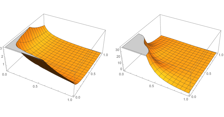
Figure 1: Graphs of $P_{s}(\mbox{\boldmath$\rho$}^{p})$ for $p=1$ (left) and $p=3$ (right)

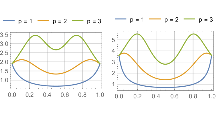
Figure 2: Graphs of $P_{s}(\mbox{\boldmath$\rho$}^{p})$ on the boundary $\rho_{1}+\rho_{2}=1$.

Fig. 2 shows clearly that $P_{c}(\mbox{\boldmath$\rho$})$ is strictly convex on its boundary $\rho_{1}+\rho_{2}=1$. The feasible solutions for $({\cal P}_{c})$ can be achieved only on the corners $\mbox{\boldmath$\rho$}=(1,0)$ and $\mbox{\boldmath$\rho$}=(0,1)$, both of them are global maximizers. Therefore, the problem $({\cal P}_{s})$ is considered to be NP-hard by traditional theories. For the SIMP problem $({\cal P}_{simp})$ with $p=2$, its global minimizer is $\mbox{\boldmath$\rho$}=(0.5,0.5)$, which is not a solution to the topology optimization problem. Although for $p=3$ the global min of $P_{s}(\mbox{\boldmath$\rho$}^{p})$ can be achieved at either $\mbox{\boldmath$\rho$}=(1,0)$ or $\mbox{\boldmath$\rho$}=(0,1)$ (see Fig. 2 (a)), these two solutions can’t be obtained by any Newton-type method since they are not a critical points. Moreover, if the constant $a=(2-\sqrt{2})/4$, the global min of $P_{s}(\mbox{\boldmath$\rho$}^{3})$ is again $\mbox{\boldmath$\rho$}=(0.5,0.5)$ (see Fig. 2(b)). This shows that $p=3$ in the SIMP method is a “magic number” only for certain materials/structures. By the fact that $P_{s}(\mbox{\boldmath$\rho$}^{p})$ is nonconvex for any given $p>1$, the SIMP problem $({\cal P}_{simp})$ is a typical “NP-hard” box constrained nonconvex minimization subjected to the knapsack condition, which can’t be solved deterministically by all traditional methods in polynomial time.

3 Canonical Dual Solution to Knapsack Problem

The canonical duality theory for solving constrained quadratic 0-1 integer programming problems was first proposed by Gao in 2007 [20]. Applications have been given to general problems in operations research [21] and recently to topology optimization for general materials [24]. In this paper, we focus mainly on linear elastic structures.

Following the standard procedure in the canonical duality theory (see [20, 30]), the canonical measure for 0-1 integer programming problem $({\cal P}_{kp})$ can be given as

$$\mbox{\boldmath$\xi$}=\Lambda(\mbox{\boldmath$\rho$})=\{\mbox{\boldmath$\rho$}\circ\mbox{\boldmath$\rho$}-\mbox{\boldmath$\rho$},\;\;\mbox{\boldmath$\rho$}^{T}\mathbf{v}-V_{c}\}:\;\;\mathbb{R}^{n}\rightarrow{\cal E}=\mathbb{R}^{n+1}.$$ (24)

where $\mbox{\boldmath$\rho$}\circ\mbox{\boldmath$\rho$}=\{\rho_{e}\rho_{e}\}\in\mathbb{R}^{n}$ represents the Hadamard product. Let

$${\cal E}_{a}:=\{\mbox{\boldmath$\xi$}=\{\mbox{\boldmath$\epsilon$},\nu\}\in\mathbb{R}^{n+1}|\;\;\mbox{\boldmath$\epsilon$}\leq 0,\;\;\nu\leq 0\}$$ (25)

be a convex cone in $\mathbb{R}^{n+1}$. Its indicator $\Psi(\mbox{\boldmath$\xi$})$ is defined by

$$\Psi(\mbox{\boldmath$\xi$})=\left\{\begin{array}[]{ll}0&\mbox{ if }\mbox{\boldmath$\xi$}\in{\cal E}_{a}\\ +\infty&\mbox{ otherwise}\end{array}\right.$$ (26)

which is a convex and lower semi-continuous (l.s.c) function in $\mathbb{R}^{n+1}$. By this function, the knapsack problem $({\cal P}_{kp})$ can be relaxed in the following unconstrained minimization form:

$$\min\left\{\Pi_{u}(\mbox{\boldmath$\rho$})=\Psi(\Lambda(\mbox{\boldmath$\rho$}))-{\bf w}^{T}\mbox{\boldmath$\rho$}\;\;|\;\;\mbox{\boldmath$\rho$}\in\mathbb{R}^{n}\right\}.$$ (27)

By the convexity of $\Psi(\mbox{\boldmath$\xi$})$, its conjugate function can be defined uniquely via the Fenchel transformation:

$$\Psi^{*}(\mbox{\boldmath$\varsigma$})=\sup_{\mbox{\boldmath$\xi$}\in\mathbb{R}^{n+1}}\{\mbox{\boldmath$\xi$}^{T}\mbox{\boldmath$\varsigma$}-\Psi(\mbox{\boldmath$\xi$})\}=\left\{\begin{array}[]{ll}0&\mbox{ if }\mbox{\boldmath$\varsigma$}\in{\cal E}_{a}^{*}\\ +\infty&\mbox{ otherwise},\end{array}\right.$$ (28)

where

$${\cal E}_{a}^{*}=\{\mbox{\boldmath$\varsigma$}=\{\mbox{\boldmath$\sigma$},\tau\}\in\mathbb{R}^{n+1}|\;\;\mbox{\boldmath$\sigma$}\geq 0,\;\;\tau\geq 0\}$$ (29)

is the dual space of ${\cal E}_{a}$.

Thus, by using the Fenchel-Young equality

$$\Psi(\mbox{\boldmath$\xi$})+\Psi^{*}(\mbox{\boldmath$\varsigma$})=\mbox{\boldmath$\xi$}^{T}\mbox{\boldmath$\varsigma$},$$ (30)

the function $\Psi(\mbox{\boldmath$\rho$})$ in (27) can be written as the Gao-Strang total complementary function [33],

$$\Xi(\mbox{\boldmath$\rho$},\mbox{\boldmath$\varsigma$})=\Lambda(\mbox{\boldmath$\rho$})^{T}\mbox{\boldmath$\varsigma$}-{\bf w}^{T}\mbox{\boldmath$\rho$}-\Psi^{*}(\mbox{\boldmath$\varsigma$}).$$ (31)

Based on this function, the canonical dual of $\Pi_{u}(\mbox{\boldmath$\rho$})$ can be defined by

$$\Pi_{u}^{d}(\mbox{\boldmath$\varsigma$})=\mbox{sta }\{\Xi(\mbox{\boldmath$\rho$},\mbox{\boldmath$\varsigma$})|\;\;\mbox{\boldmath$\rho$}\in\mathbb{R}^{n}\}=P^{d}_{u}(\mbox{\boldmath$\varsigma$})-\Psi^{*}(\mbox{\boldmath$\varsigma$}),$$ (32)

where

$$P^{d}_{u}(\mbox{\boldmath$\varsigma$})=\mbox{sta }\{\Lambda(\mbox{\boldmath$\rho$})^{T}\mbox{\boldmath$\varsigma$}-{\bf w}^{T}\mbox{\boldmath$\rho$}|\;\;\mbox{\boldmath$\rho$}\in\mathbb{R}^{n}\}=-\frac{1}{4}\mbox{\boldmath$\psi$}^{T}_{u}(\mbox{\boldmath$\varsigma$})\mathbf{G}^{-1}(\mbox{\boldmath$\varsigma$})\mbox{\boldmath$\psi$}_{u}(\mbox{\boldmath$\varsigma$})-\tau V_{c},$$ (33)

in which,

$$\mathbf{G}(\mbox{\boldmath$\varsigma$})=\ \mbox{Diag}\{\mbox{\boldmath$\sigma$}\},\;\;\;\mbox{\boldmath$\psi$}_{u}(\mbox{\boldmath$\varsigma$})=\mbox{\boldmath$\sigma$}-\tau\mathbf{v}+{\bf w}.$$

Clearly, $P_{u}^{d}(\mbox{\boldmath$\varsigma$})$ is well-defined if $\mbox{\boldmath$\sigma$}\neq{\bf 0}\in\mathbb{R}^{n}$. By the standard complementary-dual principle in the canonical duality theory, we have the main result:

Theorem 1 (Complementary-Dual Principle)

For any given $\mathbf{u}\in{\cal U}_{a}$, if $(\bar{\mbox{\boldmath$\rho$}},\bar{\mbox{\boldmath$\varsigma$}})$ is a KKT point of $\Xi$, then $\bar{\mbox{\boldmath$\rho$}}$ is a KKT point of $\Pi_{u}$, $\bar{\mbox{\boldmath$\varsigma$}}$ is a KKT point of $\Pi_{u}^{d}$, and

$$\Pi_{u}(\bar{\mbox{\boldmath$\rho$}})=\Xi(\bar{\mbox{\boldmath$\rho$}},\bar{\mbox{\boldmath$\varsigma$}})=\Pi_{u}^{d}(\bar{\mbox{\boldmath$\varsigma$}}).$$ (34)

Proof: By the convexity of $\Psi(\mbox{\boldmath$\xi$})$, we have the following canonical duality relations [17, 18]:

$$\mbox{\boldmath$\varsigma$}\in\partial\Psi(\mbox{\boldmath$\xi$})\;\;\Leftrightarrow\;\;\mbox{\boldmath$\xi$}\in\partial\Psi^{*}(\mbox{\boldmath$\varsigma$})\;\;\Leftrightarrow\;\;\Psi(\mbox{\boldmath$\xi$})+\Psi^{*}(\mbox{\boldmath$\varsigma$})=\mbox{\boldmath$\xi$}^{T}\mbox{\boldmath$\varsigma$},$$ (35)

where

$$\partial\Psi(\mbox{\boldmath$\xi$})=\left\{\begin{array}[]{ll}\mbox{\boldmath$\varsigma$}&\mbox{ if }\mbox{\boldmath$\varsigma$}\in{\cal E}_{a}^{*}\\ \emptyset&\mbox{ otherwise}\end{array}\right.$$

is the sub-differential of $\Psi$. Thus, in terms of $\mbox{\boldmath$\xi$}=\Lambda(\mbox{\boldmath$\rho$})$ and $\mbox{\boldmath$\varsigma$}=\{\mbox{\boldmath$\sigma$},\tau\}$, the canonical duality relations (35) can be equivalently written as

$$\mbox{\boldmath$\rho$}\circ\mbox{\boldmath$\rho$}-\mbox{\boldmath$\rho$}\leq 0\;\;\Leftrightarrow\;\;\mbox{\boldmath$\sigma$}\geq 0\;\;\Leftrightarrow\;\;\mbox{\boldmath$\sigma$}^{T}(\mbox{\boldmath$\rho$}\circ\mbox{\boldmath$\rho$}-\mbox{\boldmath$\rho$})=0\;\;$$ (36)

$$\mbox{\boldmath$\rho$}^{T}\mathbf{v}-V_{c}\leq 0\;\;\Leftrightarrow\;\;\tau\geq 0\;\;\Leftrightarrow\;\;\tau(\mbox{\boldmath$\rho$}^{T}\mathbf{v}-V_{c})=0.$$ (37)

These are exactly the KKT conditions for the inequality constraints $\mbox{\boldmath$\rho$}\circ\mbox{\boldmath$\rho$}-\mbox{\boldmath$\rho$}\leq 0$ and $\mbox{\boldmath$\rho$}^{T}\mathbf{v}-V_{c}\leq 0$. Thus, $(\bar{\mbox{\boldmath$\rho$}},\bar{\mbox{\boldmath$\varsigma$}})$ is a KKT point of $\Xi$ if and only if $\bar{\mbox{\boldmath$\rho$}}$ is a KKT point of $\Pi_{u}$, $\bar{\mbox{\boldmath$\varsigma$}}$ is a KKT point of $\Pi_{u}^{d}$. The equality (34) holds due to the canonical duality relations in (35). ∎

By the complementarity condition $\mbox{\boldmath$\sigma$}^{T}(\mbox{\boldmath$\rho$}\circ\mbox{\boldmath$\rho$}-\mbox{\boldmath$\rho$})=0$ in (36), we know that $\mbox{\boldmath$\rho$}\circ\mbox{\boldmath$\rho$}=\mbox{\boldmath$\rho$}$ if $\mbox{\boldmath$\sigma$}>0$. Let

$${\cal S}_{a}^{+}=\{\mbox{\boldmath$\varsigma$}=\{\mbox{\boldmath$\sigma$},\tau\}\in{\cal E}_{a}^{*}|\;\;\mbox{\boldmath$\sigma$}>0\}.$$ (38)

Then for any given $\mbox{\boldmath$\varsigma$}=\{\mbox{\boldmath$\sigma$},\tau\}\in{\cal S}^{+}_{a}$, the function $\Xi(\cdot,\mbox{\boldmath$\varsigma$}):\mathbb{R}^{n}\rightarrow\mathbb{R}$ is convex and the canonical dual function of $P_{u}$ in $({\cal P}_{kp})$ can be well-defined by

$$P^{d}_{u}(\mbox{\boldmath$\varsigma$})=\min_{\mbox{\boldmath$\rho$}\in\mathbb{R}^{n}}\Xi(\mbox{\boldmath$\rho$},\mbox{\boldmath$\varsigma$})=-\sum_{e=1}^{n}\frac{1}{4}(\sigma_{e}+w_{e}-\tau v_{e})^{2}\sigma_{e}^{-1}-\tau V_{c}.$$ (39)

Thus, the canonical dual problem of $({\cal P}_{kp})$ can be proposed as the following:

$$({\cal P}^{d}_{u}):\;\;\;\max\{P^{d}_{u}(\mbox{\boldmath$\sigma$},\tau)|\;\;(\mbox{\boldmath$\sigma$},\tau)\in{\cal S}^{+}_{a}\}.$$ (40)

This is a concave maximization problem over a convex subset in continuous space, which can be solved via well-developed convex optimization methods to obtain global optimal solution. Thus, whence a canonical dual solution $\bar{\mbox{\boldmath$\varsigma$}}$ is obtained, the solution $\bar{\mbox{\boldmath$\rho$}}$ to the primal problem can be defined in an analytical form of $\bar{\mbox{\boldmath$\varsigma$}}$.

Theorem 2 (Analytical Solution)

For any given $\mathbf{u}\in{\cal U}_{a}$ such that ${\bf w}=\mathbf{c}(\mathbf{u})\in\mathbb{R}^{n}_{+}$, if $\bar{\mbox{\boldmath$\varsigma$}}=(\bar{\mbox{\boldmath$\sigma$}},\bar{\tau})\in{\cal S}^{+}_{a}$ is a solution to $({\cal P}^{d}_{u})$, then

$$\bar{\mbox{\boldmath$\rho$}}=\frac{1}{2}[\mbox{Diag}(\bar{\mbox{\boldmath$\sigma$}})]^{-1}(\bar{\mbox{\boldmath$\sigma$}}-\bar{\tau}\mathbf{v}+{\bf w})$$ (41)

is a unique global optimal solution to $({\cal P}_{kp})$ and

$$P_{u}(\bar{\mbox{\boldmath$\rho$}})=\min_{\mbox{\boldmath$\rho$}\in{\cal Z}_{a}}P_{u}(\mbox{\boldmath$\rho$})=\max_{\mbox{\boldmath$\varsigma$}\in{\cal S}^{+}_{a}}P^{d}_{u}(\mbox{\boldmath$\varsigma$})=P^{d}_{u}(\bar{\mbox{\boldmath$\varsigma$}}).$$ (42)

Proof: It is easy to prove that for any given $\mathbf{u}\in{\cal U}_{a}$, the canonical dual function $P^{d}_{u}(\mbox{\boldmath$\varsigma$})$ is concave on the open convex set ${\cal S}^{+}_{a}$. If $\bar{\mbox{\boldmath$\varsigma$}}$ is a KKT point of $P^{d}_{u}(\mbox{\boldmath$\varsigma$})$, then it must be a unique global maximizer of $P^{d}_{u}(\mbox{\boldmath$\varsigma$})$ on ${\cal S}^{+}_{a}$. By Theorem 1 we know that if $\bar{\mbox{\boldmath$\varsigma$}}=\{\bar{\mbox{\boldmath$\sigma$}},\bar{\tau}\}\in{\cal S}^{+}_{a}$ is a KKT point of $\Pi_{u}^{d}(\mbox{\boldmath$\varsigma$})$, then $\bar{\mbox{\boldmath$\rho$}}=\mbox{\boldmath$\rho$}(\bar{\mbox{\boldmath$\varsigma$}})$ defined by (41) must be a KKT point of $\Pi_{u}(\mbox{\boldmath$\rho$})$ (see [20, 24]). Since $\Xi(\mbox{\boldmath$\rho$},\mbox{\boldmath$\varsigma$})$ is a saddle function on $\mathbb{R}^{n}\times{\cal S}^{+}_{a}$, we have

$$\min_{\mbox{\boldmath$\rho$}\in{\cal Z}_{a}}P_{u}(\mbox{\boldmath$\rho$}) = \min_{\mbox{\boldmath$\rho$}\in\mathbb{R}^{n}}\Pi_{u}(\mbox{\boldmath$\rho$})=\min_{\mbox{\boldmath$\rho$}\in\mathbb{R}^{n}}\max_{\mbox{\boldmath$\varsigma$}\in{\cal S}^{+}_{a}}\Xi(\mbox{\boldmath$\rho$},\mbox{\boldmath$\varsigma$})=\max_{\mbox{\boldmath$\varsigma$}\in{\cal S}^{+}_{a}}\min_{\mbox{\boldmath$\rho$}\in\mathbb{R}^{n}}\Xi(\mbox{\boldmath$\rho$},\mbox{\boldmath$\varsigma$})$$

$$= \max_{\mbox{\boldmath$\varsigma$}\in{\cal S}^{+}_{a}}\Pi_{u}^{d}(\mbox{\boldmath$\varsigma$})=\max_{\mbox{\boldmath$\varsigma$}\in{\cal S}^{+}_{a}}P^{d}_{u}(\mbox{\boldmath$\varsigma$}).$$

Since $\bar{\mbox{\boldmath$\sigma$}}>0$, the complementarity condition in (36) leads to

$$\bar{\mbox{\boldmath$\rho$}}\circ\bar{\mbox{\boldmath$\rho$}}-\bar{\mbox{\boldmath$\rho$}}=0\;\;\mbox{ i.e. }\bar{\mbox{\boldmath$\rho$}}\in\{0,1\}^{n}.$$

Thus, we have

$$P_{u}(\bar{\mbox{\boldmath$\rho$}})=\min_{\mbox{\boldmath$\rho$}\in{\cal Z}_{a}}P_{u}(\mbox{\boldmath$\rho$})=\max_{\mbox{\boldmath$\varsigma$}\in{\cal S}^{+}_{a}}P^{d}_{u}(\mbox{\boldmath$\varsigma$})=P^{d}_{u}(\bar{\mbox{\boldmath$\varsigma$}})$$

as required. ∎

Theorem 2 shows that although the canonical dual problem is a concave maximization in continuous space, it produces the analytical solution (41) to the well-known integer Knapsack problem $({\cal P}_{kp})$! This analytical solution was first proposed by Gao in 2007 for general quadratic integer programming problems (see Theorem 3, [20]). The indicator function of a convex set in (26) and its sub-differential were first introduced by J.J. Moreau in 1963 in his study on unilateral constrained problems in contact mechanics [50]. His pioneering work laid a foundation for modern analysis and the canonical duality theory. In solid mechanics, the indicator of a plastic yield condition is also called a super-potential. Its sub-differential leads to a general constitutive law and a unified pan-penalty finite element method in plastic limit analysis [13]. In mathematical programming, the canonical duality leads to a unified framework for nonlinear constrained optimization problems in multi-scale systems [32, 44].

4 Canonical Penalty-Duality Method and Algorithm

According to Theorem 2, the global optimal solution to $({\cal P}_{kp})$ can be obtained by solving its canonical dual problem $({\cal P}_{kp}^{d})$. However, the rate of convergence could be very slow since $P^{d}_{u}(\mbox{\boldmath$\sigma$},\tau)$ is nearly a linear function of $\mbox{\boldmath$\sigma$}\in\mathbb{R}^{n}_{+}$ when $\sigma$ is far from its origin. In order to overcome this problem, a so-called $\beta$-perturbed canonical dual method was proposed by Gao and Ruan in integer programming [30]. This $\beta$-perturbation is actually based on a so-called canonical penalty-duality method, i.e. the integer constraint in $({\cal P}_{kp})$ is first written in the canonical form $\mbox{\boldmath$\epsilon$}=\mbox{\boldmath$\rho$}\circ\mbox{\boldmath$\rho$}-\mbox{\boldmath$\rho$}={\bf 0}$, then is relaxed by the external penalty method, while the volume constraint is simply relaxed by the Lagrange multiplier $\tau\geq 0$, thus, the knapsack problem can be reformulated as the following canonical penalty-duality form

$$\min_{\mbox{\boldmath$\rho$}\in\mathbb{R}^{n}}\max_{\tau\geq 0}\left\{P_{\beta}(\mbox{\boldmath$\rho$},\tau)=\beta\|\mbox{\boldmath$\rho$}\circ\mbox{\boldmath$\rho$}-\mbox{\boldmath$\rho$}\|^{2}-{\bf w}^{T}\mbox{\boldmath$\rho$}+\tau(\mathbf{v}^{T}\mbox{\boldmath$\rho$}-V_{c})\right\},$$ (43)

where $\beta>0$ is a penalty parameter. As we can see clearly that due to the nonlinearity of the canonical constraint $\mbox{\boldmath$\epsilon$}(\mbox{\boldmath$\rho$})=0$, the canonical penalty function is nonconvex in $\rho$. This is the reason why the standard penalty method can’t be used for solving general nonlinearly constrained problems. However, by using the canonical duality theory, this nonconvex min-max problem can be equivalently reformulated as a canonical dual problem:

$$({\cal P}^{d}_{\beta}):\;\;\max\left\{P^{d}_{\beta}(\mbox{\boldmath$\sigma$},\tau)=P^{d}_{u}(\mbox{\boldmath$\sigma$},\tau)-\frac{1}{4}\beta^{-1}\mbox{\boldmath$\sigma$}^{T}\mbox{\boldmath$\sigma$}|\;\;\{\mbox{\boldmath$\sigma$},\tau\}\in{\cal S}^{+}_{a}\;\right\},$$ (44)

which is exactly the same canonical penalty-duality problem proposed by Gao for solving the knapsack problem in topology optimization [24].

Theorem 3 (Perturbed Solution to Knapsack Problem)

For any given $\mathbf{u}\in{\cal U}_{a}$, $V_{c}>0$, and $\beta>0$ such that ${\bf w}=\mathbf{c}(\mathbf{u})\in\mathbb{R}^{n}_{+}$, the problem $({\cal P}^{d}_{\beta}))$ has at most one solution $\mbox{\boldmath$\varsigma$}_{\beta}=(\mbox{\boldmath$\sigma$}_{\beta},\tau_{\beta})\in{\cal S}^{+}_{a}$. Moreover, there exists a $\beta_{c}\gg 0$ such that for any given $\beta\in[\beta_{c},+\infty)$, the vector

$$\mbox{\boldmath$\rho$}_{\beta}=\frac{1}{2}[\mbox{Diag}(\mbox{\boldmath$\sigma$}_{\beta})]^{-1}(\mbox{\boldmath$\sigma$}_{\beta}-\tau_{\beta}\mathbf{v}+{\bf w})\in\{0,1\}^{n}$$ (45)

is a global optimal solution to $({\cal P}_{kp})$.

Proof. It is easy to show that for any given $\beta>0$,

$$P^{d}_{\beta}(\mbox{\boldmath$\sigma$},\tau)=-\frac{1}{4}\left[\sum_{e=1}^{n}(\sigma_{e}+w_{e}-\tau v_{e})^{2}\sigma_{e}^{-1}+\beta^{-1}\sigma^{2}_{e}\right]-\tau V_{c}$$ (46)

is strictly concave on the open convex set ${\cal S}^{+}_{a}$. Thus, $({\cal P}^{d}_{\beta})$ has a unique solution if $w_{e}-\tau v_{e}\neq 0\;\;\forall e=1,\dots,n$. Indeed, the criticality condition $\nabla P^{d}_{\beta}(\mbox{\boldmath$\varsigma$})=0$ leads to the following canonical dual algebraic equations:

$$2\beta^{-1}\sigma_{e}^{3}+\sigma_{e}^{2}=(\tau v_{e}-w_{e})^{2},\;\;e=1,\dots,n,$$ (47)

$$\sum_{e=1}^{n}\frac{1}{2}\frac{v_{e}}{\sigma_{e}}(\sigma_{e}-v_{e}\tau+w_{e})-V_{c}=0.$$ (48)

It was proved by the author (see Section 3.4.3, [18] and the Appendix of this paper) that for any given $\beta>0$ and $\theta_{e}(\tau)=\tau v_{e}-w_{e}\neq 0,\ e=1,\dots,n$, the canonical dual algebraic equation (47) has a unique positive real solution

$$\sigma_{e}=\frac{1}{6}\beta[-1+\phi_{e}(\tau)+\phi_{e}^{c}(\tau)]>0,\;\;e=1,\dots,n$$ (49)

where

$$\phi_{e}(\tau)=\eta^{-1/3}\left[2\theta_{e}(\tau)^{2}-\eta+2i\sqrt{\theta_{e}(\tau)^{2}(\eta-\theta_{e}(\tau)^{2})}\right]^{1/3},\;\;\eta=\frac{\beta^{2}}{27},$$

and $\phi_{e}^{c}$ is the complex conjugate of $\phi_{e}$, i.e. $\phi_{e}\phi_{e}^{c}=1$. Also, the canonical dual algebraic equation (48) has a unique solution

$$\tau=\frac{\sum_{e=1}^{n}v_{e}(1+w_{e}/\sigma_{e})-2V_{c}}{\sum_{e=1}^{n}v_{e}^{2}/\sigma_{e}}.$$ (50)

This shows that the perturbed canonical dual problem $({\cal P}^{d}_{\beta})$ has a unique solution $\mbox{\boldmath$\varsigma$}_{\beta}$ in ${\cal S}^{+}_{a}$ if $\theta_{e}(\tau)=\tau v_{e}-w_{e}\neq 0,\ e=1,\dots,n$. Thus, the density distribution $\mbox{\boldmath$\rho$}_{\beta}$ can be analytically obtained by substituting (49) and (50) into (45). By the fact that $\lim_{\beta\rightarrow\infty}\Pi^{d}_{\beta}(\mbox{\boldmath$\varsigma$})=\Pi^{d}_{u}(\mbox{\boldmath$\varsigma$})$, there must exists a $\beta_{c}>0$ such that

$$\mbox{\boldmath$\rho$}_{\beta}\in\{0,1\}^{n}\;\;\forall\beta\geq\beta_{c}.$$ (51)

By Theorem 2 we know that this perturbed solution must be a global minimum solution to the knapsack problem. A similar proof of this theorem was given in [30]. $\Box$

By Theorems 2 and 3 we know that for a given desired volume $V_{c}>0$, the optimal density distribution can be analytically obtained in terms of its canonical dual solution in continuous space. By the fact that $({\cal P}_{bk})$ is a bilevel mixed integer nonlinear programming, numerical optimization depends sensitively on the initial volume $V_{0}$. If $\mu_{c}=V_{c}/V_{0}\ll 1,$ any given iteration method could lead to unreasonable numerical solutions. In order to resolve this problem, a volume reduction control parameter $\mu\in(\mu_{c},1)$ was introduced in [24] to produce a volume sequence $V_{\gamma}=\mu V_{\gamma-1}$ ($\gamma=1,\dots,\gamma_{c}$) such that $V_{\gamma_{c}}=V_{c}$ and for any given $V_{\gamma}\in[V_{c},V_{0}]$, the problem $({\cal P}_{bl})$ is replaced by

$$({\cal P}_{bk})^{\gamma}:\;\; \min\{\mathbf{f}^{T}\bar{\mathbf{u}}-\mathbf{c}(\bar{\mathbf{u}})^{T}\mbox{\boldmath$\rho$}^{p}|\;\;\mathbf{v}^{T}\mbox{\boldmath$\rho$}\leq V_{\gamma},\;\;\mbox{\boldmath$\rho$}\in\{0,1\}^{n}\}$$ (53)

$$\mbox{s.t.}\;\;\bar{\mathbf{u}}(\mbox{\boldmath$\rho$})=\arg\min\{\Pi_{h}(\mathbf{u},\mbox{\boldmath$\rho$})|\;\;{\mathbf{u}\in{\cal U}_{a}}\}.$$

The initial values for solving this $\gamma$-th problem are $V_{\gamma-1},\mathbf{u}_{\gamma-1},$ $\mbox{\boldmath$\rho$}_{\gamma-1}$. Based on the above strategies, the canonical duality algorithm (i.e. CDT [24]) for solving the general topology optimization problem $({\cal P}_{bk})$ can be proposed in Algorithm 1.

Algorithm 1 Canonical Dual Algorithm for Topology Optimization (CDT)

1:Input parameters: $\mu$, $\beta$ and error allowances: $\omega_{1},\omega_{2}>0$.

2:Initiate $\mbox{\boldmath$\rho$}^{0}=\{1\}\in\mathbb{R}^{n}$, $V_{0},\tau^{0}>0$, and let $\gamma=1$.

3:Solve the lower-level optimization problem (9):

$$\mathbf{u}^{\gamma}=\arg\min\{\Pi_{h}(\mathbf{u},\mbox{\boldmath$\rho$}^{\gamma-1})|\;\;\mathbf{u}\in{\cal U}_{a}\}.$$

4:Compute ${\bf w}^{\gamma}=\{w_{e}^{\gamma}\}=\mathbf{c}(\mathbf{u}^{\gamma})$ via (5), $V_{\gamma}=\max\{V_{c},\mu V_{\gamma-1}\}$. Let $k=1$.

5:Compute the canonical dual solutions $\mbox{\boldmath$\sigma$}^{k}=\{\sigma_{e}^{k}\}$ and $\tau^{k}$ by

$$\sigma_{e}^{k}=\frac{1}{12}\beta[-1+\phi(\tau^{k-1})+\phi^{c}(\tau^{k-1})],\;\;e=1,\dots,n.$$

$$\tau^{k}=\frac{\sum_{e=1}^{n}v_{e}(1+w^{\gamma}_{e}/\sigma_{e}^{k})-2V_{\gamma}}{\sum_{e=1}^{n}v_{e}^{2}/\sigma_{e}^{k}}.$$

6:If $|P^{d}_{u}(\mbox{\boldmath$\sigma$}^{k},\tau^{k})-P^{d}_{u}(\mbox{\boldmath$\sigma$}^{k-1},\tau^{k-1})|>\omega_{1}$ , then let $k=k+1$, go to Step 5; Otherwise, continue.

7:Compute the upper-level solution $\mbox{\boldmath$\rho$}^{\gamma}$ by

$$\rho^{\gamma}_{e}=\frac{1}{2}[1-(\tau^{k}v_{e}-w^{\gamma}_{e})/\sigma_{e}^{k}],\;\;e=1,\dots,n.$$

8:If $|P_{u}(\mbox{\boldmath$\rho$}^{\gamma})-P_{u}(\mbox{\boldmath$\rho$}^{\gamma-1})|\leq\omega_{2}$ and $V_{\gamma}\leq V_{c}$ , then stop; Otherwise, continue.

9:Let $\tau^{0}=\tau^{k}$, and $\gamma=\gamma+1$. Go to Step 3.

Remark 2 (Volume Reduction and Computational Complexity)

 
Theoretically speaking, for any given sequence $\{V_{\gamma}\}$ we should have

$$({\cal P}_{bk})=\lim_{\gamma\rightarrow\gamma_{c}}({\cal P}_{bk})^{\gamma}.$$ (54)

In reality, different sequence $\{V_{\gamma}\}$ may produce totally different structural topology. This is an intrinsic difficulty for all bi-level optimal design problems. By the facts that there are only two loops in the CDT algorithm, i.e. the $\gamma$-loop and the $k$-loop, and the canonical dual solution is analytically given in the $k$-loop, the main computing is the $m\times m$ matrix inversion in the $\gamma$-loop. The complexity for the Gauss-Jordan elimination is $O(m^{3})$. Therefore, the CDT is a polynomial-time algorithm.

The optimization problem of BESO as formulated in [36] is posed in the form of minimization of mean compliance, i.e. the problem $({\cal P}_{c})$. Since the alternative iteration is adopted by BESO, which leads to an anti-Knapsack problem by (19) , therefore, the BESO should theoretically produce only trivial solution at each volume evolution. However, instead of solving the anti-Knapsack problem (19), a comparison method is used to keep those elements which store more strain energy. So, the BESO is actually a direct method for solving the knapsack problem $({\cal P}_{kp})$. This is the reason why the numerical results obtained by BESO are similar to that by CDT (see Section 6). But, the direct method is not a polynomial-time algorithm. Due to the combinatorial complexity, this popular method is computationally expensive and can be used only for small sized problems. This is the very reason why the knapsack problem has been considered as NP-complete for all existing direct approaches. $\clubsuit$

5 Symmetry and NP-Hardness for Knapsack Problem

There is a hidden condition in the proof of Theorem 3, which is actually the limitation of the canonical duality theory.

Theorem 4 (Existence of Solution to Knapsack Problem)

For any given $\mathbf{v},{\bf w}\in\mathbb{R}^{n}_{+}$, if there exists a constant $\tau_{c}>0$ such that

$$\theta_{e}(\tau_{c})=\tau_{c}v_{e}-w_{e}\neq{0}\;\;\forall e=1,\dots,n$$ (55)

the canonical dual feasible set ${\cal S}^{+}_{a}\neq\emptyset$ and the knapsack problem $({\cal P}_{kp})$ has a unique solution. Otherwise, if $\theta_{e}(\tau_{c})=0$ for at least one $e\in\{1,\dots,n\}$, then ${\cal S}^{+}_{a}=\emptyset$ and $({\cal P}_{kp})$ has at least two solutions.

Proof. From the proof of Theorem 3 we know that for any given $\beta>0$, if thre exists a $\tau_{c}>0$ such that the conditions in (55) hold, the canonical dual algebraic equation (47) has a unique $\sigma_{e}>0$ for every $e=1,\dots,n$, which can be obtained analytically by (49) see Theorem 3.4.4 in [18]). Therefore, the canonical dual problem $({\cal P}^{d}_{kp})$ has a unique solution in ${\cal S}^{+}_{a}$. Correspondingly, the primal problem $({\cal P}_{kp})$ has a unique solution defined by either (41) or (45). If $\theta_{e}(\tau_{c})=0$ for at least one $e=1,\dots,n$, the equation $2\beta^{-1}\sigma_{e}^{3}+\sigma_{e}^{2}=0$ has two solutions $\sigma_{e}=0$. In this case, the KKT points of $({\cal P}^{d}_{\beta})$ are located on the boundary of the open set ${\cal S}^{+}_{a}$. Therefore, ${\cal S}^{+}_{a}=\emptyset$ and $({\cal P}_{kp})$ has at least two solutions. $\Box$

Remark 3 (NP-Hard Conjecture, Symmetry, and Linear Perturbation)

Theorem 4 shows that under the condition (55), the well-known knapsack problem is not NP-hard and can be solved analytically by the canonical duality theory. It is discovered recently [25] that the critical value $\tau_{c}$ in (55) can be deterministically given by

$$\tau_{c}=\arg\min_{\tau\geq 0}\left\{\sum_{e=1}^{n}(|w_{e}-\tau v_{e}|-\tau v_{e})+2\tau V_{c}\right\}.$$ (56)

Otherwise, as long as $\theta_{e}(\tau_{c})=0$ for at least one $e=1,\dots,n$, the solution to $({\cal P}_{kp})$ can’t be written in the analytical form (45), and the knapsack problem could be really NP-hard. Actually, it is a conjecture first proposed by the author in 2007 [20], i.e.

Conjecture of NP-Hardness: A global optimization problem is NP-hard if its canonical dual problem has no solution in ${\cal S}^{+}_{a}$.

It is also an open problem left in [21, 30]. The reason for NP-hard problems and possible solutions were discussed recently in [23].

Geometrically speaking, the reason for multiple solutions of $({\cal P}_{kp})$ is due to certain symmetry on the modeling, boundary condition and the external load. By the fact that nothing is perfect in this real world, a perfect symmetry is not allowed for any real-world problem. Mathematically speaking, if a problem has multiple solutions, this problem is not well-posed [22]. In order to solve such NP-hard problems, the key idea is to break the symmetry. A linear perturbation method has been proposed by the author and his co-workers with successful applications in hard cases of trust region method [9], nonconvex constrained optimization [51], and integer programming [67]. $\clubsuit$

The symmetry plays a fundamental rule in mathematical modeling. But, it is also a main reason that leads to chaos in nonlinear dynamics, post-buckling in large deformation mechanics, NP-hard problems in complex systems [27, 45], and the well-known paradox of Buridan’s ass.

Example 1 (Buridan’s Ass)

A donkey facing two identical hay piles starves to death because reason provides no grounds for choosing to eat one rather than the other. Mathematically, this is a knapsack problem:

$$\max\{w_{1}\rho_{1}+w_{2}\rho_{2}|\;\;\;w_{1}=w_{2}=w,\;\;\rho_{1}+\rho_{2}\leq 1,\;\;(\rho_{1},\rho_{2})\in\{0,1\}^{2}\}$$ (57)

Due to the symmetries: $v_{1}=v_{2}=1,$ and $w_{1}=w_{2}=w$, the solution to (56) is $\tau_{c}=w$. Therefore, $\theta_{e}(\tau_{c})=0\;\;\forall e=1,2$ and by Theorem 4 this problem has multiple (two) solutions, which is NP-Hard to this donkey.

To solve this problem, a linear perturbation term $\epsilon\rho_{1}$ can be added to the cost function to break the symmetry. For $w=2,\;\;\epsilon=0.05$, we have $\tau_{c}=2.0184$. So the condition (55) holds for $e=1,2$ and by the canonical duality theory, the perturbed Buridan’s ass problem has a unique solution $\mbox{\boldmath$\rho$}=(1,0)$.

Example 2 (Symmetrical Truss Topology Optimization)

Let us consider a structure proposed in [60] (see Fig. 3) with six bars that are grouped into 2 groups. Each group has the same cross sectional area, which is the design variable. The group stiffness matrices and load of this structure are:

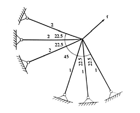
Figure 3: Symmetrical truss with symmetrical load

$$\mathbf{K}_{1}=\left[\begin{array}[]{cc}a&0\\ 0&b\end{array}\right],\;\;\mathbf{K}_{2}=\left[\begin{array}[]{cc}b&0\\ 0&a\end{array}\right],\;\;\mathbf{f}=\left[\begin{array}[]{c}1\\ 1\end{array}\right],\;\;a=\frac{2-\sqrt{2}}{2},\;\;b=\frac{4+\sqrt{2}}{2}.$$

For this linear elastic system, the associated problem $({\cal P}_{le})$ is

$$({\cal P}_{le}):\;\; \min \{\mathbf{f}^{T}\mathbf{u}-\mbox{\boldmath$\rho$}^{T}\mathbf{c}(\mathbf{u})|\;\;\;\;\rho_{1}+\rho_{2}\leq 1,\;\;\mbox{\boldmath$\rho$}\in\{0,1\}^{2}\}$$ (58)

s.t. $$(\rho_{1}\mathbf{K}_{1}+\rho_{2}\mathbf{K}_{2})\mathbf{u}=\mathbf{f},$$ (59)

where ${\bf w}=\mathbf{c}(\mathbf{u})=\frac{1}{2}(au_{1}^{2}+bu_{2}^{2},\;\;bu_{1}^{2}+au_{2}^{2})$ . Due to the symmetry, for a given $V_{0}=2$ and $\mbox{\boldmath$\rho$}_{0}=(1,1)$ we have $\mathbf{u}_{0}=(1/(a+b),1/(a+b))$, $\mathbf{c}(\mathbf{u}_{0})=(w_{1},w_{2})$ with $w_{1}=w_{2}=1/(a+b)$. Thus, the upper-level optimization (58) for the first iteration is exactly the Buridan ass problem. Clearly, this problem is artificial as it impossible to have a perfectly symmetrical truss with the perfect load $\mathbf{f}=(1,1)$. By using linear perturbation $\mathbf{f}_{\epsilon}=(1+\epsilon,1)$, for any $\epsilon>0$ we have $u_{1}>u_{2}$ and $w_{1}<w_{2}$. The CDT algorithm can produce a unique global optimal solution $\mbox{\boldmath$\rho$}^{+}=(0,1)$. Dually, for $\epsilon<0$, we have $\mbox{\boldmath$\rho$}^{-}=(1,0)$, and we have $\Pi_{h}(\mathbf{u}(\mbox{\boldmath$\rho$}^{+}),\mbox{\boldmath$\rho$}^{+})=\Pi_{h}(\mathbf{u}(\mbox{\boldmath$\rho$}^{-}),\mbox{\boldmath$\rho$}^{-})=-\frac{1}{2}(1/a+1/b)$.

6 Applications to Benchmark Problems and Novelty

The proposed CDT algorithm for topology optimization has been implemented in Matlab. The CDT code for 2-D topology optimization is based on the popular 88-line SIMP code (TOP88) proposed by Andreassen et al [2]. By the facts that the density distribution is solved analytically at each iteration and no density filter is needed, the CDT code has only 66-lines. The CDT code for 3-D topology optimization is based on the TOP3D code proposed by Liu and Tovar [42]. The CDT code has been performed for various numerical examples to test its performance. For the purpose of illustration, the applied load and geometry data are chosen as dimensionless. Young’s modulus and Poisson’s ratio of the material are taken as $E=1$ and $\nu=0.3$, respectively. The stiffness matrix of the structure in CDT algorithm is given by

$$\mathbf{K}(\mbox{\boldmath$\rho$})=\sum_{e=1}^{n}[E_{\min}+(E-E_{\min})\rho_{e}]\mathbf{K}_{e},\;\;E_{\min}=10^{-9}.$$

Clearly, we have $\mathbf{K}({\bf 1})=\sum_{e=1}^{n}E\mathbf{K}_{e}$ and $\mathbf{K}({\bf 0})=\sum_{e=1}^{n}E_{\min}\mathbf{K}_{e}$. The reason for choosing $E_{\min}\neq 0$ is to avoid singularity in computation. To compare with other approaches, the parameters penal $=3$, rmin = 1.5, and ft=1.0 are used in the SIMP 88-line code, BESO code, and the TOP3D code. The error allowances are set to be $\omega_{1}=2e-16$ for CDT algorithm and $\omega_{2}=10^{-2}$ for all methods (SIMP is usally failed to converge if $\omega$ is too small). The initial value for $\tau$ used in CDT is $\tau^{0}=1$. We take the design domain $V_{0}=1$, the initial design variable $\mbox{\boldmath$\rho$}^{0}=\{1\}^{n}$ for both CDT and BESO algorithms. All computations are performed by a HP laptop computer with Processor Intel Core I7-4810, CPU @ 2.80GHz and memory 2.80 GB.

6.1 MBB Beam Problem

The first example is the well-known benchmark Messerschmitt-Bölkow-Blohm (MBB) beam problem in topology optimization (see Fig. 4). The design domain is $L\times 2h=180\times 60$. Performance of the CDT method is first tasted for different mesh resolutions. Results in Fig. 5 show that for any given mesh resolutions, the CDT method produces precise integer solutions without using filter. Clearly, the finer the resolution, the smaller the compliance with better result (almost no checkerboard).

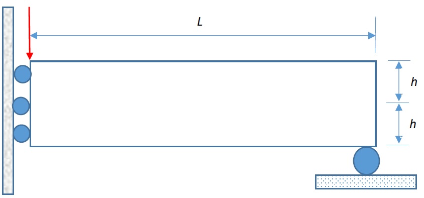
Figure 4: The design domain for a half MBB beam with external load

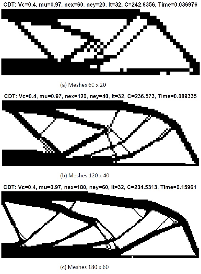
Figure 5: Optimal structures by different mesh resolutions with $\mu_{c}=0.4$ at $\mu=0.97$.

To compare with the SIMP and BESO methods, we use the same mesh resolution of $180\times 60$ but with different volume fractions. The volume reduction rate is fixed to be $\mu=0.975$ for both CDT and BESO. Computational results are reported in Figure 6, which show clearly that for any given volume fraction $\mu_{c}$, the CDT method produces better results within the significantly short times.

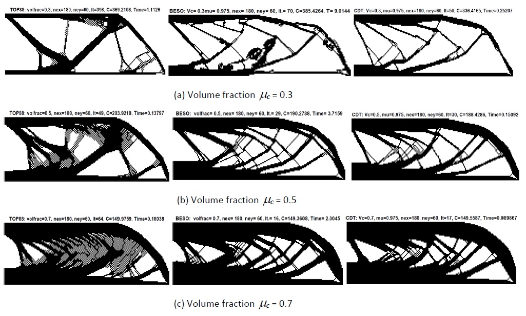
Figure 6: Computational results by SIMP (left), BESO (middle), and CDT (right) with different volume fractions $\mu_{c}=V_{c}/V_{0}$. For $\mu_{c}=0.3$, the TOP88 code failed to converge. The result reported in (a) is the out put at the iteration It = 398.

6.2 2-D Cantilever Beam Problem

The second example is the 2-D classical long cantilever beam (see Fig. 7).

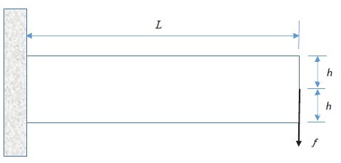
Figure 7: The design domain for a long cantilever beam with external load

For this benchmark problem, we first let the volume fraction $\mu_{c}=0.5$. Computational results obtained by the CDT and by SIMP and BESO are summarized in Fig. 8. Clearly, the precise solid-void solution produced by the CDT method is much better than that by other methods.

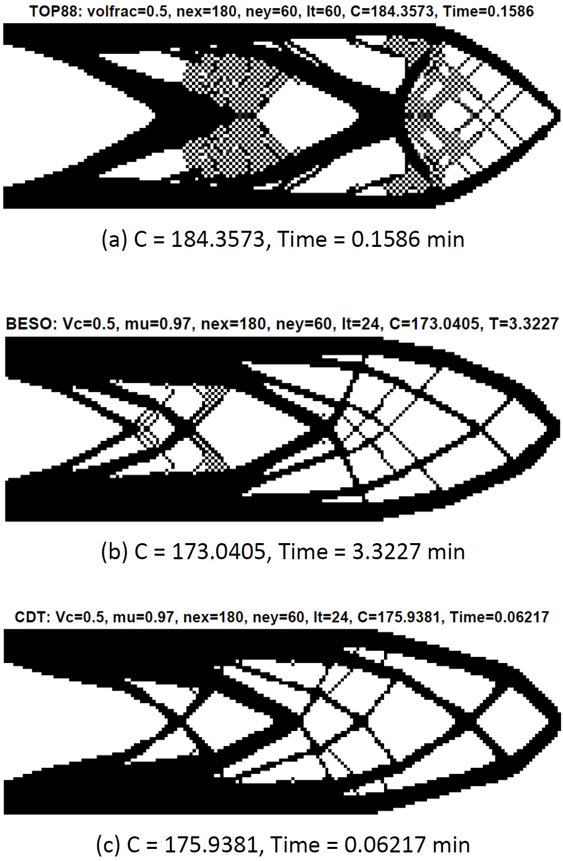
Figure 8: Computational results by SIMP (a), BESO (b) and CDT (c).

The second test for this problem is the comparison of the three methods with different volume fractions. From Fig. 9 one can see clearly that the CDT produces mechanically sound structures with the shortest computing time. A large range of checkerboards is observed in the results by SIMP, a small range of checkerboards is observed in the results by BESO, while almost no such pattern for the proposed CDT method. For $\mu_{c}=0.4$, the SIMP code does not converge and the result reported in Fig. 9(a) is the output at the 629th iteration. This test also revealed an important truth, i.e. as the volume fraction $\mu_{c}$ is decreasing, the strain energies produced by all three methods are increasing instead of decreasing. This shows clearly that the minimum strain energy problem is incorrect for topology optimization.

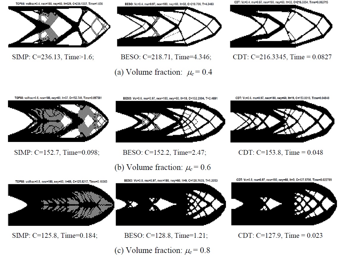
Figure 9: Comparison of computational results by SIMP (left), BESO (middle) and CDT (right) with different volume fractions.

By the fact that the BESO is a direct method for solving the correct knapsack problem, although it can produce the results similar to those by the CDT, it is not a polynomial-time algorithm. Fig. 10 verified this truth. For the given mesh resolution $180\times 60$, and $V_{c}=0.5$, $\mu=0.975$, both methods produce similar target function (i.e. strain energy $C(\mbox{\boldmath$\rho$},\mathbf{u})=\frac{1}{2}\mathbf{u}^{T}\mathbf{K}(\mbox{\boldmath$\rho$})\mathbf{u}$) (see Fig. 10(a,b)), but the BESO’s computing time is exponentially blowing up as the increase in the mesh numbers (see (see Fig. 10(c)). Results in Fig. 10(a,b) show that both BESO and CDT are maximizing the strain energy, i.e. they are solving the knapsack problem $({\cal P}_{kp})$, while the SIMP method is minimizing the strain energy, i.e. it is solving $({\cal P}_{s})$.

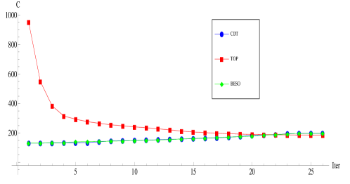
(a) Convergence test for SIMP (red), BESO (green), and CDT (blue)

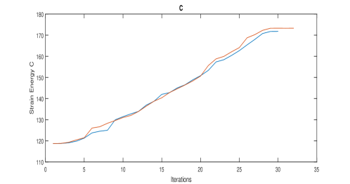
(b) Convergence test for BESO (red) and CDT (blue), $V_{c}=0.5,\;\;\mu=0.975$

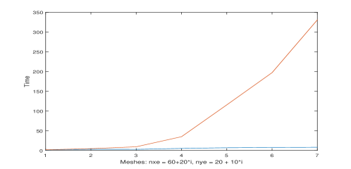
(c) Computing times by BESO (red) and CDT (blue), $V_{c}=0.5,\;\;\mu=0.975$

Figure 10: Comparison tests for SIMP, BESO and CDT

The reduction rate $\mu$ in Algorithm 1 plays an important role for both convergence and final result. We compare in Fig 11 the computational results at different evolutionary rate from $\mu=0.925$ to $\mu=0.985$. As we can see that big $\mu$ produces more delicate structure but requires more computational time. Results in Fig. 11 verify a truth in iteration method for bilevel optimization, i.e. the optimal solution depends strongly on the parameter $\mu$.

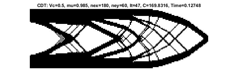
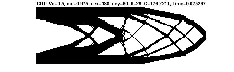
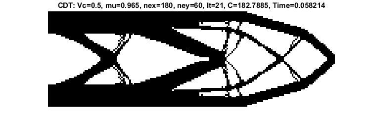
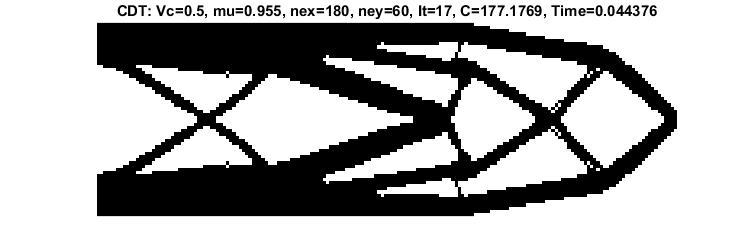
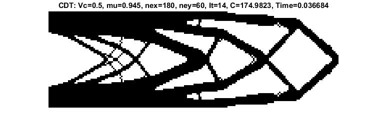
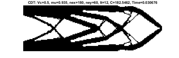
Figure 11: Experiment for volume reduction rate $\mu$ from $0.985$ (top) to $0.935$ (bottom)

By the fact that the alternative iteration is adopted in CDT method, the solution also depends sensitively on mesh resolution. Fig 12 shows the CDT solutions to the cantilever beam with different mesh resolutions from $20\times 8$ to $200\times 80$. Clearly, different mesh resolution leads to different topology. This is completely reasonable since different mesh size leads to totally different knapsack problem. Certainly, the finer is the mesh resolution, the better is the topology.

Figure 12: Experiment for mesh resolution from $20\times 8$ (top) to $200\times 80$ (bottom)

6.3 3-D Cantilever Beam

A CDT 3-D code (CDT3D) is developed based on the 169 line 3d topology optimization code (TOP3D) by Liu and Tovar [42]. Here we only provide a simple application to the cantilever beam. Since the BESO is not a polynomial-time algorithm, we only compare the CDT with the SIMP. The parameters in TOP3D are chosen to be penal=3, rmin=1.5. The volume reduction rate used in CDT3D is $\mu=0.95$.

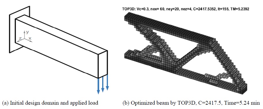
Figure 13: (a) 3-D cantilever beam and (b) SIMP solution

(a) CDT solution

(b) Front view

Figure 14: CDT solution and its front view

For a given volume fraction $\mu_{c}=0.3$, Fig. 14(b) shows the optimized beams by TOP3D. Figures 14 shows the solution by CDT3D.

Fig 15 shows the CDT3D solutions to the cantilever beam with $\mu=0.9$ and $\mu=0.94$, which verified again a truth in iteration method for solving a coupled optimization problem, i.e. the optimal solution depends strongly on the parameter $\mu$.

Figure 15: Experiment for volume reduction rates $\mu=0.9$ (top) and $\mu=0.94$ (bottom)

In order to have a closed look at inside of the 3-D beam, we increase the beam thickness from $nez=4$ to $nez=10$ and decrease the volume fraction from $\mu=0.5$ to $\mu_{c}=0.1$. Fig. 16 and Fig. 16 show results obtained by the TOP3D and CDT (with $\mu=0.93$) methods. We can see clearly that TOP3D produces many gray elements. While the optimal structure by the CDT is elegant and mechanically sound, also the computing time is three times faster.

(a) C=21427, Time=12.2

(b) Front view of SIMP solution

Figure 16: SIMP solution with $nez=10$ $\mu_{c}=0.1$

(a) C=13193, Time=4

(b) Front view of CDT solution

Figure 17: SIMP solution with $nez=10$, $\mu_{c}=0.1$ and $\mu=0.93$

7 Concluding remarks and open problems

Topology optimization has been studied via the canonical duality theory. Theoretical results presented in this paper show that this methodological theory is indeed powerful not only for solving the most challenging topology optimization problems, but also for correctly understanding and modeling multi-scale problems in complex systems. The numerical results verified that the CPD method can produce mechanically sound optimal topology, also it is much more faster than the popular SIMP and BESO methods. Specific conclusions are given below.

1. The mathematical problem for general topology optimization should be formulated as a bi-level knapsack programming $({\cal P}_{bk})$. This model works for both linearly and nonlinearly deformed elasto-plastic structures.

2. The CDT is a polynomial-time algorithm, which can solve general topology optimization problem to obtain global optimal solution at each volume iteration.

3. The $\beta$-perturbation for solving integer programming problems is actually the canonical penalty-duality method proposed in [13]. Theorem 3 is an application of the pure complementary energy principle in nonlinear elasticity [16]. This principle plays an important role not only in nonconvex analysis and computational mechanics, but also in topology optimization, especially for large deformed structures.

4. Unless a magic method is proposed, the volume reduction method is necessary for solving general knapsack-type problems if $\mu_{c}=V_{c}/V_{0}\ll 1$. But the global optimal solution depends sensitively on the reduction rate $\mu\in[\mu_{c},1)$.

5. The so-called compliance minimization problem $({\cal P}_{c})$ is actually a single-level reduction for solving $({\cal P}_{bk})$. Alternative iteration for the strain energy minimization $({\cal P}_{s})$ leads to an anti-knapsack problem, which has only trivial solution.

6. The problem $({\cal P}_{simp})$ is a box-constrained nonconvex minimization subjected to a knapsack condition. The SIMP is not a mathematically correct penalty method for solving either $({\cal P}_{c})$ or $({\cal P}_{s})$. Even if the magic number $p=3$ works for certain materials, this method can’t produce correct integer solutions for any given $p>1$.

7. The BESO method is actually a combination of the volume reduction and a direct method for solving the knapsack problem $({\cal P}_{kp})$. For small-scale problems, the BESO method can produce reasonable results better than by SIMP. But it is not a polynomial-time algorithm.

By the fact that the general topology optimization problem $({\cal P}_{bk})$ is a coupled, mixed integer nonlinear programming, although for each given lower-level solution $\mathbf{u}\in{\cal U}_{a}$ the upper-level problem can be solved analytically by the canonical duality theory, the final result produced by the CDT may not be the global optimal solution to $({\cal P}_{bk})$ since the alternative iterations for $\rho$ and $\mathbf{u}$ are adopted in Algorithm 1. This is the main reason why the numerical solution produced by the CDT depends on mesh resolution and volume reduction rate $\mu$. The main open problems include the optimal parameter $\mu$ in order to ensure the fast convergence rate with the optimal results, the influence of the mesh resolution to the optimal topology, the existence and uniqueness of a global optimization solution to $({\cal P}_{bk})$ for a given design domain $V_{c}$.

This paper is just a simple application of the canonical duality theory for linear elastic topology optimization. A 66-line Matlab code for topology optimization will be available soon to public. Also a refined algorithm with a 44-line Matlab code has been developed. The canonical duality theory is particularly useful for studying nonconvex, nonsmooth, nonconservative large deformed dynamical systems [19]. Therefore, the future works include the CDT method for solving general topology optimization problems of large deformed elasto-plastic structures subjected to dynamical loads.

Appendix: A Brief Review on Canonical Duality Theory

The canonical duality theory proposed in [18] comprises mainly

i) a canonical dual transformation,
ii) a complementary-dual principle, and
iii) a triality theory.

The canonical dual transformation is a versatile methodological method which can be used to model complex systems within a unified framework and to formulate perfect dual problems without a duality gap. The complementary-dual principle presents a unified analytic solution form for general problems in continuous and discrete systems. The triality theory reveals an intrinsic duality pattern in multi-scale systems, which can be used to identify both global and local extrema, and to develop deterministic algorithms for effectively solving a wide class of nonconvex/nonsmooth/discrete optimization/variational problems.

The canonical duality theory was developed from Gao and Strang’s original work [33] for solving the following nonconvex/nonsmooth variational problem

$$\inf\left\{\Pi(\mathbf{u})=\int_{\Omega}W(\nabla\mathbf{u}){{\rm d}\Omega}-F(\mathbf{u})\;|\;\;\mathbf{u}\in{\cal U}\right\},$$ (60)

where $F(\mathbf{u})$ is a generalized external energy, which is a linear functional of $\mathbf{u}$ on its effective domain ${\cal U}_{a}\subset{\cal U}$; the internal energy density $W(\mathbf{F})$ is the so-called super-potential in the sense of J.J. Moreau [50], which is a nonconvex/nonsmooth function of the deformation gradient $\mathbf{F}=\nabla\mathbf{u}$. Numerical discretization of (60) leads to a global optimization problem in finite dimensional space ${\cal X}\subset\mathbb{R}^{n}$. Canonical dual finite element method for solving the nonconvex/nonsmooth mechanics problem (60) was first proposed in 1996 [14].

Remark 4 (Objectivity and Conceptual Mistakes)

Objectivity is a central concept in our daily life, related to reality and truth. In philosophy, it means the state or quality of being true even outside a subject’s individual biases, interpretations, feelings, and imaginings. In science, the objectivity is often attributed to the property of scientific measurement, as the accuracy of a measurement can be tested independent from the individual scientist who first reports it. In continuum mechanics, a real-valued function $W:{\cal F}\subset\mathbb{R}^{n\times m}\rightarrow\mathbb{R}$ is called to be objective if

$$W(\mathbf{F})=W({\bf R}\mathbf{F})\;\;\forall\mathbf{F}\in{\cal F},\;\;\forall{\bf R},\;\;{\bf R}^{T}={\bf R}^{-1},\;\;\det{\bf R}=1.$$ (61)

The objectivity plays a fundamental rule in mathematical modeling, which is also called the principle of material frame indifference [52].

However, this important concept has been misused in optimization literature. As a result, the general problem in the so-called nonlinear programming is formulated as

$$\min f(x),\;\;s.t.\;\;h(x)=0,\;\;g(x)\leq 0,$$ (62)

where $f(x)$ is called the “objective function”, which is allowed to be any arbitrarily given function, even a linear function. Clearly, this mathematical problem is too abstract. Although it enables one to model a very wide range of problems, it comes at a price: many global optimization problems are considered to be NP-hard. Without detailed information on these arbitrarily given functions, it is impossible to have a powerful theory for solving the artificially given constrained problem (62). $\clubsuit$

In linguistics, a complete and grammatically correct sentence should be composed by at least three words: subject, object, and a predicate. As a language of science, the mathematics should follow this rule. Based on the excellent works by Oden-Reddy, Strang, and Tonti [52, 53, 62, 64], a general mathematical problem was proposed in [23]:

$$({\cal P}_{g}):\;\;\min\{\Pi(\mathbf{x})=W(\mathbf{D}\mathbf{x})-{F}(\mathbf{x})\;|\;\;\mathbf{x}\in{\cal X}\},$$ (63)

where $\mathbf{D}$ is a linear operator ($\nabla$ is a special case), which maps the configuration space ${\cal X}$ into a so-called intermediate space ${\cal W}$ [52, 53, 64]; $W:{\cal W}\rightarrow\mathbb{R}\cup\{+\infty\}$ is an objective function such that its sub-differential leads to the constitutive duality ${\bf w}^{*}\in\partial^{-}W({\bf w})\subset{\cal W}^{*}$, which is governed by the constitutive law and all possible physical constraints; while ${F}:{\cal X}\rightarrow\mathbb{R}\cup\{-\infty\}$ is a so-called subjective function such that its over-differential leads to the action-reaction duality $\mathbf{x}^{*}\in\partial^{+}{F}(\mathbf{x})\subset{\cal X}^{*}$ including all possible boundary conditions and geometrical constraints [17]. This subjective function must be linear on its effective domain ${\cal X}_{a}=\{\mathbf{x}\in{\cal X}|\;\;{F}(\mathbf{x})>-\infty\}$, i.e. ${F}(\mathbf{x})=\langle\mathbf{x},\mathbf{f}\rangle\;\;\forall\mathbf{x}\in{\cal X}_{a}$, where $\mathbf{f}\in{\cal X}^{*}$ is an given action, the feasible set ${\cal X}_{a}$ includes all possible geometrical constraints. The predicate in $({\cal P}_{g})$ is the operator “$-$” and the difference $\Pi(\mathbf{x})$ is called the target function in general problems. The object and subject are in balance only at the optimal states. By the fact that ${\cal X}$ and ${\cal W}$ can be in different dimensional spaces, this unified problem can be used to model multi-scale systems [18, 34].

The unified form $({\cal P}_{g})$ covers general constrained nonconvex/nonsmooth/discrete variational and optimization problems in multi-scale complex systems [27, 34] as well as all equilibrium problems in linear elasto-plasticity and mathematical physics [53, 62].

Definition 1 (Properly and Well-Posed Problems)

A problem is called properly posed if for any given non-trivial input it has at least one non-trivial solution. It is called well-posed if the solution is unique.

Clearly, this definition is more general than Hadamard’s well-posed problems in dynamic systems since the continuity condition is not included. Physically speaking, any real-world problems should be well-posed since all natural phenomena exist uniquely. But practically, it is difficult to model a real-world problem precisely. Therefore, properly posed problems are allowed for the canonical duality theory. This definition is important for understanding the triality theory and NP-hard problems.

It is well-known in finite deformation theory that the stored energy $W(\mathbf{F})$ is an objective function if and only if there exists an objective strain tensor $\mathbf{C}=\mathbf{F}^{T}\mathbf{F}$ and a function $U(\mathbf{C})$ such that $W(\mathbf{F})=U(\mathbf{C})$ [10]. In nonlinear elasticity, the function $U(\mathbf{C})$ is usually convex (say the St Venant-Kirchhoff material) such that the duality relation $\mathbf{C}^{*}\in\partial U(\mathbf{C})$ is invertible and the complementary energy $U^{*}(\mathbf{C}^{*})$ can be uniquely defined via the Legendre-Fenchel transformation $U^{*}(\mathbf{C}^{*})=\sup_{\mathbf{C}}\{\mathbf{C}:\mathbf{C}^{*}-U(\mathbf{C})\}$. These basic truths in continuum physics laid a foundation for the canonical duality theory.

The key idea of the canonical transformation is to introduce a nonlinear operator $\mbox{\boldmath$\xi$}=\Lambda(\mathbf{x}):{\cal X}\rightarrow{\cal E}$ and a convex, lower semi-continuous function $\Psi(\mbox{\boldmath$\xi$}):{\cal E}\rightarrow\mathbb{R}\cup\{+\infty\}$ such that the nonconvex function $W(\mathbf{D}\mathbf{x})$ can be written in the canonical form

$$W(\mathbf{D}\mathbf{x})=\Psi(\Lambda(\mathbf{x}))\;\;\forall\mathbf{x}\in{\cal X}$$ (64)

and the following canonical duality relations hold

$$\mbox{\boldmath$\varsigma$}\in\partial\Psi(\mbox{\boldmath$\xi$})\;\;\Leftrightarrow\;\;\mbox{\boldmath$\xi$}\in\partial\Psi^{*}(\mbox{\boldmath$\varsigma$})\;\;\Leftrightarrow\;\;\Psi(\mbox{\boldmath$\xi$})+\Psi^{*}(\mbox{\boldmath$\varsigma$})=\langle\mbox{\boldmath$\xi$};\mbox{\boldmath$\varsigma$}\rangle,$$

where $\langle\mbox{\boldmath$\xi$};\mbox{\boldmath$\varsigma$}\rangle$ represents the bilinear form on ${\cal E}$ and its canonical dual ${\cal E}^{*}$. Thus, using the Fenchel-Young equality $\Psi(\mbox{\boldmath$\xi$})=\langle\mbox{\boldmath$\xi$};\mbox{\boldmath$\varsigma$}\rangle-\Psi^{*}(\mbox{\boldmath$\varsigma$})$, the nonconvex/nonsmooth minimization problem (63) can be equivalently written in the following min-max form

$$\min_{\mathbf{x}\in{\cal X}}\max_{\mbox{\boldmath$\varsigma$}\in{\cal E}^{*}}\{\Xi(\mathbf{x},\mbox{\boldmath$\varsigma$})=\langle\Lambda(\mathbf{x});\mbox{\boldmath$\varsigma$}\rangle-\Psi^{*}(\mbox{\boldmath$\varsigma$})-{F}(\mathbf{x})\},$$ (65)

where $\Xi(\mathbf{x},\mbox{\boldmath$\varsigma$})$ is the so-called total complementary function, first introduced by Gao and Strang in 1989 [33]. Particularly, if $\mbox{\boldmath$\varepsilon$}=\Lambda(\mathbf{x})$ is a homogeneous quadratic operator, then $\langle\Lambda(\mathbf{x});\mbox{\boldmath$\varsigma$}\rangle=\frac{1}{2}\mathbf{x}^{T}\mathbf{G}(\mbox{\boldmath$\varsigma$})\mathbf{x}=G_{ap}(\mathbf{x},\mbox{\boldmath$\varsigma$})$ is the so-called complementary gap function, where the Hessian matrix $\mathbf{G}(\mbox{\boldmath$\varsigma$})=\nabla^{2}_{\mathbf{x}}G_{ap}(\mathbf{x},\mbox{\boldmath$\varsigma$})$ depends on the quadratic operator $\Lambda(\mathbf{x})$. This gap function recovers the duality gap produced by the traditional Lagrange multiplier method and modern Fenchel-Moreau duality theory. By using $\Xi$, the canonical dual function $\Pi^{d}(\mbox{\boldmath$\varsigma$})$ can be obtained as [21]

$$\Pi^{d}(\mbox{\boldmath$\varsigma$})=\mbox{sta}\{\Xi(\mathbf{x},\mbox{\boldmath$\varsigma$})|\;\;\mathbf{x}\in{\cal X}_{a}\;\}=-\frac{1}{2}\langle[\mathbf{G}(\mbox{\boldmath$\varsigma$})]^{+}\mathbf{f},\mathbf{f}\rangle-\Psi^{*}(\mbox{\boldmath$\varsigma$}),$$ (66)

where $\mbox{sta }\{f(x)|\;x\in X\}$ stands for finding a stationary value of $f(x),\ \forall x\in X$, and $\mathbf{G}^{+}$ represents a generalized inverse of $\mathbf{G}$. Based on this canonical dual function, a general solution to the nonconvex problem (63) can be obtained [17].

Theorem 5 (Complementary-Dual Principle and Analytic Solution)

  For a given input $\mathbf{f}\in{\cal X}^{*}$, the vector $\bar{\mathbf{x}}=[\mathbf{G}(\bar{\mbox{\boldmath$\varsigma$}})]^{+}\mathbf{f}$ is a stationary point of $\Pi(\mathbf{x})$ if and only if $\bar{\mbox{\boldmath$\varsigma$}}$ is a stationary point of $\Pi^{d}(\mbox{\boldmath$\varsigma$})$, $(\bar{\mathbf{x}},\bar{\mbox{\boldmath$\varsigma$}})$ is a stationary point of $\Xi(\mathbf{x},\mbox{\boldmath$\varsigma$})$, and $\Pi(\bar{\mathbf{x}})=\Xi(\bar{\mathbf{x}},\bar{\mbox{\boldmath$\varsigma$}})=\Pi^{d}(\bar{\mbox{\boldmath$\varsigma$}})$

This theorem was first proposed in 1997 for a large deformed beam theory [15]. In nonlinear elasticity, the canonical dual function $\Pi^{d}(\mbox{\boldmath$\varsigma$})$ is the so-called pure complementary energy, first proposed in 1999 [16]. This principle solved a 50-year old open problem in finite deformation theory and is known as the Gao principle in literature [47]. Clearly, $\mbox{\boldmath$\varsigma$}\in{\cal S}^{+}_{a}$ if and only if $G_{ap}(\mathbf{x},\mbox{\boldmath$\varsigma$})\geq 0\;\;\forall\mathbf{x}\in{\cal X}_{a}$. The following triality theory shows that this gap function provides a global optimality criterion in nonconvex mechanics and global optimization.

Theorem 6 (Triality Theory [17])

Suppose that $(\bar{\mathbf{x}},\bar{\mbox{\boldmath$\varsigma$}})$ is a stationary solution of $\Xi(\mathbf{x},\mbox{\boldmath$\varsigma$})$ and ${\cal X}_{o}\times{\cal S}_{o}$ is a neighborhood of $\left(\bar{\mathbf{x}},\bar{\mbox{\boldmath$\varsigma$}}\right)$.

If $\bar{\mbox{\boldmath$\varsigma$}}\in{\cal S}^{+}_{a}=\{\mbox{\boldmath$\varsigma$}\in{\cal E}^{*}|\;\;\mathbf{G}(\mbox{\boldmath$\varsigma$})\succeq 0\}$, then

$$\Pi(\bar{\mathbf{x}})=\min_{\mathbf{x}\in{\cal X}_{a}}\Pi\left(\mathbf{x}\right)=\max_{\mbox{\boldmath$\varsigma$}\in{\cal S}^{+}_{a}}\Pi^{d}\left(\mbox{\boldmath$\varsigma$}\right)=\Pi^{d}(\bar{\mbox{\boldmath$\varsigma$}}).\vspace{-.1cm}$$ (67)

If $\bar{\mbox{\boldmath$\varsigma$}}\in{\cal S}^{-}_{a}=\{\mbox{\boldmath$\varsigma$}\in{\cal E}^{*}|\;\;\mathbf{G}(\mbox{\boldmath$\varsigma$})\prec 0\}$, then we have either

$$\Pi(\bar{\mathbf{x}})=\max_{\mathbf{x}\in{\cal X}_{o}}\Pi\left(\mathbf{x}\right)=\max_{\mbox{\boldmath$\varsigma$}\in{\cal S}_{o}}\Pi^{d}\left(\mbox{\boldmath$\varsigma$}\right)=\Pi^{d}(\bar{\mbox{\boldmath$\varsigma$}}),\vspace{-.1cm}$$ (68)

or (if $\dim\Pi=\dim\Pi^{d}$)

$$\Pi(\bar{\mathbf{x}})=\min_{\mathbf{x}\in{\cal X}_{o}}\Pi\left(\mathbf{x}\right)=\min_{\mbox{\boldmath$\varsigma$}\in{\cal S}_{o}}\Pi^{d}\left(\mbox{\boldmath$\varsigma$}\right)=\Pi^{d}(\bar{\mbox{\boldmath$\varsigma$}}).\vspace{-.1cm}$$ (69)

This triality theory shows that the Gao-Strang gap function can be used to identify both global minimizer and the biggest local extrema. To understand the canonical duality theory, let us consider a simple nonconvex optimization in $\mathbb{R}^{n}$:

$$\min\left\{\Pi(\mathbf{x})=\frac{1}{2}\beta(\frac{1}{2}\|\mathbf{x}\|^{2}-\lambda)^{2}-\mathbf{x}^{T}\mathbf{f}\;\;\;\forall\mathbf{x}\in\mathbb{R}^{n}\right\},$$ (70)

where $\alpha,\lambda>0$ are given parameters. The criticality condition $\nabla\Pi(\mathbf{x})=0$ leads to a nonlinear algebraic equation system $\beta(\frac{1}{2}\|\mathbf{x}\|^{2}-\lambda)\mathbf{x}=\mathbf{f}.$ Clearly, this n-dimensional nonlinear algebraic equation may have multiple solutions. Due to the nonconvexity, traditional convex optimization theories can’t be used to identify global minimizer. However, by the canonical dual transformation, this problem can be solved completely to obtain all extremum solutions. To do so, we let $\xi=\Lambda(\mathbf{x})=\frac{1}{2}\|\mathbf{x}\|^{2}\in\mathbb{R}$. Then, the nonconvex function $W(\mathbf{x})=\frac{1}{2}\beta(\frac{1}{2}\|\mathbf{x}\|^{2}-\lambda)^{2}$ can be written in canonical form $\Psi(\xi)=\frac{1}{2}\beta(\xi-\lambda)^{2}$. Its Legendre conjugate is given by $\Psi^{*}(\varsigma)=\frac{1}{2}\beta^{-1}\varsigma^{2}+\lambda\varsigma$, which is strictly convex. Thus, the total complementary function for this nonconvex optimization problem is

$$\Xi(\mathbf{x},\varsigma)=\frac{1}{2}\|\mathbf{x}\|^{2}\varsigma-\lambda\varsigma-\frac{1}{2}\beta^{-1}\varsigma^{2}-\mathbf{x}^{T}\mathbf{f}.$$ (71)

For a fixed $\varsigma\in\mathbb{R}$, the criticality condition $\nabla_{\mathbf{x}}\Xi(\mathbf{x},\varsigma)=0$ leads to $\varsigma\mathbf{x}-\mathbf{f}=0.$ So the analytical solution $\mathbf{x}=\varsigma^{-1}\mathbf{f}$ holds for $\varsigma\neq 0$. Substituting this into the total complementary function $\Xi$, the canonical dual function can be easily obtained as

$$\Pi^{d}(\varsigma)=\{\Xi(\mathbf{x},\varsigma)|\nabla_{\mathbf{x}}\Xi(\mathbf{x},\varsigma)=0\}=-\frac{\|\mathbf{f}\|^{2}}{2\varsigma}-\frac{1}{2}\beta^{-1}\varsigma^{2}-\lambda\varsigma,\;\;\;\forall\varsigma\neq 0.$$ (72)

The critical point of this canonical function is obtained by solving the following dual algebraic equation

$$(\beta^{-1}\varsigma+\lambda)\varsigma^{2}=\frac{1}{2}\|\mathbf{f}\|^{2}.$$ (73)

For any given parameters $\beta$, $\lambda$ and the vector $\mathbf{f}\neq{\bf 0}\in\mathbb{R}^{n}$, this cubic algebraic equation has three non trivial real solutions $\varsigma_{1}\in{\cal S}^{+}_{a}=\{\varsigma\in\mathbb{R}\;|\;\varsigma<0\}$, $\varsigma_{2,3}\in{\cal S}^{-}_{a}=\{\varsigma\in\mathbb{R}\;|\;\varsigma<0\}$, then triality theory tells us that $\mathbf{x}_{1}=\mathbf{f}/\varsigma_{1}$ is a global minimizer, $\mathbf{x}_{2}=\mathbf{f}/\varsigma_{2}$ is a local minimizer, $\mathbf{x}_{3}=\mathbf{f}/\varsigma_{3}$ is a local maximizer of $\Pi(\mathbf{x})$, and $\Pi(\mathbf{x}_{i})=\Pi^{d}(\varsigma_{i}),\;i=1,2,3$ (see Fig 18).

(a) $f=0.5$

(b) $f=0$

Figure 18: Graphs of $\Pi(\mathbf{x})$ (solid) and $\Pi^{d}(\varsigma)$ (dashed) for $n=1,\;\;\beta=1,\;\;\lambda=2$ with $x_{1}=2.1$, $\varsigma_{1}=0.24$ and $\Pi(x_{1})=-1.02951=\Pi^{d}(\varsigma_{1})$ (see the two black dots in (a)) if $f=0.5$. While $x_{1,2}=\pm 2$ if $f=0$ (see (b)).

If $\mathbf{f}=0$, the graph of $\Pi(\mathbf{x})$ is symmetric (i.e. the so-called double-well potential or the Mexican hat for $n=2$ [17]) with infinite number of global minimizers satisfying $\|\mathbf{x}\|^{2}=2\lambda$. In this case, the canonical dual $\Pi^{d}(\varsigma)=-\frac{1}{2}\beta^{-1}\varsigma^{2}-\lambda\varsigma$ is strictly concave with only one critical point (local maximizer) $\varsigma_{3}=-\beta\lambda<0$ (for $\beta,\lambda>0$). The corresponding solution $\mathbf{x}_{3}=\mathbf{f}\varsigma_{3}=0$ is a local maximizer and $\Pi(\mathbf{x}_{3})=\Pi^{d}(\varsigma_{3})$. By the canonical dual equation (73) we have $\varsigma_{1}=\varsigma_{2}=0$ located on the boundary of ${\cal S}^{+}_{a}$. In this case, the analytical solution $\mathbf{x}=\mathbf{f}/\varsigma$ is singular. For $n=1$, these two roots are corresponding to the two global minimizers $x_{1,2}=\pm\sqrt{2\lambda}$ (see Fig. 18 (b)), which can be obtained by linear perturbation.

This simple example reveals a fundament truth in global optimization, i.e., for a given nonconvex/discrete minimization problem in ${\cal X}\subset\mathbb{R}^{n}$, its canonical dual is a concave maximization over a convex set ${\cal S}^{+}_{a}\subset\mathbb{R}^{m}$, which can be solved easily to obtain a unique solution if ${\cal S}^{+}_{a}$ has no-empty interior. Very often $n\gg m$. Otherwise, the primal problem could be really NP-hard. Therefore, the canonical duality theory can be used to identify if a global optimization problem is not NP-hard. Generally speaking, if a non-symmetrically distributed external force $\mathbf{f}\neq 0$, the canonical dual feasible set ${\cal S}^{+}_{a}$ has no-empty interior. It was proved in [21] that for quadratic 0-1 integer programming problem, if the source term $\mathbf{f}$ is bigger enough, the solution is simply $\{x_{i}\}=\{0\mbox{ if }f_{i}<0,\;1\;\mbox{ if }f_{i}>0\}$ (Theorem 8, [21]). The canonical duality theory has been used successfully for solving a large class of challenging problems in multidisciplinary fields of engineering and sciences. A comprehensive review and applications are given in the recent book [27].

Mathematics and mechanics have been complementary partners since the Newton times. Many fundamental ideas, concepts, and mathematical methods extensively used in calculus of variations and optimization are originally developed from mechanics. The canonical duality theory is a typical example developed from Gao and Strang’s work on finite deformation theory, where the subjective function $F(\mathbf{u})$ must be linear so that the input force $\mathbf{f}=\partial F(\mathbf{u})$ is independent of $\mathbf{u}$ (i.e. a dead-load). Dually, the objective function $W(\mbox{\boldmath$\epsilon$})$ must be nonlinear such that there exists an objective measure $\mbox{\boldmath$\xi$}=\Lambda(\mathbf{u})$ and a convex function $\Psi(\mbox{\boldmath$\xi$})$, the canonical transformation $W(\mathbf{D}\mathbf{u})=\Psi(\Lambda(\mathbf{u}))$ holds for most real-world systems. This is the reason why the canonical duality theory can be used naturally to solve general challenging problems in multidisciplinary fields. However, the objectivity has been misused in engineering optimization. As a consequence, the subjective function $F(\mathbf{u})=\mathbf{u}^{T}\mathbf{f}$ has been extensively used as the objective function in topology optimization, the minimum compliance problem $({\cal P}_{c})$ has been mistakenly written as the minimum strain energy problem $({\cal P}_{s})$, and the stored energy $W(\mathbf{D}\mathbf{u})=\frac{1}{2}\mathbf{u}^{T}\mathbf{K}(\mbox{\boldmath$\rho$})\mathbf{u}$ has been confusedly called the mean compliance. Also, the objectivity has been misused in mathematical optimization. It turns out the canonical duality theory has been mistakenly challenged by M.D. Voisei and C. Z$\breve{a}$linescu in several publications (cf. [27]). By oppositely choosing linear functions for $W(\mbox{\boldmath$\epsilon$})$ and nonlinear functions for $F(\mathbf{u})$, they produced a list of “count-examples” and concluded: “a correction of this theory is impossible without falling into trivial”. The conceptual mistakes in these challenges as well as in topology optimization revealed at least two important issues: 1) there exists a big gap between optimization and mechanics; 2) incorrectly using the well-defined concepts can lead to not only ridiculous arguments, but also wrong mathematical model. As V.I. Arnold indicated [3]: “In the middle of the twentieth century it was attempted to divide physics and mathematics. The consequences turned out to be catastrophic”. Interested readers are recommended to read the recent papers [22, 31] for further discussion.

References

- [1] G. Allaire, F. Jouve, and A.M. Toader. A level-set method for shape optimization. Comptes Rendus Mathematique, 334(12):1125–1130, 2002.
- [2] E. Andreassen, A. Clausen, M. Schevenels, B. S. Lazarov, and O. Sigmund. Efficient topology optimization in MATLAB using 88 lines of code. Structural and Multidisciplinary Optimization, 43(1):1–16, 2011.
- [3] V.I. Anorld. On teaching mathematics. Russian Math. Surveys, 53(1):229–236, 1998.
- [4] M. Beckers. Topology optimization using a dual method with discrete variales. Structural Optimization, 17(1):14–24, 1999.
- [5] M. Beckers. Dual methods for discrete structural optimization problems. International Journal for Numerical Methods in Engineering, 48(12):1761–1784, 2000.
- [6] M.P. Bendsoe. Optimal shape design as a material distribution problem. Structural Optimization, 1:193–202, 1989.
- [7] M.P. Bendsoe and N. Kikuchi. Generating optimal topologies in structural design using a homogenization method. Computer Methods in Applied Mechanics and Engineering, 72(2):197–224, 1988.
- [8] R.S. Burachik, W.P. Freire, and C.Y. Kaya. Interior epigraph directions method for nonsmooth and nonconvex optimization via generalized augmented lagrangian duality. J. Global Optimization, 60:501–529, 2014.
- [9] Y. Chen and D.Y. Gao. Global solutions to spherical constrained quadratic minimization via canonical duality theory. In DY Gao, V. Latorre, and N. Ruan, editors, Canonical Duality Theory: Unified Methodology for Multidisciplinary Study. Spinger, New York, 2017.
- [10] P.G. Ciarlet. Linear and Nonlinear Functional Analysis with Applications. Society for Industrial and Applied Mathematics, 2013.
- [11] Xiaotie Deng. Complexity issues in bilevel linear programming. Multilevel optimization: Algorithms and applications, pages 149–164, 1998.
- [12] A. Díaz and O. Sigmund. Checkerboard patterns in layout optimization. Structural Optimization, 10(1):40–45, 1995.
- [13] D.Y. Gao. Panpenalty finite element programming for plastic limit analysis. Computers & Structures, 28(6):749–755, 1988.
- [14] D.Y. Gao. Complementary finite-element method for finite deformation nonsmooth mechanics. Journal of Engineering Mathematics, 30(3):339–353, 1996.
- [15] D.Y. Gao. Dual extremum principles in finite deformation thoery with applications to post-buckling analysis of extended nonlinear beam model. Applied Mechanics Reviews, 50:S64–S71, 1997.
- [16] D.Y. Gao. Pure complementary energy principle and triality theory in finite elasticity. Mechanics Research Communications, 26(1):31–37, 1999.
- [17] D.Y. Gao. Canonical dual transformation method and generalized triality theory in nonsmooth global optimization. Journal of Global Optimization, 17(1):127–160, 2000.
- [18] D.Y. Gao. Duality Principles in Nonconvex Systems: Theory, Methods, and Applications. Springer, New York, 2000.
- [19] D.Y. Gao. Complementarity, polarity and triality in nonsmooth, nonconvex and nonconservative hamilton systems. Philosophical Transactions of the Royal Society: Mathematical, Physical and Engineering Sciences, 359:2347–2367, 2001.
- [20] D.Y. Gao. Solutions and optimality criteria to box constrained nonconvex minimization problems. Journal of Industrial & Management Optimization, 3(2):293–304, 2007.
- [21] D.Y. Gao. Canonical duality theory: Unified understanding and generalized solution for global optimization problems. Computers & Chemical Engineering, 33(12):1964–1972, 2009.
- [22] DY Gao. On unified modeling, canonical duality-triality theory, challenges and breakthrough in optimization,. https://arxiv.org/abs/1605.05534, 2016.
- [23] D.Y. Gao. On unified modeling, theory, and method for solving multi-scale global optimization problems,. In D. E. Kvasov Y. D. Sergeyev and M. S. Mukhametzhanov, editors, Numerical Computations: Theory And Algorithms. AIP Conference Proceedings, vol. 1776, 020005, 2016.
- [24] D.Y. Gao. Canonical duality theory for topology optimization. In DY Gao, V. Latorre, and N. Ruan, editors, Canonical Duality Theory: Unified Methodology for Multidisciplinary Study, pages 263–276. Spinger, New York, 2017.
- [25] D.Y. Gao. Canonical duality-triality: Unified understanding modeling, problems, and np-hardness in multi-scale optimization. In VK Singh, DY Gao, and A. Fisher, editors, Emerging Trends in Applied Mathematics and Hi-Perfermance Computingy. Spinger, New York, 2018.
- [26] D.Y. Gao and E.J. Ali. A novel canonical duality theory for solving 3-d topology optimization problems. In V.K. Singh, DY Gao, and A. Fisher, editors, Emerging Trends in Applied Mathematics and High-Performence Computing, 2018.
- [27] DY Gao, V Latorre, and N Ruan. Canonical Duality Theory: Unified Methodology for Multidisciplinary Study. Spriner, New York, 2017.
- [28] D.Y. Gao and D. Motreanu. Handbook of Nonconvex Analysis and Applications. International Press, Boston, 2010.
- [29] D.Y. Gao and R.W. Ogden. Multi-solutions to non-convex variational problems with implications for phase transitions and numerical computation. Q. J. Mech. Appl. Math., 61:497–522, 2008.
- [30] D.Y. Gao and N. Ruan. Solutions to quadratic minimization problems with box and integer constraints. Journal of Global Optimization, 47(3):463–484, 2010.
- [31] D.Y. Gao, N. Ruan, and V. Latorre. Canonical duality-triality: Bridge between nonconvex analysis/mechanics and global optimization in complex systems. In DY Gao, V. Latorre, and N. Ruan, editors, Canonical Duality Theory: Unified Methodology for Multidisciplinary Study. Spinger, 2017.
- [32] D.Y. Gao, N. Ruan, and H.D. Sherali. Solutions and optimality criteria for nonconvex constrained global optimization problems with connections between canonical and lagrangian duality. Journal of Global Optimization, 45(3):473–497, 2009.
- [33] D.Y. Gao and Gilbert Strang. Geometric nonlinearity: Potential energy, complementary energy, and the gap function. Quarterly Applied Math, 47(3):487–504, 1989.
- [34] D.Y. Gao and H.F. Yu. Multi-scale modelling and canonical dual finite element method in phase transitions of solids. Int. J. Solids Struct., 45:3660–3673, 2008.
- [35] P. Hansen, B. Jaumard, and G. Savard. New branch-and-bound rules for linear bilevel programming. SIAM Journal on Scientific and Statistical Computing, 13:1194–1217, 1992.
- [36] X. Huang and Y. M. Xie. Evolutionary topology optimization of geometrically and materially nonlinear structures under prescribed design load. Structural Engineering and Mechanics, 34(5):581–595, 2010.
- [37] X. Huang and Y.M. Xie. A further review of ESO type methods for topology optimization. Structural and Multidisciplinary Optimization, 41:671–683, 2010.
- [38] G. Isac. Complementarity Problems. Springer, 1992.
- [39] C. S. Jog. A robust dual algorithm for topology design of structures in discrete variables. International Journal for Numerical Methods in Engineering, 50(7):1607–1618, 2001.
- [40] C. S. Jog. Topology design of structures using a dual algorithm and a constraint on the perimeter. International Journal for Numerical Methods in Engineering, 54(7):1007–1019, 2002.
- [41] C. S Jog. A dual algorithm for the topology optimization of nonlinear elastic structures. International Journal for Numerical Methods in Engineering, 77(4):502–517, 2010.
- [42] A. Tovar K. Liu. An efficient 3d topology optimization code written inmatlab. Struct Multidisc Optim, 50:1175–1196, 2014.
- [43] Richard M. Karp. Reducibility among combinatorial problems. In R. E. Miller and J. W. Thatcher, editors, Complexity of Computer Computations, pages 85–103, New York: Plenum, 1972.
- [44] V. Latorre and D.Y. Gao. Canonical duality for solving general nonconvex constrained problems. Optimization Letters, 10:1763–1779, 2016.
- [45] V. Latorre and D.Y. Gao. Global optimal trajectory in chaos and np-hardness. Int. J. Birfucation and Chaos, 26:1650142, 2016.
- [46] Jon Lee and Sven Leyffer. Mixed Integer Nonlinear Programming. Springer, 2012.
- [47] S.F. Li and A. Gupta. On dual configuration forces. J. of Elasticity, 84:13–31., 2006.
- [48] P. Manyem. Computational complexity, np-completeness and optimization duality: A survey. https://arxiv.org/pdf/1012.5568.pdf arXiv:1012.5568v2, 15 Nov 2011.
- [49] C. Mattheck and S. Burkhardt. A new method of structural shape optimization based on biological growth. International Journal of Fatigue, 12(3):185–190, 1990.
- [50] J.J. Moreau. La notion de sur-potentiel et les liaisons unilatérales en élastostatique. CR Acad. Sc. Paris, 267:954–957, 1968.
- [51] D. Morelas and D.Y. Gao. On minimal distance between two surfaces. In DY Gao, V. Latorre, and N. Ruan, editors, Canonical Duality Theory: Unified Methodology for Multidisciplinary Study, pages 359–372. Spinger, 2017.
- [52] J.T. Oden. An Introduction to Mathematical Modeling. John Wiley & Sons, 2011.
- [53] J.T. Oden and J.N. Reddy. Variational Methods in Theoretical Mechanics. Springer-Verlag, 1983.
- [54] P.M. Pardalos and S.A Vavasis. Quadratic programming with one negative eigenvalue is np-hard. Journal of Global Optimization, 1:15–22, 1991.
- [55] G.I. N. Rozvany. A critical review of established methods of structural topology optimization. Structural and Multidisciplinary Optimization, 37:217–237, 2009.
- [56] O. Sigmund and K. Maute. Topology optimization approaches: a comparative review. Structural and Multidisciplinary Optimization, 48(6):1031–1055, 2013.
- [57] O. Sigmund and J. Petersson. Numerical instabilities in topology optimization: A survey on procedures dealing with checkerboards, mesh-dependencies and local minima. Structural Optimization, 16(1):68–75, 1998.
- [58] A. Sinha, P. Malo, and K. Deb. A Review on Bilevel Optimization: From Classical to Evolutionary Approaches and Applications. 2017.
- [59] J. Sokolowski and A. Zochowski. On the topological derivative in shape optimization. Structural Optimization, 37:1251–1272, 1999.
- [60] M. Stolpe and K. Svanberg. On the trajectories of penalization methods for topology optimization. Structural and Multidisciplinary Optimization, 21(2):128–139, 2001.
- [61] M. Stolpe and K. Svanberg. Modelling topology optimization problems as linear mixed 0-1 programs. International Journal for Numerical Methods in Engineering, 57(5):723–739, 2003.
- [62] G. Strang. Introduction to Applied Mathematics. Wellesley-Cambridge Press, 1986.
- [63] K. Suresh. A 199-line Matlab code for Pareto-optimal tracing in topology optimization. Structural and Multidisciplinary Optimization, 42(5):665–679, 2010.
- [64] Enzo Tonti. The Mathematical Structure of Classical and Relativistic Physics. Birkh’auser, 2013.
- [65] L. Vicente, G. Savard, and J. Júdice. Descent approaches for quadratic bilevel programming. Journal of Optimization Theory and Applications, 81:379––399, 1994.
- [66] M.Y. Wang, X. Wang, and D. Guo. A level set method for structural topology optimization. Computer Methods in Applied Mechanics and Engineering, 192(1-2):227–246, 2003.
- [67] Z.B. Wang, S.C. Fang, D.Y. Gao, and W.X. Xing. Canonical dual approach to solving the maximum cut problem. J. Glob. Optim., 54:341–351, 2012.
- [68] Y.M. Xie and G.P. Steven. A simple evolutionary procedure for structural optimization. Comput Struct, 49:885–896, 1993.
- [69] M. Zhou and G. I. N. Rozvany. The COC algorithm, part II: Topological, geometrical and generalized shape optimization. Computer Methods in Applied Mechanics and Engineering, 89(1-3):309–336, 1991.