Learning Free Energy Landscapes Using Artificial Neural Networks

Abstract

Existing adaptive bias techniques, which seek to estimate free energies and physical properties from molecular simulations, are limited by their reliance on fixed kernels or basis sets which hinder their ability to efficiently conform to varied free energy landscapes. Further, user-specified parameters are in general non-intuitive, yet significantly affect the convergence rate and accuracy of the free energy estimate. Here we propose a novel method wherein artificial neural networks (ANNs) are used to develop an adaptive biasing potential which learns free energy landscapes. We demonstrate that this method is capable of rapidly adapting to complex free energy landscapes and is not prone to boundary or oscillation problems. The method is made robust to hyperparameters and overfitting through Bayesian regularization which penalizes network weights and auto-regulates the number of effective parameters in the network. ANN sampling represents a promising innovative approach which can resolve complex free energy landscapes in less time than conventional approaches while requiring minimal user input.

I Introduction

Use of adaptive biasing methods to estimate free energies of relevant chemical processes from molecular simulation has gained popularity in recent years. Free energy calculations have become central to the computational study of biomolecular systems Barducci et al. (2013), material properties Joshi et al. (2014), and rare events Valsson et al. (2016). The metadynamics algorithm Laio and Parrinello (2002), which uses a sum of Gaussian kernels to obtain a free energy landscape (FEL) on-the-fly, has unleashed a groundswell of new activity studying on–the–fly approximations of FELs. Many extensions of this method have been proposed Barducci et al. (2008); Singh et al. (2011); Dama et al. (2014); Valsson et al. (2016), which enhance the speed and accuracy of metadynamics simulations, though the essential limitation—representing the FEL with Gaussians—has remained. Notably, the optimal choice of parameters such as the multidimensional Gaussian widths, height and deposition rate are unknown for each new system and poor choices can severely affect both the convergence rate and the accuracy of the estimated FEL. Partial remedies involving locally optimized bias kernels exist Branduardi et al. (2012); Barducci et al. (2008), though these cannot correct for systematic limitations inherent to the approximation of a surface by Gaussians, including boundary errors McGovern and De Pablo (2013).

Inspired by adaptive bias umbrella sampling Mezei (1987); Hooft et al. (1992); Bartels and Karplus (1997, 1998), algorithms have begun to emerge which address these limitations, including variationally enhanced sampling (VES) Valsson and Parrinello (2014), basis function sampling (BFS) Whitmer et al. (2014), and Green’s function sampling (GFS) Whitmer et al. (2015). Each utilizes orthogonal basis expansions to represent the underlying FEL, with VES deriving a variational functional which, when stochastically minimized, yields the optimal expansion coefficients. The related BFS approximates FELs using a probability density obtained through an accumulated biased histogram, and determines the coefficients by direct projection of the data onto a chosen orthogonal basis set. GFS, a dynamic version of BFS, invokes a metadynamics-like algorithm approximating a delta function, resulting in a trajectory which reveals optimal coefficients on-the-fly. The basis expansions employed by these methods, which can represent the often nuanced and highly nonlinear FELs more robustly than Gaussians, also benefit by eliminating the need for kernel-specific properties such as width and height. A user must still specify the number of terms to include in the expansion and “deposition rate” parameters which control the aggressiveness of bias updating. Still, there remain a number of non–ideal practical and theoretical issues which must be addressed. Importantly, the use of any functional form to represent the FEL inherits both the advantages and disadvantages of that set of functions. Basis sets, for example, may lead to Runge or Gibbs phenomena on sharply varying surfaces or near boundaries. These characteristic oscillations introduce artificial free energy barriers which may prevent the system from sampling important regions of phase space, and result in a non-converging bias. These do not self-correct, and increasing the order of the expansion is generally not helpful Kincaid and Cheney (2009).

Alternative algorithms, while less prevalent in the literature, nonetheless exhibit many benefits. Adaptive biasing force (ABF) methods Darve and Pohorille (2001), developed in parallel to metadynamics-derived methods, seek to estimate the underlying mean force (rather than the free energy) at discrete points along the coordinates of interest. The mean force is then integrated at the end of a simulation to obtain the corresponding FEL. The primary advantage of ABF over biasing potential approaches is the local nature of the mean force at a given point. While the free energy is a global property related the to probability distribution along a set of coordinates, the mean force at a given point is independent of other regions. As a consequence, ABF methods have proven to be formidable alternatives to biasing potentials and are recognized to rapidly generate accurate FEL estimates Comer et al. (2015). Though powerful in practice, these have seen limited application due to the complexity of the original algorithm Darve and Pohorille (2001) and restrictions on the type of coordinates which may be sampled Comer et al. (2015); Fu et al. (2016).

Recognizing the distinct strengths and weaknesses of existing algorithms, we present an adaptive biasing potential algorithm also utilizing artificial neural networks (ANNs) to construct the FEL. ANNs are a form of supervised learning, consisting of a collection of activation functions, or neurons, which combine to produce a function that well–aproximates a given set of data Demuth et al. (2014). The use of ANNs in the form of “deep learning” has permeated virtually every quantitative discipline ranging from medical imaging Gletsos et al. (2003) to market forecasting Pao (2007). ANNs have also been applied in various ways in molecular simulation to fit ab initio potential energy surfaces Behler and Parrinello (2007); Khaliullin et al. (2010), identify reaction coordinates Ma and Dinner (2005), obtain structure-property relationships So and Karplus (1996), and determine quantum mechanical forces in molecular dynamics (MD) simulations Li et al. (2015). Recently, advances in machine learning applied to molecular simulations have aided in the reconstruction of FELs. As a competitive alternative to the weighted histogram analysis method (WHAM) Kumar et al. (1992), Gaussian process regression was used to reconstruct free energies from umbrella sampling simulations Stecher et al. (2014). Adaptive Gaussian-mixture umbrella sampling was also proposed as a way to identify free energy basins in complex systems. Similar to metadynamics, this approach relies on Gaussian representations of the free energy surface, with a focus on resolving low lying regions in higher dimensional free energy space. Very recently Galvelis and Sugita (2017), ANNs were combined with a nearest–neighbor density estimator for high dimensional free energy estimation. They were also used to post-process free energy estimates obtained from enhanced sampling calculations, providing a compact representation of the data for interpolation, manipulation and storage. Schneider et al. (2017) To the best of our knowledge, the only use of ANNs to estimate free energies on-the-fly was the very recent work by Galvelis and Sugita Galvelis and Sugita (2017). Although our proposed method also utilizes ANNs, it differs critically in their application. The Bayesian NN-based free-energy method reported here rapidly adapts to complex FELs without spurious boundary and ringing artifacts, retains all accumulated statistics throughout a simulation, is robust to the few user-specified hyperparameters and flexible enough to predict FELs where key features may be unknown before simulation.

II Methods

II.1 Artificial neural networks

Inspired by biological neurons, artificial neural networks (ANNs) are a collection of interconnected nodes which act as universal approximators; that is, ANNs can approximate any continuous function to an arbitrary level of accuracy with a finite number of neurons.Hornik et al. (1989) ANNs are defined by a network topology which specifies the number of neurons and their connectivity. Learning rules determine how the weights associated with each node are updated. Layers within a neural network consist of sets of nodes which receive multiple inputs from the previous layer and pass outputs to the next layer. Here we utilize a fully connected network, where every output within a layer is an input for every neuron in the next layer.

Mathematically, the activation $F_{i}$ of a fully–connected layer $k$ can be phrased as

$$F_{i}^{k}=S\left(\sum_{j=1}^{M}{w_{ji}^{k}F_{j}^{k-1}}+b_{i}^{k}\right),$$ (1)

where $w_{ji}$ and $b_{i}$ terms define the layer weights and biases respectively. Indices $i$ and $j$ represent the number of neurons in the current and previous layers respectively. The activation function $S(x)$ is applied element-wise and is taken to be $S(x)=\tanh(x)$, with the exception of the output layer which utilizes the linear activation $S(x)=x$. BackpropagationMacKay (1992a) is used to update the network weights, and to obtain the output gradient with respect to the inputs for force calculations within molecular dynamics simulations.

In this work, the network seeks the free energy of a set of collective variables (CVs). We define a CV ($\xi$) via the mapping, $\xi:\mathbb{R}^{3N}\rightarrow\mathbb{R}$ from the $3N$ positional coordinates of a molecular system onto a continuous subset of the real numbers. This can be any property capturing essential behavior within the system, such as intermolecular distances, energies, or deviation from native protein structures. The set of collective variable coordinates and corresponding approximate free energies $\{\{\bm{\xi}_{1},\tilde{F}_{1}\},\{\bm{\xi}_{2},\tilde{F}_{2}\},\ldots,\{\bm{\xi}_{N},\tilde{F}_{N}\}\}$ represent the training data, and obtaining them is a key component of this method described in Section II.3.

Training a neural network involves finding the optimal set of weights and biases that best represents existing data while maximizing generalizability to make accurate predictions about new observations. In particular, one seeks to find the least complex ANN architecture that can capture the true functional dependence of the data. However, since it is nearly impossible to know the proper architecture for an arbitrary problem beforehand, several strategies exist to ensure that a sufficiently complex neural network does not overfit training data. One common approach known as early stopping involves partitioning data into training and validation sets. Network optimization is performed using the training data alone, terminating when the validation error begins to increase. Another approach, referred to as regularization or weight decay, penalizes the $L_{2}$ norm of the network weights which is analogous to reducing the number of neurons in a network.Demuth et al. (2014) In practice, both of these strategies are often used simultaneously.

Although early stopping and regularization are great approaches for post-processing and offline applications, they are not well-suited for on-the-fly sampling. Ideally one would like to utilize all of the statistics collected over the course of a simulation in constructing the free energy estimate without needing to subsample the data for validation. More importantly, the optimal choice of network architecture, regularization strength, and other hyperparameters will vary from system to system and typically require the use of cross-validation to be identified. Hyperparameter optimization will not only make a free energy method prohibitively expensive, it will also require significant user input, negating many of the advantages offered over existing enhanced sampling methods. Other choices such as training loss function and optimization algorithm can affect the quality of fit and speed of convergence. In what follows, we show how an appropriate choice of loss function and optimization algorithm combined with a Bayesian framework yields a self-regularizing ANN which uses all observations for training, is robust to hyperparameter choice, maintains generalizability, and is thus ideal for use in an adaptive sampling method.

II.2 Bayesian regularization

We begin by defining the loss function with respect to the network weights $\mathbf{w}$ for a set of observations $\{\bm{\xi}_{i},\tilde{F}_{i}\}$ which are the CV coordinates and free energy estimates,

$$E(\mathbf{w})=\beta E_{D}+\alpha E_{W}=\beta\sum_{i=1}^{N}{(\tilde{F}_{i}-\hat{F}_{i})^{2}}+\alpha\sum_{i=1}^{K}{w_{i}^{2}}.$$ (2)

The index $i$ in this equation runs over all $N$ bins (in the first term) and all $K$ weights and biases within the network (second term). The loss function can be decomposed into two terms: a sum squared error $E_{D}$ between the network predictions $\hat{F}_{i}$ and targets $\tilde{F}_{i}$, and a penalty or regularization term $E_{W}$ on the network weights and biases $w_{i}$. The ratio $\alpha/\beta$ controls the complexity of the network, where an increase results in a smoother network response.

Following the practical Bayesian framework by MacKay MacKay (1992a, b), we assume that the free energy estimates, which are the target outputs, are generated by

$$\tilde{F}_{i}=F(\mathbf{x}_{i})+\varepsilon_{i},$$ (3)

where $F(\cdot)$ is the true (as of yet unknown) underlying free energy surface and $\varepsilon_{i}$ is random, independent and zero mean sampling noise. The training objective is to approximate $F(\cdot)$ while ignoring the noise. The Bayesian framework starts by assuming the network weights are random variables, and we seek the set of weights that maximize the conditional probability of the weights given the data $D$. It is useful, and perhaps more intuitive, to think about the distribution of weights as a distribution of possible functions represented by a given neural network architecture, $A$. Invoking Bayes’ rule yields:

$$P(\mathbf{w}|D,\alpha,\beta,A)=\frac{P(D|\mathbf{w},\beta,A)P(\mathbf{w}|\alpha,A)}{P(D|\alpha,\beta,A)}.$$ (4)

Although our notation resembles that of the Boltzmann distribution, its use here is purely statistical. Since we assumed independent Gaussian noise on the data, the probability density, which is our likelihood, becomes

$$P(D|\mathbf{w},\beta,A)=\frac{1}{Z_{D}(\beta)}\exp(-\beta E_{D}),$$ (5)

where $\beta=1/(2\sigma_{\varepsilon}^{2})$, $\sigma_{\varepsilon}^{2}$ is the variance of each element of $\varepsilon_{i}$, and $Z_{D}(\beta)=(2\pi\sigma_{\varepsilon}^{2})^{N/2}=(\pi/\beta)^{N/2}$. The prior density $P(\mathbf{w}|\alpha,A)$ of the network weights is assumed to be a zero mean Gaussian,

$$P(\mathbf{w}|\alpha,A)=\frac{1}{Z_{W}(\alpha)}\exp(-\alpha E_{W}),$$ (6)

with $\alpha=1/(2\sigma_{w}^{2})$ and $Z_{W}=(\pi/\alpha)^{K/2}$. We can rewrite the posterior density (Eq. 4) as

$$P(\mathbf{w}|D,\alpha,\beta,A)=\frac{1}{Z_{W}(\alpha)}\frac{1}{Z_{D}(\beta)}\frac{\exp(-(\beta E_{D}+\alpha E_{W}))}{P(D|\alpha,\beta,A)}.$$ (7)

The evidence $P(D|\alpha,\beta,A)$ is not dependent on the weights and we can combine the normalization constants to obtain

$$P(\mathbf{w}|D,\alpha,\beta,A)=\frac{1}{Z_{F}(\alpha,\beta)}\exp(-E(\mathbf{w})).$$ (8)

It is now clear that maximizing the posterior density with the appropriate priors is equivalent to minimizing our loss. $\alpha$ and $\beta$ also take on a statistical meaning. $\beta$ is inversely proportional to the variance of the sampling noise. If the variance is large, $\beta$ will be small and force the network weights to be small resulting in a smoother function, attenuating the noise.

What remains is to estimate $\alpha$ and $\beta$ from the data:

$$P(\alpha,\beta|D,A)=\frac{P(D|\alpha,\beta,A)P(\alpha,\beta|A)}{P(D|A)}.$$ (9)

Assuming a uniform prior density on $\alpha,\beta$ and using Equations 7 and 8 it follows that

$$P(D|\alpha,\beta,A)=\frac{Z_{F}(\alpha,\beta)}{Z_{W}(\alpha)Z_{D}(\beta)}.$$ (10)

The only remaining unknown is $Z_{F}(\alpha,\beta)$ which can be approximated via a Taylor expansion of the loss function about the maximum probability weights $\mathbf{w}^{MP}$,

$$E(\mathbf{w})\approx E(\mathbf{w}^{MP})+\frac{1}{2}(\mathbf{w}-\mathbf{w}^{MP})^{T}\mathbf{H}^{MP}(\mathbf{w}-\mathbf{w}^{MP}),$$ (11)

where $\mathbf{H}=\beta\nabla^{2}E_{D}+\alpha\nabla^{2}E_{W}$ is the Hessian. Substituting the expansion back in Equation 8 gives,

$$P(\mathbf{w}|D,\alpha,\beta,A)\approx\frac{1}{Z_{f}(\alpha,\beta)}\exp(-E(\mathbf{w}^{MP})-\frac{1}{2}(\mathbf{w}-\mathbf{w}^{MP})^{T}\mathbf{H}^{MP}(\mathbf{w}-\mathbf{w}^{MP})).$$ (12)

Equating this expression to the standard form of a Gaussian density yields $Z_{f}(\alpha,\beta)\approx(2\pi)^{K/2}\det(\mathbf{H^{MP}}^{-1})^{1/2}\exp(-E(\mathbf{w}^{MP}))$. Finally, setting the derivative of the logarithm of Equation 10 to zero and solving for optimal $\alpha,\beta$ gives,

$$\alpha^{MP} =\frac{\gamma}{2E_{W}(\mathbf{w}^{MP})} \beta^{MP} =\frac{N-\gamma}{2E_{D}(\mathbf{w}^{MP})},$$ (13)

with $\gamma=K-2\alpha^{MP}tr(\mathbf{H}^{-1})$, which also represents the effective number of parameters in the network used to reduce the error function. Starting with $\gamma=K$, the hyperparamters $\alpha,\beta,\gamma$ are updated iteratively within a Levenberg-Marquardt optimization routine Nocedal and Wright (2006) where the Hessian is approximated from the error Jacobian $\mathbf{J}$ as $\mathbf{H}\approx\mathbf{J}^{T}\mathbf{J}$. Training proceeds until the error gradient diminishes, or the trust region radius exceeds $10^{10}$.

II.3 Sampling method

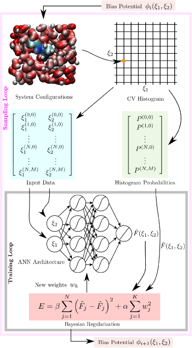
Figure 1: Schematic of the ANN adaptive biasing method. Hits along the collective variable(s) are recorded onto a histogram during the simulation. The discrete grid coordinates and corresponding reweighted normalized probabilities are used as the input and output training data respectively. An ANN architecture is chosen prior to runtime, and is trained iteratively using a Bayesian regularization procedure. The objective function chosen represents the sum squared error between the free energy estimate $\tilde{F}$ and ANN output $\hat{F}$. Hyperparameters $\alpha,\beta$ represent the relative penalties to the data and network weights respectively which are automatically adjusted during the optimization routine.

Figure 1 shows a schematic of the ANN sampling method. For a given CV $\xi$, the free energy along the CV is defined as

$$F(\xi)=-k_{\mathrm{B}}T\log{P(\xi)}.$$ (14)

Here $k_{\mathrm{B}}$ is Boltzmann’s constant, $T$ is temperature, and $P(\xi)$ is the probability distribution of the system along $\xi$, which the ANN method seeks to learn. Simulations proceed in stages or sweeps, indexed by $i$, where a bias, $\phi_{i}(\xi)$, is iteratively refined until it matches $-F(\xi)$. Typically, a simulation begins unbiased, though pre-trained networks may be loaded if available. The value of $\xi$ is recorded at each step into a sparse or dense histogram $H_{i}(\xi)$, depending on the CV dimensionality. Upon completion of a fixed number of steps, $N_{\mathrm{s}}$, this histogram is reweighted Torrie and Valleau (1977) according the bias applied during that sweep,

$$\tilde{H}_{i}(\xi)=H_{i}(\xi)e^{\frac{\phi_{i}(\xi)}{k_{\mathrm{B}}T}},$$ (15)

and subsequently added to a global partition function estimate,

$$Z_{i}(\xi)=\sum_{j\leq i}\tilde{H}_{j}(\xi).$$ (16)

Suitably scaled, this provides an estimator $\tilde{P}_{i}(\xi)$ with associated free energy

$$\tilde{F}_{i}(\xi)=-k_{\mathrm{B}}T\log\left[\tilde{P}_{i}(\xi)\right]$$ (17)

approximating the true FEL $F(\xi)$. As illustrated, the $\tilde{F}_{i}(\xi)$ serve as a training set for the ANN, using the discrete CV coordinates as input data. As a result, there are $N=\prod_{i=1}^{N_{CV}}M_{i}$ observations where $M_{i}$ is the number of bins along each CV $i$, and $N_{CV}$ is the total number of CVs. Henceforth, we will use a compact notation to denote the ANN architecture, with $\{5,2\}$ indicating a neural network with two hidden layers containing 5 and 2 neurons respectively. The output layer contains a single neuron defining a function $\hat{F}_{i}(\xi)$ comprising a best representation of the estimated free energy from the known data.

The bias for the initial sweep, $\phi_{0}(\xi)$ is defined at the outset. Subsequent sweeps utilize the ANN output via the equation $\phi_{i+1}(\xi)=-\hat{F}(\xi)$, where $\hat{F}$ denotes the optimized output of the neural network. By construction, this biasing function is continuous, differentiable, and free of ringing artifacts. Furthermore, one particular strength of this method is the capacity for a well–trained ANN to interpolate over the learned surface; each successive $\phi_{i}(\xi)$ yields a good estimate of the free energy even in poorly sampled regions, necessitating fewer samples in each histogram bin to obtain a high fidelity approximation of the FEL, as will be demonstrated below. The entire process is then iterated until the output layer $\hat{F}(\xi)$ achieves a measure of convergence to the true FEL $F(\xi)$.

III Results

III.1 One dimensional FEL

We first illustrate the robustness of the ANN method by studying a synthetic one dimensional Monte Carlo FEL composed of 50 Gaussians. The rugged landscape is meant to represent that of a glassy system or protein folding funnel; this exact surface was utilized as a benchmark for GFS Whitmer et al. (2015). Figure 2(a) shows the evolution of the ANN bias as a function of MC sweep $t$, where a sweep consists of $10^{5}$ moves. Utilizing a $\{40\}$ network, the analytical result is matched impressively within 40 sweeps ($4\times 10^{6}$ total MC moves). This highlights how even a parsimonious ANN is capable of capturing rugged topographies.

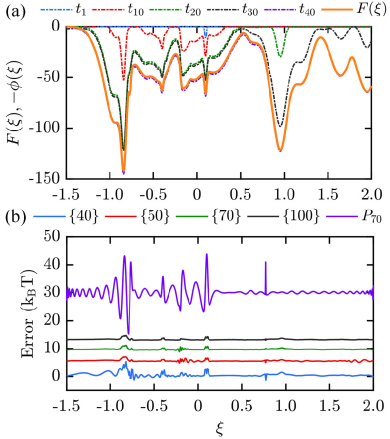
Figure 2: (a) Evolution of negative bias over time using a $\{40\}$ network on a benchmark rugged free energy landscape. The resolved bias converges to the $-F(\xi)$ smoothly over time with no apparent edge effects or oscillations in regions of steep derivatives. An analysis of the bias error (b) for different network sizes shows very good representation. There is a significant drop in error between $40$ and $50$ neurons after which the error signature stabilizes as a consequence of regularization. For comparison is a projection of the true surface onto an order $70$ Legendre polynomial which represents an ideal result for methods employing polynomial basis sets. Values have been shifted along the y–axis for clarity.

Further investigation into the effect of network size on the accuracy of the bias yields interesting results. Figure 2(b) shows the difference in $\phi(\xi)$ and $F(\xi)$ for network sizes from $\{40\}$ to $\{100\}$. While the smallest network does not exceed $5k_{\mathrm{B}}T$ in error, significant improvement is evident upon increasing the network size to $\{50\}$. Beyond this, error does not decrease significantly upon further refinement, indicating that Bayesian regularization converges to an effective number of parameters, demonstrating good generalization and lack of overfitting. Also plotted is a projection of the FEL onto a $70$ degree Legendre polynomial, which represents an idealized result of basis expansion methods Whitmer et al. (2014); Valsson and Parrinello (2014); Whitmer et al. (2015). There are clear minor oscillations across the entire interval and more pronounced ones in regions of sharp derivatives. Edge effects are also present with a substantial amount of error introduced at the right boundary. Remarkably, the ANN is capable of yielding a more accurate result using many fewer functions, while presenting no appreciable ringing.

Many free energy landscapes for meaningful systems are considerably smoother than this one-dimensional example. However, since adaptive sampling methods are iterative, initial estimates of even smooth surfaces are often noisy and sharply varying. This presents a challenge for basis expansion methods as one must use a large enough basis to drive the system out of metastable states yet one small enough that early sampling noise is effectively smoothed by low frequency truncation. Practically, the FEL can be recovered from a reweighted histogram which affords some flexibility in basis size, but the issue remains that enough terms must be retained to adapt to any features of significant size. The resulting emergence of oscillation artifacts greater than a few $k_{\mathrm{B}}T$ can unfortunately introduce significant sampling issues.

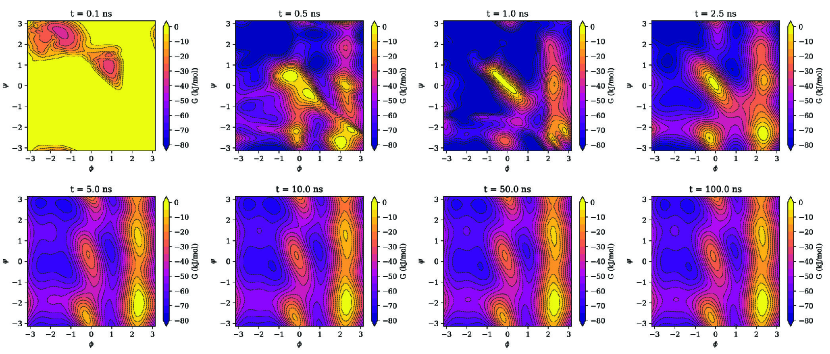
Figure 3: Snapshots of the estimated free energy landscape as a function of the Ramachandran angles for alanine dipeptide in water at $298.15$ K using ANN sampling on a $60\times 60$ grid. ANN sampling rapidly resolves the free energy landscape. Much of the speed of ANN sampling derives from its ability to smooth out statistical noise using the Bayesian framework and interpolate well in under–sampled regions at early times. Distortions are rapidly refined as the bias drives sampling to those regions and a stable approximation is achieved at approximately $5\ \mathrm{ns}$, where it is only subject to statistical fluctuations.

III.2 Two dimensional FEL: Alanine dipeptide in water

As a more realistic example, we study the isomerization of alanine dipeptide (ADP) in water. This system is a good testbed for free energy methods, as it has a rich FEL with significant variation and has been thoroughly studied. It is important to note that the dynamics of ADP in water are significantly slower than in vacuum, and is reflected in the convergence times of the free energy surfaces. The two torsional angles $\phi$ and $\psi$ of the ADP molecule are the CVs, which approximate McCarty and Parrinello (2017); Ma and Dinner (2005), but are not precisely, the slow modes of the isomerization process. ADP simulations are carried out in the NPT ensemble with a timestep of 2 fs and hydrogen bond constraints using the LINCS algorithm. Long-range electrostatics are calculated with particle mesh Ewald on a grid spaced at 0.16 nm. A stochastic velocity rescaling thermostat is used with a time constant of 0.6 ps to maintain 298.15 K and a Parrinello-Rahman barostat with a time constant of 10 ps maintains a pressure of 1 bar. The system consists of a single ADP molecule and 878 water molecules described by the Amber99sb and TIP3P forcefields respectively. A modified version of SSAGES v0.7.5 compiled with Gromacs 2016.3 was used for all simulations.

A periodic grid containing $60\times 60$ points is used with the ANN having topology $\{10,6\}$ and a chosen sweep interval of $10$ ps. Figure 3 shows snapshots of the estimated FEL at various time intervals. At early times one can see how the ANN is able to interpolate poorly–sampled and entirely unsampled areas within the vicinity of the initial exploration. The ANN bias is quickly refined as data are collected in these regions. Statistical noise is smoothed via the Bayesian regularization which forces a smooth network response at early times by increasing weight decay. After only $2.5\ \mathrm{ns}$ the bias closely resembles the final FEL, with only minor distortion of features present at regions of low probability. It is clear that even with limited and noisy data the ANN is able to construct an idealized, smooth interpolation of the FEL. In fact, the unbiased histogram used to train the ANN remains noisy for a significant amount of time after the network has converged. This is in stark contrast to other methods which rely on the unbiased histogram to recover an accurate FEL where the bias potential is unable to capture the fine details of the surface.

We investigate the sensitivity of ANN sampling to hyperparameters by studying six additional combinations of network architectures and sweep intervals. The reference FEL is the final ANN state after $100$ ns of simulation from the previous example. The new systems were run on a $30\times 30$ histogram, unlike the reference, to examine the behavior of ANN sampling with less available data and subject to larger discretization. Figure 4 shows the root mean square error (RMSE) of the FELs over time for the various systems. Except for a single setup, all FELs converged to within a $k_{\mathrm{B}}T$ at about $2.5$ ns, and $1$ kJ/mol at $5$ ns. The remaining configuration eventually converges at approximately $12$ ns. This relatively slow convergence represents the limit of network size and sweep length; a $\{8,4\}$ network is just able to represent the FEL, but requires more frequent updates and training. For the larger $\{10,6\}$ and $\{12,8\}$ networks, the sweep length has minimal impact on performance. For the end user, any reasonable choice of sweep length and a network of sufficient size should provide near optimal performance for new systems, eliminating the need for pilot simulations and significant prior experience.

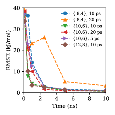
Figure 4: Free energy landscape root mean squared error (RMSE) for alanine dipeptide using various ANN architectures and sweep lengths as a function of time. The RMSE is computed relative to a reference FEL obtained from a $100$ ns simulation. With the exception of the small $\{8,4\}$ network with a large sweep, all other systems quickly converge to within $1k_{\mathrm{B}}T$ at $2.5$ ns, and within $1$ kJ/mol at $5$ ns. This demonstrates that beyond a minimum network size and sweep, the performance of ANN sampling is insensitive to a broad change of user-specified parameters.

III.3 Three dimensional FEL: Rouse modes of a Gaussian chain

We compute the three–dimensional dense free energy landscape of the three longest wavelength Rouse modes Rubinstein and Colby (2003) for a 21 bead Gaussian chain. This unconventional CV is useful in understanding the conformational dynamics of polymer chains, and represents a dense multi-variable FES which requires extensive visitation to resolve. The chosen system allows us to test the adaptability of ANN sampling to higher dimensions and compare the estimated FEL to analytical results for each Rouse mode $X_{i}$ by integrating over the others. The system was modeled using non-interacting beads connected via harmonic springs with bond coefficients of unity in reduced units. A Langevin thermostat was used to maintain a reduced temperature of $2/3$ integrated using the velocity-Verlet integrator with a timestep of $0.005$. A modified version of SSAGES v0.7.5 compiled with LAMMPS 30Jul2016 was used for the simulation.

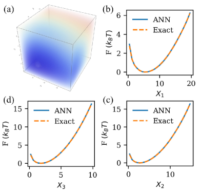
Figure 5: Dense three dimensional Rouse mode ($X_{i}$) free energy landscape for a 21 bead Gaussian chain. The 3D volume free energy (a) can be integrated along two chosen axes to yield the one–dimensional Rouse mode free energies. Comparison with analytical theory for (b) $X_{1}$, (c) $X_{2}$, and (d) $X_{3}$ show near exact agreement. This example demonstrates that ANN sampling should be useful in sampling correlated CVs in dense high dimensional spaces.

A $\{12,10\}$ network with a $N=25^{3}$ grid is used to converge the FEL. Figure 5 shows a volume rendering of the final FEL and the three integrated Rouse modes compared to theoretical prediction. The near exact agreement provides an objective measure of the accuracy of ANN sampling. Additionally, the number of hidden layers required to represent the FEL does not necessarily increase with the number of dimensions. Introducing a second hidden layer when going from a single to two or more dimensions is necessary to efficiently represent multidimensional surfaces, but a further increase is not strictly required. This is because the level set of neuron is a hyperplane and only upon composition (via the addition of another hidden layer) is multidimensional nonlinearity naturally representable.

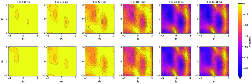
Figure 6: Evolution of 4D free energy estimate for alanine tripeptide in vacuum shown as two-dimensional Ramachandran plot projections. The top and bottom rows are the first and second $\psi$-$\phi$ pairs respectively. By $5$ ns, the bias has built up in the low-lying metastable configurations allowing for efficient diffusion of all CVs (cf. Fig. 7). The remaining time is spent resolving regions of extremely low probability which converges at approximately $20$ ns.

III.4 Four dimensional FEL: Alanine tripeptide in vacuum

In our final example we compute the free energy landscape of alanine tripeptide (Ace-Ala-Ala-Nme) in vacuum using all four backbone dihedrals as collective variables. This example was previously studied by Stecher et al.Stecher et al. (2014) using the CHARMM22 forcefield and Gaussian process regression (GPR). Here we use Amber99sb, hydrogen bond constraints, and a 2 fs timestep at $298.15$ K. Electrostatic interactions were handled using particle mesh Ewald and temperature was maintained using the stochastic velocity rescale thermostat. As with the previous examples, a modified version of SSAGES v0.7.5 was used compiled with Gromacs 2016.3.

We use a $\{24,20\}$ network with a $N=20^{4}$ grid and a sweep length of $20$ ps. As with the previous example, there is no need to introduce a third hidden layer. Figure 6 shows the evolution of the 4D free energy estimate projected onto two Ramachandran plots. ANN sampling rapidly builds up bias in the prominent free energy basins of the tripeptide, uncovering essential free energy basins and their structure within 5 ns of simulation time. This is allows the CVs to begin diffusing across these basins within a few nanoseconds, as shown in Figure 7. The remaining time is spent resolving regions of low probability, with a relative free energy as high as $90$ kJ/mol. Convergence is achieved at approximately $20$ nanoseconds with a reference FEL at a much later $60$ ns showing no appreciable change.

In Ref. Stecher et al. (2014), the 4D FEL of alanine tripeptide is reconstructed using GPR from an increasing number of short $500$ picosecond simulation windows. Qualitative agreement with a reference simulation is achieved after a total aggregate simulation time of $1.3$ microseconds. While a direct comparison is not possible, we find that the $20$ nanoseconds required to resolve the 4D FEL with ANN sampling to be remarkable. For high dimensional systems this corresponds to a substantial improvement in efficiency, where traditional methods can be prohibitively expensive. The results presented here from a single simulation, although ANN sampling is also trivially parallelizable. Our software implementation already contains support multiple walkers. Similar to GPR, this would allow multiple independent simulations to contribute to the same FEL, taking advantage of modern parallel architectures.

There are some additional important considerations for high dimensional CVs. As can be seen from our examples, we decrease the number of grid points per dimension as the system dimensionality increases. The simple reason for this is the curse of dimensionality: for a fixed point density, the training data size increases exponentially with increasing dimension. Furthermore, Bayesian regularization requires the calculation and storage of the Jacobian which scales as $\mathcal{O}(N^{2})$, and requires the inversion of the approximate Hessian. In an effort to minimize training time, we investigate the effect of limiting the maximum number of training iterations on the performance of ANN sampling.

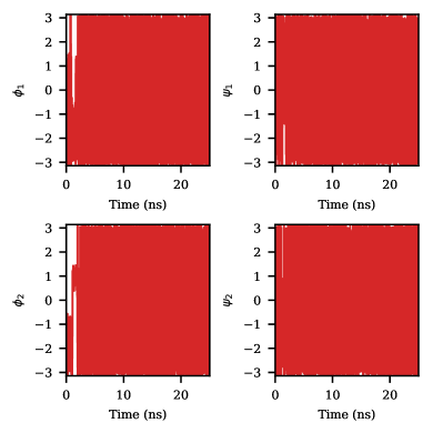
Figure 7: Time evolution of the four backbone dihedrals of alanine tripeptide which are used as collective variables with ANN sampling. $\phi_{1}$ and $\phi_{2}$ represent the slow modes of the peptide which are initially confined to metastable configurations. As bias accumulates each individual coordinate exhibits free diffusion across the metastable states; this occurs at approximately $3$ nanoseconds.

The results presented above were obtained using a maximum number of $10$ iterations per sweep. While this seems to be unreasonably small, it performs very well as shown. The reason for this is that in ANN sampling, the network weights are carried over each training cycle. This can be seen as a form of pre-training, where the network only requires a minimal amount of fine-tuning to adapt to new data. We also carried out the simulations using $20$, $50$, and $100$ maximum iterations and found little difference in performance, and due to the fewer iterations incurred much less overhead. These limitations are a result of targeting a uniform probability distribution in the collective variables. Targeting a well-tempered distribution or implementing a maximum fill-level on the free energy can be complimented with a sparse grid, since only regions of CV space accessible within a desired cutoff will be accessible. This sort of approach is often desirable and will scale better to even higher dimensions. We see this as an area of future research.

IV Discussion and Conclusions

We have presented a novel advanced sampling algorithm utilizing artificial neural networks to learn free energy landscapes. The ability of ANNs to act as universal approximators enables the method to resolve topologically complex FELs without presenting numerical artifacts typical of other methods which rely on basis sets. Bayesian regularization allows the entire set of training data to be used, prevents overfitting and eliminates the need for any learning parameters to be specified. This and other robust features result in a method which is exceptionally swift and accurate at obtaining FELs.

As ANN sampling superficially resembles the recently proposed NN2B method Galvelis and Sugita (2017), some remarks on their similarities and differences should be made. Though it also uses neural networks to estimate free energies, it differs significantly from out method beyond that. NN2B requires the specification of a large number of parameters, requiring significant knowledge of CV correlation times and sampling density, and it is not clear how they influence convergence. Our use of a discretized global partition function estimate retains information on all CV states sampled over the course of a simulation, while NN2B requires a judicious choice of the degree of subsampling from prior sweeps. The use of standard neural networks and their density estimation procedure necessitates significantly larger architectures and sampling intervals to represent a given free energy landscape. It also means that some of the valuable data must be used for validation to avoid overfitting.

The consequences of this are reflected in their study of alanine dipeptide in vacuum. Training times for each sweep are reported to range from 10 to 30 minutes depending on the size of the network. Furthermore, it requires 50 nanoseconds to converge the two dimensional FEL for ADP in vacuum. This is considerably longer than the typical 2 ns using standard metadynamics. In comparison, our method requires seconds to train the 2D FEL and a minute for higher dimensions in the early stages; as the approximate FES becomes smoother, the training time decreases considerably due to regularization. Both the lengthy training times and slow convergence render NN2B impractical for most applications. We do however see merit in using nearest neighbor density estimators in place of sparse histograms, and anticipate that this approach can be integrated within our proposed method.

The considerable advantages we have demonstrated biasing with ANN networks position this as an ideal method for the study of computationally expensive systems where sampling is limited. In particular, both first–principles MD and large biomolecule simulations are prime candidates for ANN sampling, where all but the most trivial of examples become intractable due to the typical time scales required to obtain free energy estimates. The significant speed improvements in sampling afforded by this method also open the door to the use of accelerated free-energy calculations for high throughput computational screening of material properties (see, e.g. Wilmer et al., 2012). The ANN framework also makes it possible to initialize simulations with pre–trained networks, a technique commonly used in deep learning applications. Starting with a FEL from a classical simulation can considerably improve the convergence of a first–principles estimate, while a theoretical or coarse–grained model can inform the initial bias in a biomolecular simulation. ANN sampling is a promising new approach to advanced sampling which can help resolve complex free energy landscapes in less time than conventional approaches while overcoming many previous shortcomings.

V Data availability

All of the run files, data, and analysis scripts required to reproduce the results in this paper are freely accessible online at https://github.com/hsidky/ann_sampling. ANN sampling will be available in the next SSAGES release.

VI Acknowledgements

HS acknowledges support from the National Science Foundation Graduate Fellowship Program (NSF-GRFP). HS and JKW acknowledge computational resources at the Notre Dame Center for Research Computing (CRC). HS and JKW acknowledge Michael Webb (U. Chicago) for providing the analytical Rouse mode solutions. This project was supported by MICCoM, as part of the Computational Materials Sciences Program funded by the U.S. Department of Energy, Office of Science, Basic Energy Sciences, Materials Sciences and Engineering Division.

References

- Barducci et al. (2013) A. Barducci, M. Bonomi, M. K. Prakash, and M. Parrinello, Proceedings of the National Academy of Sciences 110, E4708 (2013).
- Joshi et al. (2014) A. A. Joshi, J. K. Whitmer, O. Guzmán, N. L. Abbott, and J. J. de Pablo, Soft matter 10, 882 (2014).
- Valsson et al. (2016) O. Valsson, P. Tiwary, and M. Parrinello, Annual Review of Physical Chemistry 67, 159 (2016).
- Laio and Parrinello (2002) A. Laio and M. Parrinello, Proceedings of the National Academy of Sciences of the United States of America 99, 12562 (2002).
- Barducci et al. (2008) A. Barducci, G. Bussi, and M. Parrinello, Physical Review Letters 100, 020603 (2008).
- Singh et al. (2011) S. Singh, C. cheng Chiu, and J. J. de Pablo, Journal of Statistical Physics 145, 932 (2011).
- Dama et al. (2014) J. F. Dama, G. Rotskoff, M. Parrinello, and G. A. Voth, Journal of Chemical Theory and Computation 10, 3626 (2014).
- Branduardi et al. (2012) D. Branduardi, G. Bussi, and M. Parrinello, Journal of Chemical Theory and Computation 8, 2247 (2012).
- McGovern and De Pablo (2013) M. McGovern and J. De Pablo, Journal of Chemical Physics 139, 084102 (2013).
- Mezei (1987) M. Mezei, Journal of Computational Physics 68, 237 (1987).
- Hooft et al. (1992) R. W. W. Hooft, B. P. van Eijck, and J. Kroon, The Journal of Chemical Physics 97, 6690 (1992).
- Bartels and Karplus (1997) C. Bartels and M. Karplus, Journal of Computational Chemistry 18, 1450 (1997).
- Bartels and Karplus (1998) C. Bartels and M. Karplus, The Journal of Physical Chemistry B 102, 865 (1998).
- Valsson and Parrinello (2014) O. Valsson and M. Parrinello, Physical Review Letters 113, 090601 (2014).
- Whitmer et al. (2014) J. K. Whitmer, C.-c. Chiu, A. A. Joshi, and J. J. de Pablo, Physical Review Letters 113, 190602 (2014).
- Whitmer et al. (2015) J. K. Whitmer, A. M. Fluitt, L. Antony, J. Qin, M. McGovern, and J. J. de Pablo, The Journal of Chemical Physics 143, 044101 (2015).
- Kincaid and Cheney (2009) D. Kincaid and W. Cheney, Numerical analysis: mathematics of scientific computing (American Mathematical Society, 2009).
- Darve and Pohorille (2001) E. Darve and A. Pohorille, Journal of Chemical Physics 115, 9169 (2001).
- Comer et al. (2015) J. Comer, J. C. Gumbart, J. Hénin, T. Lelievre, A. Pohorille, and C. Chipot, Journal of Physical Chemistry B 119, 1129 (2015).
- Fu et al. (2016) H. Fu, X. Shao, C. Chipot, and W. Cai, Journal of Chemical Theory and Computation 12, 3506 (2016).
- Demuth et al. (2014) H. B. Demuth, M. H. Beale, O. De Jess, and M. T. Hagan, Neural Network Design, 2nd ed. (Martin Hagan, USA, 2014).
- Gletsos et al. (2003) M. Gletsos, S. G. Mougiakakou, G. K. Matsopoulos, K. S. Nikita, A. S. Nikita, and D. Kelekis, IEEE transactions on information technology in biomedicine 7, 153 (2003).
- Pao (2007) H.-T. Pao, Energy Conversion and Management 48, 907 (2007).
- Behler and Parrinello (2007) J. Behler and M. Parrinello, Physical Review Letters 98, 146401 (2007).
- Khaliullin et al. (2010) R. Z. Khaliullin, H. Eshet, T. D. Kühne, J. Behler, and M. Parrinello, Phys. Rev. B 81, 100103 (2010).
- Ma and Dinner (2005) A. Ma and A. R. Dinner, The Journal of Physical Chemistry B 109, 6769 (2005).
- So and Karplus (1996) S.-S. So and M. Karplus, Journal of Medicinal Chemistry 39, 1521 (1996).
- Li et al. (2015) Z. Li, J. R. Kermode, and A. De Vita, Phys. Rev. Lett. 114, 096405 (2015).
- Kumar et al. (1992) S. Kumar, J. M. Rosenberg, D. Bouzida, R. H. Swendsen, and P. A. Kollman, Journal of Computational Chemistry 13, 1011 (1992).
- Stecher et al. (2014) T. Stecher, N. Bernstein, and G. Csányi, Journal of Chemical Theory and Computation 10, 4079 (2014).
- Galvelis and Sugita (2017) R. Galvelis and Y. Sugita, Journal of Chemical Theory and Computation 13, 2489 (2017).
- Schneider et al. (2017) E. Schneider, L. Dai, R. Q. Topper, C. Drechsel-Grau, and M. E. Tuckerman, Physical Review Letters 119, 150601 (2017).
- Hornik et al. (1989) K. Hornik, M. Stinchcombe, and H. White, Neural Networks 2, 359 (1989), arXiv:1011.1669v3 .
- MacKay (1992a) D. J. C. MacKay, Neural Computation 4, 448 (1992a).
- MacKay (1992b) D. J. C. MacKay, Neural Computation 4, 415 (1992b).
- Nocedal and Wright (2006) J. Nocedal and S. J. Wright, Numerical optimization (Springer, New York, NY, 2006).
- Torrie and Valleau (1977) G. M. Torrie and J. P. Valleau, Journal of Computational Physics 23, 187 (1977).
- McCarty and Parrinello (2017) J. McCarty and M. Parrinello, arXiv preprint arXiv:1703.08777 (2017).
- Rubinstein and Colby (2003) M. Rubinstein and R. H. Colby, Polymer physics (Oxford University Press, New York, 2003).
- Wilmer et al. (2012) C. E. Wilmer, M. Leaf, C. Y. Lee, O. K. Farha, B. G. Hauser, J. T. Hupp, and R. Q. Snurr, Nature Chemistry 4, 83 (2012).