Theoretical transmission spectra of exoplanet atmospheres with hydrocarbon haze: Effect of creation, growth, and settling of haze particles. I.
Model description and first results
Abstract
Recently, properties of exoplanet atmospheres have been constrained via multi-wavelength transit observation, which measures an apparent decrease in stellar brightness during planetary transit in front of its host star (called transit depth). Sets of transit depths so far measured at different wavelengths (called transmission spectra) are somewhat diverse: Some show steep spectral slope features in the visible, some contain featureless spectra in the near-infrared, some show distinct features from radiative absorption by gaseous species. These facts infer the existence of haze in the atmospheres especially of warm, relatively low-density super-Earths and mini-Neptunes. Previous studies that addressed theoretical modeling of transmission spectra of hydrogen-dominated atmospheres with haze used some assumed distribution and size of haze particles. In this study, we model the atmospheric chemistry, derive the spatial and size distributions of haze particles by simulating the creation, growth and settling of hydrocarbon haze particles directly, and develop transmission spectrum models of UV-irradiated, solar-abundance atmospheres of close-in warm ( 500 K) exoplanets. We find that the haze is distributed in the atmosphere much more broadly than previously assumed and consists of particles of various sizes. We also demonstrate that the observed diversity of transmission spectra can be explained by the difference in the production rate of haze monomers, which is related to the UV irradiation intensity from host stars.
=3 \fullcollaborationNameThe Friends of AASTeX Collaboration
1 Introduction
Composition of exoplanet atmospheres is often measured by transit observation (e.g., Seager & Deming, 2010). When transiting in front of its host star, a planet blocks a fraction of the incident stellar light. The amount of blocked light relative to the original stellar light is called the transit depth. Since a set of transit depths observed at different wavelengths (called transmission spectrum) depends on atmospheric constituents, one can infer the atmospheric composition via multi-wavelength transit observations.
Recently, thanks to advance in observational techniques, atmospheric characterization for relatively small planets has become possible via transit observations. Typical examples are GJ 1214b of mass 6.26 and radius 2.80 (Charbonneau et al., 2009; Anglada-Escudé et al., 2013), GJ 3470b of 13.73 and 3.88 (Biddle et al., 2014), and GJ 436b of 25.4 and 4.10 (Lanotte et al., 2014). Interestingly, transmission spectra of those planets observed so far cannot be explained only by absorption and scattering (i.e., extinction) of gaseous molecules in the atmospheres.
GJ 1214b is a super-Earth whose atmosphere has been probed most. Recent multi-wavelength transit observations show a relatively featureless or flat spectrum from the optical (e.g. Narita et al., 2013; Nascimbeni et al., 2015) to near-infrared (e.g. Kreidberg et al., 2014), although de Mooij et al. (2012) reported a tentative increase in the transit depth in the optical. This raises the possibility that particles such as clouds and hazes are present in the atmosphere, because those particles obscure molecular absorption features. (In this study, we refer to thermochemical condensates as “clouds” and photochemical products as “hazes”.) Also, its transmission spectrum in the near-infrared is too flat to be explained even by a CO2-dominated atmosphere (Kreidberg et al., 2014). GJ 436b is also reported as showing a featureless spectrum in the near-infrared by Knutson et al. (2014), suggesting the presence of a cloudy/hazy layer.
GJ 3470b is reported to show a bit more complicated spectrum, which includes a steep spectral slope111The steep slope in the optical is sometimes referred to as the Rayleigh scattering slope in the literature. However, one can never conclude that the slope is due to Rayleigh scattering from an observed spectral slope alone (see Heng, 2016). in the optical (Fukui et al., 2013; Nascimbeni et al., 2013; Biddle et al., 2014; Dragomir et al., 2015; Awiphan et al., 2016) and is relatively featureless or flat in the near-infrared (Crossfield et al., 2013; Ehrenreich et al., 2014). A modest amount of cloud/haze particles, if present, tend to steepen the spectral slope in the optical (Lecavelier Des Etangs et al., 2008), while a thick cloud/haze obscures molecular and atomic absorption features, flattening the spectrum. Though the number of samples is still small, cloud/haze may be commonly present and bring about a diversity of spectra (Sing et al., 2016). Stevenson (2016) and Heng (2016) explored this diversity by quantifying the degree of cloudiness in atmospheres of transiting exoplanets from their spectra. Both two studies reported the trend that cooler planets were more likely to have cloudy/hazy atmospheres.
As a candidate for the cloud/haze, we consider hydrocarbon haze in this study for the reason below, while some other constituents are assumed in previous studies. The above three exoplanets are close-in super-Earths/mini-Neptunes orbiting M stars. Their atmospheric temperatures are typically 500 to 1000 K. Also, those close-in planets are exposed to intense UV radiation from their host stars. In such warm, highly-UV irradiated environments, hydrocarbon hazes are formed easily through photochemical reactions triggered by photo-dissociation of methane, provided the atmospheres are reducing enough that rather than CO dominates the atmospheric carbon chemistry (e.g. Yung et al., 1984). Note that a great number of exoplanets in the similar environments will be detected in near future, because MK dwarfs are most abundant in the solar neighborhood (e.g., Cantrell et al., 2013). Also, transit exoplanet surveys so far have detected many low-density low-mass exoplanets, which indicates that there are abundant low-mass exoplanets with relatively hydrogen-rich, reducing atmospheres (Fortney et al., 2007, and references therein).
Some studies so far addressed theoretical modeling of transmission spectra of hydrogen-rich atmospheres in such environments, considering the effect of haze in the atmosphere. Howe & Burrows (2012) is the first to quantify the effects of haze on transmission spectrum of GJ 1214b’s atmosphere. They assumed an atmospheric layer that contained haze particles such as tholin. The haze layer is characterized by four parameters, including single values of the number density and size of the haze particles and the pressures of the upper and lower edges of the haze layer. (They also considered the existence of clouds, below which transmitted light is cut off completely, regardless of wavelength.) Comparing their theoretical spectra with various haze/cloud properties and molecular compositions to the observed transmission spectrum of GJ 1214b, they demonstrated that a hydrogen-rich atmosphere with the haze layer could explain the observed transmission spectrum, provided appropriate sets of the haze parameters were chosen.
The same way for incorporating the effect of a haze layer was adopted by Ehrenreich et al. (2014), who modeled transmission spectra of GJ 3470b’s atmosphere and then compared them with the observed one, including their observations done with Hubble Space Telescope (HST). They found no solution that reproduced the observed steep spectral slope in the optical, simultaneously with the observed flat spectrum in the near-infrared. Instead, they concluded that both of the observed features in the visible and the near-infrared could be matched by a hydrogen-rich atmosphere covered with clouds, which they modeled in the same way as Howe & Burrows (2012).
In contrast to the above theoretical modelings that assume the altitude and thickness of the haze layer, Morley et al. (2013) tried to determine those properties by doing photochemical calculations. They derived numerically the vertical distributions of the photochemically-produced hydrocarbons, , , , and , which are precursors of haze particles. Assuming that haze particles formed from a given fraction of the precursors, which they regarded as a parameter (called the haze-forming efficiency), they determined the distribution of haze particles and then modeled the transmission spectrum of GJ 1214b’s atmosphere with assumed particle size and number density. (In their modeling, they used the opacity data of soot instead of those of tholin.) They found that the observed transmission spectra of GJ 1214b could be explained by the haze particles with the size of 0.01 to 0.25 m and the haze-forming efficiency of 1-5%, although there remained a possibility of clouds composed of KCl and ZnS.
The above studies certainly demonstrated that theoretical transmission spectra of hazy atmospheres matched the corresponding observations for appropriate choices of the haze parameters. However, they did not access the viability of those haze properties sufficiently from a physical point of view. In addition, transmission spectra so far observed seem to be diverse (Sing et al., 2016): In the visible, some show distinct spectral slope features, some may not. Also, some show molecular and atomic features, some are featureless. Again, although the previous studies found that choice of various haze parameters resulted in variation in transmission spectra, it remains to be clarified what yields such a variety of haze properties.
Of special interest in this study is the distribution of the size and number density of haze particles and its impacts on transmission spectra, which have not been investigated previously. Therefore we develop transmission spectrum models with detailed calculations of the creation, growth, and settling of hydrocarbon haze particles, assuming hydrogen-dominated atmospheres of close-in warm ( 1000 K) exoplanets. In this first paper, we focus on describing the methodology and demonstrating the sensitivity of transmission spectra to the production rate of haze monomers, which relates to the amount of UV irradiation from the host star. In our forthcoming papers, we make detailed investigation of the dependence of transmission spectra on model parameters, other than monomer production rate, such as atmospheric metallicity, C/O ratio, eddy diffusion coefficient, atmospheric temperature profile, and monomer size. Also, we explore in detail the composition of the atmospheres of known warm exoplanets by comparing the observed spectra with our theoretical ones, taking into account other possibilities of cloud/haze constituents.
The rest of this paper is organized as follows. In 2, we describe the assumptions, equations, and calculation methods for the size and number density distributions of haze particles and generating the transmission spectra. In 3, we investigate the vertical distribution of haze particles and its effects on the transmission spectra. Also, we investigate the dependence of the spectra on the production rate of haze monomers, which is related to UV irradiation intensity from the host star. In 4, to gain a deeper understanding of the effect of the haze particle distribution on transmission spectrum, we calculate the particle growth and transmission spectra with a characteristic-size approximation and then compare the results with those obtained in 3. Finally, we conclude this paper in 5.
2 Model and Method Description
As described in Introduction, we develop transmission spectrum models of warm transiting planets with hydrogen-rich atmospheres by incorporating the effects of the size and number density distributions of hydrocarbon haze that are determined through the production, growth, and settling processes of the particles. First, precursor molecules of haze particles (i.e., higher-order hydrocarbons, which we call haze precursors, hereafter) are created through photochemical reactions triggered by UV photodissociation of . Then, aggregation of the haze precursors results in haze particles of small size, which are called monomers. Note that the size of monomers in the atmosphere of Titan was reported as nm from observations (Tomasko et al., 2009). Those monomers diffuse and settle downward. Also, collisional growth of the haze particles takes place. Once the haze particles go down into hot, convective regions, they are likely to be thermodynamically broken and evaporated to be again, which can be diffused upward to be the source of haze precursors.
In this study, we first perform photochemical calculations to derive the vertical distribution of haze precursors in a similar way to Morley et al. (2013) ( 2.1). Then, using the obtained vertical profiles of the precursors, we calculate the growth and settling of haze particles in the atmosphere to derive the steady-state distributions of the size and number density of the haze particles ( 2.2). Finally, we calculate the extinction opacities of the gases and particles ( 2.3) and model transmission spectra of the atmospheres with obtained properties of haze ( 2.4).
Before explaining the details of the above three modules, we first describe the assumptions and treatments made in all the modules. We make an reasonable assumption that the atmosphere is in hydrostatic equilibrium and composed of ideal gases. While considering the altitude variation of gravity for hydrostatic structure, we neglect the effect of curvature, which would yield only a small difference compared to other large uncertainties in model parameters, and assume plane-parallel structure in the photochemical and particle growth calculations. In this paper, because our focus is on the effects of the size distribution of haze particles on transmission spectra, we assume, for simplicity, that the atmospheric structure is spherically symmetric. In reality, since close-in exoplanets tend to be tidally locked, the structure may be far from spherically symmetric. The details of this effect will be explored in our forthcoming papers.
2.1 Photochemical Model
Various photochemical models have been constructed for terrestrial and gaseous planets. Allen et al. (1981)’s model is for studying the vertical transport and photochemistry in the Earth’s mesosphere and lower thermosphere (50-120 km). Using their model, they derived the distributions of long-lived species and compared them with observations. Line et al. (2011) introduced their photochemical model to explore the chemistry of warm gaseous exoplanetary atmospheres for explaining the observed depletion of methane in the atmosphere of GJ 436b. Venot et al. (2012) released a large chemical network applying combustion models, which were validated over the temperature and pressure ranges relevant to hot Jupiter atmospheres. After that, they expanded their networks to hydrocarbons up to six-order (Venot et al., 2015). Hu et al. (2012) presented the photochemical model for terrestrial exoplanets applicable for all types of atmospheres, from reducing to oxidizing. They presented the results for three benchmark cases of atmospheric scenarios from reducing to oxidizing for terrestrial exoplanets. Tsai et al. (2017) presented an open-source photochemical model for hot exoplanetary atmospheres, VULCAN, which they validated by reproducing the results of Moses et al. (2011). In this study, we newly develop a photochemical model to derive the vertical distribution of haze precursors.
2.1.1 Model description
The one-dimensional continuity-transport equation that governs the change in the number density of species , , is written as (Yung & Demore, 1999)
| (1) |
where and are the time and the altitude, respectively, and are the production and loss rates of species due to photochemical and thermochemical reactions, respectively, and is the vertical transport flux of species . We assume that the vertical transport occurs by eddy diffusion and ignore molecular diffusion. The eddy diffusion flux is given by (Yung & Demore, 1999)
| (2) |
where is the eddy diffusion coefficient, is the total number density of the atmospheric gas molecules, and is the mixing ratio of species . Here, we have used the definition of atmospheric scale height and the ideal gas law.
We include the following 29 chemical species composed of the five elements, C, H, O, N, and He: , , , , , , , , , , , , , , , , , , , , , , , , , , , , and . These species are the ones considered in the photochemical models of Kopparapu et al. (2012), who studied the atmosphere of the hot Jupiter WASP-12b, except for and , which we do not consider. Since the main focus of this study is on calculating the size and spatial distributions of haze particles and evaluating their impacts on resultant transmission spectra, we simply assume that the haze precursors form from and , in the same way as Morley et al. (2013), and do not include higher-order hydrocarbons such as and . They showed that and are the most dominant hydrocarbons phtochemically produced in solar-abundance atmospheres with temperature of 500-1000 K, although there remains uncertainties for the treatment of higher-order hydrocarbons (see, e.g., Zahnle et al., 2016). Also, we do not consider sulphur compounds, because they are scarcely involved in reactions with hydrocarbons of interest here. As both the opacities of and are much smaller compared to those of and according to sulphur’s small elemental abundance, it is sure that they have little impact on the transmission spectrum. We do not consider Na and K because they condense as and clouds, respectively, and settle downward in the temperature range of interest ( 1000 K) (Morley et al., 2013).
We adopt 154 thermochemical reactions from the reaction list of Hu et al. (2012). All the thermochemical reactions and their rate coefficients are listed in Table 2. We have chosen the reactions that involve only some of the above 31 species, although the reaction list of Hu et al. (2012) contains more reactions. We also consider their reverse reactions using the method described in Visscher & Moses (2011). Thus, in total, we consider 308 thermochemical reactions. For the calculation of the Gibbs free energy of each species, which is needed to calculate the equilibrium constants (the ratios of forward to reverse reaction rate coefficients), we use the polynomial coefficients for calculating enthalpies of formation, entropies, and heat capacities from the Third Millennium Ideal Gas and Condensed Phase Thermochemical Database for Combustion 222http://garfield.chem.elte.hu/Burcat/burcat.html. Although some rate coefficients are invalid in the temperature range considered in this study, we use them outside their temperature range due to the lack of data and/or theory.
For photochemistry, we consider 16 reactions listed in Table 3. Likewise, all the reactions are extracted from the reaction list of Hu et al. (2012) if the reaction involves only some of the above 31 species. Photodissociation rate of species (i.e., the number of atoms or molecules dissociated per unit time) at altitude , , is written as
| (3) |
where is the wavelength, and are the dimensionless quantum yield of species , the absorption cross section (its physical dimension being area) of species , and is the actinic photon flux per unit area, unit time, and unit wavelength. The factor 1/2 is needed to account for diurnal variation (see Hu et al., 2012). The references from which we take the data of the quantum yields and absorption cross sections are tabulated in Table 4 and 3, respectively, most of which can be downloaded from the website of the MPI-Mainz UV/VIS Spectral Atlas of Gaseous Molecules of Atmospheric Interest333http://satellite.mpic.de/spectral_atlas. Temperature dependences of absorption cross sections are known for some of the species, but measured only in a temperature range between 200 and 300 K. Thus, following Hu et al. (2012), we calculate the absorption cross sections at 300 K by a linear interpolation with the use of the measured data and use them for temperatures higher than 300 K, namely , instead of extrapolating beyond 300 K. We consider the attenuation of the actinic flux as
| (4) |
where is the actinic flux at the top of the atmosphere at wavelength and is the cosine of the zenith angle of the star. is the optical depth defined by
| (5) |
where is the number of the species. We assume the zenith angle to be , as done in Hu et al. (2012). They found that the mean zenith angle differed depending on the optical depth of interest and concluded that the assumption of = -, which corresponded to = 0.1-1.0, was appropriate for the one-dimensional photochemical models.
For the boundary conditions, we set the diffusion flux as zero for all the species at the upper boundary, while we fix the volume mixing ratios of all the species at the thermochemical equilibrium values at the lower boundary. The exact conditions are, however, uncertain, so that previous studies chose different conditions at both boundaries. As for the upper boundary condition, while some studies set the diffusion flux equal to the assumed atmospheric escape flux (e.g., Hu et al., 2012), some studies set for all the species (e.g. Moses et al., 2011; Venot et al., 2012; Tsai et al., 2017). In this study, we choose the latter because the atmospheric escape rate is unknown for exoplanets. As for the lower boundary condition, photochemical modeling of terrestrial planet atmospheres often sets the flux of surface emission and/or deposition at the lower boundary (e.g., Hu et al., 2012). However, gas-rich planets, which we consider in this study, have no rigid surfaces. While some studies adopted zero flux (e.g., Moses et al., 2011; Venot et al., 2012; Tsai et al., 2017), we fix the volume mixing ratios of all the species at thermochemical equilibrium values in a similar way to, for example, Line et al. (2011) and Zahnle & Marley (2014). This is because the gases at deep levels would be in thermochemical equilibrium. While Moses et al. (2011) reported that they did not find any differences in the results between the two types of inner boundary condition, Tsai et al. (2017) found that only the minor ( ) molecules, CO and , deviated from their thermochemical equilibrium values at relatively cool (1000 K) lower boundary (1000 bar), but major molecules are in thermochemical equilibrium.
2.1.2 Calculation method
The calculation method we use in this study is basically the same as that used in previous works (e.g., Venot et al., 2012; Hu et al., 2012; Tsai et al., 2017). We discretize Eq. (1) as
| (6) |
where the subscript represents the physical quantities in the th layer and is the thickness of the th layer. We prepare layers with the same thickness and set the pressure at the mid-point altitude of the lowest layer as the lower boundary pressure. From Eq. (2), we approximate as (e.g., Venot et al., 2012; Hu et al., 2012; Tsai et al., 2017)
| (7) |
To obtain a steady-state solution, we solve Eq. (6) implicitly with the use of the solver DLSODES (Hindmarsh, 1982), which is suitable to solve stiff ODE systems such as chemical network calculations (e.g., Grassi et al., 2014). It is based on a backward differentiation formula (BDF), which is also called Gear’s method. The most suitable order is chosen within the solver. We set the maximum order allowed to be five. We adopt the values of relative (RTOL) and absolute (ATOL) tolerances as and , respectively; the value of ATOL differs from layer to layer.
The initial number densities of the species are set to their thermochemical equilibrium values, which we calculate in the following way. A system composed of gaseous species being considered, the Gibbs free energy of the system is minimized at equilibrium. The Gibbs free energy at fixed temperature , pressure , and composition is written as (Smith & Missen, 1982)
| (8) |
where and are the molar number and chemical potential of species , respectively, and . The chemical potential of an ideal gas is given by (Smith & Missen, 1982)
| (9) |
Here is the standard chemical potential that is a function of only, is the partial pressure of gaseous species , is the reference pressure, and is the molar gas constant. If a collection of species in the system is given, theoretically permissible chemical reactions can be derived from the law of conservation of mass:
| (10) |
where is the number of the th element contained in species and is the total number of moles of the th element. The composition that gives the minimum value of the Gibbs free energy is searched for to determine the equilibrium values of the mole fractions of the elements in the system. We assume vertically constant elemental abundance ratios and use the same Gibbs free energy data as that we use for calculation of reverse rate coefficients.
We time-integrate Eq. (6) until the system becomes in a steady state. We adopt the criteria of convergence such that all the species of vary in mixing ratio by less than 1% in all the layers. The integration is done over a period longer than the eddy diffusion timescale, which we assume as the maximum value of among all the layers at the initial condition. Here, is the atmospheric scale height for layer . The time step is self-adjusted within the solver so that the estimated local error in is not larger by an order of magnitude than that of ( ). At each time after calling the solver, for the atmosphere to be in hydrostatic equilibrium and the total mixing ratio to be unity, we set the output negative number densities to be zero, renormalize the volume mixing ratio of each species, recalculate the total number density at each layer assuming hydrostatic equilibrium, and calculate the number density of each species at each layer. Note that the output negative number densities are not larger by an order of magnitude than EWT.
We compare our photochemical model with the previous thermochemical models for the atmospheres of HD 189733b and HD 209458b presented by Tsai et al. (2017) in APPENDIX A and the photochemical models for the WASP-12b’s atmosphere presented by Kopparapu et al. (2012) in APPENDIX B. We have confirmed that the abundances of most of the species match those of the previous works within one order of magnitude and the profiles of the molecules are similar except for absolute value. And the differences in abundances for some molecules would not affect our results regarding haze distributions and transmission spectra. We have also confirmed the major trend found in those for GJ 1214b’s atmosphere (Miller-Ricci Kempton et al., 2012; Morley et al., 2013) and other low temperature ( K) atmospheres (Moses et al., 2013; Venot et al., 2014).
2.2 Particle Growth Model
We simulate the growth and settling of hydrocarbon haze particles after the production of monomers in the upper atmosphere and determine their steady-state distribution. We assume that monomers form in situ from the precursor molecules of haze particles. We assume and as the precursor molecules. While higher-order hydrocarbons may have to be also included as the precursors, previous studies (e.g., Morley et al., 2013) showed that and are the most dominant hydrocarbons photochemically produced in solar abundance atmospheres with temperature of 500-1000 K, as mentioned in § 2.1.
2.2.1 Model description
We follow the classical formalism for cloud particle growth (see Jacobson, 2005), which has also been used to simulate haze particle growth in Titan’s atmosphere (e.g., Toon et al., 1980, 1992). Note that the same formalism has been also used for dust particle growth in the field of planet formation (see, e.g., Armitage, 2010). Also, as for dust particle growth for brown dwarf atmospheres, there is a series of work (Woitke & Helling, 2003, 2004; Helling & Woitke, 2006), which is different from ours in the point that they considered particle growth due to chemical surface reactions but did not consider the growth due to coagulation.
Adopting a discrete volume grid, one can write the one-dimensional continuity-transport equation for the number density of particles with volume , , as (e.g. Lavvas et al., 2010)
| (11) | |||||
where the subscript denotes the volume grid, is the coagulation kernel between two particles with volumes and , and is the total number of volume bins used in the calculation. The first and second terms on the right-hand side describe the production and loss of the particles of volume (hereafter, the th particles, for simplicity) due to the coagulation. is the vertical transport flux and is the photochemical production rate of the th particles, which takes a non-zero value only for , namely monomers.
Assuming that the vertical transport occurs by sedimentation and eddy diffusion, one can write as (e.g. Lavvas et al., 2010)
| (12) |
where is the sedimentation velocity of the th particles written as (e.g. Lavvas et al., 2010)
| (13) |
Here, is the radius of the th particle, is the particle internal density, and is the local gravitational acceleration. is the dynamic viscosity defined as
| (14) |
where is the mass density of the gas, is the thermal velocity of the gaseous molecules defined as
| (15) |
with the Boltzmann constant , and the temperature , and the mean mass of gaseous molecules . is the atmospheric mean free path defined as
| (16) |
with the pressure and the diameter of the gas molecule . Because is the most abundant gas species in the atmosphere of interest in this study, we use the diameter of for the value of , taken from CRC Handbook of CHEMISTRY and PHYSICS (Haynes, 2012). is the Cunningham slip-flow correction factor given by (Davies, 1945)
| (17) |
where is the Knusden number defined as .
As for coagulation, we consider two rate-controlling processes which include the Brownian diffusion and gravitational collection. The latter is the collisional process that occurs as a result of difference in sedimentation velocity between different size particles. The total kernel is assumed to be the sum of the two kernels, namely
| (18) |
The Brownian collision kernel for the th and th particles, , can be written as (Jacobson, 2005)
| (19) |
with
| (20) |
and are the diffusion coefficient and thermal velocity for the th particle, respectively. These parameters are given as
| (21) |
and
| (22) |
with the particle mass . is the particle’s mean free path written as
| (23) |
The gravitational collection kernel for the th and th particles, , can be written as (Jacobson, 2005)
| (24) |
where is a collision efficiency given by
| (25) |
| (28) |
| (29) |
Here, is the Reynolds number written as
| (30) |
with the kinematic viscosity
| (31) |
and is the Stokes number written as
| (32) |
When we simulate the particle growth with the discretized size distribution, we face the problem that the coagulation between the th and th particles () produces particles of an intermediate volume,
| (33) |
To satisfy the conservations of the mass and the particle numbers at the same time, we partition this intermediate-volume particle into the two volume bins, and (), with fractions and , respectively. Unless is the largest volume bin, these fractions can be written as
| (34) |
and
| (35) |
If is the largest volume bin, we cannot partition the intermediate particle but just put it into the largest volume bin , although the mass conservation is not satisfied. We specify the volume ratio of two adjacent bins in 2.5.
2.2.2 Monomer production rate
As described above, we assume that monomers are formed in situ from the precursor molecules and . Thus, we calculate the vertical profile of the mass production rate of monomers according to the distribution of the two molecules. We consider that the mass production rate of monomers, which means the total mass of monomers produced per unit volume per unit time, at altitude is given by
| (36) |
where and are the volume mixing ratios of HCN and , respectively, and is the total mass production rate of monomers throughout the atmosphere and its physical unit is mass/area/time.
We assume that is proportional to the incident stellar Lyman-alpha (Ly) flux at the planet’s orbital distance, , because monomer production is relevant to UV photodissociation. Thus, we assume the photochemistry of monomer formation to be driven entirely by . For the reference, we use the observed values of the incident solar Ly flux, , and mass production rate, , in the present Titan’s atmosphere; Nnamely,
| (37) |
This is a simpler version of Eq. (8) of Trainer et al. (2006), which they derived empirically. Although both linear and quadratic dependences of on are proposed, there is still room for discussion to determine which relationship is appropriate (Trainer et al., 2006). The linear relationship would be valid when haze monomers are produced predominantly by photodissociation of hydrocarbon intermediate molecules, which is the product of photodissociation of , while the quadratic relationship would be valid when haze monomers are produced mainly by thermochemical reactions between multiple intermediates (see Trainer et al. (2006) for details). Because the relationship is totally uncertain for exoplanet atmospheres, we have adopted the linear relationship for simplicity, and added a numerical parameter in the above equation. We adopt g for , since microphysical models, photochemical models, and laboratory simulations all imply that the production rate of the monomers on Titan is in the range between and g (McKay et al., 2001). Also, we use photons for (Trainer et al., 2006). When we vary , we also vary the intensities of the actinic flux at all the wavelengths according to (i.e., the Ly intensity).
Finally, the boundary conditions for Eq. (11) are given as follows. As the lower boundary conditions, we consider that all the particles are lost with the larger of the sedimentation velocity and the downward velocity imposed by the atmospheric mixing, following Lavvas et al. (2010). As the upper boundary conditions, we set zero fluxes for all the particle sizes.
2.2.3 Calculation method
We divide the atmosphere into layers with the same thickness and discretize Eq. (11) as
| (38) | |||||
where the subscript represents the physical quantities in the th layer. We set the pressure at the mid-point altitude of the lowest layer as the lower boundary pressure. For Eq. (12), we use the upwind difference scheme instead of the central difference scheme for the calculation of sedimentation flux, because of numerical stability, and approximate as
To obtain a steady-state solution, we solve the continuity Eq. (38) implicitly with the same solver DLSODES (Hindmarsh, 1982) that we use in the photochemical calculations ( 2.1). We adopt the values of relative (RTOL) and absolute (ATOL) tolerances as and , respectively. The initial number densities of all the sizes are set to zero. We adopt the criteria of convergence such that the volume-averaged sizes of particles in all the layers, which we calculate as
| (40) |
are different by less than 1%.
2.3 Opacity
2.3.1 Haze particles
We calculate the extinction cross sections of haze particles based on the Mie theory (Mie, 1908). In the limit where the particle radius, , is large compared to the radiation wavelength, , the Mie theory agrees with geometric optics. On the other hand, the Mie theory reduces to the Rayleigh theory in the limit of .
From the Mie theory, the extinction cross section of a homogeneous spherical particle of radius , , can be written as (Bohren & Huffman, 2004)
| (41) |
where Re denotes the real part. Here, is the size parameter defined as
| (42) |
Coefficients and are calculated as
| (43) |
and
| (44) |
where is the ratio of the complex refractive indices of the particle to the surrounding atmosphere. and are the so-called Ricatti-Bessel functions and the prime indicates differentiation with respect to the argument in parentheses.
We use the bhmie code (Bohren & Huffman, 2004) to calculate Eqs. (41)-(44). Complex refractive indices of haze are taken from Khare et al. (1984), which reports laboratory experiment results for production of tholin hazes in a simulated Titan’s atmosphere (0.9 /0.1 gas mixture at 0.2 mb).
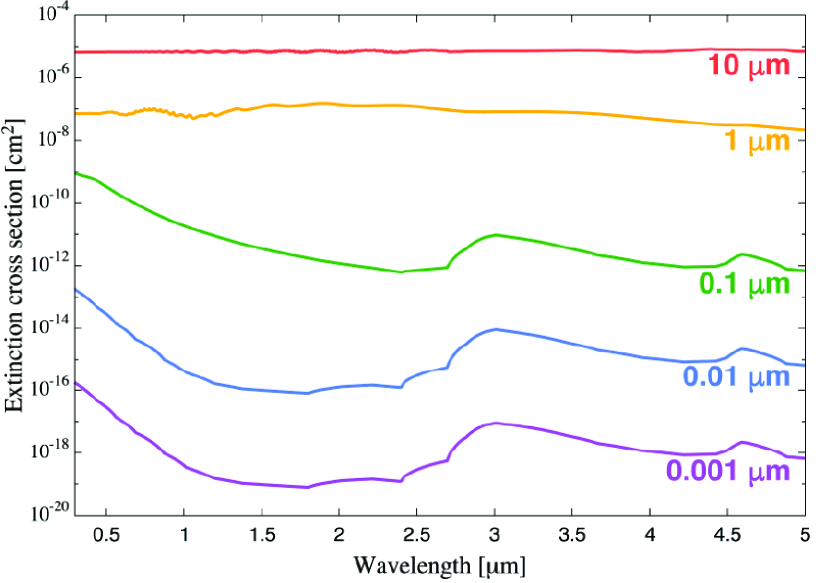
In Figure 1, we show the extinction cross sections of the haze particles of five different particle sizes, namely, 0.001 , 0.01 , 0.1 , 1 , and 10 . When the particle size is sufficiently small relative to the wavelength, the scattering is approximated by the Rayleigh scattering. More specifically, the cross sections for 0.001 , 0.01 , and 0.1 show the behavior due to the Rayleigh scattering in the visible wavelength region; namely, . Also, the dependence on the particle radius is such that (e.g., Petty, 2006). In contrast, for larger particles of 1 m and 10 m, no such feature is found, and the cross sections are relatively independent of wavelength. Note that the bumps found around and come from the vibrational transitions of the C-H bond and CN bond of the tholin-like haze particles, respectively (Khare et al., 1984).
2.3.2 Gaseous species
For another source of radiative extinction in the atmosphere, we consider line absorption by , , , , , , , , , , and . We ignore the extinction by Na and K because they condense as and clouds, respectively, and settle downward in a temperature range of interest ( 1000 K) (Morley et al., 2013).
The extinction cross section of species , at wavenumber , , is written as
| (45) |
where is the line absorption cross section for the transition from lower state to upper state .
For briefly, we omit the subscript hereafter. The line absorption cross section, , is given as
| (46) |
where is the spectral line transition wavenumber, is the spectral line intensity, and is the line profile function. We calculate , using the line data from HITRAN2012 (Rothman et al., 2013). When summing the absorption cross section for each transition, we do not consider the cross sections whose spectral line intensities are less than because of the computational cost.
According to Sharp & Burrows (2007) and Rothman et al. (1998), the spectral line intensity at temperature , , is written as
| (48) | |||||
where is the statistical weight of the lower state , is the oscillator strength for the transition between the lower and upper states, and are the lower-state and upper-state energy, respectively, and is the total internal partition function at temperature . is the elementary charge, is the electron mass, and , , and are the Planck constant, the speed of light, and the Boltzmann constant, respectively. is the spectral line intensity at the reference temperature and written as
| (49) | |||||
The HITRAN2012 database provides the values of , , , and , where . We calculate with the total internal partition sums (TIPS) code (Fischer et al., 2003) in the HITRAN database. This code calculates for given temperature (the temperature range is 70-3000 K) and molecular species in the HITRAN database.
We consider the air-broadened pressure-shift in the following way. The shifted spectral line transition wavenumber can be written as
| (50) |
where is the air-broadened pressure shift, provided that the shift, , is small relative to . Here, is the reference pressure. The HITRAN2012 database provides the values of , which we use in calculating the line absorption cross sections.
As for line broadening, we consider pressure broadening and Doppler broadening. The line profile for pressure broadening is given by the Lorentz profile (Petty, 2006),
| (51) |
where is the line half width of the pressure broadening. On the other hand, the line profile for Doppler broadening is given by the Gaussian profile (Petty, 2006),
| (52) |
where is the line half width of the Doppler broadening.
To consider both line profiles, the convolution of the Lorentz and Gaussian profiles, which is called the Voigt profile, is used:
| (54) | |||||
| (55) |
where is called the Voigt function and defined as
| (56) |
For the calculation of the Voigt function, we use the polynomial expansion of this function (Kuntz, 1997; Ruyten, 2004). We adopt any cut-off in the line wings.
In the HITRAN2012 database, the line half width of the pressure broadening is calculated as
| (57) | |||||
where and are, respectively, the air-broadened halfwidth and the self-broadened halfwidth at half maximum (HWHM) at K and atm and is the partial pressure. The line half width of the Doppler broadening is given by
| (58) |
where is the mass of the molecule (Petty, 2006).
We also consider the Rayleigh scattering by those molecules except and the collision-induced absorption by - and -. We have confirmed that the Rayleigh scattering by OH is negligible for the total extinction by all the molecules because of its low abundance in the atmosphere. The Rayleigh scattering cross section is given by (Liou, 2002)
| (59) |
where is the polarizability. We use the value of the polarizability for each molecule from CRC Handbook of CHEMISTRY and PHYSICS (Haynes, 2012). The collision-induced absorption cross sections are taken from HITRAN2012 (Rothman et al., 2013).
2.4 Transmission Spectrum Model
We model transmission spectra following Brown (2001). The transit depth at wavelength , , can be defined as
| (60) |
Here, is the disk-integrated luminosity from the host star given by
| (61) |
where and are the stellar radius and flux, respectively, and is the impact parameter measured from the disk center. is the disk-integrated luminosity of the host star during transit. Here, we assume that the incident stellar light rays are parallel and thus is constant through the stellar disk, because the orbital distances of planets of interest are much larger (by a factor of 10-100) than the host star’s radius. With this assumption, is expressed as
| (62) |
where is the so-called chord optical depth defined by
| (63) |
Here, and are the extinction cross section and number density of species , is the number of species whose extinction is considered, and is the line element along the line of sight.
In this study, we assume that all the parts inside the sphere of radius are optically thick enough to block the incident stellar light completely. The radius may be defined as that of a solid surface or an optically thick cloud deck in the atmosphere, if present. However, some exoplanets may have no such well-defined boundary. Even if there is such a boundary, its radius is unknown in advance. According to our numerical results, is sufficiently larger than unity below the pressure level of 10 in the atmosphere considered in this study. Thus, we define as the radial distance from the planetary center at which the pressure is 10 bar.
2.5 Calculation Procedure and Model Parameters
Finally, we summarize the calculation procedure and the model parameters and their values that we use in our simulations.
First, we derive the vertical profiles of volume mixing ratios of the gaseous species, , from the photochemical calculations ( 2.1). Then, from the sum of and , which corresponds to the distribution of the haze precursors, we simulate the particle growth and calculate the number density distribution of each haze volume ( 2.2). After that, with the obtained size and number density distributions of haze particles and the vertical distribution of the gaseous species, we model transmission spectrum of the atmosphere ( 2.4) with calculations of opacities of gaseous species and haze particles ( 2.3). The opacity and transit depth is calculated every wavenumber grid with width of 0.1 .
In this study, we model the transmission spectra assuming the properties of the super-Earth GJ 1214b. Among super-Earths found so far, the atmosphere of GJ 1214b has been probed most by transit observations at multiple wavelengths. The model parameters and their values we use are listed in Table 1. We will explore dependence of results on model parameters other than monomer production rate such as metallicity, C/O ratio, eddy diffusion coefficient, atmospheric temperature profile, and monomer size in our forthcoming papers.
We adopt the value of the radius at the 1000-bar pressure level (simply called the 1000-bar radius, hereafter) as 2.07 , which is 74% of the planet radius reported by Anglada-Escudé et al. (2013); We have found that this value of the 1000-bar radius can roughly match the observed transit radii of GJ 1214b when we assume a clear solar composition atmosphere. Note that when we infer the molecular abundance from observational transmission spectrum, we suffer from degeneracy among the reference radius, 1000-bar radius, and inferred molecular abundance (see Heng & Kitzmann, 2017).
For the temperature-pressure profile, we use the analytical formula of Guillot (2010), because its smooth and simple function suits computationally-heavy photochemical calculations. With Eq. (29) of Guillot (2010), we calculate the temperature-pressure profile averaging over the whole planetary surface (i.e., in the equation). We choose the parameters, namely, the intrinsic temperature , equilibrium temperature , averaged opacity in the optical , and averaged opacity in the infrared , so as to match the temperature-pressure profile of GJ 1214b that Miller-Ricci & Fortney (2010) derived for a solar composition atmosphere under the assumption of efficient heat redistribution from the day and night sides. This yieds K, K, , and . We have confirmed that our profile agrees with that of Miller-Ricci & Fortney (2010) within 86 K for the grids we adopt. We adopt the value of eddy diffusion coefficient as . We will explore the sensitivity of transmission spectrum to eddy diffusion coefficient in our forthcoming papers. As for the elemental abundance ratios, we assume that of the solar system abundance, which we take from Table 2 of Lodders (2003), corresponding to C/O, O/H, and N/H of , , and , respectively.
As for the stellar spectrum used in the photochemical model, we use that of GJ 1214 constructed by the MUSCLES Treasury Survey (France et al., 2016; Youngblood et al., 2016; Loyd et al., 2016), the wavelength coverage of which is from 0.55 nm to 5500 nm. The spectrum for X-rays is constructed from Chandra/XMM-Newton and APEC models (Smith et al., 2001), that for EUV from empirical scaling relation based on Ly flux (Linsky et al., 2014), that for Ly from model fit to line wings (Youngblood et al., 2016), and that for visible–IR from synthetic photospheric spectra from PHOENIX atmosphere models (Husser et al., 2013). We use the version 1.1 of the panchromatic SED binned to a constant 1 Å resolution and downsampled in low signal-to-noise regions to avoid negative flux, the data of which is taken from the MUSCLES team’s website444https://archive.stsci.edu/prepds/muscles/. We adopt 1 angstrom as the spectral resolution we use. The Ly flux of GJ 1214, which is located at 14.6 pc far away from the Sun, was observed as erg at the Earth (Youngblood et al., 2016). From this value, we calculate the Ly flux at the planet’s orbit as photons using the value of GJ 1214b’s semi-major axis, 0.0148 AU (Anglada-Escudé et al., 2013), and the Ly wavelength of 121.6 nm. Note that when considering the effects of the mass production rate of haze monomers (i.e., the Ly flux), we vary the intensities of the actinic flux at all the wavelengths according to the Ly intensity.
As for the monomer radius , we adopt m. We prepare 40 volume bins, setting the volume ratio of two adjacent bins to be 3 (Lavvas et al., 2010), and cover from m (monomer size) to 1600 m. As for the value of haze particle internal density , we adopt g , which is adopted by most of the particle growth models for hydrocarbon hazes in Titan’s atmosphere (e.g. Toon et al., 1992; Lavvas et al., 2010).
In the photochemical calculations, the atmosphere is vertically divided into 165 layers with thickness of 45 km, placing the lower boundary pressure at 1000 bar. This thickness is sufficiently smaller relative even to the minimum atmospheric scale hight in the atmosphere, which is 177 km. In the case of the particle growth model, we consider the pressure range from 10 bar to bar with 200 same thickness layers.
Simplified version of our transmission spectrum models are used for WASP-80b in Fukui et al. (2014) and for HAT-P-14b in Fukui et al. (2016). In the spectrum models of Fukui et al. (2014), we ignored the photochemical reactions and regarded the particle size, particle number density, altitude and thickness of the haze layer as input parameters. In Fukui et al. (2016), we did not consider the effects of haze on the spectra.
| Parameter | Description | Value | Reference |
|---|---|---|---|
| Host star radius | 0.201 | Anglada-Escudé et al. (2013) | |
| Planet mass | Anglada-Escudé et al. (2013) | ||
| bar | 1000-bar radius | 2.07 | |
| Eddy diffusion coefficient | |||
| Monomer radius | m | ||
| Particle internal density | g | ||
| Ly flux at the planet’s orbit | photons | Youngblood et al. (2016) |
3 Results
In this section, we show results of our numerical simulations. First, we investigate the fiducial monomer production case (i.e., ) in § 3.1-3.3 and then explore the dependence on the monomer production rate by changing in § 3.4.
3.1 Photochemical Calculations
First we outline the photochemistry of the atmosphere. Although the results we show below are basically the same as those from the previous studies, we show them because they are helpful in interpreting our later results. We note that our photochemical models of GJ 1214b’s atmosphere are the first ones that use the observed GJ 1214’s UV spectrum (France et al., 2016; Youngblood et al., 2016; Loyd et al., 2016).
Figure 2 shows the calculated vertical distributions of gaseous species in the photochemical equilibrium state (solid lines). We also present the distributions obtained by thermochemical equilibrium calculations (dashed lines) that ignore photochemical processes and eddy diffusion. In the lower atmosphere ( bar), the eddy diffusion mixing, which tends to smooth out compositional gradients, is found to yield constant abundances of , , , , and CO equal to the lower boundary values. In the upper atmosphere ( bar), it turns out that many species (i.e., , , , , , , , , , , , , and ) that are quite rare in thermochemical equilibrium states are produced photochemically and H is the most abundant species. The H is known to act as a reactive radical in reducing atmospheres (Hu et al., 2012).
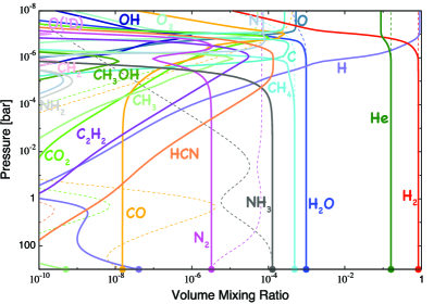
As for the haze precursors, HCN and , is always greater than . This means that in our simulations, the profile of the production rate of monomers is determined mainly by that of . The ratio is constant in the pressure range of bar to bar because HCN is the most stable N-bearing species in this range.
The details of the production and loss mechanisms of HCN and was discussed in Moses et al. (2011) for the cases of two hot Jupiters, HD 189733b and HD 209458b. Nevertheless, below, we also explore how the steady-state abundances of HCN and are maintained, since the atmospheric temperature considered in this study is lower than HD 189733b ( K) and HD 209458b ( K555http://www.openexoplanetcatalogue.com).
In Figure 3, we plot the distributions of the production and loss rates of HCN due to thermochemical and photochemical reactions, and transport by eddy diffusion for the steady-state distribution of HCN. In the pressure range of bar to bar, the steady-state is maintained almost by the production process via the thermochemical reaction,
and the loss process via photodissociation,
On the other hand, in the pressure range of bar to bar, the steady-state is maintained by a balance between the production process via the thermochemical reaction,
and the loss process via eddy diffusion transport to the upper atmosphere.
Figure 4 is the same as Fig. 3 but for . In the pressure range of bar to bar, the steady-state is determined by the production process via the thermochemical reaction,
and the loss process via photodissociation,
On the other hand, in the pressure range of bar to bar, the steady-state is determined by production process via the thermochemical reaction,
and the loss process, via photodissociation,
3.2 Particle Growth Calculations
The growth of haze particles occurs via competition among coagulation, sedimentation, and diffusion. Knowledge of the sedimentation velocity is therefore helpful in understanding the particle growth. Figure 5 shows the sedimentation velocity along pressure for five different particle radii, m, m, m, m, and m. Change of the trend found at bar for the 59 m particle and bar for the 1600 m particle, respectively, results from the transition from slip flow () to Stokes flow (). In the slip flow regime, the sedimentation velocity is proportional to the particle radius (see Eqs. (13) and (17)). On the other hand, in the Stokes flow regime, the sedimentation velocity is proportional to the square of the particle radius (see Eqs. (13) and (17)).
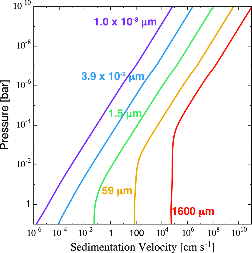
Figure 6 shows the vertical profiles of haze properties. Here, we define the surface average radius (yellow solid line) as
| (66) |
and the volume average radius (red solid line) by Eq. (40). If the two average sizes agree with each other at a certain altitude, the size distribution is unimodal at the altitude. The surface average number density (yellow dashed line) and the volume average number density (red dashed line) are calculated as
| (67) |
and
| (68) |
respectively. Also, the mass densities for all the size bins at each pressure level are plotted with the blue color contour and the vertical profile of the monomer mass production rate is plotted with the green solid line.
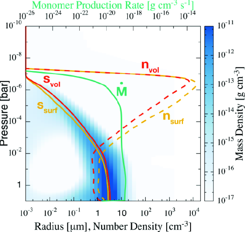
From Fig. 6, it is demonstrated that the average radii change dramatically with altitude. In the upper atmosphere, particles grow little because they settle faster than coagulational growth proceeds. The number densities become larger as altitude decreases (or the pressure increases) and they take the peak value at bar. Coagulational growth occurs significantly below this pressure level. As altitude decreases, the average radii increase from m to 2-3 m because of coagulational growth, and the number densities decrease by several orders of magnitude from the peak values. Again, change of the trend found at bar results from the transition from the slip flow to Stokes flow regimes. A significant increase in the sedimentation velocity due to the regime transition of drag force (see Fig. 5) inhibits the collision between particles.
The slight difference between and means that the haze contains different size particles at each altitude. The color contour indicates that particles in some narrow range of size are abundant at each altitude and the monomer size particles exist broadly below the level of bar because monomer production occurs in this region.
In Figure 7, we plot the distributions of number density of haze particles for all the size bins at seven different pressure levels, bar, bar, bar, bar, bar, 0.95 bar, and 10 bar. First it is found that the number density of monomer size, m, is the largest among all the sizes at all the pressure levels because of the large monomer production rate. At low pressures of bar, the coagulation due to brownian diffusion is the dominant process, whereas that due to gravitational collection hardly occurs. On the other hand, at high pressures of bar, both coagulation mechanisms contribute to the particle growth. The coagulation due to gravitational collection makes a second peak of number density for the pressure levels higher than bar, because it occurs in a runaway fashion much more rapidly compared to that due to brownian diffusion.
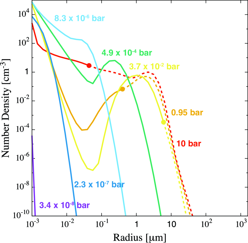
The change of size distribution can be understood as follows: The particles grow through the frequent collisions with the abundant small particles. The collision timescale between a large particle and monomer size particles can be written as , where is the number density of monomers, is the collision cross section of the large particle, and is the relative velocity between the particles. The relative velocity due to sedimentation is proportional to particle radius in the slip flow regime and in the Stokes flow regime (see Eqs. (13) and (17)), while the relative velocity due to brownian diffusion is proportional to (see Eq. (22)). Thus, (slip flow) and (Stokes flow) for gravitational collection, while for brownian diffusion. This means the particle growth is always a runaway process: The larger the particle, the faster the growth proceeds. Also, the gravitational collection is much faster than the brownian diffusion especially for large size particles. Therefore, from bar on, the second peak grows rapidly and a valley-shaped distribution develops (see yellow and orange lines), because gravitational collection contributes predominantly to the particle growth above this pressure.
At bar, however, the valley is found to disappear. This is because the drag law for the large particles shifts from the slip flow regime to the Stokes regime. In Fig 7, the Stokes regime is indicated by dashed lines, while the slip flow regime is indicated by solid lines; the transition points are marked by filled circles. Since the sedimentation velocity is so high in the Stokes regime (see Fig. 5) that the particles settle faster than they grow, the largest-size group ( 2 m) stops growing (see the orange lines). Then, small particles, which are still in the slip flow regime, grow and are catching up with the largest particles.
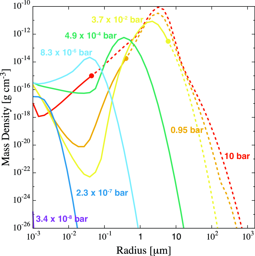
In Figure 8, we plot the distributions of mass density for all the size bins at the same set of seven different pressure levels as shown in Fig. 7. It can be noticed that there are dominant sizes that account for most of the total haze mass for all the seven pressure levels. And the dominant size becomes larger, as pressure increases, because of the coagulational growth.
3.3 Transmission Spectrum Models
Figure 9 shows the transmission spectrum models for the atmosphere with haze (green line) and without haze (black line). Also, the relative cross section of the planetary disk with radius corresponding to a certain pressure level, which is defined as
| (69) |
is presented by horizontal dotted lines from bar to bar for the atmosphere without haze. In equation (69), and are the radius at the pressure level and the stellar radius, respectively. Roughly at these pressure levels, there exist the molecules accountable for the spectral features. We have confirmed that the chord optical depth at the pressure that corresponds to the transit radius is between 0.1 and 1, depending on wavelength. Note that the transmission spectrum models are smoothed for clarity by averaging over the nearest 633 wavenumber points, namely 63.2 , for each point. We use the same smoothing method for the results of spectrum models hereafter.
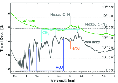
In the spectrum model for the atmosphere without haze (black line), several characteristic spectral features can be seen. For example, prominent features of are found around 0.7 m, 0.8 m, 0.9 m, 1.2 m, 1.3-1.6 m, 1.9 m, and 2.5-3.0 m, those of around 1.7 m, 2.2-2.4 m, and 3.3 m, and that of around 3.0 m. The Rayleigh scattering feature mainly due to can be seen in the optical wavelength region.
The spectrum for the atmosphere with haze (green line) is relatively featureless, compared to that for the atmosphere without haze (black line). This is because the haze particles in the upper atmosphere ( bar) makes the atmosphere optically thick and prevent the molecules in the lower atmosphere ( bar) from showing their absorption features. However, the small features of above bar can be seen at 2.2-2.4 m and 3.3 m because of their large extinction cross sections at these wavelengths. Also, the spectral features due to the C-H and CN bonds of the haze particles appear at 3.0 and 4.6 m, respectively.
In the wavelength region of 0.3-1 m (green line), the spectral slope due to Rayleigh scattering by small ( m) haze particles in the upper atmosphere ( bar) can be seen. Previous studies demonstrated that the existence of two separate cloud layers were needed to explain both the spectral slope in the optical and the lack of the absorption features in the near-infrared simultaneously; A layer composed of small size ( m) particles in the upper atmosphere responsible for the spectral slope due to Rayleigh scattering and the dense cloud layer that prevents the molecules from showing their absorption features (Ehrenreich et al., 2014; Sing et al., 2015; Dragomir et al., 2015). This study is the first to produce the transmission spectrum that has the spectral slope, but no distinct molecular absorption features, without assuming such cloud layers, by calculating the distribution of the size and number density of haze particles in the atmosphere directly.
3.4 Dependence on Monomer Production Rate
Here, we explore the dependence of the transmission spectrum on monomer production rate by changing the haze monomer production parameter (see Eq. (37)). As mentioned in § 2.5, when we vary the value of , we also vary the actinic flux at all the wavelengths according to the change in the incident stellar Ly flux.
Figure 10 shows the calculated vertical distributions of gaseous species for four different values of , (a) , (b) , (c) , and (d) , respectively. We have confirmed the dependence of the molecular vertical distributions on the incident UV flux reported by previous works (e.g., Miguel & Kaltenegger, 2014; Venot et al., 2014), as shown in Fig. 10. In the high UV cases ( and ), the photodissociation of the molecules such as , , , and occurs and produces , , , , , , , , , , and at deeper levels than in the fiducial case (Fig. 2). On the other hand, in the low UV cases ( and ), the photodissociation does not occur effectively and the eddy diffusion evens out the abundance of the molecules such as , , and up to higher altitudes.
As for the haze precursors, HCN is always more abundant than , irrespective of UV flux. Note that assumed values of C/O, O/H, and N/H are , , and , respectively. It can be seen that the higher (lower) the incident UV flux is, the lower (higher) the region where the precursors are produced photochemically becomes, because of the effective photodissociation.
Figure 11 shows the vertical profiles of the surface average radius (yellow solid line) and number density (yellow dashed line), and the volume average radius (red solid line) and number density (red dashed line) along with that of the monomer mass production rate (green solid line) for four different values of , (a) , (b) , (c) , and (d) . The mass densities for all the size bins at each pressure level are also plotted with the blue color contour. The average radii are found to depend on the value of dramatically: becomes as large as m in the case of , while it grows only to less than 1 m in the case of at the lower boundary where the pressure is 10 bar. For the high UV cases ( , and ), the disagreement between and is significantly larger compared to that in the fiducial case (Fig. 6) and one clearly finds bimodal distributions due to the large monomer production rate, as explained in detail below.
In Figure 12, we plot the distributions of number density for all the size bins at seven different pressure levels, bar, bar, bar, bar, bar, 0.90 bar, and 10 bar for the case of . Same as in Fig. 7, the slip flow and Stokes regimes are indicated by solid and dashed lines, respectively, and the transition points are marked by filled circles. First, similarly to the case of (Fig. 7), the number density of the monomer size, m, is the largest at all the pressure levels, because of the large monomer production rate. Like in the fiducial case, for bar, the coagulation due to brownian diffusion is the dominant process, whereas that due to gravitational collection hardly occurs. On the other hand, at high pressures of bar, both coagulation mechanisms contribute to the particle growth. One finds a bimodal distribution with a wide gap whose center is around m for bar, 0.90 bar, and 10 bar (note that the vertical range of Fig. 12 differs greatly from that of Fig. 7). In contrast to the fiducial case, the particle growth proceeds rapidly as a whole and, then, the large-size particles ( 400 m) enter to the Stokes regime (see the green line) before development of any peak like ones observed in Fig. 7. Thus, the largest-size ( 400 m) group stops growing and the small particles in the slip flow regime (40 m 400 m) grow and catch up with the largest ( 400 m) particles in the Stokes regime. However, in this case, even relatively small ( 40 m) particles are already in the Stokes regime at bar, bar, and 10 bar. Thus, the transition points place limits on growth for these relatively small particles. The reason why the gap continues to deepen is that smaller particles settle more slowly than larger ones in the Stokes regime.
In Figure 13, we plot the distributions of mass density for all the size bins at the same seven different pressure levels as shown in Fig. 12 for the case of . In contrast to the case of (Fig. 8), the distribution is clearly bimodal for the pressure levels, bar, 0.15 bar, and 10 bar. The distributions of mass density are qualitatively similar to those of number density (Fig. 12). The obvious difference is that the two peaks of mass density are comparable in value.
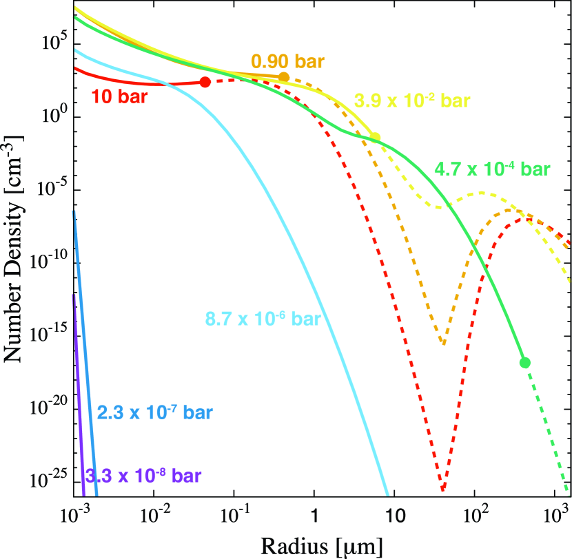
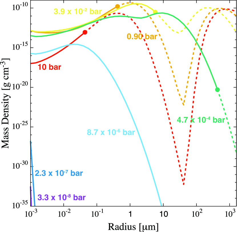
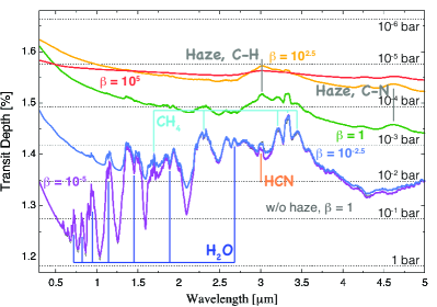
Figure 14 shows the transmission spectrum models for the atmosphere with haze for the five cases where is (red line), (yellow line), (green line, same as the green line in Fig. 9), (blue line), and (purple line). Transmission spectrum model for the atmosphere without haze in the case of (black line) is also plotted, but can be hardly seen as it overlaps with that for the atmosphere with haze for (purple line). Similarly to Fig. 9, the horizontal dotted lines represent the transit depths corresponding to the pressure levels from bar to bar for the atmosphere in the case of . From this figure, we can see that the transmission spectrum varies with the value of significantly. In the case of (red line), the overall spectrum is rather flat. This is because the floating haze particles at high altitudes ( bar) make the atmosphere so optically thick that their absorption obscures spectral absorption features due to the molecules in the lower ( bar) atmosphere. Also, it turns out that the bimodal size distribution seen in the range of bar (see Fig. 11) hardly affects the resultant transmission spectrum. In the case of (yellow line), some features of the haze can been seen, which include the spectral slope due to Rayleigh scattering in the optical and the absorption features at 3.0 and 4.6 coming from the vibrational transitions of the C-H and CN bonds, respectively. As decreases, the overall transit depth becomes lower. This is because the altitude at which the atmosphere becomes optically thick also decreases. In the case of (purple line), the spectrum is almost the same as that of the atmosphere without haze (black line). In conclusion, these results demonstrate that the difference in monomer production rate, which relates to the UV irradiation intensity from the host star, makes the diversity of transmission spectrum: completely flat spectrum, spectrum with only extinction features of hazes (i.e., spectral slope due to Rayleigh scattering and absorption features of hazes), spectrum with slope due to Rayleigh scattering and some molecular absorption features, and spectrum with only molecular absorption features.
4 Validity of characteristic size approximation in Particle Growth Calculation
When comparing theoretical transmission spectra of hazy atmospheres with high-precision observational data, the distribution of haze particles has to be determined with multiple-size growth calculations ( 2.2). To explore the possibility of reducing the computational cost and understand the effect of bimodality on transmission spectra, we examine the validity of characteristic size approximation quantitatively, applying the grain growth model of Ormel (2014). The characteristic size approximation assumes that there are particles of a single size and monomers in the atmosphere. This approximation is validated, at least, in the studies of the dynamics of dust grains in protoplanetary disks (Okuzumi et al., 2011) and proto-envelopes of gas giants (Ormel, 2014).
We assume that the haze particle size distribution at any altitude is characterized by a characteristic mass , defined as (Ormel, 2014)
| (70) |
where is the distribution function of particles of mass . The characteristic mass changes by both coagulation of haze particles and production of monomers. The latter effect decreases the value of toward the monomer mass. In this study, because focusing on the effect of size distribution, we neglect the gravitational collection and eddy diffusion, which are included in our particle growth module developed in 2.2. Thus, we assume that coagulation occurs due to the Brownian collision only. The gravitational collection is important when both small and large particles are abundant. Thus, as shown in the previous section, this has a significant influence on the vertical profile of haze particles in the case of . However, as also shown above because the altitude where gravitational collection becomes important is optically thick enough for transmitted radiation, the exclusion of gravitational collection has a little effect on resultant transmission spectra. Also, as the particle transport mechanism, we take only gravitational sedimentation into account and ignore eddy diffusion. While the eddy diffusion affects the vertical profile of haze particles in the lower atmosphere in the case of to some extent, we ignore the effect because we want to focus on the effect of size distribution. The maximum differences in transit depth between spectrum models obtained from the multiple size calculations with and without two effects (gravitational collection and eddy diffusion) in the wavelength range of 0.3-5 m are 38, 64, 43, 202, and 85ppm for , , , , and , respectively. The relatively large difference for case comes from the eddy diffusion effect.
Figure 15 shows the transmission spectrum models for the atmosphere with haze for the five cases where is (red line), (yellow line), (green line), (blue line), and (purple line). Models obtained from the multiple size calculations ( 2.2) are shown with thick lines, while those calculated with the characteristic size approximation are plotted with thin lines. The model for the haze-free atmosphere for (black line) is also plotted. Same as Fig. 9, the horizontal dotted lines represent the transit depths corresponding to the pressure levels from bar to bar for the atmosphere without haze in the case of . Again, we ignore the gravitational collection and eddy diffusion also in the multiple-size particle growth calculations to compare the results from those with the characteristic size approximation.
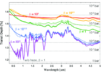
In the case of (red lines), although the size distribution is obviously bimodal in the lower atmosphere (see Figs. 12 and 13), the difference between the two spectrum models are very small. This is because haze particles are so abundant that the atmosphere is optically thick at low pressures ( bar) and therefore the difference in haze particle distribution in the lower atmosphere ( bar) hardly affects the resultant spectrum. In the case of the intermediate values of (yellow lines), (green lines), and (blue lines), the differences between the two models are relatively large, because the size multiplicity is important. In the case of (purple lines), the difference in transit depth between the two models are relatively small because of their small abundance of haze in the atmosphere.
The maximum differences in transit depth between the two models in the wavelength range of 0.3-5 m for , , , , and are 87, 205, 393, 393, and 101ppm, respectively. Precision of observed transit depths depends on properties of the planet, host star, observational instrument, and so on. If the precision of observed transit depths is larger than the difference in transit depth between the multiple-size and characteristic-size models, the characteristic size approximation is useful.
5 Summary and Conclusions
In this study, we have developed the transmission spectrum models of a close-in warm ( 500 K) exoplanet with a hazy hydrogen-dominated atmosphere by calculating directly the creation, growth, and settling of hydrocarbon haze particles to derive the distribution of haze particles. More specifically, we have done photochemical calculations to derive the vertical profiles of volume mixing ratios of the haze precursors, HCN and . Then, using the obtained vertical profiles of the precursors, we have calculated the growth and settling of haze particles in the atmosphere to derive the steady-state distribution of the size and number density of haze particles. We have also modeled transmission spectra of the atmospheres with obtained properties of hazes to explore whether the recently-observed diversity of transmission spectra can be explained by the variation in the production rate of haze monomers.
We have found that the haze particles tend to distribute in a wider region than previously assumed and consists of various sizes. We have also found that the difference in the production rate of haze monomers, which relates to the UV irradiation intensity from the host star, yields the diversity of transmission spectra observationally suggested: completely flat spectra, spectra with only extinction features of hazes (i.e., spectral slope due to Rayleigh scattering and absorption features of hazes), spectra with slope due to Rayleigh scattering and some molecular absorption features, and spectra with only molecular absorption features.
Also, by applying the grain growth model of Ormel (2014), we have examined the validity of characteristic size approximation in particle growth calculation. We have quantified the precisions of observed transit depths beyond which the characteristic approximation suffices to be used for comparison with observation.
In this paper, we have focused mainly on describing the methodology and demonstrating the sensitivity of transmission spectra to haze monomer production rate. In our forthcoming papers, we make detailed investigation of the dependence of transmission spectra on model parameters other than monomer production rate such as atmospheric metallicity, C/O ratio, eddy diffusion coefficient, atmospheric temperature profile, and monomer size. Also, we explore in detail the composition of the atmospheres of known warm exoplanets by comparing the observed spectra with our theoretical ones, taking into account other possibilities of cloud/haze constituents.
Appendix A Comparison with Tsai et al. (2017)
To verify our photochemical model presented in section 2.1, we first examine our thermochemical reaction networks. In this section, we attempt to reproduce the results of Tsai et al. (2017) for two hot Jupiters, HD 189733b and HD 209458b. They considered thermochemistry and eddy-diffusion transport, but ignored photochemistry. They then simulated the atmospheric chemistry of these two planets to compare their models with those of Moses et al. (2011).
For comparison, we adopt the same assumptions and values of input parameters that Tsai et al. (2017) adopted: The fluxes of all the species are zero both at the lower and upper boundaries. The temperature profiles are the dayside-averaged ones taken from the supplementary material of Moses et al. (2011). The value of eddy diffusion coefficient is and the solar elemental abundance ratios from Table 10 of Lodders et al. (2009). O abundance is multiplied by a factor of 0.793 to account for the effect of oxygen sequestration (see Moses et al., 2011). We prepare 90 layers with thickness of 50 km and 140 km for the simulations of HD 189733b and HD 209458b, respectively, and place the lower boundary pressure at 1000 bar. For the values of planet mass and 1000-bar radius, we use 1.15 and 1.26 for HD 189733b (Bouchy et al., 2005), and 0.685 and 1.359 for HD 209458b (Torres et al., 2008).
Figure 16 shows the calculated vertical distributions of gaseous species (solid lines) for the atmospheres of (a) HD 189733b and (b) HD 209458b, which are compared to the results of Tsai et al. (2017) (thin solid lines with crosses). HCN is not included in the model of Tsai et al. (2017), while the molecules indicated in italics are not included in our model. Vertical distributions of HCN from “no photon” models of Moses et al. (2011), in which they omit photochemistry, are also shown (thin solid lines with asterisks). We take these data by tracing their Figure 3 with the use of the software, PlotDigitizer X666http://www.surf.nuqe.nagoya-u.ac.jp/ nakahara/software/plotdigitizerx/index-e.html. We also present the thermochemical equilibrium abundances with dashed lines for reference.
In the case of (a) HD 189733b first, the mixing ratios of ours and Tsai et al. (2017) differ by a factor of 30 for , 4 for , and 2 for , because quench occurs at higher pressure in our model. Because of such difference in , our abundances of and are larger by 1-2 and 1-3 orders of magnitude, respectively. The abundances of species in thermochemical equilibrium such as , , and match theirs well. As for haze precursors, since HCN is not considered in their models, we cannot do any comparison regarding HCN. However, the “no photon” models of Moses et al. (2011) (thin solid line with asterisks), in which they omit photochemistry, yield similar abundances to ours. The abundance of differs little between Tsai et al. (2017)’s and ours. This slight difference in abundance never affects our results regarding haze distributions and transmission spectra, since the profile of the production rate of monomers is determined mainly by that of HCN abundance (see 3.1 and 3.4).
In the case of (b) HD 209458b, the abundances of the species, , , , , , , , and O, match theirs well. This is because of higher temperature of HD 209458b, for which the molecules tend to be closer to thermochemical equilibrium. As for haze precursors, we again compare the HCN abundance from our model with that from the “no photon” models of Moses et al. (2011). In our model, the abundance of HCN deviates from its thermochemical equilibrium values at higher pressure ( bar) compared to Moses et al. (2011) ( bar), and HCN results in being quenched at larger abundance in the pressure range of bar to 100 bar. If we used the result of Moses et al. (2011) as the distribution of the precursor molecules, we would assume smaller monomer production at high altitudes and larger at low altitudes. This would hamper particle growth a little and result in less flat transmission spectra. The abundance of is larger than that of Tsai et al. (2017) in the region where is not in thermochemical equilibrium (i.e., bar). However, again, this difference never affects our results regarding haze distributions and transmission spectra, because the profile of the production rate of monomers is determined mainly by that of HCN abundance.
Appendix B Comparison with Kopparapu et al. (2012)
In this section, we compare our photochemical model with the model of Kopparapu et al. (2012) for the hot Jupiter WASP-12b, in which photochemistry is considered in addition to thermochemistry and transport by eddy diffusion.
For comparison, we use the same profiles of temperature and eddy diffusion coefficient by tracing the Figure 1 of Kopparapu et al. (2012) with use of PlotDigitizer X. Following them, we neglect transport of the short-lived species and . Since the photodissociation reactions for CO, , , and are not taken into account in their model, we exclude photochemical reactions, P7, P10, P11, and P12, from our photochemical reaction list used in this section. Also, while we consider the following photochemical reaction,
which they do not consider, they consider the following photochemical reaction,
which we do not consider. The other photochemical reactions are identical to theirs. Following them, we use the G0V star spectrum from Pickles (1998) and convert it to suit for WASP-12 by using the relation between the flux at 5556 Å and the visual magnitude, , from Gray (1992). We use (Hebb et al., 2009), 427 pc as the distance to the star (Chan et al., 2011), and 0.0229 AU as the semi-major axis (Hebb et al., 2009). We take the solar elemental abundance ratios from Table 1 of Asplund et al. (2005) following them. We prepare 100 layers with thickness of 128 km placing the lower boundary pressure at 1 bar. For the values of planet mass and 1-bar radius, we use 1.41 and 1.79 , respectively (Hebb et al., 2009).
Figure 17 shows the calculated vertical distributions of gaseous species (solid lines), which are compared to the results of Kopparapu et al. (2012) (solid lines with symbols) that we also take by tracing their Figure 4 with the use of PlotDigitizer X. We also present the thermochemical equilibrium abundances with dashed lines for reference.
The abundances of the major () species agree with Kopparapu et al. (2012)’s within one order of magnitude. The abundances at the lower boundary (1 bar) are slightly different from theirs, although we have used thermochemical equilibrium values for the lower boundary condition in the same way as they did and also used the same elemental abundance ratios. The differences in abundance profile may come from those in these lower boundary values.
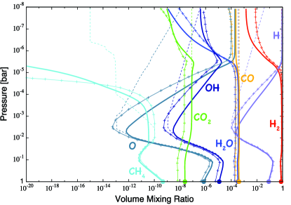
Appendix C Thermochemical Reactions
| No. | No. HuaaReaction number of Hu et al. (2012) | Reactants | Products | Rate Coefficients bbUnit of for 2-body reactions and for 3-body reactions | Ref. | Temp.ccUnit of | |
|---|---|---|---|---|---|---|---|
| R1 | R1 | NIST | 1000-4000 | ||||
| R2 | R2 | NIST | 5000-8000 | ||||
| R3 | R3 | NIST | 1520-2540 | ||||
| R4 | R5 | NIST | 2000-5000 | ||||
| R5 | R6 | NIST | 15-295 | ||||
| R6 | R14 | NIST | 300-2500 | ||||
| R7 | R17 | NIST | 294 | ||||
| R8 | R31 | NIST | 298 | ||||
| R9 | R34 | NIST | 300-2500 | ||||
| R10 | R40 | NIST | 298-3000 | ||||
| R11 | R42 | NIST | 1100-2700 | ||||
| R12 | R43 | NIST | 1100-2700 | ||||
| R13 | R48 | NIST | 296-707 | ||||
| R14 | R49 | NIST | 300-2500 | ||||
| R15 | R50 | NIST | 300-2500 | ||||
| R16 | R57 | NIST | 300-2500 | ||||
| R17 | R69 | NIST | 300-2500 | ||||
| R18 | R71 | NIST | 300-2500 | ||||
| R19 | R91 | NIST | 300-2500 | ||||
| R20 | R96 | NIST | 300-2500 | ||||
| R21 | R99 | NIST | 290-1500 | ||||
| R22 | R101 | NIST | 294 | ||||
| R23 | R108 | NIST | 300-2500 | ||||
| R24 | R113 | NIST | 300-2500 | ||||
| R25 | R116 | NIST | 500-2500 | ||||
| R26 | R120 | NIST | 300-2500 | ||||
| R27 | R122 | NIST | 1500-1900 | ||||
| R28 | R127 | NIST | 300-2500 | ||||
| R29 | R128 | NIST | 300-2500 | ||||
| R30 | R129 | NIST | 300-2500 | ||||
| R31 | R145 | NIST | 300-2000 | ||||
| R32 | R146 | NIST | 300-3000 | ||||
| R33 | R149 | NIST | 300-2500 | ||||
| R34 | R152 | NIST | 300-2500 | ||||
| R35 | R153 | NIST | 300-2500 | ||||
| R36 | R157 | NIST | 300-2500 | ||||
| R37 | R158 | NIST | 1370-1840 | ||||
| R38 | R159 | NIST | 300-2500 | ||||
| R39 | R162 | NIST | 300-2500 | ||||
| R40 | R165 | NIST | 300-2500 | ||||
| R41 | R166 | NIST | 300-2500 | ||||
| R42 | R184 | NIST | 1500-2500 | ||||
| R43 | R185 | NIST | 1100-1800 | ||||
| R44 | R186 | NIST | 490-1780 | ||||
| R45 | R191 | NIST | 800-3500 | ||||
| R46 | R193 | NIST | 1520-2540 | ||||
| R47 | R194 | NIST | 2580-4650 | ||||
| R48 | R195 | NIST | 200-2000 | ||||
| R49 | R202 | NIST | 327-397 | ||||
| R50 | R203 | NIST | 300-2500 | ||||
| R51 | R204 | NIST | 300-2500 | ||||
| R52 | R207 | NIST | 300-2500 | ||||
| R53 | R211 | NIST | 833-1432 | ||||
| R54 | R212 | NIST | 400-2200 | ||||
| R55 | R214 | NIST | 1000-4000 | ||||
| R56 | R215 | NIST | 300-2000 | ||||
| R57 | R218 | NIST | 298-669 | ||||
| R58 | R219 | NIST | 500-2500 | ||||
| R59 | R276 | NIST | 298 | ||||
| R60 | R280 | NIST | 990-1010 | ||||
| R61 | R281 | NIST | 216-584 | ||||
| R62 | R282 | NIST | 200-423 | ||||
| R63 | R284 | NIST | 300-2500 | ||||
| R64 | R287 | NIST | 800-3000 | ||||
| R65 | R289 | NIST | 300-2500 | ||||
| R66 | R290 | NIST | 1000-4000 | ||||
| R67 | R300 | NIST | 1300-1700 | ||||
| R68 | R305 | NIST | 250-3000 | ||||
| R69 | R309 | NIST | 298-3000 | ||||
| R70 | R310 | NIST | 1000-4000 | ||||
| R71 | R311 | NIST | 340-510 | ||||
| R72 | R316 | NIST | 300-2000 | ||||
| R73 | R317 | NIST | 300-2000 | ||||
| R74 | R319 | NIST | 300-3000 | ||||
| R75 | R323 | NIST | 298-3000 | ||||
| R76 | R326 | NIST | 250-3000 | ||||
| R77 | R327 | NIST | 300-1300 | ||||
| R78 | R328 | NIST | 350-600 | ||||
| R79 | R329 | NIST | 300-700 | ||||
| R80 | R388 | NIST | 8000 | ||||
| R81 | R389 | NIST | 300-2500 | ||||
| R82 | R391 | NIST | 300-2500 | ||||
| R83 | R407 | NIST | 10-6000 | ||||
| R84 | R408 | NIST | 300-2000 | ||||
| R85 | R409 | NIST | 300-2500 | ||||
| R86 | R410 | NIST | 1200-1800 | ||||
| R87 | R411 | NIST | 300-2500 | ||||
| R88 | R412 | NIST | 300-2500 | ||||
| R89 | R414 | NIST | 300-2500 | ||||
| R90 | R416 | NIST | 290-900 | ||||
| R91 | R420 | NIST | 298 | ||||
| R92 | R423 | NIST | 420-1520 | ||||
| R93 | R424 | NIST | 300-1000 | ||||
| R94 | R426 | NIST | 300-2500 | ||||
| R95 | R427 | NIST | 300-2500 | ||||
| R96 | R430 | NIST | 500-2500 | ||||
| R97 | R433 | NIST | 300-2500 | ||||
| R98 | R436 | JPL | 470-900 | ||||
| R99 | R445 | JPL | 200-300 | ||||
| R100 | R449 | JPL | 200-300 | ||||
| R101 | R450 | JPL | 200-300 | ||||
| R102 | R453 | NIST | 300 | ||||
| R103 | R454 | JPL | 200-300 | ||||
| R104 | R455 | JPL | 200-300 | ||||
| R105 | R456 | JPL | 200-300 | ||||
| R106 | R458 | JPL | 200-300 | ||||
| R107 | R461 | JPL | 200-300 | ||||
| R108 | R464 | JPL | 200-300 | ||||
| R109 | R476 | NIST | 2200 | ||||
| R110 | R477 | NIST | 300-2500 | ||||
| R111 | R478 | NIST | 300-2500 | ||||
| R112 | R480 | NIST | 300-2500 | ||||
| R113 | R482 | NIST | 500-2500 | ||||
| R114 | R495 | NIST | 300-3000 | ||||
| R115 | R496 | NIST | 300-1000 | ||||
| R116 | R501 | JPL | 200-300 | ||||
| R117 | R502 | JPL | 200-300 | ||||
| R118 | R504 | NIST | 300-2500 | ||||
| R119 | R507 | NIST | 500-2500 | ||||
| R120 | R511 | NIST | 300-2000 | ||||
| R121 | R512 | JPL | 200-300 | ||||
| R122 | R515 | NIST | 500-2500 | ||||
| R123 | R516 | NIST | 298-2840 | ||||
| R124 | R523 | JPL | 200-300 | ||||
| R125 | R526 | JPL | 200-300 | ||||
| R126 | R596 | YD99ddYung & Demore (1999) | |||||
| R127 | R597 | YD99ddYung & Demore (1999) | |||||
| R128 | R598 | YD99ddYung & Demore (1999) | |||||
| R129 | R599 | YD99ddYung & Demore (1999) | |||||
| R130 | R608 | YD99ddYung & Demore (1999) | |||||
| R131 | R644 | NIST | 250-3000 | ||||
| R132 | M1 | NIST | 5000-6000 | ||||
| R133 | M2 | NIST | 300 | ||||
| R134 | M11 | NIST | 500-2500 | ||||
| R135 | M12 | NIST | 300-2500 | ||||
| R136 | M13 | NIST | 300-2500 | ||||
| R137 | M14 | NIST | 298 | ||||
| R138 | M16 | NIST | 300-2500 | ||||
| R139 | M18 | NIST | 300-3000 | ||||
| R140 | M22 | NIST | 298 | ||||
| R141 | M23 | NIST | 298 | ||||
| R142 | M24 | NIST | 298 | ||||
| R143 | M25 | JPL | 90-6400 | ||||
| R144 | M30 | NIST | 8000 | ||||
| R145 | M31 | NIST | 300-2500 | ||||
| R146 | M34 | NIST | 200-4000 | ||||
| R147 | M55 | YD99ddYung & Demore (1999) | |||||
| R148 | M56 | NIST | 300-1000 | ||||
| R149 | M72 | eeRate coefficient : | YD99ddYung & Demore (1999) | ||||
| R150 | T19 | NIST | 1400-2500 | ||||
| R151 | T20 | NIST | 1000-2000 | ||||
| R152 | T22 | NIST | 1000-3000 | ||||
| R153 | T46 | NIST | 298-1229 | ||||
| R154 | T57 | NIST | 1800-5000 |
Note. — Thermochemical Reactions used in our photochemical model. refers to the number density of background atmosphere (unit of ). We assume equals to the total number density.
Appendix D Photochemical Reactions
| No. | No. HuaaReaction number of Hu et al. (2012) | Reactants | Products | Quantum Yields | |
|---|---|---|---|---|---|
| P1 | 1 | nm: 0.5 | |||
| nm nm: 0 | |||||
| nm: 1.0 | |||||
| P2 | 2 | nm: 0.5 | |||
| nm nm: 1.0 | |||||
| nm: 0 | |||||
| P3 | 6 | ||||
| P4 | 32 | 0.41 (Smith & Raulin, 1999) | |||
| P5 | 33 | 0.53 (Smith & Raulin, 1999) | |||
| P6 | 34 | 0.06 (Smith & Raulin, 1999) | |||
| P7 | 35 | nm: 1.0 | |||
| nm: 0 | |||||
| P8 | 36 | nm: 0 | |||
| nm nm: 1.0 | |||||
| nm: 0 | |||||
| P9 | 37 | nm: 1.0 | |||
| nm: 0 | |||||
| P10 | 38 | nm: 0.1 (Mentall & Gentieu, 1970) | |||
| nm nm: 1.0 | |||||
| nm: 0 | |||||
| P11 | 39 | 1.0 | |||
| P12 | 40 | 1.0 | |||
| P13 | 41 | 1.0 | |||
| P14 | 42 | nm: 0.3 (Lilly et al., 1973) | |||
| nm nm: Linear interpolation | |||||
| nm: 1.0 | |||||
| P15 | 43 | nm: 0.7 | |||
| nm nm: Linear interpolation | |||||
| nm: 1.0 | |||||
| P16 | 55 | nm: 1.0 (Läuter et al., 2002) | |||
| nm: 0 |
Note. — Photochemical Reactions used in our photochemical model and values of quantum yields.
Appendix E UV Cross Sections
| Species | Wavelength | Cross Sections | TaaTemperature dependence: Y and N indicate whether temperature dependence is taken into account or not. |
|---|---|---|---|
| nm nm | Brion et al. (1979) | N | |
| nm nm | Ogawa & Ogawa (1975) | N | |
| nm nm | Yoshino et al. (2005) | N | |
| nm nm | Kockarts (1976) | N | |
| nm nm | Sander et al. (2011) | N | |
| nm nm | Chan et al. (1993b) | N | |
| nm nm | Sander et al. (2011) | N | |
| nm nm | Extrapolation | ||
| nm nm | Kameta et al. (2002) | N | |
| nm nm | Chen & Wu (2004) | N | |
| nm nm | Lee et al. (2001) | N | |
| nm nm | Chan et al. (1993a) | N | |
| nm nm | Huestis & Berkowitz (2010) | N | |
| nm nm | Ityaksov et al. (2008) | N | |
| nm nm | Lee et al. (1976) | N | |
| nm nm | Cook & Metzger (1964) | N | |
| nm nm | Backx et al. (1976) | N | |
| nm nm | Chan et al. (1993c) | N | |
| nm nm | Burton et al. (1992) | N | |
| nm nm | Nee et al. (1985) | N | |
| nm nm | Cheng et al. (2002) | N | |
| nm nm | Macpherson & Simons (1978) | N | |
| nm nm | Samson et al. (1987) | N | |
| nm nm | Wu et al. (2007) | N | |
| nm nm | Cheng et al. (2006) | N | |
| nm nm | Cooper et al. (1995) | N | |
| nm nm | Smith et al. (1991) | Y | |
| nm nm | Bénilan et al. (2000) | Y |
References
- Allen et al. (1981) Allen, M., Yung, Y. L., & Waters, J. W. 1981, J. Geophys. Res., 86, 3617
- Anglada-Escudé et al. (2013) Anglada-Escudé, G., Rojas-Ayala, B., Boss, A. P., Weinberger, A. J., & Lloyd, J. P. 2013, A&A, 551, A48
- Armitage (2010) Armitage, P. J. . 2010, Astrophysics of Planet Formation (New York: Cambridge University Press)
- Asplund et al. (2005) Asplund, M., Grevesse, N., & Sauval, A. J. 2005, in Astronomical Society of the Pacific Conference Series, Vol. 336, Cosmic Abundances as Records of Stellar Evolution and Nucleosynthesis, ed. T. G. Barnes, III & F. N. Bash, 25
- Awiphan et al. (2016) Awiphan, S., Kerins, E., Pichadee, S., et al. 2016, MNRAS, 463, 2574
- Backx et al. (1976) Backx, C., Wight, G. R., & Van der Wiel, M. J. 1976, Journal of Physics B Atomic Molecular Physics, 9, 315
- Bénilan et al. (2000) Bénilan, Y., Smith, N., Jolly, A., & Raulin, F. 2000, Planet. Space Sci., 48, 463
- Biddle et al. (2014) Biddle, L. I., Pearson, K. A., Crossfield, I. J. M., et al. 2014, MNRAS, 443, 1810
- Bohren & Huffman (2004) Bohren, C. F., & Huffman, D. R. 2004, Absorption and Scattering of Light by Small Particles (Weinheim: Wiley-VCH)
- Bouchy et al. (2005) Bouchy, F., Udry, S., Mayor, M., et al. 2005, A&A, 444, L15
- Brion et al. (1979) Brion, C., Tan, K., van der Wiel, M., & van der Leeuw, P. 1979, Journal of Electron Spectroscopy and Related Phenomena, 17, 101
- Brown (2001) Brown, T. M. 2001, ApJ, 553, 1006
- Burton et al. (1992) Burton, G. R., Chan, W. F., Cooper, G., & Biron, C. E. 1992, Chemical Physics, 167, 349
- Cantrell et al. (2013) Cantrell, J. R., Henry, T. J., & White, R. J. 2013, AJ, 146, 99
- Chan et al. (2011) Chan, T., Ingemyr, M., Winn, J. N., et al. 2011, AJ, 141, 179
- Chan et al. (1993a) Chan, W. F., Cooper, G., & Brion, C. E. 1993a, Chemical Physics, 170, 123
- Chan et al. (1993b) —. 1993b, Chemical Physics, 178, 387
- Chan et al. (1993c) Chan, W. F., Cooper, G., Sodhi, R. N. S., & Brion, C. E. 1993c, Chemical Physics, 170, 81
- Charbonneau et al. (2009) Charbonneau, D., Berta, Z. K., Irwin, J., et al. 2009, Nature, 462, 891
- Chen & Wu (2004) Chen, F. Z., & Wu, C. Y. R. 2004, J. Quant. Spec. Radiat. Transf., 85, 195
- Cheng et al. (2002) Cheng, B.-M., Bahou, M., Lee, Y.-P., & Lee, L. C. 2002, Journal of Geophysical Research (Space Physics), 107, 1161
- Cheng et al. (2006) Cheng, B.-M., Lu, H.-C., Chen, H.-K., et al. 2006, ApJ, 647, 1535
- Cook & Metzger (1964) Cook, G. R., & Metzger, P. H. 1964, Journal of the Optical Society of America (1917-1983), 54, 968
- Cooper et al. (1995) Cooper, G., Olney, T. N., & Brion, C. E. 1995, Chemical Physics, 194, 175
- Crossfield et al. (2013) Crossfield, I. J. M., Barman, T., Hansen, B. M. S., & Howard, A. W. 2013, A&A, 559, A33
- Davies (1945) Davies, C. N. 1945, Proceedings of the Physical Society, 57, 259
- de Mooij et al. (2012) de Mooij, E. J. W., Brogi, M., de Kok, R. J., et al. 2012, A&A, 538, A46
- Dragomir et al. (2015) Dragomir, D., Benneke, B., Pearson, K. A., et al. 2015, ApJ, 814, 102
- Ehrenreich et al. (2014) Ehrenreich, D., Bonfils, X., Lovis, C., et al. 2014, A&A, 570, A89
- Fischer et al. (2003) Fischer, J., Gamache, R. R., Goldman, A., Rothman, L. S., & Perrin, A. 2003, J. Quant. Spec. Radiat. Transf., 82, 401
- Fortney et al. (2007) Fortney, J. J., Marley, M. S., & Barnes, J. W. 2007, ApJ, 659, 1661
- France et al. (2016) France, K., Parke Loyd, R. O., Youngblood, A., et al. 2016, ApJ, 820, 89
- Fukui et al. (2013) Fukui, A., Narita, N., Kurosaki, K., et al. 2013, ApJ, 770, 95
- Fukui et al. (2014) Fukui, A., Kawashima, Y., Ikoma, M., et al. 2014, ApJ, 790, 108
- Fukui et al. (2016) Fukui, A., Narita, N., Kawashima, Y., et al. 2016, ApJ, 819, 27
- Grassi et al. (2014) Grassi, T., Bovino, S., Schleicher, D. R. G., et al. 2014, MNRAS, 439, 2386
- Gray (1992) Gray, D. F. 1992, The observation and analysis of stellar photospheres.
- Guillot (2010) Guillot, T. 2010, A&A, 520, A27
- Haynes (2012) Haynes, W. M. 2012, CRC HANDBOOK OF CHEMISTRY and PHYSICS, 92nd edn. (CRC Press)
- Hebb et al. (2009) Hebb, L., Collier-Cameron, A., Loeillet, B., et al. 2009, ApJ, 693, 1920
- Helling & Woitke (2006) Helling, C., & Woitke, P. 2006, A&A, 455, 325
- Heng (2016) Heng, K. 2016, ApJ, 826, L16
- Heng & Kitzmann (2017) Heng, K., & Kitzmann, D. 2017, MNRAS, 470, 2972
- Hindmarsh (1982) Hindmarsh, A. C. 1982, IMACS Trans. Sci. Comput., 1, 55
- Howe & Burrows (2012) Howe, A. R., & Burrows, A. S. 2012, ApJ, 756, 176
- Hu et al. (2012) Hu, R., Seager, S., & Bains, W. 2012, ApJ, 761, 166
- Huestis & Berkowitz (2010) Huestis, D. L., & Berkowitz, J. 2010, in Bulletin of the American Astronomical Society, Vol. 42, AAS/Division for Planetary Sciences Meeting Abstracts #42, 972
- Husser et al. (2013) Husser, T.-O., Wende-von Berg, S., Dreizler, S., et al. 2013, A&A, 553, A6
- Ityaksov et al. (2008) Ityaksov, D., Linnartz, H., & Ubachs, W. 2008, Chemical Physics Letters, 462, 31
- Jacobson (2005) Jacobson, M. Z. M. Z. 2005, Fundamentals of atmospheric modeling / Mark Z. Jacobson, 2nd edn., Vol. : pbk; : hard (New York: Cambridge University Press), xiv, 813 p.
- Kameta et al. (2002) Kameta, K., Kouchi, N., Ukai, M., & Hatano, Y. 2002, Journal of Electron Spectroscopy and Related Phenomena, 123, 225 , determination of cross-sections and momentum profiles of atoms, molecules and condensed matter
- Khare et al. (1984) Khare, B. N., Sagan, C., Arakawa, E. T., et al. 1984, Icarus, 60, 127
- Knutson et al. (2014) Knutson, H. A., Benneke, B., Deming, D., & Homeier, D. 2014, Nature, 505, 66
- Kockarts (1976) Kockarts, G. 1976, Planet. Space Sci., 24, 589
- Kopparapu et al. (2012) Kopparapu, R. k., Kasting, J. F., & Zahnle, K. J. 2012, ApJ, 745, 77
- Kreidberg et al. (2014) Kreidberg, L., Bean, J. L., Désert, J.-M., et al. 2014, Nature, 505, 69
- Kuntz (1997) Kuntz, M. 1997, J. Quant. Spec. Radiat. Transf., 57, 819
- Lanotte et al. (2014) Lanotte, A. A., Gillon, M., Demory, B.-O., et al. 2014, A&A, 572, A73
- Läuter et al. (2002) Läuter, A., Lee, K. S., Jung, K. H., et al. 2002, Chemical Physics Letters, 358, 314
- Lavvas et al. (2010) Lavvas, P., Yelle, R. V., & Griffith, C. A. 2010, Icarus, 210, 832
- Lecavelier Des Etangs et al. (2008) Lecavelier Des Etangs, A., Pont, F., Vidal-Madjar, A., & Sing, D. 2008, A&A, 481, L83
- Lee et al. (2001) Lee, A. Y. T., Yung, Y. L., Cheng, B.-M., et al. 2001, ApJ, 551, L93
- Lee et al. (1976) Lee, L. C., Carlson, R. W., & Judge, D. L. 1976, J. Quant. Spec. Radiat. Transf., 16, 873
- Lilly et al. (1973) Lilly, R., Rebbert, R., & Ausloos, P. 1973, Journal of Photochemistry, 2, 49
- Line et al. (2011) Line, M. R., Vasisht, G., Chen, P., Angerhausen, D., & Yung, Y. L. 2011, ApJ, 738, 32
- Linsky et al. (2014) Linsky, J. L., Fontenla, J., & France, K. 2014, ApJ, 780, 61
- Liou (2002) Liou, K. N. 2002, An Introduction to Atmospheric Radiation, 2nd edn. (Amsterdam: Academic Press)
- Lodders (2003) Lodders, K. 2003, ApJ, 591, 1220
- Lodders et al. (2009) Lodders, K., Palme, H., & Gail, H.-P. 2009, Landolt Börnstein, arXiv:0901.1149
- Loyd et al. (2016) Loyd, R. O. P., France, K., Youngblood, A., et al. 2016, ApJ, 824, 102
- Macpherson & Simons (1978) Macpherson, M. T., & Simons, J. P. 1978, J. Chem. Soc., Faraday Trans. 2, 74, 1965
- McKay et al. (2001) McKay, C. P., Coustenis, A., Samuelson, R. E., et al. 2001, Planet. Space Sci., 49, 79
- Mentall & Gentieu (1970) Mentall, J. E., & Gentieu, E. P. 1970, J. Chem. Phys., 52, 5641
- Mie (1908) Mie, G. 1908, Annalen der Physik, 330, 377
- Miguel & Kaltenegger (2014) Miguel, Y., & Kaltenegger, L. 2014, ApJ, 780, 166
- Miller-Ricci & Fortney (2010) Miller-Ricci, E., & Fortney, J. J. 2010, ApJ, 716, L74
- Miller-Ricci Kempton et al. (2012) Miller-Ricci Kempton, E., Zahnle, K., & Fortney, J. J. 2012, ApJ, 745, 3
- Morley et al. (2013) Morley, C. V., Fortney, J. J., Kempton, E. M.-R., et al. 2013, ApJ, 775, 33
- Moses et al. (2011) Moses, J. I., Visscher, C., Fortney, J. J., et al. 2011, ApJ, 737, 15
- Moses et al. (2013) Moses, J. I., Line, M. R., Visscher, C., et al. 2013, ApJ, 777, 34
- Narita et al. (2013) Narita, N., Fukui, A., Ikoma, M., et al. 2013, ApJ, 773, 144
- Nascimbeni et al. (2013) Nascimbeni, V., Piotto, G., Pagano, I., et al. 2013, A&A, 559, A32
- Nascimbeni et al. (2015) Nascimbeni, V., Mallonn, M., Scandariato, G., et al. 2015, A&A, 579, A113
- Nee et al. (1985) Nee, J. B., Suto, M., & Lee, L. C. 1985, Chemical Physics, 98, 147
- Ogawa & Ogawa (1975) Ogawa, S., & Ogawa, M. 1975, Canadian Journal of Physics, 53, 1845
- Okuzumi et al. (2011) Okuzumi, S., Tanaka, H., Takeuchi, T., & Sakagami, M.-a. 2011, ApJ, 731, 95
- Ormel (2014) Ormel, C. W. 2014, ApJ, 789, L18
- Petty (2006) Petty, G. W. 2006, A First Course in Atmospheric Radiation, 2nd edn. (Madison, Wis.: Sundog Pub.)
- Pickles (1998) Pickles, A. J. 1998, PASP, 110, 863
- Rothman et al. (1998) Rothman, L. S., Rinsland, C. P., Goldman, A., et al. 1998, J. Quant. Spec. Radiat. Transf., 60, 665
- Rothman et al. (2013) Rothman, L. S., Gordon, I. E., Babikov, Y., et al. 2013, J. Quant. Spec. Radiat. Transf., 130, 4
- Ruyten (2004) Ruyten, W. 2004, J. Quant. Spec. Radiat. Transf., 86, 231
- Samson et al. (1987) Samson, J. A. R., Haddad, G. N., & Kilcoyne, L. D. 1987, J. Chem. Phys., 87, 6416
- Sander et al. (2011) Sander, S. P., Friedl, R. R., Abbatt, J. P. D., et al. 2011, Chemical Kinetics and Photochemical Data for Use in Atmospheric Studies Evaluation Number 17 (JPL Publication)
- Seager & Deming (2010) Seager, S., & Deming, D. 2010, ARA&A, 48, 631
- Sharp & Burrows (2007) Sharp, C. M., & Burrows, A. 2007, ApJS, 168, 140
- Sing et al. (2015) Sing, D. K., Wakeford, H. R., Showman, A. P., et al. 2015, MNRAS, 446, 2428
- Sing et al. (2016) Sing, D. K., Fortney, J. J., Nikolov, N., et al. 2016, Nature, 529, 59
- Smith & Raulin (1999) Smith, N. S., & Raulin, F. 1999, J. Geophys. Res., 104, 1873
- Smith et al. (1991) Smith, P. L., Yoshino, K., Parkinson, W. H., Ito, K., & Stark, G. 1991, J. Geophys. Res., 96, 17
- Smith et al. (2001) Smith, R. K., Brickhouse, N. S., Liedahl, D. A., & Raymond, J. C. 2001, ApJ, 556, L91
- Smith & Missen (1982) Smith, W. R., & Missen, R. W. 1982, Chemical Reaction Equilibrium Analysis: Theory and Algorithms (New York: A Wiley-Interscience Publication)
- Stevenson (2016) Stevenson, K. B. 2016, ApJ, 817, L16
- Tomasko et al. (2009) Tomasko, M. G., Doose, L. R., Dafoe, L. E., & See, C. 2009, Icarus, 204, 271
- Toon et al. (1992) Toon, O. B., McKay, C. P., Griffith, C. A., & Turco, R. P. 1992, Icarus, 95, 24
- Toon et al. (1980) Toon, O. B., Turco, R. P., & Pollack, J. B. 1980, Icarus, 43, 260
- Torres et al. (2008) Torres, G., Winn, J. N., & Holman, M. J. 2008, ApJ, 677, 1324
- Trainer et al. (2006) Trainer, M. G., Pavlov, A. A., Dewitt, H. L., et al. 2006, Proceedings of the National Academy of Science, 103, 18035
- Tsai et al. (2017) Tsai, S.-M., Lyons, J. R., Grosheintz, L., et al. 2017, ApJS, 228, 20
- Venot et al. (2014) Venot, O., Agúndez, M., Selsis, F., Tessenyi, M., & Iro, N. 2014, A&A, 562, A51
- Venot et al. (2015) Venot, O., Hébrard, E., Agúndez, M., Decin, L., & Bounaceur, R. 2015, A&A, 577, A33
- Venot et al. (2012) Venot, O., Hébrard, E., Agúndez, M., et al. 2012, A&A, 546, A43
- Visscher & Moses (2011) Visscher, C., & Moses, J. I. 2011, ApJ, 738, 72
- Woitke & Helling (2003) Woitke, P., & Helling, C. 2003, A&A, 399, 297
- Woitke & Helling (2004) —. 2004, A&A, 414, 335
- Wu et al. (2007) Wu, Y.-J., Lu, H.-C., Chen, H.-K., et al. 2007, J. Chem. Phys., 127, 154311
- Yoshino et al. (2005) Yoshino, K., Parkinson, W. H., Ito, K., & Matsui, T. 2005, Journal of Molecular Spectroscopy, 229, 238
- Youngblood et al. (2016) Youngblood, A., France, K., Parke Loyd, R. O., et al. 2016, ApJ, 824, 101
- Yung et al. (1984) Yung, Y. L., Allen, M., & Pinto, J. P. 1984, ApJS, 55, 465
- Yung & Demore (1999) Yung, Y. L., & Demore, W. B., eds. 1999, Photochemistry of planetary atmospheres
- Zahnle et al. (2016) Zahnle, K., Marley, M. S., Morley, C. V., & Moses, J. I. 2016, ApJ, 824, 137
- Zahnle & Marley (2014) Zahnle, K. J., & Marley, M. S. 2014, ApJ, 797, 41