Identifying the subtle signatures of feedback from distant AGN using ALMA observations and the EAGLE hydrodynamical simulations

Abstract

We present sensitive 870 $\mu$m continuum measurements from our ALMA programmes of 114 X-ray selected AGN in the CDF-S and COSMOS fields. We use these observations in combination with data from Spitzer and Herschel to construct a sample of 86 X-ray selected AGN, 63 with ALMA constraints at $z=1.5-3.2$ with stellar mass $>2\times 10^{10}$ $M_{\odot}$. We constructed broad-band spectral energy distributions in the infrared band (8 – 1000 $\mu$m) and constrain star-formation rates (SFRs) uncontaminated by the AGN. Using a hierarchical Bayesian method that takes into account the information from upper limits, we fit SFR and specific SFR (sSFR) distributions. We explore these distributions as a function of both X-ray luminosity and stellar mass. We compare our measurements to two versions of the EAGLE hydrodynamical simulations: the reference model with AGN feedback and the model without AGN. We find good agreement between the observations and that predicted by the EAGLE reference model for the modes and widths of the sSFR distributions as a function of both X-ray luminosity and stellar mass; however, we found that the EAGLE model without AGN feedback predicts a significantly narrower width when compared to the data. Overall, from the combination of the observations with the model predictions, we conclude that (1) even with AGN feedback, we expect no strong relationship between the sSFR distribution parameters and instantaneous AGN luminosity and (2) a signature of AGN feedback is a broad distribution of sSFRs for all galaxies (not just those hosting an AGN) with stellar masses above $\approx 10^{10}$M_⊙.

1 Introduction

The most successful models of galaxy formation require AGN activity (via “AGN feedback”) to explain many of the puzzling properties of local massive galaxies and the intergalactic medium (IGM); e.g. the colour bi-modality of local galaxies, the steep luminosity functions, the black hole–spheroid relationships and the metal enrichment of the intergalactic medium (see Alexander & Hickox, 2012; Fabian, 2012; Harrison, 2017, for reviews). The key attribute of the AGN in these models is the injection of significant energy into the interstellar medium (ISM), which inhibits or suppresses star formation by either heating the ISM or ejecting the gas out of the host galaxy through outflows (Sturm et al., 2011; Fabian, 2012; Cicone et al., 2014). In recent years it has been shown that low-redshift ($z<1$), low-accretion rate AGN are responsible for regulating the inflow of cool gas in massive galaxy clusters through heating (see McNamara & Nulsen, 2012, for review). However, despite spectroscopic observations that have shown that energetic outflows are a common property of luminous AGN (e.g. Veilleux et al., 2005; Ganguly & Brotherton, 2008; Mullaney et al., 2013; Cicone et al., 2014; Harrison et al., 2014; Balmaverde & Capetti, 2015; Harrison et al., 2016; Leung et al., 2017), we lack direct observational support that they dramatically impact on star formation in the distant Universe ($z>$ 1.5), which is a fundamental requirement for the majority of galaxy formation models (e.g. Springel et al., 2005; Vogelsberger et al., 2014; Schaye et al., 2015).

With high sensitivity at infrared (IR) wavelengths, Herschel has provided new insight into the star forming properties of distant AGN ($z>1$). The broadly accepted view is that the mean star-formation rates (SFRs) and specific SFRs (sSFRs; i.e., SFR/stellar mass) of moderate-luminosity AGN ($L_{\rm X}\approx 10^{43}$–$10^{44}$ erg s^-1) are consistent with those of the coeval star-forming galaxy population (e.g. also Lutz et al., 2010; Shao et al., 2010; Harrison et al., 2012; Mullaney et al., 2012; Santini et al., 2012; Rosario et al., 2013; Azadi et al., 2015; Stanley et al., 2015; Cowley et al., 2016). The definition of the star-forming galaxy population in this context is that of the “main sequence”; i.e., the redshift and stellar-mass dependent evolution of sSFRs of star-forming galaxies (e.g., Noeske et al., 2007; Elbaz et al., 2011; Speagle et al., 2014; Whitaker et al., 2014; Schreiber et al., 2015). To first order these results suggest a connection between AGN activity and star formation without providing clear evidence that moderate-luminosity AGN impact on star formation. By contrast, mixed results we presented for luminous AGN ($L_{\rm X}>10^{44}$ erg s^-1), with different studies arguing that AGN either suppress, enhance, or have no influence on star formation when compared to moderate-luminosity AGN (e.g. Harrison et al., 2012; Page et al., 2012; Rosario et al., 2012; Rovilos et al., 2012; Azadi et al., 2015; Stanley et al., 2015).

The majority of the current Herschel studies suffer from at least one of the following limitations, which hinder significant further progress: 1) SFRs are often calculated from single-band photometry, which doesn’t account for the factor $\approx$ 2–3 difference in the derived SFR between star forming galaxy templates (depending on wavelength; see Stanley, 2016), 2) a modest fraction of X-ray AGN are detected by Herschel (often $<10$% for X-ray AGN at $z>1.5$), which drives the majority of studies to explore the stacked average SFR rate, which can be strongly effected by bright outliers (e.g., see Mullaney et al. 2015 for solutions to this problem), 3) the contribution to the IR emission from the AGN is often not directly constrained which can be significant even for moderate-luminosity AGN (e.g. Mullaney et al., 2011; Del Moro et al., 2013), and 4) upper limits on SFRs are often ignored, which will bias reported SFRs towards high values, potentially missing key signatures of suppressed star formation. Furthermore, since mass accretion onto black holes is a stochastic process with a timescale shorter than that of star formation (e.g. Hickox et al., 2014; King & Nixon, 2015; Schawinski et al., 2015; McAlpine et al., 2017), we must be cautious about what can inferred from AGN feedback using the observed relationships between SFRs and AGN luminosities (see Harrison, 2017). To more completely constrain the impact that AGN have on star formation we need to measure (s)SFR distributions as a function of key properties (e.g., X-ray luminosity, stellar mass), which will provide more stringent tests of the current models of galaxy formation and evolution (e.g. Vogelsberger et al., 2014; Schaye et al., 2015; Lacey et al., 2016).

As described above, previous studies exploring the topic of star formation in AGN typically used linear means to estimate the SFR and sSFR of the AGN population; a single parameter description of the population. However, by using ALMA data, to go deeper than is possible with Herschel data alone, we already have shown in our pilot study (Mullaney et al., 2015) that the linear mean is consistently higher than the mode (the most common value). A linear mean of two samples can be consistent, while their distributions can be inconsistent. In that study we showed that X-ray AGN have consistent mean sSFRs but in-consistent distributions compared to main sequence galaxies. Therefore in order to adequately describe the unique star-forming properties of a population, we must constrain the parameters (the mode and the width) of the distributions of SFR or sSFR. These values are much more powerful, than a simple linear mean, to compare between different samples and to rigorously test model predictions, see §4.2.

The aim of this paper is to use sensitive ALMA observations of X-ray AGN at $z>1.5$, in conjunction with Spitzer–Herschel photometry, to address the challenges outlined above and answer the question: what impact do luminous AGN have on star formation? The significantly improved sensitivity and spatial resolution that ALMA provides over Herschel allows for the detection of star forming emission from galaxies at $z>1.5$ up to an order of magnitude below the equivalent sensitivity of Herschel (see Mullaney et al. 2015; Stanley et al, submitted). In this paper we expand on the Mullaney et al. (2015) study with additional ALMA observations of X-ray AGN to increase the overall source statistics, particularly at the high luminosity end (i.e., $L_{\rm X}>10^{44}$ erg s^-1). We also make a quantitative comparison of our results to those from a leading set of hydrodynamical cosmological simulations (EAGLE; Evolution and Assembly of GaLaxies and their Environments; Schaye et al., 2015).

In §2 we describe the data and the basic analyses used in our study, in §3 we present our main results, including a comparison to EAGLE, in §4 we discuss our results within the broader context of the impact of AGN on the star forming properties of galaxies, and in §5 we draw our conclusions. We also provide in the appendix the ALMA $870\mu$m photometry for all of the 114 X-ray sources that were either targetted in our ALMA programmes or serendipitously lay within the ALMA field of view. In all of our analyses we adopt the cosmological parameters of $\rm H_{0}=71\ km\,s^{-1}$, $\rm\Omega_{M}=0.27$, $\rm\Omega_{\Lambda}=0.73$ and assume a Chabrier (2003) initial mass function (IMF).

2 Data and basic analyses

In this section we describe the main sample of X-ray AGN used in our analyses, along with the calculation of the key properties (stellar masses, SFR and sSFR) and associated errors (see §2.1), our approach in measuring the properties of the (s)SFR distributions (see §2.2), and the EAGLE hydrodynamical cosmological simulations used to help interpret our results (see §2.3).

2.1 Main sample: definition and properties

The prime objective of our study is to constrain the star forming properties of X-ray AGN to search for the signature of AGN feedback. To achieve this we 1) need to select AGN over the redshift and luminosity ranges where AGN feedback is thought to be important and 2) require sensitive star formation and stellar-mass measurements. On the basis of the first requirement our main sample is defined with the following criteria:

1. rest-frame 2–10 keV luminosity of $L_{\rm X}=10^{43}-10^{45}\mathrel{\rm erg\;s^{-1}}$,

2. redshift of $z=1.5-3.2$, and

3. stellar mass of $M_{*}>2\times 10^{10}\mathrel{\rm M_{\odot}}$.

The redshift and X-ray luminosity ranges ensure that we include AGN that 1) are most likely to drive energetic outflows (Harrison et al., 2016), and consequently have direct impact on the star formation in the host galaxies and 2) contribute to the majority of the cosmic black-hole and galaxy growth (Madau & Dickinson, 2014; Brandt & Alexander, 2015). The stellar-mass cut is required since probing the star forming properties below the main sequence for individual systems with $M_{*}<2\times 10^{10}\mathrel{\rm M_{\odot}}$ requires deeper IR data than is currently available. Furthermore, the cosmological simulations predict that the impact of AGN feedback is most significant in more massive galaxies (e.g. Bower et al., 2017; McAlpine et al., 2017).

Given these criteria, we selected X-ray AGN from the Chandra Deep Field-South (CDF-S) and the central regions of Cosmic Evolution Survey (COSMOS), which have the deepest multi-wavelength ancillary data available in the well-observed CANDELS (Cosmic Assembly Near-infrared Deep Extragalactic Legacy Survey) sub regions (Grogin et al., 2011; Koekemoer et al., 2011). For the CDF-S field we selected X-ray AGN at $z=$ 1.5–3.2 with $L_{\rm X}=10^{43}-10^{44}\mathrel{\rm erg\;s^{-1}}$ from the 4 Ms Chandra catalogues of Xue et al. (2011) and Hsu et al. (2014). For the COSMOS field we primarily selected X-ray AGN with $L_{\rm X}=10^{44}-10^{45}\mathrel{\rm erg\;s^{-1}}$ from the central $12^{\prime}.5$-radius region using the Chandra catalogues of Civano et al. (2016) and Marchesi et al. (2016); however, to ensure a sufficient number of AGN at $z=$ 1.5–3.2 with $L_{\rm X}=(0.3-1)\times 10^{45}\mathrel{\rm erg\;s^{-1}}$ we expanded the selection of the most luminous AGN to the central $25^{\prime}$-radius region of COSMOS. Stellar mass and star formation measurements (augmented by our sensitive ALMA observations; see appendix) were obtained for all of the X-ray AGN that met these criteria and the systems with $M_{*}<2\times 10^{10}\mathrel{\rm M_{\odot}}$ were removed; see §2.1.1 and §2.1.2 for details of the stellar-mass and star-formation measurement procedures.

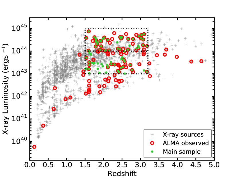
Figure 1: X-ray luminosity (2-10 keV: rest frame) versus redshift for the X-ray sources in the CDF-S and COSMOS fields. The X-ray sources that lie within our ALMA observations are indicated as red circles (see appendix). The X-ray AGN used in our star formation analyses, which comprise our main sample, are further highlighted with green filled circles (see §2.1); the dotted square indicates the region of the X-ray luminosity–redshift plane used in our main analyses. Not all of the objects in the dotted square are selected for our main sample since many lie below our stellar mass threshold.

Overall our main sample includes 81 X-ray AGN. In Figure 1 we plot the X-ray luminosity versus redshift of the overall X-ray source population in the CDF-S and COSMOS fields and highlight the $z$–$L_{\rm X}$ parameter space explored by our main sample. The properties of the individual X-ray AGN in the main sample are presented in Tables 1 and 2. Of the 81 X-ray AGN, 63 ($\approx$ 78%) have SFR measurements or upper limits augmented by ALMA observations. To search for trends in the star forming properties of X-ray AGN as a function of key properties, we also defined subsamples based on X-ray luminosity and stellar mass: low $L_{\rm X}$ ($10^{43}-10^{44}\mathrel{\rm erg\;s^{-1}}$; 39 X-ray AGN), high $L_{\rm X}$ ($10^{44}-10^{45}\mathrel{\rm erg\;s^{-1}}$; 42 X-ray AGN), low mass ($2\times 10^{10}-8\times 10^{10}\mathrel{\rm M_{\odot}}$; 41 X-ray AGN), and high mass ($8\times 10^{10}-1\times 10^{12}\mathrel{\rm M_{\odot}}$; 40 X-ray AGN). We note that the mean and median redshifts of the $L_{\rm X}$ and stellar mass subsamples are well matched: $\delta z=$ 0.1 for the $L_{\rm X}$ subsamples and $\delta z=$ 0.05 for the stellar mass subsamples.

2.1.1 Stellar mass measurements

The stellar masses of the X-ray AGN were calculated by performing SED fitting on the broad-band UV-MIR photometry ($0.1$–$24$ $\mu$m) from archival catalogs in the CDF-S and COSMOS fields. For the sources in the CDF-S field, we used the multi-wavelength catalogue of Guo et al. (2013), which covers the CANDELS GOODS-S Deep+Wide+ERS area. A fraction ($\approx$ 33%) of our targets lie outside the CANDELS footprint; for these, we included photometry from the MUSYC ECDFS catalog of Cardamone et al. (2010). For the sources in the COSMOS field, we used the multi-wavelength catalogue of Laigle et al. (2016). Catalogue-specific procedures were used to convert tabulated aperture photometry to zero-point corrected total photometry. In both fields, we used Spitzer MIPS 24 $\mu$m photometry from Le Floc’h et al. (2009) and the PEP survey (Lutz et al., 2011) to extend the SEDs into the observed MIR.

We modelled the broad-band SEDs of the X-ray AGN using the CIGALE package (v0.8.1, Burgarella et al., 2005; Ciesla et al., 2015). The SEDs were fitted using combinations of stellar and AGN emission templates. The population synthesis models of Bruzual & Charlot (2003) represented the stellar emission, to which dust extinction was applied following the power-law prescription of Charlot & Fall (2000). The AGN emission was modelled on the library of Fritz et al. (2006), which takes a fixed shape power-law SED representing an accretion disc, and geometry-dependent dust emission from a smooth AGN torus. After an examination of the entire Fritz et al. (2006) library, we adopted a subset of the AGN templates (described below) that reproduce empirical AGN IR SEDs (e.g.; Mullaney et al., 2011; Mor & Netzer, 2012). We fixed the power-law indices that describe the radial and polar dust density distribution in the torus to 0.0 and 6.0, implying a uniform density torus that has a sharp gradient with elevation. We assumed a single value of 150.0 for the ratio between the outer radius and inner (sublimation) radius of the torus, and allowed for three values of the 9.7 $\mu$m Si optical depth (0.1, 1.0, 3.0). We allowed for the full range in torus inclination angles with respect to the line of sight and set the normalisation of the torus models to run through the MIPS 24 $\mu$m photometric point.

From the posterior distributions of stellar mass for each galaxy computed using CIGALE, we calculated the median stellar mass and the 16^th and 84^th percentile values as a measure of the uncertainty on the stellar mass; see Tables 1 & 2.

2.1.2 Star-formation measurements

The star forming properties of the X-ray AGN were calculated from Spitzer-IRAC $8\mu$m, Spitzer-IRS $16\mu$m, Spitzer-MIPS $24\mu$m, deblended Herschel-PACS (70, 100, 160 $\mu$m), deblended Herschel-SPIRE (250, 350, 500 $\mu$m) and our ALMA photometry ($870\mu$m, see appendix for more details). The Spitzer and Herschel photometry were taken from the same catalogues as for our earlier Stanley et al. (2015) study: the Spitzer IRAC and IRS data is from Sanders et al. (2007), Damen et al. (2011) and Teplitz et al. (2011) for the CDF-S, COSMOS, and GOODS-S fields, respectively. The deblended photometry consists of the MIPS $24\mu$m and the PACS bands from Magnelli et al. (2013) and SPIRE photometry from Swinbank et al. (2014). For the objects that were undetected in the Spitzer and Herschel maps, we calculated $3\sigma$ upper limits.

We used SED decomposition techniques to separate the AGN and star-forming components from the total IR SED. The full SED fitting procedure is presented in Stanley et al. (submitted); however, we provide brief details here and note that we used a slightly modified approach to obtain the final SFR values and errors for application in our sSFR distribution fitting (see §2.2). The SED fitting procedure is based on Stanley et al. (2015), which fitted AGN and star forming templates to Spitzer and Herschel photometry but is updated to include ALMA continuum measurements. The AGN and 5 of the 6 star forming templates are from Mullaney et al. (2011) but extrapolated to $3-1000\mu$m by Del Moro et al. (2013), while a $6^{\rm th}$ star forming template is the Arp220 galaxy template from Silva et al. (1998), which represents an extremely dusty star forming galaxy. The photometric measurements, uncertainties, and upper limits were taken into account when fitting the IR SEDs. Two sets of best-fitting SED solutions were calculated for each X-ray AGN, giving 12 best-fitting SED solutions overall: one set using each of the 6 star forming templates and the other set using the 6 star forming templates plus the AGN template. To determine whether the fit requires an AGN component or not, we used the Bayesian Information Criteria (BIC; Schwarz, G, 1978) which allows for an objective comparison between non-nested models with a fixed data set (see section 2.3.2). To establish if the fit of the source requires an AGN component, the SED with the AGN component has to have a smaller BIC than that of the SED with no AGN component with a difference of $\Delta$BIC>2 (for more information and examples see §3 of Stanley et al., submitted). This way we obtain 6 SED solutions.

We integrated each star forming template from each of the 6 SED solutions to estimate the total IR luminosities due to star formation for that SED solution ($\mathrel{\rm L_{IR,SF,Sol}}$). Using this procedure we obtained 6 different values of $\mathrel{\rm L_{IR,SF,Sol}}$ and their errors from the fitting routine. The final value of the IR luminosity due to star formation ($\mathrel{\rm L_{IR,SF}}$) and its error is calculated using the Bootstrap method. To each value of $\mathrel{\rm L_{IR,SF,Sol}}$ we assigned a probability P($\chi^{2}$) (in the shape of the $\chi^{2}$ distribution) that it is the true value of $\mathrel{\rm L_{IR,SF}}$. Then we picked a $\mathrel{\rm L_{IR,SF,Sol}}$ based on its P($\chi^{2}$) and drew a value of $\mathrel{\rm L_{IR,SF}}$ from a normal distribution with the mean and width as the best value and error returned from $\mathrel{\rm L_{IR,SF,Sol}}$. We repeated this procedure $10^{5}$ times to build a distribution of all possible values of $\mathrel{\rm L_{IR,SF}}$. The created distribution was dominated by the template with the least $\chi^{2}$ value, but it also took into consideration other template solutions. For the upper limit calculations, we selected an SED solution with the highest value of $\mathrel{\rm L_{IR,SF,Sol}}$.

We converted $\mathrel{\rm L_{IR,SF}}$ to SFR using Equation 4 from Kennicutt (1998) corrected to the Chabrier (2003) IMF. In order to calculate the sSFR we also created a distribution of stellar masses for each object by drawing $10^{5}$ times from the normal distribution with the mean and width as the best value and error returned from CIGALE (see §2.1.1). We then calculated the sSFR by dividing draws of SFR by the draws of stellar mass. We calculated the final (and adopted) values of the SFR and sSFR and their errors as the median and standard deviation of the $10^{5}$ SFR and sSFR values, respectively; see Tables 1 & 2.

With ALMA photometry the fraction of AGN with SFR measurement increased for the low and high $L_{\rm X}$ subsamples from $7\%$ and $17\%$ to $31\%$ and $38\%$, respectively (described in detail in Stanley et al, submitted). Also for those objects which remained with a SFR upper limit even with ALMA photometry, the SFR upper limits have decreased by up to factor of $10$ (Stanley et al, submitted). This significantly increased detection fraction and improved upper limits allows us to estimate the specific star-formation distributions, which was not possible without the ALMA data (see §2.2).

Table 1: X-ray selected AGN in the main sample from the CDF-S field. The columns show the X-ray ID, optical position, redshift (2 and 3 decimal places indicate photometric and spectroscopic redshifts, respectively), X-ray luminosity (rest-frame 2-10 keV) (all from Hsu et al., 2014), the estimated SFR from our IR SED fitting (see §2.1.2, the estimated stellar mass from our UV–MIR SED fitting (see §2.1.1), and a flag to indicate whether the X-ray AGN was observed with ALMA (see Table A1).

X-ray ID	RA	Dec	Redshift	log10	log10	log10	Observed
	(J2000)	(J2000)		(L2-10keV/erg s-1)	(SFR/M⊙yr${}^{-1})$	(M∗/M⊙)	with ALMA?
88	$53.01025$	$-27.76681$	$1.616$	$43.5$	$2.30\pm 0.04$	$10.99\pm 0.19$	yes
93	$53.01271$	$-27.74731$	$2.573$	$43.5$	$<1.81$	$10.97\pm 0.21$	yes
111	$53.02229$	$-27.77890$	$2.51$	$43.7$	$1.83\pm 0.04$	$11.28\pm 0.23$	no
117	$53.02548$	$-27.82436$	$1.69$	$43.5$	$1.83\pm 0.16$	$10.97\pm 0.15$	no
142	$53.03637$	$-27.66547$	$1.54$	$43.2$	$1.69\pm 0.18$	$10.84\pm 0.21$	no
166	$53.04548$	$-27.73749$	$1.615$	$43.9$	$2.27\pm 0.02$	$10.46\pm 0.17$	no
176	$53.04905$	$-27.77449$	$1.51$	$43.2$	$2.03\pm 0.04$	$10.35\pm 0.15$	no
188	$53.05392$	$-27.87690$	$2.562$	$44.0$	$<1.81$	$10.49\pm 0.21$	no
199	$53.05791$	$-27.83357$	$2.42$	$43.1$	$<2.25$	$11.40\pm 0.16$	yes
211	$53.06195$	$-27.85111$	$1.60$	$43.2$	$1.71\pm 0.17$	$10.71\pm 0.15$	yes
213	$53.06240$	$-27.70691$	$1.891$	$43.0$	$<2.20$	$11.79\pm 0.16$	no
215	$53.06331$	$-27.69971$	$2.402$	$43.1$	$<1.68$	$10.86\pm 0.23$	yes
222	$53.06595$	$-27.70185$	$2.07$	$43.1$	$<1.69$	$11.10\pm 0.23$	no
240	$53.07128$	$-27.69358$	$2.20$	$43.5$	$<2.21$	$10.81\pm 0.22$	no
257	$53.07645$	$-27.84873$	$1.536$	$43.7$	$<2.07$	$11.17\pm 0.23$	yes
277	$53.08318$	$-27.71205$	$2.21$	$43.4$	$<2.20$	$10.45\pm 0.23$	yes
290	$53.08738$	$-27.92962$	$2.54$	$43.6$	$<1.49$	$11.04\pm 0.24$	yes
301	$53.09235$	$-27.80322$	$2.47$	$43.2$	$<2.41$	$10.92\pm 0.22$	yes
310	$53.09408$	$-27.80419$	$2.39$	$43.1$	$<1.64$	$10.68\pm 0.23$	yes
344	$53.10491$	$-27.70528$	$1.617$	$43.4$	$<1.76$	$11.22\pm 0.15$	yes
359	$53.10816$	$-27.75405$	$2.728$	$43.4$	$1.84\pm 0.07$	$10.56\pm 0.18$	yes
369	$53.11110$	$-27.67038$	$1.658$	$43.8$	$1.65\pm 0.08$	$10.49\pm 0.22$	no
410	$53.12414$	$-27.89127$	$2.53$	$43.3$	$2.24\pm 0.12$	$11.13\pm 0.17$	yes
440	$53.13244$	$-27.95390$	$2.10$	$43.4$	$<2.10$	$10.68\pm 0.20$	no
443	$53.13366$	$-27.69865$	$1.982$	$43.3$	$<1.85$	$10.83\pm 0.20$	no
450	$53.13639$	$-27.86421$	$1.95$	$43.4$	$<1.92$	$11.24\pm 0.17$	no
456	$53.13805$	$-27.86831$	$3.17$	$43.1$	$<1.84$	$10.68\pm 0.23$	yes
466	$53.14169$	$-27.81662$	$2.78$	$43.2$	$<1.87$	$10.73\pm 0.19$	yes
486	$53.14670$	$-27.88834$	$1.84$	$43.5$	$2.19\pm 0.03$	$10.41\pm 0.21$	no
490	$53.14883$	$-27.82112$	$2.578$	$43.0$	$<1.77$	$11.24\pm 0.24$	no
522	$53.15850$	$-27.77403$	$2.12$	$43.3$	$<1.83$	$10.38\pm 0.24$	yes
524	$53.15959$	$-27.93142$	$3.10$	$43.1$	$2.69\pm 0.04$	$11.49\pm 0.21$	no
549	$53.16557$	$-27.76979$	$1.754$	$43.5$	$<2.54$	$10.81\pm 0.22$	no
575	$53.17935$	$-27.81251$	$1.730$	$43.4$	$<2.03$	$10.75\pm 0.18$	no
620	$53.19608$	$-27.89264$	$2.48$	$43.7$	$<1.72$	$10.86\pm 0.20$	no
625	$53.19886$	$-27.84391$	$1.615$	$43.0$	$<2.20$	$11.06\pm 0.18$	no
633	$53.20492$	$-27.91801$	$2.30$	$43.4$	$2.15\pm 0.02$	$10.59\pm 0.20$	yes
663	$53.22878$	$-27.75165$	$1.84$	$43.2$	$<1.85$	$11.21\pm 0.24$	no
683	$53.24718$	$-27.81631$	$1.65$	$43.9$	$<2.13$	$11.35\pm 0.18$	no

Table 2: X-ray selected AGN in our main sample from the COSMOS field. The columns show the X-ray ID, optical position, redshift (2 and 3 decimal places indicate photometric and spectroscopic redshifts, respectively), X-ray luminosity (rest-frame 2-10 keV) (all from Marchesi et al., 2016), SFR from our IR SED fitting (see §2.1.2), stellar mass from our UV–MIR SED fitting (see §2.1.1), and a flag to indicate whether the X-ray AGN was observed with ALMA (see Table A2).

X-ray ID	RA	Dec	Redshift	log10	log10	log10	Observed
	(J2000)	(J2000)		(L2-10keV/erg s-1)	(SFR/M⊙yr${}^{-1})$	(M∗/M⊙)	with ALMA?
cid $434$	$149.72072$	$2.34901$	$1.530$	$44.6$	$<1.63$	$11.70\pm 0.18$	yes
cid $580$	$149.85469$	$2.60694$	$2.11$	$44.5$	$<1.81$	$11.13\pm 0.22$	yes
cid $558$	$149.88252$	$2.50513$	$3.10$	$44.8$	$1.53\pm 0.18$	$11.42\pm 0.21$	yes
cid $330$	$149.95583$	$2.02806$	$1.753$	$44.6$	$<1.65$	$10.72\pm 0.26$	yes
cid $2177$	$149.96660$	$2.43247$	$2.89$	$44.1$	$1.63\pm 0.07$	$11.20\pm 0.23$	no
cid $529$	$149.98158$	$2.31501$	$3.017$	$44.6$	$<1.80$	$11.43\pm 0.20$	yes
cid $474$	$149.99390$	$2.30146$	$1.796$	$44.5$	$1.11\pm 0.27$	$10.38\pm 0.20$	yes
cid $451$	$150.00253$	$2.25863$	$2.450$	$44.6$	$1.14\pm 0.19$	$11.19\pm 0.19$	yes
cid $1127$	$150.01057$	$2.26939$	$2.390$	$44.1$	$<1.49$	$11.02\pm 0.19$	yes
cid $532$	$150.01985$	$2.34914$	$1.796$	$44.4$	$<1.82$	$11.49\pm 0.23$	yes
cid $1216$	$150.02008$	$2.35365$	$2.663$	$44.1$	$<1.86$	$10.69\pm 0.20$	yes
cid $659$	$150.03290$	$2.45859$	$2.045$	$44.0$	$1.29\pm 0.12$	$10.89\pm 0.19$	yes
cid $1214$	$150.03677$	$2.35852$	$1.59$	$44.0$	$<1.62$	$10.97\pm 0.21$	yes
cid $351$	$150.04262$	$2.06329$	$2.018$	$44.6$	$<1.62$	$11.15\pm 0.15$	yes
cid $443$	$150.04597$	$2.20114$	$2.704$	$44.2$	$<1.81$	$10.95\pm 0.18$	no
cid $458$	$150.05524$	$2.14317$	$1.974$	$44.5$	$1.27\pm 0.18$	$10.83\pm 0.25$	no
cid $352$	$150.05891$	$2.01518$	$2.498$	$44.6$	$1.41\pm 0.04$	$10.83\pm 0.23$	yes
cid $1215$	$150.06454$	$2.32905$	$2.450$	$44.1$	$<1.46$	$11.00\pm 0.24$	yes
cid $72$	$150.09154$	$2.39908$	$2.475$	$44.6$	$<1.85$	$10.99\pm 0.22$	yes
cid $466$	$150.10094$	$2.16782$	$2.055$	$44.0$	$<1.44$	$10.75\pm 0.17$	no
cid $149$	$150.10371$	$2.66577$	$2.955$	$44.7$	$<1.83$	$11.06\pm 0.27$	yes
cid $1144$	$150.10477$	$2.24364$	$1.912$	$44.1$	$<1.64$	$10.86\pm 0.24$	yes
cid $86$	$150.11958$	$2.29591$	$1.831$	$44.3$	$<1.46$	$11.40\pm 0.18$	yes
cid $87$	$150.13304$	$2.30328$	$1.598$	$44.9$	$1.53\pm 0.18$	$11.52\pm 0.22$	yes
cid $965$	$150.15218$	$2.30785$	$3.178$	$44.2$	$1.41\pm 0.19$	$10.83\pm 0.17$	yes
cid $914$	$150.18001$	$2.23128$	$2.146$	$44.0$	$1.60\pm 0.18$	$10.90\pm 0.17$	yes
cid $124$	$150.20532$	$2.50293$	$3.07$	$44.3$	$<1.80$	$10.79\pm 0.16$	yes
cid $83$	$150.21416$	$2.47502$	$3.075$	$44.5$	$<1.83$	$11.21\pm 0.20$	yes
cid $21$	$150.21466$	$2.20428$	$1.841$	$44.4$	$1.50\pm 0.22$	$10.41\pm 0.30$	no
cid $23$	$150.22403$	$2.27080$	$2.944$	$44.2$	$1.26\pm 0.24$	$11.88\pm 0.19$	no
cid $127$	$150.22702$	$2.53761$	$1.801$	$44.4$	$2.08\pm 0.08$	$11.12\pm 0.23$	no
cid $954$	$150.23180$	$2.36401$	$1.936$	$44.2$	$<1.83$	$10.64\pm 0.30$	yes
cid $970$	$150.23550$	$2.36176$	$2.501$	$44.6$	$<2.20$	$11.30\pm 0.17$	yes
cid $75$	$150.24779$	$2.44215$	$3.029$	$44.7$	$2.73\pm 0.05$	$10.87\pm 0.20$	yes
cid $725$	$150.27097$	$2.36507$	$2.962$	$44.2$	$<2.42$	$10.73\pm 0.16$	no
cid $89$	$150.28117$	$2.41590$	$2.372$	$44.4$	$2.69\pm 0.05$	$10.69\pm 0.22$	no
cid $90$	$150.28482$	$2.39505$	$1.932$	$44.4$	$<2.11$	$11.29\pm 0.25$	yes
cid $365$	$150.28563$	$2.01459$	$2.671$	$44.5$	$<2.55$	$10.62\pm 0.20$	yes
cid $94$	$150.30956$	$2.39915$	$1.802$	$44.6$	$<2.26$	$11.01\pm 0.18$	no
cid $58$	$150.32689$	$2.09415$	$2.798$	$44.5$	$<2.41$	$11.89\pm 0.23$	yes
cid $53$	$150.34372$	$2.14067$	$1.787$	$44.2$	$2.48\pm 0.06$	$11.09\pm 0.20$	yes
cid $62$	$150.37364$	$2.11203$	$1.914$	$44.5$	$<2.48$	$10.51\pm 0.30$	yes

2.2 Measuring the (specific) star-formation distributions

The majority of previous studies have explored the mean SFRs and sSFRs of X-ray AGN. However, the mean is sensitive to bright outliers and can hide subtle trends in the data. A more comprehensive approach to characterising the star forming properties of X-ray AGN, is the measurement of the distributions of SFRs and sSFRs. In our analyses here we fitted the SFR and sSFR distributions of the X-ray AGN assuming a log-normal function:

$$N(x)\propto\exp\left(-\frac{\log_{10}\left(\frac{x}{\mu}\right)^{2}}{2w^{2}}\right),$$ (1)

where $x$ is the SFR or sSFR, $\mu$ is the mode, and $w$ is the width of the distribution. The motivation for fitting a log-normal function is: 1) the SFR and sSFR values for main-sequence galaxies broadly follow this distribution (e.g. Schreiber et al., 2015), and 2) the SFR and sSFR distributions of the AGN in the EAGLE simulations are consistent with a log-normal function, as we demonstrate in §3.1. Also, our source statistics are not high enough to fit a more complex model with more parameters. However, even if the log-normal distribution is not absolutely correct, it allows us to broadly characterise the typical values and range in values to search for trends and compare to the different models (see §4.2).

The majority ($\approx$ 65 %) of the X-ray AGN in our main sample are undetected by both Herschel and ALMA and therefore only have a SFR upper limit. The SFR and sSFR distributions cannot be obtained trivially without the appropriate consideration of these limits. Following Mullaney et al. (2015), we use a hierarchical Bayesian method to find the best fitting parameters to sample the probability distribution (PD) of our parameters $\mu$ and $w$, using Gibbs sampling and Metropolis-Hastings Markov Chain Monte Carlo (MCMC) algorithms. There are several advantages of this method: 1) the uncertainties and upper limits can be taken into account, and 2) the PD produced in this way can be used to estimate errors on $\mu$ and $w$. The fitting routine treats upper limits and detections differently, but in a statistically consistent way. For a detection, we assumed that the likelihood function of the errors has a log-normal shape, while for the upper limits we assumed that the likelihood function is in the form of a log-error function. The final values and errors of the mode $\mu$ and width $w$ are taken to be the median values of the PD and the $68\%$ confidence interval, respectively. As was done in Mullaney et al. (2015), we assume uniform, uninformative priors on $\mu$ and $w$ which do not influence the final PDs. We quote the final values of our fits to the sSFR distributions for the main sample (see §3.1) in Table 3.

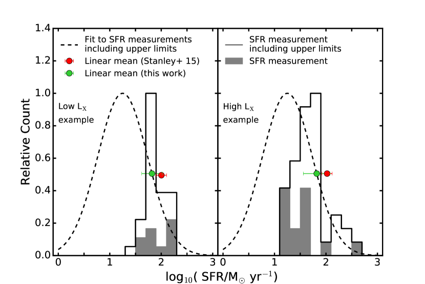
Figure 2: Example SFR distributions to demonstrate our model-fitting approach; see §2.2. The X-ray AGN lie at $z=$ 1.5–2.5 and have L${}_{X}=10^{43}-10^{44}\mathrel{\rm erg\;s^{-1}}$ (left panel) and L${}_{X}=10^{44}-10^{45}\mathrel{\rm erg\;s^{-1}}$ (right panel). The filled grey histogram indicates the distribution of SFR measurements and the unfilled histogram indicates the distribution of SFR measurements including upper limits. The dashed curve indicates the best-fitting log-normal distribution to the measured SFRs including upper limits (see §2.2) and the filled green circle indicates the mean SFR calculated from the best-fitting distribution. The filled red circle indicates the mean SFR from Stanley et al. (2015) for a larger sample of X-ray AGN at $z=$1.5–2.5 in the same $L_{\rm X}$ range but with SFR constraints from Spitzer and Herschel data. The error bars represent the $68\%$ confidence interval for each of the measurements.

We now test whether our method and data are consistent with earlier work, in particular Stanley et al. (2015), which used the same SED-fitting code as that adopted in this study. This earlier study relied on calculating linear means of SFR and stacking and therefore only presented linear means in bins of $L_{\rm X}$, with no differentiation of the sample by stellar mass. Therefore, to replicate this study in the limited range of redshift and $L_{\rm X}$ of our sample, we calculate the linear means of SFR of all AGN (including those with $\rm M_{*}<2\times 10^{10}\mathrel{\rm M_{\odot}}$) in the $z=1.5-2.5$ redshift range. This was done directly from the corresponding log-normal distributions as follows:

$$\langle x\rangle=10^{(\mu+1.15w^{2})},$$ (2)

where $\mu$ is the mode and $w$ is the width of the distribution as in Equation 1. The linear mean was calculated from the PD of $\mu$ and $w$ from our MCMC analysis, from which the median and $68\%$ confidence interval were derived.

The $\log_{10}(\mathrel{\langle\rm SFR\rangle}/\mathrel{\rm M_{\odot}yr^{-1}})$ of our low and high $L_{\rm X}$ subsamples were $1.94^{+0.33}_{-0.20}$ and $1.8^{+0.22}_{-0.15}$, respectively, as compared to $2.00\pm 0.10$ and $2.02\pm 0.10$ from Stanley et al. (2015), see Figure 2. As such, our estimates are in good agreement with those of Stanley et al. (2015) and confirms that our new method is consistent with previous work. In comparison, the $\log_{10}(\mu/\mathrel{\rm M_{\odot}yr^{-1}})$ of the SFR distribution for low and high $L_{\rm X}$ subsamples are $1.27^{+0.31}_{-0.22}$ and $1.12^{+0.15}_{-0.19}$, respectively. The linear mean of the SFR is always higher (depending on the width of the distribution) than the mode of the distribution, making the mode of the distribution a more reliable tracer of the typical values of the population. In summary, our method yields consistent result with previous studies using linear means and stacking procedures.

Table 3: Best fitting log-normal fit parameters for the sSFR distributions of our main sample and sample from EAGLE simulations binned by X-ray luminosity and stellar mass. The quoted $\mu$ and $w$ and their errors are the median of the their posterior probability distributions (PDs) and $68\%$ confidence intervals. The linear mean is calculated from $\mu$ and $w$ using equation 2.

Sample	Mode ($\mu$)	Width($w$)	linear mean
	$\log_{10}(\mu$/Gyr-1)	(dex)	$\log_{10}(\mathrel{\langle\rm sSFR\rangle}$/Gyr-1)
Main Sample (Observed AGN):
Low $L_{x}$ AGN	$0.03^{+0.14}_{-0.17}$	$0.52^{+0.13}_{-0.10}$	$0.34^{+0.18}_{-0.15}$
High $L_{x}$ AGN	$-0.32^{+0.15}_{-0.17}$	$0.65^{+0.15}_{-0.11}$	$0.17^{+0.26}_{-0.19}$
Low Mass AGN	$-0.01^{+0.13}_{-0.15}$	$0.53^{+0.13}_{-0.08}$	$0.31^{+0.16}_{-0.14}$
High Mass AGN	$-0.48^{+0.17}_{-0.20}$	$0.67^{+0.18}_{-0.12}$	$0.05^{+0.29}_{-0.22}$
EAGLE ref model:
Low $L_{x}$ AGN	$-0.08^{+0.05}_{-0.04}$	$0.45^{+0.06}_{-0.06}$	$0.14^{+0.08}_{-0.1}$
High $L_{x}$ AGN	$0.14^{+0.05}_{-0.04}$	$0.45^{+0.05}_{-0.04}$	$0.38^{+0.08}_{-0.07}$
Low Mass AGN	$0.04^{+0.02}_{-0.02}$	$0.47^{+0.02}_{-0.02}$	$0.23^{+0.03}_{-0.03}$
High Mass AGN	$-0.23^{+0.07}_{-0.07}$	$0.42^{+0.05}_{-0.05}$	$-0.03^{+0.09}_{-0.07}$
Low Mass galaxy	$-0.14^{+0.02}_{-0.02}$	$0.48^{+0.02}_{-0.02}$	$0.22^{+0.02}_{-0.02}$
High Mass galaxy	$-0.31^{+0.02}_{-0.02}$	$0.45^{+0.02}_{-0.02}$	$-0.15^{+0.02}_{-0.02}$
EAGLE no AGN model:
Low Mass galaxy	$0.13^{+0.01}_{-0.01}$	$0.23^{+0.01}_{-0.01}$	$0.20^{+0.02}_{-0.02}$
High Mass galaxy	$-0.10^{+0.01}_{-0.01}$	$0.28^{+0.01}_{-0.01}$	$0.0^{+0.02}_{-0.02}$

2.3 EAGLE hydrodynamical simulation and source properties

Cosmological simulations of galaxy formation have provided some of the most compelling evidence that AGN feedback has a significant effect on star formation in the galaxy population. To aid in the interpretation of our data we have therefore compared the sSFR distributions of the X-ray AGN in our main sample to those computed from the EAGLE cosmological hydrodynamical simulation (Crain et al., 2015; Schaye et al., 2015). A key advantage of our approach is that we can compare our results to models from the cosmological simulations both with and without AGN feedback included, to allow us to identify the signature of AGN feedback on the star forming properties of galaxies (also see e.g. Beckmann et al., 2017; Harrison, 2017).

EAGLE is a suite of cosmological hydrodynamical simulations, which uses an enhanced version of the GADGET-3 code (Springel, 2005) which consists of a modified hydrodynamics solver, time-step limiter, and employs a subgrid treatment of baryonic physics. The subgrid physics takes into account of the stellar-mass loss, element-by-element radiative cooling, star formation, black-hole accretion (i.e., AGN activity), and star formation and AGN feedback. The free parameters of the subgrid physics were calibrated on the stellar mass function, galaxy size, and the black-hole–spheroid relationships at $z\approx 0.1$ (Crain et al., 2015; Schaye et al., 2015). The simulation is able to reproduce a wide range of observations of low and high redshift galaxies (e.g., fraction of passive galaxies, Tully-Fisher relation, evolving galaxy stellar mass function, galaxy colours and the relationship between black hole accretion rates and SFRs; see e.g. Furlong et al., 2015; Schaye et al., 2015; McAlpine et al., 2017; Trayford et al., 2017). We note that, AGN feedback was introduced in the EAGLE reference model to reduce the star-formation efficiency of the most massive galaxies in order to reproduce the turn-over at the high mass end of the local galaxy stellar mass function (Crain et al., 2015). The model also effectively re-produces the bi-modality of colours of local galaxies (see Trayford et al., 2015). However; although related, the EAGLE reference model was not directly calibrated on the parameters of the SFR or sSFR distributions at multiple epochs, making our comparison with these observables an independent test of the model.

In our analyses we have used two models from EAGLE: the reference model (hereafter EAGLE ref), designed to reproduce a variety of key observational properties (see above), and a model with no AGN feedback (hereafter EAGLE noAGN). The EAGLE noAGN model is identical to the EAGLE ref model in all aspects except black holes are not seeded, which effectively turns off the AGN feedback. A comparison of the results between these two models therefore allows for the identification of the signature of AGN feedback on the star forming properties of the simulated galaxies. The EAGLE ref model was run at volumes of $25^{3}$, $50^{3}$, and $100^{3}$ cubic comoving megaparsecs (cMpc³). We present here the results from the largest volume which contains the largest number of rare high-mass systems; however, we note that we performed our analysis on all volumes and found no significant differences in the overall results. The EAGLE noAGN model was only performed at a volume of $50^{3}$ cubic comoving megaparsecs. A summary of the two different EAGLE models used in our analyses are given in Table 4.

Table 4: Basic properties of the EAGLE models used in the paper. From left to right: the model name used in the text, the reference name in the EAGLE database, the comoving volume (cMpc³), the initial mass m_g of the baryonic particles, and a flag to indicate whether AGN feedback was adopted in the model. See Schaye et al. (2015) for more information.

Model name	Database	Volume	mg	AGN
in text	Reference	(cMpc3)	(M⊙)	feedback?
EAGLE ref	RefL0100N1504	$100^{3}$	$1.81\times 10^{6}$	Yes
EAGLE no AGN	NoAGNL0050N0752	$50^{3}$	$1.81\times 10^{6}$	No

In order to construct the AGN and galaxy catalogues from the EAGLE models we queried the public database (McAlpine et al., 2016) for any dark matter halo with a galaxy of stellar mass of $M_{*}>2\times 10^{10}\mathrel{\rm M_{\odot}}$, for redshift snapshots over $z=$ 1.4–3.6; the slightly broader redshift range than that adopted for our main sample ensures that the AGN and galaxy samples from EAGLE have the same mean and median redshift as our main sample. We then applied the same stellar mass and AGN luminosity cuts to the EAGLE sample as we used to select our main sample. To calculate the properties of the simulated AGN and galaxies, to allow for a systematic comparison to our main sample, we also: 1) converted the black-hole accretion rates from the EAGLE ref model to $L_{\rm X}$ by converting them first to AGN bolometric luminosities (assuming a nominal radiative efficiency of $\epsilon=10\%$) and then converting to $L_{\rm X}$ by multiplying it by a bolometric correction factor of $0.1$ (McAlpine et al., 2017) and 2) scaled up the SFRs calculated in both EAGLE models by $0.2$ dex to account for the offset found by Furlong et al. (2015) (see also §2.4 of McAlpine et al. 2017) from comparing the global SFR density of the EAGLE ref model to the observed global SFR density of galaxies. Therefore, the overall galaxy population had the same selection criteria as the AGN, but we did not apply any $L_{\rm X}$ threshold. The galaxies include both active and inactive galaxies as well as star-forming and passive galaxies. In total we found $472$ AGN and $2333$ galaxies in the EAGLE ref model and $682$ galaxies in the EAGLE noAGN model with the same properties as in our main sample.

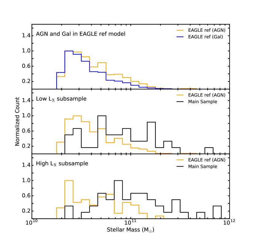
Figure 3: Comparison of the normalized stellar mass distributions from our different samples. Top panel: Comparison of the stellar mass distributions of the AGN in the EAGLE ref model (blue line) and galaxies in the EAGLE ref model (orange line). Middle Panel: Comparison of the stellar mass distribution of the low $L_{\rm X}$ AGN in the EAGLE ref model (orange line) and the low $L_{\rm X}$ AGN of the observed main sample (black line). Bottom panel: Comparison of the stellar mass distribution of the high $L_{\rm X}$ AGN in the EAGLE ref model (orange line) with the high $L_{\rm X}$ AGN of the main sample (black line). We take the differences in stellar mass distributions into consideration in §3.2.

We split the AGN in the EAGLE ref model into low and high $L_{\rm X}$ subsamples using the same luminosity threshold as for our main sample (see §2.1); the EAGLE ref low and high $L_{\rm X}$ subsamples contain 403 and 69 AGN, respectively. In Figure 3 we compare the stellar mass distributions of the simulated AGN and galaxies to the AGN in our main sample. The stellar mass distributions for the AGN in the EAGLE ref model and the main sample are different in both $L_{\rm X}$ subsamples. The median stellar masses of the low and high $L_{\rm X}$ AGN in the EAGLE ref model are both $10^{10.6}$ $\mathrel{\rm M_{\odot}}$. By comparison the median stellar masses of the observed low and high $L_{\rm X}$ subsamples in our main sample are $10^{10.7}$ and $10^{11.0}$ $\mathrel{\rm M_{\odot}}$, respectively. This difference in median stellar masses is caused by the different volumes probed to select the samples. While the EAGLE ref model has a volume of $10^{6}$ cMpc³, the low and high $L_{\rm X}$ subsamples of our main sample were selected from larger volumes of $10^{6.4}$ cMpc³ and $10^{7}$ cMpc³, respectively.

The differences in the stellar mass distributions between the AGN in the main sample and EAGLE will also cause the differences in the sSFR distributions (i.e. since the sSFR distributions also depend on stellar mass; see §3.1). We therefore have to take account of the different stellar mass distributions to fully compare the observed and simulated AGN. We do this using the mass matching methods described in §3.2.

3 Results

In this section we present our results on the sSFR distributions of the distant X-ray AGN in our main sample. We measure the sSFR distributions of our main sample and search for trends in the star forming properties as a function of $L_{\rm X}$ and stellar mass (see §3.1). To aid in the interpretation of our results we make comparisons to the EAGLE ref model (see §3.2).

3.1 sSFR trends with X-ray luminosity and stellar mass

To search for trends in the sSFR properties of the X-ray AGN, we measured the properties (i.e., the mode and the width) of the sSFR distributions as a function of $L_{\rm X}$ and stellar mass. The mode of the sSFR distribution provides a more reliable measurement of the typical sSFR than the linear mean (see Figure 2 and §2.2). The width of the sSFR distribution provides a basic measure of the range in sSFRs: a narrow width indicates that most systems have similar sSFRs while a broad width indicates a large range of sSFRs. We fitted log-normal distributions to the $L_{\rm X}$ and stellar mass subsamples within our main sample (see §2.1) using the method described in §2.2. Table 3 presents the overall results.

In Figure 4, we plot the sSFR properties (individual measurements and measurements of the distributions) of the main sample as a function of $L_{\rm X}$. The modes (log₁₀($\mu$/Gyr^-1)) of the sSFR distributions of the low $L_{\rm X}$ and high $L_{\rm X}$ subsamples are $0.03^{+0.14}_{-0.17}$ and $-0.32^{+0.15}_{-0.17}$, respectively. The mode of the sSFR decreases with $L_{\rm X}$, but the drop is modest ($1.5\sigma$), ruling out a simple AGN-feedback model where high-luminosity AGN instantaneously shut down SF. We also note that the same qualitative result is obtained if we consider the mean sSFR rather than the mode; however, the mean values are $\approx$ 0.3–0.5 dex higher than the mode (see Table 3). The widths of the sSFR distributions for the low $L_{\rm X}$ and high $L_{\rm X}$ subsamples are also consistent, with values of $0.52^{+0.13}_{-0.10}$ and $0.65^{+0.15}_{-0.11}$, respectively.

Our results shows no evolution of the sSFR distribution with $L_{\rm X}$. This general conclusion agrees qualitatively with results of most previous studies at these redshifts that investigated the mean (s)SFR as a function of $L_{\rm X}$ (Harrison et al., 2012; Rosario et al., 2012; Rovilos et al., 2012; Azadi et al., 2015; Stanley et al., 2015; Lanzuisi et al., 2017). Here, for the first time, we have constrained the sSFR distribution properties for the AGN host galaxies at these redshifts. These results demonstrate that the previous finding of a flat trend is a true reflection of the behaviour of the typical AGN population (as measured using the mode), rather than an inaccurate description of the population. However, as expected we showed that the bulk of the population (mode) has a lower sSFR than linear mean.

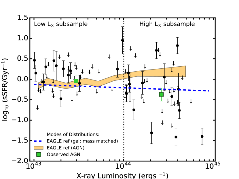
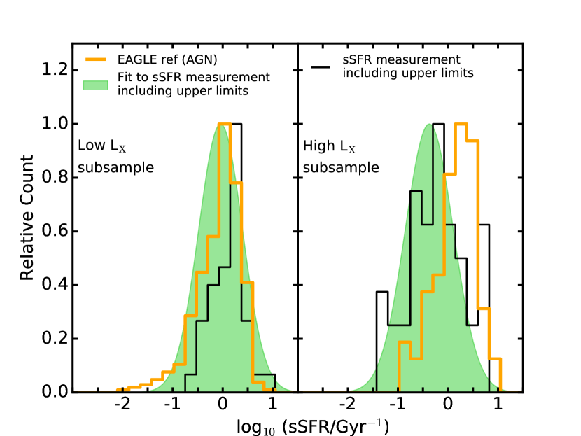
Figure 4: Top panel: sSFR versus X-ray luminosity (2–10 keV: rest frame) for the X-ray AGN in our main sample. The black filled circles indicate individual X-ray AGN, the filled green squares indicate the modes of the sSFR distributions for the low and high X-ray luminosity subsamples (see Table 3); error bars represent the $68\%$ confidence interval. The dotted vertical line indicates the division in X-ray luminosity between the low and high X-ray luminosity subsamples. The orange shaded region indicates the X-ray luminosity dependence on the sSFR distribution for AGN from the EAGLE ref model (the width corresponds to the $68\%$ confidence interval around the mode of the distribution) and the blue dashed line indicates the predicted sSFR–X-ray luminosity relationship from the EAGLE ref model for galaxies with masses matched to those found from our observed X-ray AGN (see §3.2). Bottom panel: sSFR distributions for our data (black histogram), the AGN from the EAGLE ref model (orange open histogram), and the best-fitting log-normal distribution (green filled histogram; see §2.2). The sSFR distributions are shown separately for the low (left) and high (right) X-ray luminosity subsamples.

In Figure 5, we plot the sSFR properties (individual measurements and measurements of the distributions) of the main sample as a function of stellar mass. Quantitatively similar results are obtained to those shown in Figure 4 for the sSFRs as a function of $L_{\rm X}$, with no clear evidence for a strong change in the sSFR properties towards high stellar mass: the mode (log₁₀($\mu$/Gyr^-1)) and width of the sSFR distribution for the low stellar mass subsample is $-0.01^{+0.13}_{-0.15}$ and $0.53^{+0.13}_{-0.08}$ respectively, while the mode (log₁₀($\mu$/Gyr^-1)) and width of the sSFR distribution for the high stellar mass subsample is $-0.48^{+0.17}_{-0.20}$ and $0.67^{+0.18}_{-0.12}$ respectively. However, the difference in the mode of the sSFR distributions between the two stellar mass subsamples is marginally more significant ($2.0\sigma$) than between the two $L_{\rm X}$ subsamples. Again, the mean sSFRs are also $\approx$ 0.3–0.5 dex higher than the modes (see Table 3). We put our results into context in section 4.1.

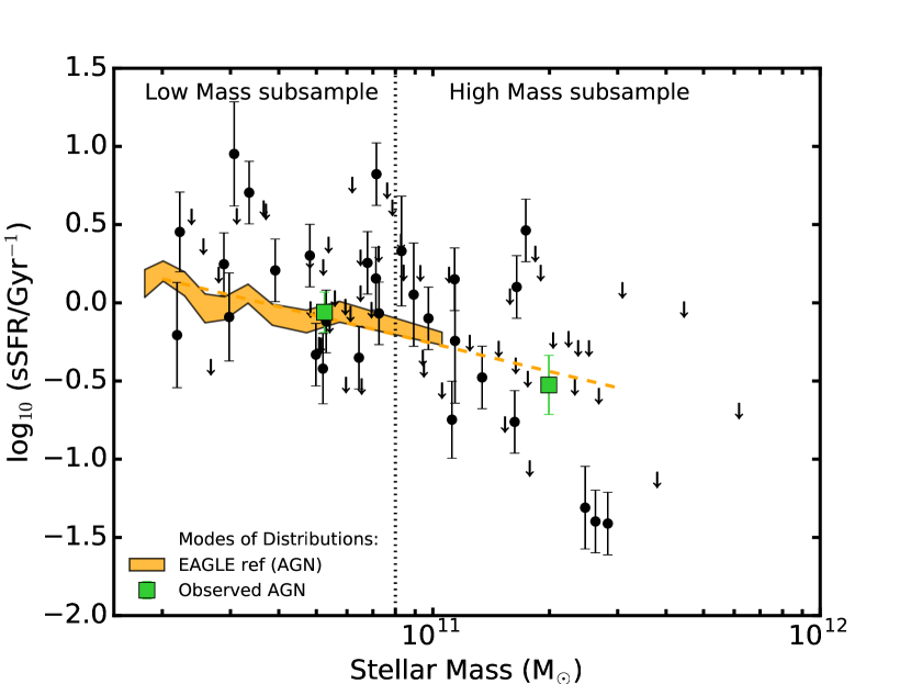
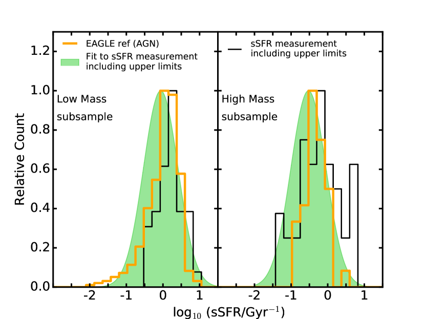
Figure 5: Top panel: sSFR versus stellar mass for the X-ray AGN in our main sample. The black filled circles indicate individual X-ray AGN, the filled green squares indicate the modes of the sSFR distributions for the low and high mass subsamples (see table 3); the error bars represent the $68\%$ confidence interval. The dotted vertical line indicates the division in mass between the low and high stellar mass subsamples. The orange shaded region indicates the stellar mass dependence on the sSFR distribution for AGN from the EAGLE ref model (the width corresponds to the $68\%$ confidence interval around the mode of the distribution) and the orange dashed line is the linear extrapolation of the mode to higher stellar masses (see §3.1). Bottom panel: sSFR distributions for our data (black histogram), the AGN from the EAGLE ref model (open orange histogram), and the best-fitting log-normal distribution (green filled histogram; see §2.2). The sSFR distributions are shown separately for the low (left) and high (right) stellar mass subsamples.

3.2 Comparison to the EAGLE simulations

The EAGLE ref model (see Table 4) reproduces the global properties of the galaxy population (see §2.3). To help interpret our results from §3.1, we investigate whether the simulated AGN in this model show the same sSFR relationships as we have found among the main sample we observed. The properties of the sSFR distributions are calculated for the EAGLE AGN in the same $L_{\rm X}$ and stellar-mass bins as for our main sample, following §2.2; see Table 3. To further aid in the comparison, we also calculated the running mode of the sSFR in $L_{\rm X}$ and stellar-mass bins of 50 objects, following §2.2.

In Figures 4 and 5, we compare the sSFR distributions of the EAGLE AGN to our main sample as a function of $L_{\rm X}$ and stellar mass, respectively. From these figures and Table 3, we note that EAGLE can generally reproduce the widths of the observed sSFR distributions of AGN. At low $L_{\rm X}$ and stellar mass, the modes of the sSFR distributions for the EAGLE AGN are also in good agreement with those of the main sample, but they deviate marginally at high stellar mass, and strongly at high $L_{\rm X}$.

We can qualitatively understand the marginal difference in the sSFR modes with stellar mass (see Figure 5) as due to the different stellar mass distributions between the simulated AGN in EAGLE and the observed AGN in the main sample. There are more massive AGN hosts in the main sample than in the EAGLE ref model, which is a consequence of the different volumes probed by the EAGLE simulation and our observational survey (see §2.3 and Figure 3). Since sSFR is a decreasing function of stellar mass, the more massive AGN in the main sample will have lower sSFRs than the less massive AGN. Indeed, if we extrapolate the running mode of the sSFR from the EAGLE ref model towards high stellar masses (the dashed line in Figure 5), we can fully reproduce the mode of the sSFR among the observed high mass AGN hosts.

Figure 3 shows that the stellar masses of the observed AGN and the simulated AGN from the EAGLE ref model differ substantially in the two $L_{\rm X}$ bins. This difference in stellar mass could also be the driver of the significant differences in the sSFR mode as a function of $L_{\rm X}$ seen between EAGLE and the main sample (see Figure 4). We explore this idea by considering how the mode of the sSFR changes for subsamples with different stellar mass distributions using the EAGLE ref model. Unfortunately, in the limited volume of the EAGLE simulation there are no AGN hosts with masses $>2\times 10^{11}$ M_⊙. Therefore, we turn to the more numerous galaxy population in the EAGLE ref model. So long as the sSFRs of these simulated galaxies decrease with stellar mass in the same functional form as the AGN, we can use them as analogues to understand the role of differing stellar mass distributions in the interpretation of the sSFR differences between the simulated and observed AGN. In Figure 6 we compare the mode of the sSFR distribution versus the stellar mass for both the AGN and galaxies in the EAGLE ref model and demonstrate that they follow the same trend but with a $\approx$ 0.1 dex offset (which we further explore in §4.1).

To quantify the impact of different stellar mass distributions on our results we constructed four subsets of galaxies from the EAGLE ref model that are matched in their mass distributions to 1) simulated AGN from the EAGLE ref model in the low $L_{\rm X}$ bin, 2) simulated AGN from the EAGLE ref model in the high $L_{\rm X}$ bin, 3) observed AGN from the main sample in the low $L_{\rm X}$ bin, and 4) observed AGN from the main sample in the high $L_{\rm X}$ bin. For each of these four subsets, we determined the mode of the sSFR distribution following the method in §2.2. If differences in stellar mass are the principal driver for the different trends shown by the observed and simulated AGN in Figure 4, we would expect offsets in the sSFR modes of the mass-matched subsets corresponding to the simulated and observed AGN in each respective $L_{\rm X}$ bin, particularly at high $L_{\rm X}$ where the stellar mass differences are most pronounced (see Figure 3). This is indeed what we find.

The mode of the sSFR for the two mass-matched EAGLE galaxy subsets corresponding to the low $L_{\rm X}$ bin differ by only a small amount ($<0.1$ dex), as expected given the similar stellar mass distributions (see Figure 3) and in agreement with the results for this $L_{\rm X}$ bin given in Table 3. On the other hand, the mode of the sSFRs for the two mass-matched EAGLE galaxy subsets corresponding to the high $L_{\rm X}$ bin differ by $\approx 0.4$ dex. From this we conclude that the high masses of the high $L_{\rm X}$ AGN in the main sample leads to a measured sSFR that is lower than that of equivalently X-ray luminous simulated AGN from the EAGLE ref model. If we correct the sSFR trend with $L_{\rm X}$ for the EAGLE AGN to reflect the different stellar mass distributions of the observed AGN, using the offsets determined above, we obtain the blue dashed line in Figure 4, which is a remarkably good match to our observations.

We have shown that even though EAGLE has not been calibrated on (s)SFR distributions of AGN, it reproduces accurately the shape and the parameters (mode and width) of the distribution. Furthermore, we have found that the properties of the sSFR distributions are more strongly related to stellar mass than to AGN luminosity. We investigated what these results mean in terms of AGN feedback in §4.2.

4 Discussion

On the basis of our results on the fitted sSFR distributions of X-ray AGN at $z=1.5-3.2$ we found that, once the effects of different volumes and survey selections are taken into account (in particular with respect to stellar mass distributions), the EAGLE ref model provides a good description of the sSFR properties of the AGN in our main sample. The good agreement between the observations and EAGLE means that we can employ further comparisons to explore the connection between galaxies and AGN and the role of AGN feedback in producing the SF properties of the galaxy population.

4.1 AGN among the galaxy population at $z\approx$ 1.5-3.2

In our study so far we have considered the star forming properties of distant AGN but we have not put these results within the content of the overall galaxy population. Previous studies at this redshift compare the AGN population to star-forming main sequence and over- all galaxy population. We note that our sample (Section 2.1) is purely an AGN and mass-selected sample and therefore potentially contains both star-foming and quiscent galaxies. Here we put our study into context with previous studies and as well as clarify the discussion in the literature.

In Figure 6 we compare the mode of the sSFR versus stellar mass for our main sample to that of the main sequence for coeval star-forming galaxies. Although there is some uncertainty in the sSFR of the main sequence at this redshift and high mass, the AGN clearly lie substantially ($\approx$ 0.2–0.8 dex) below it, particularly at higher stellar mass (see dotted and dashed tracks in Figure 6). The top panel of Figure 6 is in good agreement with earlier studies and demonstrates that a fraction of the X-ray AGN population (equivalent to the orange line) do not lie in star-forming galaxies (red dashed and dotted lines; Nandra et al., 2007; Hickox et al., 2009; Koss et al., 2011; Mullaney et al., 2015), even though Herschel-based studies suggest that they are more star-forming on average than the overall galaxy population (equivalent to blue line; also see Santini et al., 2012; Rosario et al., 2013; Vito et al., 2014; Azadi et al., 2017). This is also found for local (z=0) X-ray AGN (Shimizu et al., 2015).

Given the good agreement between our observational results and the EAGLE ref model (see §3.2), we can use EAGLE to provide additional insight on the connection between distant galaxies and AGN. In Figure 6 (top panel) we show that the sSFR properties of the AGN in EAGLE are $\approx$ 0.1 dex higher than the galaxies in EAGLE, at a given stellar mass. This indicates that, although AGN do not typically reside in strong star-forming galaxies, their SFRs are elevated when compared to the overall galaxy population. In Figure 6 (bottom panel) we show the fraction of galaxies that host an AGN with $L_{\rm X}>10^{43}\mathrel{\rm erg\;s^{-1}}$ in the EAGLE ref model across the sSFR–stellar mass plane. The fraction of galaxies hosting an AGN increases as a function of both sSFR and stellar mass (i.e., effectively as a function of SFR), from an AGN fraction of $<10$% at low values to $>50$% at high SFR values (SFR >$50\mathrel{\rm M_{\odot}yr^{-1}}$). Overall the highest AGN fractions are found for galaxies with the highest SFRs, suggesting a connection between the cold-gas supply required to fuel intense star formation and the gas required to drive significant AGN activity (Silverman et al., 2009). By selecting AGN with $L_{\rm X}>10^{43}\mathrel{\rm erg\;s^{-1}}$ we are therefore biased towards galaxies with elevated SFRs when compared to the overall galaxy population. This effect is responsible for the $\approx$ 0.1 -0.2 dex difference in the sSFR properties between galaxies and AGN in the EAGLE ref model (see Figure 6).

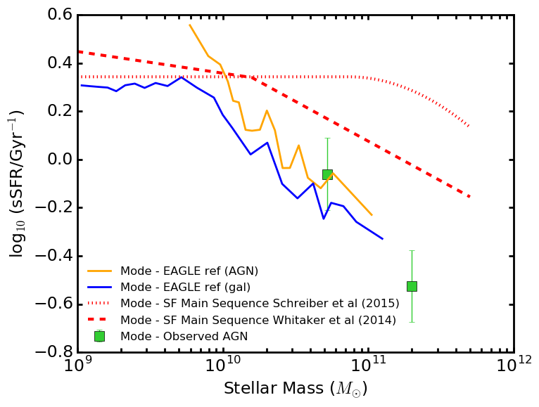
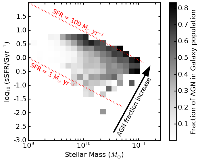
Figure 6: Top Panel: sSFR versus stellar mass for the X-ray AGN in our main sample and AGN and galaxies in the EAGLE ref model. The green filled squares indicate the mode of the sSFR distributions for the observed X-ray AGN with error bars representing the $68\%$ confidence interval (see Table 3) and are compared to the modes of the AGN (orange curve) and galaxies (blue curve) from the EAGLE ref model, coeval ($z\approx$ 2.2) main sequence galaxies from Schreiber et al. (2015) (red dotted line) and Whitaker et al. (2014) (red dashed line). The mode of the sSFR for AGN is higher than the overall galaxy population but lower than galaxies on the star-forming main sequence. Bottom Panel: The grey shaded regions indicate the fraction of galaxies in a given sSFR–stellar mass bin that host AGN activity (with $L_{\rm X}>10^{43}\mathrel{\rm erg\;s^{-1}}$) in the EAGLE ref model; the AGN fraction values are indicated by the greyscale bar to the right of the figure. The dotted red lines indicate constant values of SFR. The fraction of galaxies hosting AGN activity in the EAGLE ref model is a function of the SFR (illustrated by the black arrow).

4.2 Identifying the signature of AGN feedback on the star forming properties of galaxies

Our analyses of the EAGLE simulation in §4.1 suggested that AGN have elevated sSFRs when compared to the overall galaxy population. Furthermore, both the data and the model do not reveal a negative trend between sSFR and AGN luminosity (see Figure 4). These results may appear counter intuitive for a model in which AGN feedback quenches star formation in galaxies. Therefore, what is the signature of AGN feedback on the star-forming properties of galaxies? This question can be explored from a comparison of the sSFR properties of galaxies and AGN for two different EAGLE models: the EAGLE ref model with AGN feedback and the EAGLE noAGN model, which is identical to that of the EAGLE ref model except that black holes are not seeded in this model and consequently there is no AGN activity and no AGN feedback (see §2.3).

We calculated the running mode and width of the sSFR distributions for the galaxies in both the EAGLE ref model and the EAGLE noAGN model in stellar-mass bins of 50 objects, following §2.2. In Figure 7 we compare the mode and width of the sSFR distributions of the galaxies between these two models. There are several clear differences between the sSFR properties of the galaxies with $>10^{10}\mathrel{\rm M_{\odot}}$ in the EAGLE ref and the EAGLE noAGN models: 1) the sSFR distribution is a factor $\approx$ 2 broader in the EAGLE ref model, 2) the mode of the sSFR is $\approx$ 0.2 dex lower in the EAGLE ref model, and 3) the slope of the mode of sSFR distribution as a function of mass is steeper in the EAGLE ref model; $-0.52\pm 0.02$ and $-0.35\pm 0.02$ for the EAGLE ref and EAGLE noAGN model, respectively, when we fitted a linear model to the data in logarithmic space. Of these three potential signatures of AGN feedback, we consider the broadening of the sSFR distribution to be the most reliable quantity for comparison with observations since it is less sensitive to calibration differences in stellar mass and SFR calculations between the observations and simulations. Furthermore, the width of the sSFR distributions is more sensitive to the effect of AGN feedback, since it is sensitive to a decrease in the sSFR for even a small fraction of the population.

In Figure 7 we compare the sSFR properties of the AGN in the EAGLE ref model to the galaxies in the same model. These signatures of AGN feedback are seen in both the AGN and galaxy population, implying that the impact of AGN feedback is slow and occurs on a timescale that is longer than the episodes of AGN activity (see Harrison, 2017; McAlpine et al., 2017). This slow impact of AGN feedback on the star forming properties helps to explain why AGN luminosity ($L_{\rm X}$) is not observed in the data for the EAGLE reference model to be a strong driver of the sSFR properties (see Figure 4); i.e., although the luminosity of the AGN may dictate the overall impact of the feedback on star formation, the observational signature of that impact on the star formation across the galaxy is not instantaneous. However, we note that since the measurements of star formation in our study are for the entire galaxy, these results do not rule out AGN having significant impact on a short timescale on the star formation in localised regions within the galaxy. Also the fact that the signature of AGN feedback is in both the AGN and the overall galaxy population implies that we do not have to solely study the AGN in order to understand the AGN feedback, i.e. constraining the sSFR distribution of overall galaxy population can help determine the effect of AGN feedback on star formation.

In Figure 7 we show how the measured sSFR properties of the AGN in our main sample compare to systems in the EAGLE ref and noAGN models. From this comparison it is clear that the broad width of the sSFR distribution for our main sample is in better agreement with the EAGLE ref model than the EAGLE noAGN model, providing indirect observational support for the AGN feedback in EAGLE. The broad width of the sSFR distribution indicates a wide range in sSFRs. This is seen in Figure 8, where we compare the sSFR versus stellar mass for the galaxies in the EAGLE ref and the EAGLE noAGN models. The clearest differences between the two models across the sSFR–stellar mass plane are the broader range of sSFRs for the galaxies in the EAGLE ref model and the presence of a population of galaxies with low sSFRs (less than $\log_{10}$(sSFR/Gyr^-1)=$-0.5$ Gyr^-1) not seen in the EAGLE noAGN model.

Since the two EAGLE models are identical except for the presence/absence of AGN feedback, perhaps unsurprisingly, we conclude that AGN are primarily responsible for creating the low sSFR (“quenched”) part of the galaxy population in the EAGLE ref model (Trayford et al., 2016). The halo mass quenching which is present in both models is partially responsible for a small decrease of sSFR with stellar mass, but does not reproduce the observed width and mode of the sSFR distributions (see Figure 7). Importantly, the EAGLE ref model was not calibrated to reproduce the properties of (s)SFR distributions at any redshift but successfully reproduces the parameters we measured from our observations. We have shown that we would not expect to see a strong signature of AGN feedback in trends of sSFRs as a function of AGN luminosity, but instead in the reduced mode and increased width of the sSFR distributions for the most massive galaxies.

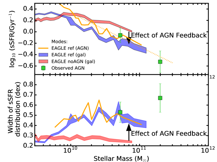
Figure 7: Mode of the sSFR (top panel) and width of the sSFR (bottom panel) versus stellar mass for the X-ray AGN in our main sample and two different EAGLE models. The solid green squares indicate the measurements from the X-ray AGN in our main sample; the error bars indicate the $68\%$ confidence interval (see Table 3). The blue and red shaded regions indicate the modes and widths of the sSFR for galaxies in the EAGLE ref model and the EAGLE model without AGN, respectively. The orange solid line indicates the modes and widths of the sSFR for AGN in the EAGLE ref model and the orange dashed line in the top panel indicates the linear extrapolation to higher stellar masses.

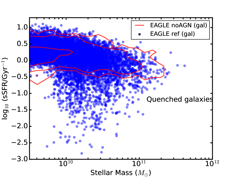
Figure 8: Individual galaxies from the EAGLE ref (blue points) and 1, 2 and 3 $\sigma$ contours (red lines) of the galaxies in the EAGLE noAGN model on the sSFR–stellar mass plane. In the EAGLE noAGN model, there are no galaxies with $\log_{10}$(sSFR/Gyr^-1)<$-0.5$ Gyr^-1. The sSFR distributions in the EAGLE ref model is a factor $\approx$ 2 broader than in the EAGLE noAGN model.

5 Conclusions

We observed 114 X-ray selected AGN with ALMA at $870\mu$m across a broad range in luminosity ($L_{\rm X}=5\times 10^{39}-10^{45}\mathrel{\rm erg\;s^{-1}}$) and redshift ($z=0.1-4.6$). Utilising the ALMA data in combination with archival Herschel and Spitzer data, we fitted the broad-band SEDs to obtain SFR and stellar-mass measurements uncontaminated by AGN emission. In the current paper we focused our analyses on a main sample of 81 X-ray selected AGN (irrespective of ALMA coverage) at $z=1.5-3.2$ with $L_{\rm X}=10^{43}-10^{45}\mathrel{\rm erg\;s^{-1}}$ and stellar mass of $>2\times 10^{10}\mathrel{\rm M_{\odot}}$. We used the SFR and stellar-mass measurements to parameterise the sSFR distributions as a function of X-ray luminosity and stellar mass, taking into account of both detections and upper limits using Bayesian techniques. To assist in the interpretation of our results, we made comparisons to the predictions from two different models from the EAGLE hydrodynamical cosmological simulation: the reference model (EAGLE ref model), which includes AGN feedback, and a model without black holes which, consequently, does not include AGN feedback (EAGLE noAGN). On the basis of our analyses we obtained the following results:

1. We found no strong ($>3$ $\sigma$) observational evidence for differences in the mode or width of the sSFR distribution for the AGN in our main sample as a function of $L_{\rm X}$. The lack of a dependence on the sSFR properties with $L_{\rm X}$ rules out a simple AGN-feedback model where high-luminosity AGN instantaneously shut down star formation. However, we do find good agreement between the properties of the sSFR distributions of our main sample and the EAGLE ref model as a function of both $L_{\rm X}$ and stellar mass, although only when the samples are matched in mass. This result indicates the importance of taking account of stellar mass in sSFR comparisons. See §3.1 and §3.2.

2. From a comparison of the properties of the sSFR distributions of the galaxies in the EAGLE ref model to the galaxies in the EAGLE noAGN model we identified a clear signature of AGN feedback on the star forming properties of galaxies. We found that the sSFR distribution is significantly broader (by a factor of $\approx$ 2) for the galaxies in the EAGLE ref model above $2\times 10^{10}\mathrel{\rm M_{\odot}}$ due to the presence of a significant population of “quenched” galaxies with low sSFRs. The broad width of the sSFR distribution of the observed population is in better agreement with the EAGLE ref model than the EAGLE nonAGN model, providing indirect evidence for AGN feedback. See §4.1 and §4.2.

Overall, from the combination of the observations with the model predictions, we conclude that (1) even with AGN feedback, there is no strong relationship between the sSFR distribution parameters and instantaneous AGN luminosity, indicating that the impact of AGN feedback on star formation is slow and (2) a signature of AGN feedback is a broad distribution of sSFRs for all galaxies regardless of whether they host a AGN or not, with M_∗> $10^{10}$M_⊙, which implies the presence of a population of “quenched” galaxies with low sSFRs. With future larger samples of AGN and galaxies with sensitive sSFR measurements (e.g., from deeper ALMA observations and other SFR tracers) we aim to measure the sSFR distribution parameters of all galaxies to greater accuracy to further constrain the role of AGN in models of galaxy formation.

Appendix A ALMA observations and catalogues

In this appendix we describe the band 7 (870 $\mu$m) ALMA observations and the construction of the ALMA catalogues for the X-ray AGN observed from our cycle 1 (project 2012.1.00869.S; PI: J. Mullaney) and cycle 2 (project 2013.1.00884.S; PI: D. Alexander) programmes. A subset of the ALMA-observed X-ray AGN are used in our main analyses, as described in §2, and SFR constraints for all of the ALMA-observed X-ray AGN at $z>1$ are presented in Stanley et al. (in prep); we note here that the SFRs in Stanley et al. (in prep) can differ by up-to $0.1$ dex from those presented here due to a slightly different method adopted to select the best-fitting SED solution (see §2.1.2).

Here we provide an overview of the ALMA target selection (see §A.1), the details of the ALMA observations (see §A.2), the reduction of the ALMA data (see §A.3), the detection of ALMA sources and the matching of ALMA-detected sources to X-ray AGN, including ALMA upper limits for the X-ray AGN that are undetected by ALMA (see §A.4).

A.1 ALMA target selection

All of the ALMA-selected targets from our Cycle 1 and Cycle 2 programmes are X-ray AGN that are detected in either the 4 Ms Chandra Deep Field South (CDF-S; Xue et al. 2011) or the Chandra Cosmic Evolution Survey (COSMOS) surveys (Civano et al. 2009; Elvis et al. 2009). The overall target selection criteria were X-ray AGN at $z>1.5$ with $L_{\rm X}>10^{42}\mathrel{\rm erg\;s^{-1}}$, for the reasons outlined in §2.1; however, we also note that the lower limit on the redshift selection was also required to make the most efficient use of ALMA for SFR constraints since the sensitivity of Herschel for measuring SFRs is comparable to, or better than, ALMA at $870\mu$m for sources at $z<1.5$ (see Casey et al. 2014 for a general review).

For the X-ray AGN in CDF-S we selected sources across the whole of the Chandra-observed region while for COSMOS we selected sources from the central $12.5^{\prime}$-radius region for X-ray AGN with $L_{\rm X}=(1-3)\times 10^{44}\mathrel{\rm erg\;s^{-1}}$ and from the central $25^{\prime}$-radius region for X-ray AGN with $L_{\rm X}=(0.3-1)\times 10^{45}\mathrel{\rm erg\;s^{-1}}$; the larger region for the AGN with $L_{\rm X}=(0.3-1)\times 10^{45}\mathrel{\rm erg\;s^{-1}}$ was required to allow for a comparable number of AGN as that in the $L_{\rm X}=(1-3)\times 10^{44}\mathrel{\rm erg\;s^{-1}}$ bin. IR-based star forming luminosity constraints were obtained for all of the X-ray AGN in CDF-S and COSMOS that met these criteria from fitting the Spitzer–Herschel IR SEDs with AGN and star forming templates, following Stanley et al. (2015). These star formation luminosity constraints were used to select X-ray AGN to observe with ALMA, with the majority of the selected targets having star formation luminosity upper limits.

Overall we selected 30 X-ray AGN in CDF-S to observe in Cycle 1 and 86 X-ray AGN in CDF-S and COSMOS to observe in Cycle 2 for 116 targets overall. The X-ray AGN selected for the Cycle 1 observations had redshifts of $z=$ 1.5–4.0 and the majority had X-ray luminosities of $L_{\rm X}\approx 10^{42}-10^{44}\mathrel{\rm erg\;s^{-1}}$, with a minority at $L_{\rm X}>10^{44}\mathrel{\rm erg\;s^{-1}}$. The X-ray AGN selected for the Cycle 2 observations were typically more luminous than in Cycle 1 ($L_{\rm X}\approx 10^{43}-10^{45}\mathrel{\rm erg\;s^{-1}}$) and covered the narrower redshift range of $z=$ 1.5–3.2.

A.2 ALMA observations

From the 116 X-ray AGN that we proposed for ALMA observations in cycle 1 and cycle 2 (see §A.1), 107 were observed; the 9 X-ray AGN not observed were Cycle 2 targets in the CDF-S at $z=$ 1.5–2.0. The 107 X-ray AGN were observed by ALMA in band 7 using a fixed continuum correlated setup with $7.5$ GHz of bandwidth centered at $344$ GHz (870 $\mu$m) and four 128-channel dual-polarisation basebands. The ALMA pointings were centered on the optical counterpart positions of the X-ray sources. The Cycle 1 data for project 2012.1.00869.S were taken on 2013 November 2 and 2013 November 16–17 using thirty-two 12 m antennas and nine 7 m antennas in the compact array (see also Mullaney et al. 2015 for details). The Cycle 2 data for project 2013.1.00884.S were taken on 2014 September 2, 2014 December 31, and 2015 January 1–2 using thirty-four 12 m antennas and nine 7 m antennas in the compact array.

The requested spatial resolution for both programmes was $\approx 1^{\prime\prime}$ to ensure that the measured 870 $\mu$m continuum emission was from the entire galaxy (physical scales of $\approx$ 7.0–8.5 kpc over the redshift range of $z=$ 1.5–4.0 for our assumed cosmology) to remove the need to apply aperture-correction factors to match the lower-resolution Spitzer and Herschel infrared data. However, the ALMA observations were taken with a variety of baselines across both programmes (91–393 m), which leads to some variation in the spatial resolution ($0^{\prime\prime}.18$-$0^{\prime\prime}.85$); see Tables 5 & 6 for the measured median baseline for each target.

The requested sensitivity for each target was broadly based on that required to detect star-formation emission from systems that lie on or below the star-forming galaxy main sequence (e.g. Schreiber et al., 2015; Whitaker et al., 2014). For the Cycle 1 programme the sensitivity limits were determined taking account of both the stellar mass and redshift of each X-ray AGN (see Mullaney et al., 2015, for more details) for more while for the cycle 2 programme only the redshift was taken into account. On the basis of these parameters, the proposed root mean squared (RMS) sensitivities varied over 0.075–0.24 mJy. However, the final sensitivities often deviated from the proposed sensitivities due to either non-optimal conditions or baseline configurations (i.e., a more extended array configuration than proposed). The final RMS sensitivities were re-measured from the tapered images (see §A.3); the final RMS sensitivities measured for each target are given in Tables 5 & 6.

A.3 ALMA data reduction

Our data reduction and source detection approach follows that described in Simpson et al. (2015). Here we provide a brief description of the procedures.

The data were imaged using the Common Astronomy Software Application (CASA version 4.4.0). The uv-visibilities were Fourier transformed to create “dirty” images. These dirty images were consequently “cleaned” using a similar technique to that described by Hodge et al. (2013); cleaning is a common technique applied to interferometric data to reduce the strength of the side lobes from bright sources to allow for the detection of faint sources. We used an iterative approach to cleaning the images. We estimated the RMS in the dirty maps and we cleaned the maps to 3 $\sigma$ (i.e., until peaks down to 3 $\sigma$ become identifiable). We then estimated the RMS in the cleaned maps and identified any objects at $\geqslant$ 5 $\sigma$. If a source was detected at $\geqslant$ 5 $\sigma$ then the cleaning process was repeated on the cleaned map in a tight region around the detected source. If a source was not detected at $\geqslant$ 5 $\sigma$ then the cleaned map was adopted as the final map.

To ensure that the 870 $\mu$m emission is measured over a common physical size scale for all of the targets, we “tapered” all of the images to give a synthesized beam of $0^{\prime\prime}.8$; this size scale was chosen to provide 870 $\mu$m constraints from the entire galaxy to allow for consistent comparisons with the lower-resolution Spitzer–Herschel data. We applied a Gaussian taper which lowers the weighting given to the long baselines to increase the size of the synthesised beam. However, this procedure also increases the noise of the maps by up-to a factor of $\approx$ 6 for the highest-resolution data. All final maps and all measured 870 $\mu$m properties have the same spatial resolution of $0^{\prime\prime}.8$.

A.4 ALMA source detection and source properties

The final maps described in §A.3 were used to detect ALMA sources. To construct a catalogue of ALMA-detected sources we require a clear detection threshold to reliably distinguish between spurious sources and real detections. To provide an assessment of the rate of spurious sources as a function of detection threshold, we created inverted maps by multiplying the final maps by $-1$. These inverted maps have the same noise properties as the original maps but they do not contain any positive peaks due to real sources (all real sources will have negative peaks).

To estimate the number of spurious sources in our final maps we compared the ratio of sources “detected” in both the final maps and inverse maps as a function of the detection threshold. To achieve this we extracted all positive peaks of at least 2.5 $\sigma$ from the cleaned maps corrected for the primary beam, and the inverted maps using Source Extractor (Bertin & Arnouts, 1996). Since we are only interested here in the ALMA properties of X-ray sources, rather than performing a blind search for ALMA sources, our total source-detection region size is substantially smaller than the combined area for all of the ALMA images. Consequently, we can detect sources down to lower significance levels than would be possible from a blind source-detection approach. We therefore split the number of detected peaks in the final and inverse ALMA maps into three different $\sigma$ bins: $2.5-3$ (low-significance peaks), $3-4$ (medium-significance peaks) and $>4$ (high-significance peaks). Adopting a search radius of $0.5^{\prime\prime}$, we calculate a total of $2.41$, $0.89$ and $0.052$ spurious objects for the $\sigma$ bins of 2.5–3, 3–4, and $>4.0$, respectively. Since the spurious fraction for the high-significance bin was so small, we increased the search radius of this bin to $1^{\prime\prime}$, which still gives a low $0.20$ spurious sources.

In matching ALMA sources to X-ray sources we therefore adopted a $0^{\prime\prime}.5$ radius for low and medium significance ALMA sources and a $1^{\prime\prime}$ radius for high-significance ALMA sources. With this source-matching approach we identified ALMA counterparts with a $\sigma\geqslant 2.5$ ALMA detection for 20 X-ray sources in CDF-S and 20 X-ray sources in COSMOS. Example HST and ALMA images of the X-ray sources are shown in Fig. 9 to demonstrate the quality of the optical and ALMA data. The ALMA detection rate is comparable between X-ray sources with photometric and spectroscopic redshifts, suggesting that inaccurate redshifts are not a major reason for the non-detections. Although our matching radii were $0.5^{\prime\prime}$ and $1^{\prime\prime}$, $\sim 80\%$ of the ALMA counterparts lie within $0.3^{\prime\prime}$ or less from the optical position of the X-ray sources, including all of the 7 low-significance ALMA sources giving us confidence that the majority are real sources.

The positions, redshifts and ALMA $870\mu$m fluxes are summarised in Tables 5 & 6. In addition to the 107 primary targets, there were a further 7 X-ray sources that serendipitously lay within the field-of-view of the primary beam of some of our ALMA maps. As a result we have ALMA coverage for 60 and 54 X-ray sources in the CDF-S and COSMOS fields respectively, covering a $L_{\rm X}$ range of $5\times 10^{39}-10^{45}\mathrel{\rm erg\;s^{-1}}$ and a redshift range of $z=$ 0.1–4.6; see Fig.  1 for the $z$–$L_{\rm X}$ coverage. For the X-ray sources without an ALMA counterpart, we calculated $3\sigma$ upper limits directly from the map. In Fig.  10 we show the ALMA 870 $\mu$m flux density versus redshift for the 114 X-ray sources with ALMA coverage.

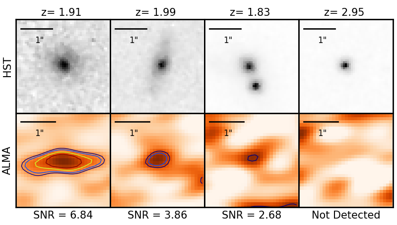
Figure 9: Example HST (H-band: $1.6\mu$m; top) and ALMA ($870\mu$m; bottom) images of X-ray AGN to indicate the range in $\sigma$ (SNR) from our ALMA data. All images are $3^{\prime\prime}\times 3^{\prime\prime}$ in size; the solid bar indicates $1^{\prime\prime}$, which corresponds to $\approx$ 8 kpc over the redshift range for our main sample. The plotted contours indicate the 2.5, 3.0, 4.0, and 5.0 $\sigma$ levels for the ALMA data.

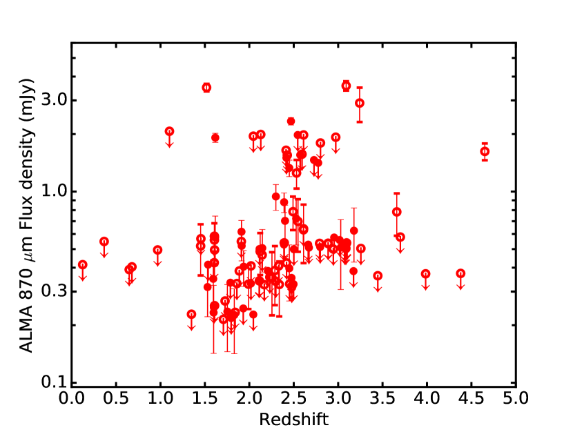
Figure 10: ALMA 870 $\mu$m flux density versus redshift for the X-ray detected that lie within our ALMA observations. The error bars represent the $1\sigma$ error on the flux density.

Table 5: X-ray selected sources observed with ALMA at $870\mu$m in CDF-S field. The columns show X-ray ID (from Hsu et al., 2014), optical positions, ALMA positions, redshift (2 and 3 decimal places indicate photometric and spectroscopic redshifts, respectively), X-ray luminosity (rest-frame 2-10 keV), primary beam corrected ALMA fluxes, median baseline of the ALMA configuration, the RMS of the map containing the X-ray AGN and the observing ID.

X-ray ID	RA Optical	Dec Optical	RA ALMA	Dec ALMA	redshift	log10	F870μm	Median baseline	RMS	Observing ID
	(J2000)	(J2000)	(J2000)	(J2000)		(L2-10keV/erg s-1)	(mJy)	(m)	(mJy)
$88$	$53.01019$	$-27.76674$	$53.01025$	$-27.76677$	$1.616$	$43.5$	$0.58\pm 0.17$	220	$0.168$	2012.1.00869.S
$93$	$53.01265$	$-27.74724$			$2.573$	$43.5$	$<1.87$	393	$0.622$	2013.1.00884.S
$123$	$53.02794$	$-27.74866$			$2.33$	$42.7$	$<0.49$	220	$0.163$	2012.1.00869.S
$129$	$53.02961$	$-27.87481$			$3.45$	$43.8$	$<0.44$	91	$0.145$	2013.1.00884.S
$137$	$53.03333$	$-27.78258$			$2.610$	$43.9$	$<0.76$	220	$0.252$	2012.1.00869.S
$155$	$53.04094$	$-27.83607$			$2.02$	< $42.5$	$<0.49$	220	$0.163$	2012.1.00869.S
$156$	$53.04098$	$-27.83766$	$53.04108$	$-27.83774$	$4.65$	$43.6$	$1.62\pm 0.16$	220	$0.163$	2012.1.00869.S
$158$	$53.04264$	$-27.86558$			$2.05$	$42.7$	$<2.34$	393	$0.780$	2013.1.00884.S
$163$	$53.04495$	$-27.77439$			$1.607$	< $42.3$	$<0.67$	220	$0.223$	2012.1.00869.S
$167$	$53.04567$	$-27.81557$			$1.46$	$43.1$	$<0.68$	220	$0.227$	2012.1.00869.S
$184$	$53.05220$	$-27.77477$			$1.605$	$42.3$	$<0.51$	220	$0.170$	2012.1.00869.S
$185$	$53.05233$	$-27.82728$	$53.05237$	$-27.82737$	$2.34$	< $42.4$	$0.33\pm 0.10$	220	$0.104$	2012.1.00869.S
$195$	$53.05584$	$-27.81555$	$53.05584$	$-27.81566$	$1.45$	$42.9$	$0.52\pm 0.16$	91	$0.155$	2013.1.00884.S
$199$	$53.05786$	$-27.83350$			$2.42$	$43.1$	$<1.80$	393	$0.601$	2013.1.00884.S
$211$	$53.06190$	$-27.85105$			$1.60$	$43.2$	$<0.30$	220	$0.099$	2012.1.00869.S
$215$	$53.06326$	$-27.69964$	$53.06326$	$-27.69971$	$2.402$	$43.1$	$0.70\pm 0.15$	91	$0.146$	2013.1.00884.S
$221$	$53.06567$	$-27.87887$			$1.89$	$42.4$	$<0.46$	220	$0.154$	2012.1.00869.S
$230$	$53.06774$	$-27.92342$	$53.06781$	$-27.92361$	$3.98$	$43.7$	$0.43\pm 0.15$	91	$0.149$	2013.1.00884.S
$249$	$53.07446$	$-27.84980$			$0.124$	< $39.8$	$<0.50$	220	$0.166$	2012.1.00869.S
$254$	$53.07600$	$-27.87816$			$2.801$	$43.1$	$<2.16$	393	$0.719$	2013.1.00884.S
$257$	$53.07640$	$-27.84866$			$1.536$	$43.7$	$<0.50$	220	$0.166$	2012.1.00869.S
$262$	$53.07846$	$-27.85986$	$53.07840$	$-27.86004$	$3.660$	$43.8$	$0.78\pm 0.20$	220	$0.195$	2012.1.00869.S
$276$	$53.08270$	$-27.86657$	$53.08275$	$-27.86657$	$1.52$	$42.1$	$3.50\pm 0.16$	220	$0.161$	2012.1.00869.S
$277$	$53.08313$	$-27.71198$			$2.21$	$43.4$	$<0.46$	91	$0.154$	2013.1.00884.S
$290$	$53.08732$	$-27.92955$			$2.55$	$43.6$	$<2.37$	393	$0.791$	2013.1.00884.S
$294$	$53.08918$	$-27.93047$			$2.611$	$43.3$	$<2.37$	393	$0.791$	2013.1.00884.S
$301$	$53.09229$	$-27.80316$	$53.09234$	$-27.80322$	$2.47$	$43.2$	$2.34\pm 0.10$	220	$0.104$	2012.1.00869.S
$305$	$53.09379$	$-27.80131$			$2.42$	$42.7$	$<0.51$	220	$0.169$	2012.1.00869.S
$308$	$53.09392$	$-27.76772$			$1.727$	$43.6$	$<0.32$	220	$0.107$	2012.1.00869.S
$310$	$53.09403$	$-27.80413$	$53.09404$	$-27.80419$	$2.39$	$43.1$	$0.88\pm 0.10$	220	$0.104$	2012.1.00869.S
$318$	$53.09636$	$-27.74506$	$53.09639$	$-27.74505$	$1.607$	< $42.2$	$0.58\pm 0.10$	220	$0.099$	2012.1.00869.S
$320$	$53.09765$	$-27.71528$	$53.09771$	$-27.71537$	$2.145$	$42.8$	$0.56\pm 0.19$	220	$0.186$	2012.1.00869.S
$326$	$53.10081$	$-27.71599$			$2.298$	$42.9$	$<0.41$	91	$0.136$	2013.1.00884.S
$344$	$53.10486$	$-27.70522$	$53.10487$	$-27.70532$	$1.617$	$43.4$	$1.92\pm 0.11$	220	$0.105$	2012.1.00869.S
$351$	$53.10702$	$-27.71823$	$53.10709$	$-27.71834$	$2.532$	$44.1$	$1.25\pm 0.21$	220	$0.214$	2012.1.00869.S
$359$	$53.10811$	$-27.75398$			$2.728$	$43.4$	$<1.76$	393	$0.585$	2013.1.00884.S
$371$	$53.11156$	$-27.76777$	$53.11157$	$-27.76782$	$3.24$	$43.5$	$2.91\pm 0.59$	393	$0.594$	2013.1.00884.S
$386$	$53.11783$	$-27.73430$	$53.11797$	$-27.73438$	$3.256$	< $42.9$	$0.55\pm 0.20$	220	$0.202$	2012.1.00869.S
$388$	$53.11858$	$-27.88480$			$2.13$	$42.7$	$<2.39$	393	$0.796$	2013.1.00884.S
$405$	$53.12283$	$-27.72280$			$1.609$	$42.7$	$<0.30$	220	$0.101$	2012.1.00869.S
$410$	$53.12409$	$-27.89120$	$53.12405$	$-27.89123$	$2.53$	$43.3$	$0.72\pm 0.20$	220	$0.197$	2012.1.00869.S
$412$	$53.12436$	$-27.85163$			$3.700$	$44.1$	$<0.69$	220	$0.231$	2012.1.00869.S
$422$	$53.12557$	$-27.88646$	$53.12560$	$-27.88651$	$2.49$	< $42.7$	$0.79\pm 0.16$	220	$0.156$	2012.1.00869.S
$423$	$53.12558$	$-27.88497$			$0.648$	< $41.4$	$<0.47$	220	$0.156$	2012.1.00869.S
$444$	$53.13403$	$-27.78096$			$2.39$	$43.4$	$<0.65$	220	$0.216$	2012.1.00869.S
$456$	$53.13799$	$-27.86825$			$3.17$	$43.1$	$<0.46$	91	$0.154$	2013.1.00884.S
$463$	$53.14102$	$-27.76673$			$1.910$	< $42.2$	$<0.66$	220	$0.219$	2012.1.00869.S
$466$	$53.14163$	$-27.81656$			$2.78$	$43.2$	$<1.70$	393	$0.566$	2013.1.00884.S
$470$	$53.14241$	$-27.76504$			$0.366$	< $40.7$	$<0.66$	220	$0.219$	2012.1.00869.S
$502$	$53.15118$	$-27.71608$			$0.968$	$41.9$	$<0.59$	220	$0.198$	2012.1.00869.S
$503$	$53.15119$	$-27.71373$			$1.609$	< $42.5$	$<0.59$	220	$0.198$	2012.1.00869.S
$509$	$53.15518$	$-27.74074$			$1.10$	$41.9$	$<2.48$	393	$0.828$	2013.1.00884.S
$522$	$53.15844$	$-27.77397$			$2.12$	$43.3$	$<0.60$	220	$0.200$	2012.1.00869.S
$528$	$53.16150$	$-27.85601$			$2.97$	$43.4$	$<2.31$	393	$0.770$	2013.1.00884.S
$534$	$53.16230$	$-27.71213$	$53.16240$	$-27.71222$	$4.379$	$43.5$	$0.44\pm 0.15$	91	$0.149$	2013.1.00884.S
$535$	$53.16271$	$-27.74426$			$0.679$	$42.4$	$<0.48$	220	$0.162$	2012.1.00869.S
$574$	$53.17868$	$-27.80263$			$2.43$	$42.6$	$<1.86$	393	$0.621$	2013.1.00884.S
$593$	$53.18583$	$-27.80997$			$2.593$	$43.4$	$<1.88$	393	$0.628$	2013.1.00884.S
$633$	$53.20487$	$-27.91795$	$53.20489$	$-27.91800$	$2.30$	$43.4$	$0.94\pm 0.15$	91	$0.146$	2013.1.00884.S
$677$	$53.24444$	$-27.90757$			$2.41$	$43.4$	$<1.97$	393	$0.658$	2013.1.00884.S

Table 6: X-ray selected sources observed with ALMA at $870\mu$m in COSMOS field. The columns show X-ray ID (from Marchesi et al., 2016), optical positions, ALMA positions, redshift (2 and 3 decimal places indicate photometric and spectroscopic redshifts, respectively), X-ray luminosity (rest-frame 2-10 keV), primary beam corrected ALMA fluxes, median baseline of the ALMA configuration, the RMS of the map containing the X-ray AGN and the observing ID.

X-ray ID	RA Optical	Dec Optical	RA ALMA	Dec ALMA	redshift	log10	F870μm	Median baseline	RMS	Observing ID
	(J2000)	(J2000)	(J2000)	(J2000)		(L2-10keV/erg s-1)	(mJy)	(m)	(mJy)
cid $434$	$149.72072$	$2.34901$	$149.72067$	$2.34904$	$1.530$	$44.6$	$0.32\pm 0.10$	91	$0.095$	2013.1.00884.S
cid $580$	$149.85469$	$2.60694$			$2.11$	$44.5$	$<0.41$	91	$0.135$	2013.1.00884.S
cid $1620$	$149.87585$	$2.69028$			$2.169$	$44.4$	$<0.39$	91	$0.130$	2013.1.00884.S
cid $558$	$149.88252$	$2.50513$			$3.10$	$44.8$	$<0.64$	91	$0.214$	2013.1.00884.S
cid $330$	$149.95583$	$2.02806$	$149.95575$	$2.02801$	$1.753$	$44.6$	$0.24\pm 0.09$	91	$0.090$	2013.1.00884.S
cid $529$	$149.98158$	$2.31501$			$3.017$	$44.6$	$<0.67$	91	$0.223$	2013.1.00884.S
cid $474$	$149.99390$	$2.30146$			$1.796$	$44.5$	$<0.27$	91	$0.091$	2013.1.00884.S
cid $451$	$150.00253$	$2.25863$	$150.00258$	$2.25864$	$2.450$	$44.6$	$0.40\pm 0.13$	91	$0.129$	2013.1.00884.S
cid $1127$	$150.01057$	$2.26939$			$2.390$	$44.1$	$<0.63$	91	$0.211$	2013.1.00884.S
cid $1205$	$150.01070$	$2.33297$	$150.01079$	$2.33300$	$2.255$	$43.9$	$0.35\pm 0.13$	91	$0.128$	2013.1.00884.S
cid $706$	$150.01105$	$2.36766$			$2.11$	$43.9$	$<0.41$	91	$0.137$	2013.1.00884.S
cid $1246$	$150.01559$	$2.44216$			$2.89$	$44.0$	$<0.64$	91	$0.214$	2013.1.00884.S
cid $532$	$150.01985$	$2.34914$			$1.796$	$44.4$	$<0.26$	91	$0.087$	2013.1.00884.S
cid $1216$	$150.02008$	$2.35365$			$2.663$	$44.1$	$<0.63$	91	$0.211$	2013.1.00884.S
cid $987$	$150.02727$	$2.43472$			$1.860$	$44.0$	$<0.40$	91	$0.132$	2013.1.00884.S
cid $659$	$150.03290$	$2.45859$			$2.045$	$44.0$	$<0.27$	91	$0.091$	2013.1.00884.S
cid $1214$	$150.03677$	$2.35852$	$150.03680$	$2.35843$	$1.59$	$44.0$	$0.35\pm 0.09$	91	$0.091$	2013.1.00884.S
cid $1143$	$150.03682$	$2.25778$			$2.454$	$44.0$	$<0.39$	91	$0.132$	2013.1.00884.S
cid $351$	$150.04262$	$2.06329$			$2.018$	$44.6$	$<0.40$	91	$0.132$	2013.1.00884.S
cid $708$	$150.05225$	$2.36927$	$150.05226$	$2.36935$	$2.548$	$44.0$	$0.70\pm 0.21$	91	$0.214$	2013.1.00884.S
cid $352$	$150.05891$	$2.01518$			$2.498$	$44.6$	$<0.39$	91	$0.131$	2013.1.00884.S
cid $1247$	$150.06346$	$2.42192$			$3.09$	$43.9$	$<0.61$	91	$0.202$	2013.1.00884.S
cid $1215$	$150.06454$	$2.32905$	$150.06451$	$2.32912$	$2.450$	$44.1$	$1.33\pm 0.13$	91	$0.132$	2013.1.00884.S
cid $459$	$150.06467$	$2.19098$			$2.89$	$44.7$	$<0.64$	91	$0.215$	2013.1.00884.S
cid $960$	$150.07462$	$2.30206$	$150.07455$	$2.30199$	$2.122$	$43.9$	$0.49\pm 0.12$	91	$0.120$	2013.1.00884.S
cid $1219$	$150.07600$	$2.26429$			$2.946$	$44.1$	$<0.60$	91	$0.200$	2013.1.00884.S
cid $72$	$150.09154$	$2.39908$			$2.475$	$44.6$	$<0.42$	91	$0.141$	2013.1.00884.S
cid $85$	$150.09653$	$2.29309$			$1.349$	$43.8$	$<0.27$	91	$0.091$	2013.1.00884.S
cid $467$	$150.10201$	$2.10549$	$150.10194$	$2.10550$	$2.288$	$44.8$	$0.39\pm 0.13$	91	$0.132$	2013.1.00884.S
cid $149$	$150.10371$	$2.66577$			$2.955$	$44.7$	$<0.69$	91	$0.230$	2013.1.00884.S
cid $1144$	$150.10477$	$2.24364$	$150.10469$	$2.24365$	$1.912$	$44.1$	$0.62\pm 0.09$	91	$0.090$	2013.1.00884.S
cid $86$	$150.11958$	$2.29591$	$150.11958$	$2.29595$	$1.831$	$44.3$	$0.23\pm 0.08$	91	$0.084$	2013.1.00884.S
cid $87$	$150.13304$	$2.30328$	$150.13309$	$2.30324$	$1.598$	$44.9$	$0.23\pm 0.09$	91	$0.090$	2013.1.00884.S
cid $965$	$150.15218$	$2.30785$	$150.15216$	$2.30779$	$3.178$	$44.2$	$0.62\pm 0.20$	91	$0.197$	2013.1.00884.S
cid $914$	$150.18001$	$2.23128$	$150.17992$	$2.23133$	$2.146$	$44.0$	$0.51\pm 0.13$	91	$0.127$	2013.1.00884.S
cid $81$	$150.18655$	$2.45533$	$150.18660$	$2.45530$	$1.991$	$44.0$	$0.33\pm 0.08$	91	$0.085$	2013.1.00884.S
cid $121$	$150.19180$	$2.54391$			$2.79$	$44.3$	$<0.64$	91	$0.214$	2013.1.00884.S
cid $917$	$150.19263$	$2.21985$	$150.19260$	$2.21983$	$3.090$	$43.9$	$3.58\pm 0.20$	91	$0.201$	2013.1.00884.S
cid $124$	$150.20532$	$2.50293$			$3.07$	$44.3$	$<0.63$	91	$0.211$	2013.1.00884.S
cid $953$	$150.21075$	$2.39147$			$3.095$	$44.1$	$<0.65$	91	$0.216$	2013.1.00884.S
cid $83$	$150.21416$	$2.47502$			$3.075$	$44.5$	$<0.61$	91	$0.202$	2013.1.00884.S
cid $1085$	$150.21634$	$1.98874$			$2.231$	$44.5$	$<0.43$	91	$0.143$	2013.1.00884.S
cid $915$	$150.21909$	$2.27867$			$1.84$	$44.0$	$<0.28$	91	$0.093$	2013.1.00884.S
cid $976$	$150.22527$	$2.35122$			$2.478$	$43.9$	$<0.38$	91	$0.128$	2013.1.00884.S
cid $954$	$150.23180$	$2.36401$	$150.23178$	$2.36400$	$1.936$	$44.2$	$0.40\pm 0.09$	91	$0.086$	2013.1.00884.S
cid $970$	$150.23550$	$2.36176$			$2.501$	$44.6$	$<0.60$	91	$0.200$	2013.1.00884.S
cid $75$	$150.24779$	$2.44215$	$150.24777$	$2.44216$	$3.029$	$44.7$	$0.51\pm 0.20$	91	$0.203$	2013.1.00884.S
cid $31$	$150.27214$	$2.23010$	$150.27217$	$2.23009$	$2.611$	$44.8$	$0.64\pm 0.22$	91	$0.216$	2013.1.00884.S
cid $90$	$150.28482$	$2.39505$			$1.932$	$44.4$	$<0.29$	91	$0.098$	2013.1.00884.S
cid $365$	$150.28563$	$2.01459$			$2.671$	$44.5$	$<0.61$	91	$0.204$	2013.1.00884.S
cid $58$	$150.32689$	$2.09415$			$2.798$	$44.5$	$<0.62$	91	$0.205$	2013.1.00884.S
cid $53$	$150.34372$	$2.14067$			$1.787$	$44.2$	$<0.40$	91	$0.133$	2013.1.00884.S
cid $581$	$150.35358$	$2.34220$			$1.708$	$44.5$	$<0.26$	91	$0.086$	2013.1.00884.S
cid $62$	$150.37364$	$2.11203$	$150.37366$	$2.11203$	$1.914$	$44.5$	$0.52\pm 0.09$	91	$0.086$	2013.1.00884.S

References

- Alexander & Hickox (2012) Alexander D. M., Hickox R. C., 2012, New Astron. Rev., 56, 93
- Azadi et al. (2015) Azadi M., et al., 2015, ApJ, 806, 187
- Azadi et al. (2017) Azadi M., et al., 2017, ApJ, 835, 27
- Balmaverde & Capetti (2015) Balmaverde B., Capetti A., 2015, A&A, 581, A76
- Beckmann et al. (2017) Beckmann R. S., et al., 2017, preprint, (arXiv:1701.07838)
- Bertin & Arnouts (1996) Bertin E., Arnouts S., 1996, A&AS, 117, 393
- Bower et al. (2017) Bower R. G., Schaye J., Frenk C. S., Theuns T., Schaller M., Crain R. A., McAlpine S., 2017, MNRAS, 465, 32
- Brandt & Alexander (2015) Brandt W. N., Alexander D. M., 2015, A&ARv, 23, 1
- Bruzual & Charlot (2003) Bruzual G., Charlot S., 2003, MNRAS, 344, 1000
- Burgarella et al. (2005) Burgarella D., Buat V., Iglesias-Páramo J., 2005, MNRAS, 360, 1413
- Cardamone et al. (2010) Cardamone C. N., et al., 2010, ApJS, 189, 270
- Casey et al. (2014) Casey C. M., Narayanan D., Cooray A., 2014, Phys. Rep., 541, 45
- Chabrier (2003) Chabrier G., 2003, PASP, 115, 763
- Charlot & Fall (2000) Charlot S., Fall S. M., 2000, ApJ, 539, 718
- Cicone et al. (2014) Cicone C., et al., 2014, A&A, 562, A21
- Ciesla et al. (2015) Ciesla L., et al., 2015, A&A, 576, A10
- Civano et al. (2009) Civano F. M., Elvis M., Brusa M., Chandra COSMOS Team 2009, 41, 422
- Civano et al. (2016) Civano F., et al., 2016, ApJ, 819, 62
- Cowley et al. (2016) Cowley M. J., et al., 2016, MNRAS, 457, 629
- Crain et al. (2015) Crain R. A., et al., 2015, MNRAS, 450, 1937
- Damen et al. (2011) Damen M., et al., 2011, ApJ, 727, 1
- Del Moro et al. (2013) Del Moro A., et al., 2013, A&A, 549, A59
- Elbaz et al. (2011) Elbaz D., et al., 2011, A&A, 533, A119
- Elvis et al. (2009) Elvis M., et al., 2009, ApJS, 184, 158
- Fabian (2012) Fabian A. C., 2012, ARA&A, 50, 455
- Fritz et al. (2006) Fritz J., Franceschini A., Hatziminaoglou E., 2006, MNRAS, 366, 767
- Furlong et al. (2015) Furlong M., et al., 2015, MNRAS, 450, 4486
- Ganguly & Brotherton (2008) Ganguly R., Brotherton M. S., 2008, ApJ, 672, 102
- Grogin et al. (2011) Grogin N. A., et al., 2011, ApJS, 197, 35
- Guo et al. (2013) Guo Y., et al., 2013, ApJS, 207, 24
- Harrison (2017) Harrison C. M., 2017, Nature Astronomy, 1, 0165
- Harrison et al. (2012) Harrison C. M., et al., 2012, ApJ, 760, L15
- Harrison et al. (2014) Harrison C. M., Alexander D. M., Mullaney J. R., Swinbank A. M., 2014, MNRAS, 441, 3306
- Harrison et al. (2016) Harrison C. M., et al., 2016, MNRAS, 456, 1195
- Hickox et al. (2009) Hickox R. C., et al., 2009, ApJ, 696, 891
- Hickox et al. (2014) Hickox R. C., Mullaney J. R., Alexander D. M., Chen C.-T. J., Civano F. M., Goulding A. D., Hainline K. N., 2014, ApJ, 782, 9
- Hodge et al. (2013) Hodge J. A., et al., 2013, ApJ, 768, 91
- Hsu et al. (2014) Hsu L.-T., et al., 2014, ApJ, 796, 60
- Kennicutt (1998) Kennicutt Jr. R. C., 1998, ARA&A, 36, 189
- King & Nixon (2015) King A., Nixon C., 2015, MNRAS, 453, L46
- Koekemoer et al. (2011) Koekemoer A. M., et al., 2011, ApJS, 197, 36
- Koss et al. (2011) Koss M., Mushotzky R., Veilleux S., Winter L. M., Baumgartner W., Tueller J., Gehrels N., Valencic L., 2011, ApJ, 739, 57
- Lacey et al. (2016) Lacey C. G., et al., 2016, MNRAS, 462, 3854
- Laigle et al. (2016) Laigle C., et al., 2016, ApJS, 224, 24
- Lanzuisi et al. (2017) Lanzuisi G., et al., 2017, A&A, 602, A123
- Le Floc’h et al. (2009) Le Floc’h E., et al., 2009, ApJ, 703, 222
- Leung et al. (2017) Leung G. C. K., et al., 2017, preprint, (arXiv:1703.10255)
- Lutz et al. (2010) Lutz D., et al., 2010, ApJ, 712, 1287
- Lutz et al. (2011) Lutz D., et al., 2011, A&A, 532, A90
- Madau & Dickinson (2014) Madau P., Dickinson M., 2014, ARA&A, 52, 415
- Magnelli et al. (2013) Magnelli B., et al., 2013, A&A, 553, A132
- Marchesi et al. (2016) Marchesi S., et al., 2016, ApJ, 817, 34
- McAlpine et al. (2016) McAlpine S., et al., 2016, Astronomy and Computing, 15, 72
- McAlpine et al. (2017) McAlpine S., Bower R. G., Harrison C. M., Crain R. A., Schaller M., Schaye J., Theuns T., 2017, MNRAS, 468, 3395
- McNamara & Nulsen (2012) McNamara B. R., Nulsen P. E. J., 2012, New Journal of Physics, 14, 055023
- Miller et al. (2008) Miller N. A., Fomalont E. B., Kellermann K. I., Mainieri V., Norman C., Padovani P., Rosati P., Tozzi P., 2008, ApJS, 179, 114
- Mor & Netzer (2012) Mor R., Netzer H., 2012, MNRAS, 420, 526
- Mullaney et al. (2011) Mullaney J. R., Alexander D. M., Goulding A. D., Hickox R. C., 2011, MNRAS, 414, 1082
- Mullaney et al. (2012) Mullaney J. R., et al., 2012, MNRAS, 419, 95
- Mullaney et al. (2013) Mullaney J. R., Alexander D. M., Fine S., Goulding A. D., Harrison C. M., Hickox R. C., 2013, MNRAS, 433, 622
- Mullaney et al. (2015) Mullaney J. R., et al., 2015, MNRAS, 453, L83
- Nandra et al. (2007) Nandra K., et al., 2007, ApJ, 660, L11
- Noeske et al. (2007) Noeske K. G., et al., 2007, ApJ, 660, L43
- Page et al. (2012) Page M. J., et al., 2012, Nature, 485, 213
- Rosario et al. (2012) Rosario D. J., et al., 2012, A&A, 545, A45
- Rosario et al. (2013) Rosario D. J., et al., 2013, ApJ, 771, 63
- Rovilos et al. (2012) Rovilos E., et al., 2012, A&A, 546, A58
- Sanders et al. (2007) Sanders D. B., et al., 2007, ApJS, 172, 86
- Santini et al. (2012) Santini P., et al., 2012, A&A, 540, A109
- Schawinski et al. (2015) Schawinski K., Koss M., Berney S., Sartori L. F., 2015, MNRAS, 451, 2517
- Schaye et al. (2015) Schaye J., et al., 2015, MNRAS, 446, 521
- Schreiber et al. (2015) Schreiber C., et al., 2015, A&A, 575, A74
- Schwarz, G (1978) Schwarz, G 1978, Annals of Statistics, 6
- Shao et al. (2010) Shao L., et al., 2010, A&A, 518, L26
- Shimizu et al. (2015) Shimizu T. T., Mushotzky R. F., Meléndez M., Koss M., Rosario D. J., 2015, MNRAS, 452, 1841
- Silva et al. (1998) Silva L., Granato G. L., Bressan A., Danese L., 1998, ApJ, 509, 103
- Silverman et al. (2009) Silverman J. D., et al., 2009, ApJ, 696, 396
- Simpson et al. (2015) Simpson J. M., et al., 2015, ApJ, 807, 128
- Speagle et al. (2014) Speagle J. S., Steinhardt C. L., Capak P. L., Silverman J. D., 2014, ApJS, 214, 15
- Springel (2005) Springel V., 2005, MNRAS, 364, 1105
- Springel et al. (2005) Springel V., Di Matteo T., Hernquist L., 2005, ApJ, 620, L79
- Stanley (2016) Stanley F., 2016, PhD thesis, Durham University
- Stanley et al. (2015) Stanley F., Harrison C. M., Alexander D. M., Swinbank A. M., Aird J. A., Del Moro A., Hickox R. C., Mullaney J. R., 2015, MNRAS, 453, 591
- Sturm et al. (2011) Sturm E., et al., 2011, ApJ, 733, L16
- Swinbank et al. (2014) Swinbank A. M., et al., 2014, MNRAS, 438, 1267
- Teplitz et al. (2011) Teplitz H. I., et al., 2011, AJ, 141, 1
- Trayford et al. (2015) Trayford J. W., et al., 2015, MNRAS, 452, 2879
- Trayford et al. (2016) Trayford J. W., Theuns T., Bower R. G., Crain R. A., Lagos C. d. P., Schaller M., Schaye J., 2016, MNRAS, 460, 3925
- Trayford et al. (2017) Trayford J. W., et al., 2017, preprint, (arXiv:1705.02331)
- Veilleux et al. (2005) Veilleux S., Cecil G., Bland-Hawthorn J., 2005, ARA&A, 43, 769
- Vito et al. (2014) Vito F., et al., 2014, MNRAS, 441, 1059
- Vogelsberger et al. (2014) Vogelsberger M., et al., 2014, MNRAS, 444, 1518
- Whitaker et al. (2014) Whitaker K. E., et al., 2014, ApJ, 795, 104
- Xue et al. (2011) Xue Y. Q., et al., 2011, ApJS, 195, 10