Many-body localization of bosons in optical lattices

Abstract

Many–body localization for a system of bosons trapped in a one dimensional lattice is discussed. Two models that may be realized for cold atoms in optical lattices are considered. The model with a random on-site potential is compared with previously introduced random interactions model. While the origin and character of the disorder in both systems is different they show interesting similar properties. In particular, many–body localization appears for a sufficiently large disorder as verified by a time evolution of initial density wave states as well as using statistical properties of energy levels for small system sizes. Starting with different initial states, we observe that the localization properties are energy–dependent which reveals an inverted many–body localization edge in both systems (that finding is also verified by statistical analysis of energy spectrum). Moreover, we consider computationally challenging regime of transition between many body localized and extended phases where we observe a characteristic algebraic decay of density correlations which may be attributed to subdiffusion (and Griffiths–like regions) in the studied systems. Ergodicity breaking in the disordered Bose–Hubbard models is compared with the slowing–down of the time evolution of the clean system at large interactions.

1 Introduction

The effects of interactions on disordered localized physical systems remained to a large extent a mystery for over fifty years after the pioneering work of Anderson [1] who introduced the concept of single–particle localization. The study of interactions in the metallic regime practically began with the work of Altshuler and Aronov [2], subsequently problems related to the presence of the disorder and interactions were addressed by several works (a highly incomplete list may include [3, 4, 5, 6]) also in cold atomic settings [7]. It was in the seminal paper [8] that many body localization (MBL) was identified as a genuine new phenomenon occurring for sufficiently strong disorders. This stimulated numerous studies of various aspects of the MBL in the last ten years (for reviews see [9, 10, 11, 12]). Presently, it is a common understanding that MBL is the most robust way of ergodicity breaking in the quantum world.

Most of the theoretical studies of MBL were performed for interacting spin models in a lattice, (e.g. Heisenberg, XXZ) as amply reviewed in e.g. [9, 10, 11, 12]. Those spin models were frequently mapped on spinless fermions. Experimentally, both fermionic [13, 14] as well as bosonic species [15, 16] were investigated where the latter seem to be particularly challenging. While for 1/2-spins (spinless fermions) an on–site Hilbert space is two dimensional (and for spinful fermions four dimensional), for bosons we have to effectively deal with much larger dimensions of local Hilbert space (constrained, strictly speaking, by the total number of particles, $N$) unless we want to consider the artificial case of hard-core bosons [17]. This makes bosonic systems unique.

In this work we consider MBL in the Bose–Hubbard model due to two distinct mechanisms – either resulting from random interactions (we extend here our previous studies [18, 19]) or from random on–site potential. Bosonic systems have the advantage of being easily controlled and prepared in an experiment. Moreover, the local Hilbert space is unconstrained in the bosonic case as mentioned above. That provides additional freedom in the choice of initial states and on one hand provides the experimentalist with supplementary ways of studying ergodicity breaking and on the other hand leads to more complex dynamics that makes numerical simulations of bosonic systems a challenging task.

Consider the standard Bose–Hubbard model in one dimension

$${H=-J\sum_{\langle i,j\rangle}\hat{a}^{{\dagger}}_{i}\hat{a}_{j}+\frac{U}{2}\sum_{i}\hat{n}_{i}(\hat{n}_{i}-1)+\mu\sum_{i}\hat{n}_{i}.}$$

There are two straightforward and experimentally feasible ways of introducing a genuine random disorder to the system. The Bose–Hubbard model with random on–site potential can be simulated by an optical speckle field (assuming that the correlation length of the speckle is smaller than the lattice spacing):

$${H=-J\sum_{\langle i,j\rangle}\hat{a}^{{\dagger}}_{i}\hat{a}_{j}+\frac{U}{2}\sum_{i}\hat{n}_{i}(\hat{n}_{i}-1)+\sum_{i}\mu_{i}\hat{n}_{i}}$$ (1)

with $\mu_{i}\in[-W/2,\,W/2]$. While this seems quite straightforward, a careful analysis [20] shows that a realistic tight-binding model for a random speckle potential imposed on top of an optical lattice leads to a more sophisticated model with all the parameters being random and drawn from speckle potential induced distributions. Nevertheless, later we will restrict ourselves to the model (1) as a plausible simplification of the experimental situation. Especially as the state of the art imaging under a quantum microscope [21] enables a creation of an arbitrary optical potential by appropriate holographic masks.

The second option is realized when the optical lattice is placed close to an atom chip which provides a spatially random magnetic field, that, in the vicinity of Feschbach resonance, leads to random interactions [22]

$${H=-J\sum_{\langle i,j\rangle}\hat{a}^{{\dagger}}_{i}\hat{a}_{j}+\sum_{i}\frac{U_{i}}{2}\hat{n}_{i}(\hat{n}_{i}-1)+\sum_{i}\mu\hat{n}_{i}}$$ (2)

$U_{i}\in[0,\,U]$. The latter system (2) was shown in the proceeding work [18] to be many–body localized at sufficiently large interaction strength amplitudes $U$. More careful analysis of the level statistics of the random interactions model and a preliminary observation of an inverted mobility edge were presented in [19].

Let us mention also that quasi-periodic potentials are used in fermionic experiments [13, 23] and analyzed theoretically - for most recent works see [24, 25]. We restrict ourselves to an analysis of models with random disorder, uniformly distributed in the respective intervals.

The two systems (1) and (2) are clearly physically different. In the absence of interactions, eigenstates of (1) are localized whereas the single–particle spectrum of (2) consists of Bloch–waves and is thus fully delocalized. However, as we shall show below, both models behave, to a large extent, quite similarly in the presence of the strong disorder. On one side this suggests, that MBL is a robust phenomenon – importantly its signatures are also similar for fermionic and pure spin systems. On the other side, the remaining differences point towards system specific phenomena that may be studied.

Let us set the energy and time scales by putting $J=1$ (also $\hbar=1$). The average properties of the system with random interactions are dependent on just a single scale, $U$. The features of the system with a random on–site potential are a result of an interplay between the disorder characterized by its strength $W$ and interactions $U$. Therefore, one cannot identify disorder strengths at which the properties of the two systems would be exactly the same.

The paper is structured as follows. First, in Section 2 we analyze ergodicity breaking in the disordered Bose–Hubbard systems by examining the relaxation properties of specifically prepared density–wave like initial states during the time evolution. Above certain disorder strengths, both systems fail to relax to a uniform density profile. Quantifying the degree of ergodicity breaking, we observe that it crucially depends on the energy of the initial state which leads us to the study of the level statistics of the systems in an energy–resolved way and allows us to postulate the existence of the localization edge in the system in Section 3. We provide qualitative arguments supporting the existence of the localization edge in the perturbative language in Section 4. We consider in a detailed way (Section 5) the level spacings of the random on–site potential model showing that they are consistent with our imbalance studies. Finally, in Section 6, many–body localization in the disordered system is contrasted with the slow down of thermalization in the clean system [26].

2 The imbalance decay

The Eigenstate Thermalization Hypothesis (ETH) [27, 28, 29], states that excited eigenstates of an ergodic system have thermal expectation values of physical observables. In effect, a time average of a local observable equilibrates to the microcanonical average and remains near that value for most of the time. In order to investigate ergodicity breaking in the considered systems, we adapt a strategy analogous to the experiment [13] and study the time evolution of highly excited out–of–equilibrium states. For fermions the standard interaction mechanism is related to collisions of opposite spin fermions at a given site. Similarly, for the interaction between bosons to take place one needs at least two bosons at a single site. Therefore, as the initial state we typically consider the density wave-like Fock state $|DW_{21}\rangle=|2121...\rangle$ (working at 3/2 filling). Quantitative results are obtained via the measurement of the imbalance

$${I(t)=\frac{D(t)}{D(0)}\quad\mathrm{with}\quad D(t)=N_{e}(t)-N_{o}(t),}$$ (3)

where $N_{e,o}$ are populations of even and odd sites of the 1D lattice respectively. A non–zero stationary value of imbalance at large times shows that the system breaks ergodicity, which, in the context of an interacting many–body quantum system implies that it is many–body localized.

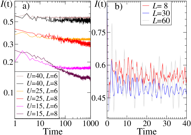
Figure 1: Decay of $I(t)$ for $|DW_{21}\rangle$ state as a function of time. Results for the random interactions system (2) with $N=9$ and $N=12$ bosons on $L=6$ and $L=8$ sites respectively on the left. The log-log scale facilitates observation of the emergence and breakdown (at times $t$ larger than the Heisenberg time $T_{H}$) of the algebraic decay of the imbalance $I(t)$. Right – comparison between $L=8,30,60$ lattice sizes for the random potential system (1) at $U=1$.

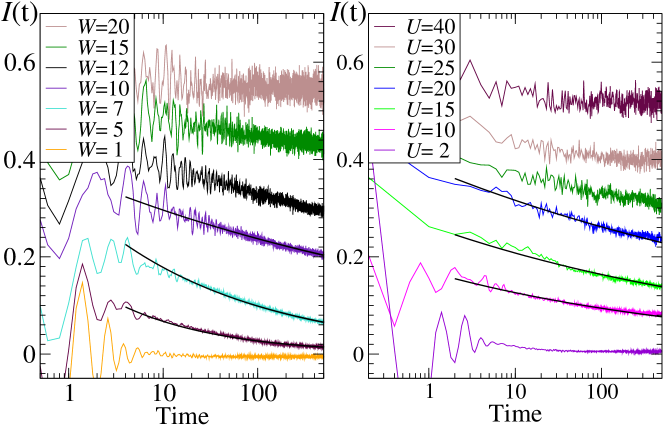
Figure 2: Decay of $I(t)$ for $|DW_{21}\rangle$ state as a function of time for $N=12$ bosons on $L=8$ lattice sites – random on–site potential with $U=1$ on the left and random interactions on the right. The horizontal axis is in logarithmic scale which facilitates observation of slow decay of $I(t)$ in the intermediate regime between many–body localized and the ergodic phases. Data corresponding to the critical region are fitted by power–law decay.

Two complementary numerical tools may be used to study the time evolution of the system starting from a high energy nonstationary state (as e.g. $|DW_{21}\rangle$). For small system sizes one may use the exact diagonalization approach and calculate the evolution operator after finding eigenvalues and eigenvectors of the problem. Such an approach has been used for (less demanding computationally) spin systems [30, 31] and allows one to reach long time dynamics. A bit larger systems may be quite efficiently emulated using time propagation in Krylov subspaces [32] - the method often referred to as the Lanczos approach, however, the calculations become more computationally demanding with the increasing evolution time.

For finite size systems the Heisenberg time $T_{H}$ (being essentially the inverse of the mean level spacings) sets a time scale at which the time evolution freezes. This is illustrated in Fig. 1a where the decay of the imbalance $I(t)$ for the system of $N=9$ bosons on $L=6$ lattice sites with interaction strength amplitude $U=15$ effectively stops at $T_{H}\approx 70$ (the dimension of the Hilbert space is equal to $2002$). However, already for $L=8$ the Hilbert space dimension is $50388$ and the Heisenberg time is $T_{H}\approx 500$ which allows for a clear observation of the decay of the imbalance $I(t)$. Fig. 1b demonstrates the effect of the system size and role of the number of disorder realizations $n$. Data for $L=8$ and $L=30$ show that the imbalance $I(t)$, after an initial transient, oscillates around a certain stationary value which decreases slightly for larger system sizes (also visible in Fig. 1a for $U=40$). Moreover, the amplitude of the oscillations decreases like $1/\sqrt{n}$ with number of disorder realizations being $n=50$ for $L=8,30$ and $n=10$ for $L=60$.

The obtained time evolution of the imbalance averaged over $50$ disorder realizations for different disorder strengths is presented in Fig. 2 for L=12 bosons on N=8 sites with open boundary conditions. At small disorder strengths both systems obey ETH and the density pattern of the $|DW_{21}\rangle$ state relaxes to uniform density – this is the case for $W=1$ (left panel) and $U=2$ (right panel). For large disorder, on the other hand, after a rapid initial decay, the imbalance saturates at a disorder strength dependent non-zero value showing quite significant fluctuations in time (as well as between different realizations of the disorder - not shown). The non-zero value of the long-time imbalance indicates that the system remembers its initial state which is the commonly used indicator of the MBL phase. In the broad transition regime between the two phases the decay of $I(t)$ is well fitted by an algebraic decay $I(t)\propto t^{-\frac{1}{z}}$ with the exponent $\frac{1}{z}$ decreasing with the increasing disorder strength (the decay slows down). This is a similar behavior to that observed in fermionic and spin systems [33, 34, 35, 31] as well as experimentally for spinful fermions [23]. In this region, which we call a quantum critical region [36, 37, 38], transport is claimed to be subdiffusive and dominated by Griffiths–type dynamics [39, 40]. According to the Griffiths phase model of the MBL transition [36, 37, 41] $z$ is the dynamical exponent associated with the transport which reaches $\frac{1}{z}=0.5$ in the diffusive limit [23]. As the border of MBL phase is approached, the exponent $\frac{1}{z}$ vanishes. Let us stress that both bosonic systems, despite a richer local Hilbert space than for spin/fermion models, share very similar subdiffusive characteristics with, e.g. $\frac{1}{z}\approx 0.4$ for $W=5$ while $\frac{1}{z}\approx 0.09$ for $W=10$. Let us also note that the size of this quantum critical region is system size dependent as discussed in detail e.g. in [38].

The analysis with Lanczos time propagation due to the exponentially increasing Hilbert space size is necessarily restricted to moderate system sizes. On the other hand, tDMRG [42, 43, 44, 45] allows one to efficiently study systems with a moderate growth of the entanglement in time - a situation expected for localized and close to localized systems. In particular, it is well known that the entanglement entropy in the MBL phase for initially uncorrelated parts grows logarithmically in time [46, 9], which allows us to study very large systems [18]. Here, we consider the time–evolution close to the MBL phase for 90 bosons distributed between $L=60$ sites (a typical size for cold-atoms experiments) to infer properties of the localized system as well as to get a glimpse of dynamics near the MBL transition – Fig. 3. In all tDMRG calculations we use open boundary conditions as realized in quasi-one-dimensional experimental situations.

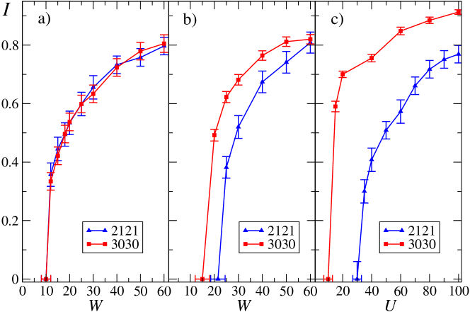
Figure 3: Stationary value $I$ of imbalance as a function of the disorder strength for for two initial Fock states: $|DW_{21}\rangle$ and $|DW_{30}\rangle$ for 90 bosons on 60 lattice sites. Panel a) corresponds to a random chemical potential in a model of weakly interacting bosons $U=1$. Within statistical errors both states have similar threshold value of non-zero imbalance around $W=10$ and show essentially the same behavior. Panel b) corresponds to the same model with stronger interactions $U=5$. Now the state localize at different value of the disorder amplitude. For random interactions an even stronger dependence on the initial state is observed – panel c).

The stationary value of imbalance can be thought of – in analogy to an order parameter in conventional phase transitions – as a quantity which determines the degree of ergodicity breaking in the system. It is straightforward to obtain the stationary imbalance deep in the many–body localized phase – performing time evolution with tDMRG we observe that $I(t)$ after initial transient (up to $t\approx 10$) saturates at a disorder strength dependent level exhibiting residual fluctuations in time. Therefore, we average $I(t)$ over a time interval in the vicinity of $t=30$. The stationary value of the obtained imbalance is further averaged over (typically ten) disorder realizations.

As the disorder strength decreases, the subdiffusive regime with the algebraic decay of the imbalance is approached. This is accompanied with a much faster build up of the entanglement which, in turn, reduces the obtainable final propagation time but, on the other hand, confirms the vicinity of the transition. The representative stationary values of the imbalance are presented in Fig. 3 for $|DW_{21}\rangle$ as well as a different density like state $|DW_{30}\rangle=|3030...\rangle$. Observe a striking difference between the left and the middle panels of Fig. 3 that correspond to different interaction strengths $U=1$ and $U=5$, respectively. The fate of both initial states for $U=1$ is very similar, they begin to show non–zero stationary imbalance around the amplitude of random chemical potential $W=10$. $I(t)$ dependence on $W$ for both states is practically identical (compare error bars). The situation drastically changes for $U=5$ where $|DW_{30}\rangle$ state localizes for much lower values of $W$. This may be attributed (and will be further confirmed in the next Section) to the significant difference in initial energies of both states.

Imbalances obtained for the model with random interactions are shown in Fig. 3c. As for the $U=5$ case discussed above, the $|DW_{30}\rangle$ initial state leads to a larger value of the stationary imbalance than the $|DW_{21}\rangle$ for a given disorder strength. Also, the disorder strength needed to obtain the non–zero stationary value of imbalance is smaller for the $|DW_{30}\rangle$ state than for the $|DW_{21}\rangle$ state. The $|DW_{30}\rangle$ state has higher energy than $|DW_{21}\rangle$ state as the interaction term grows quadratically with the number of bosons occupying a lattice site. Thus, also for this model the degree of ergodicity breaking depends on the energy of the initial state. The energy dependence of the MBL phenomenon in both systems leads us to the next section where we examine the properties of the full energy spectra by exact diagonalization.

3 Localization edge

The theory of metal-insulator transition [47] implies that the mobility (localization) edge separates in energy localized and extended states, at least in the thermodynamic limit. For interacting systems in the presence of disorder, numerical evidence for the presence of many–body mobility edges were presented for the random field Heisenberg spin chain [30] and for the fermionic Hubbard system [48, 49].

To address the properties of the system as a function of energy in a systematic way we follow [30] and analyze the statistics of energy eigenvalues using a convenient measure - the gap ratio [50]. Let $\delta_{n}$ be a difference between adjacent energies in the ordered spectrum, $\delta_{n}=E_{n+1}-E_{n}.$ The (dimensionless) gap ratio is defined as:

$$r_{n}=\min\{\delta_{n},\delta_{n-1}\}/\max\{\delta_{n},\delta_{n-1}\}.$$ (4)

It has been shown [50] that the mean of the $r_{n}$ distribution, $\overline{r}$, describes the character of the eigenstates well. For delocalized disordered states one intuitively expects a situation resembling random matrices. For time reversal invariant systems, the Gaussian Orthogonal Ensemble (GOE) of random matrices is appropriate. In this case, the mean gap ratio, $\overline{r}$, can be calculated approximately [51] yielding $\overline{r}_{GOE}=0.53$. In the opposite case, deep in the MBL phase, it is conjectured that the system is integrable and can be characterized by a complete set of local integrals of motion (LIOMs) [52, 9, 53]. As such, the spectrum should share properties with the Poisson ensemble, with the mean ratio equal to $\overline{r}_{Poisson}=2\log 2-1\approx 0.39$ [51]. In the transition regime between these two phases one expects that the mean ratio has intermediate values smoothly interpolating between the limiting cases. Such a situation has been indeed observed in a number of studies [50, 54, 30, 31, 18].

We shall characterize the studied systems with the help of $\overline{r}$ in an energy resolved way. To that end, for each value of the disorder strength (being $W$ or $U$ depending on the studied system), we collect more than $10^{6}$ eigenvalues for about 200 disorder realizations. We drop the lowest 1% of energy levels, let us denote the lower bound of the set of eigenvalues as $E_{bot}$. Similarly, we disregard the highest 1% of eigenvalues and define as $E_{top}$ the upper bound of the considered set. We rescale the members of the set as $\epsilon=(E-E_{bot})/(E_{top}-E_{bot})$ mapping the energies onto $[0,1]$. Finally, we group $\epsilon$ values in 20 equal intervals and find $\overline{r}$ in each of them separately.

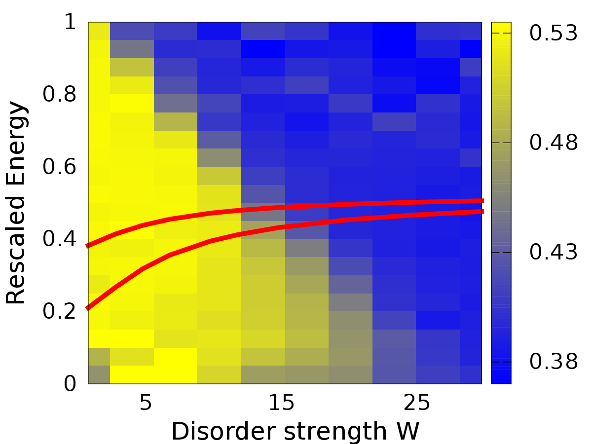
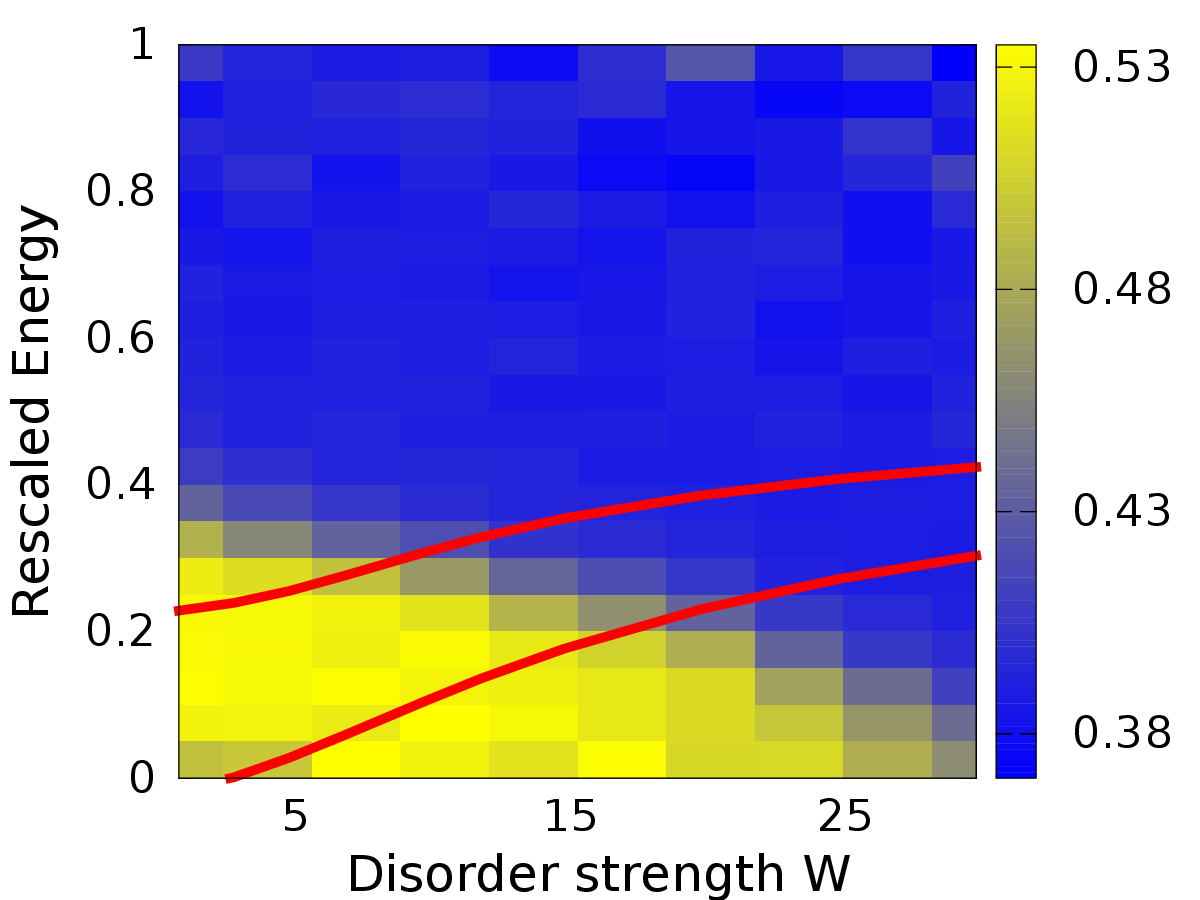
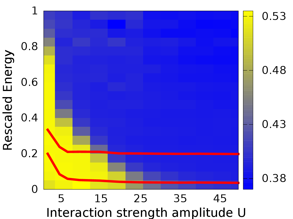
Figure 4: The mean ratio of consecutive spacing in the plane of disorder strength ($W$ or $U$ depending on the model) and rescaled energy $\epsilon=\frac{E-E_{bot}}{E_{top}-E_{bot}}$ with $N=12$ bosons on $L=8$ sites. Left panel - random chemical potential for $U=1$; middle panel - the same system for $U=5$; right panel - the random interactions case. Yellow color corresponds to $\overline{r}\approx 0.53$ and to the ergodic regime whereas the blue color denotes $\overline{r}\approx 0.39$ characteristic for localized states. Red curves indicate energies of the $|DW_{21}\rangle$ and $|DW_{30}\rangle$ states which cross the boundary between ergodic and localized regions of the spectrum with increasing disorder strength and exhibit ergodicity breaking.

The results are presented in Fig. 4. Clearly, all the systems reveal a transition between the ergodic phase (yellow color) with GOE-like $\overline{r}$ values and the localized (MBL) phase with statistics close to the Poisson limit. Typically, for a broad range of disorder strengths one may notice that, for a given disorder strength, high lying energy states are localized while the lowest remain extended. Thus, there exists an interval of energies (for a given disorder strength) where a transition from localized to extended states takes place. Such a behaviour is typically associated with the mobility edge for single-particle systems. Thus, we may loosely say that the apparent mobility edge is indeed observed for the studied systems. In both cases, it has a peculiar feature that states which are above a certain energy threshold are localized whereas the states below are extended, so it may be called an “inverted” mobility edge. This behavior has already been predicted for a two– and few–site bosonic systems in [55] with random on–site potentials.

While the transition between localized and extended states as a function of energy is clearly observed, it is by no means obvious that a sharp mobility edge exists in the thermodynamic limit. The properties of the transition regime (defined by the energy interval in which $\overline{r}$ takes intermediate values between Poisson and GOE limits) may be attributed to a mixture of localized and extended states for any finite size of the system or could stem from fractal properties of eigenstates. Another option is that the situation may be similar to the transition between chaotic and regular (integrable) motion in simple chaotic systems (see e.g. [56]) where “regular” states localized in the stable islands may coexist with chaotic eigenstates. In the deep semiclassical limit the residual tunnelings between regular islands and the chaotic sea decay exponentially (as $\hbar\rightarrow 0$) and regular and chaotic states may co-exist (leading e.g. to the so called Berry-Robnik statistics of levels [57]). The character of states in the transition regime is not known and whether the transition “sharpens” in the thermodynamic limit leading to a true mobility edge is an open question as the ergodic-MBL transition is claimed to be dynamical in nature [38]. Also, the disorder is known to smear the transition due to the presence of Griffiths regions [40].

We observe that regions of extended (yellow) and localized (blue) behavior have different shapes depending on the model as well as on the parameters – see Fig 4. The left ($U=1$) and middle ($U=5$) panels correspond to the random on-site potential model. For stronger interactions extended states are limited to the lower part of the energy spectrum. High energy states, necessarily having significant occupations on selected sites, are localized even for very small disorder. This difference in shape for different strengths of interactions nicely correlates with different temporal behaviors of the $|DW_{21}\rangle$ and $|DW_{30}\rangle$ imbalances. The energies of these states are represented by red lines in all three panels of Fig 4. They are quite similar during the transition from the extended to the localized regime in the left panel ($U=1$), thus they should have a similar stationary imbalance. Indeed, this is the case as shown in the left panel of Fig. 3. For stronger interactions, the two red lines enter the localized (blue) region for different disorder strengths – as faithfully reproduced by the the disorder dependence of stationary imbalance (middle panel in Fig. 3). Similar correlation is observed for the random interactions model (right panels of Fig 4 and Fig. 3).

In the next section we provide perturbative arguments backing our conclusion on observation of the apparent inverted mobility edge.

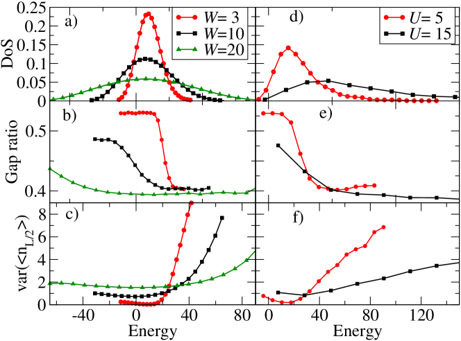
Figure 5: Density of states – panels a) and d), mean ratio of consecutive spacings $\overline{r}$ as function of energy – panels b) and e) and the variance of the occupation of the central $L/2$ site $\mathrm{var}(\langle n_{L/2}\rangle)$ as function of energy – panels c) and f) for the models with random chemical potential and $U=1$ (left column) and for random interactions (right column). The disorder amplitudes are given in the figure. A system of $N=9$ bosons in $L=6$ lattice sites (500 realizations averaged) is analyzed.

4 Interactions as a perturbation

The perturbative work [8] established the existence of many–body localization for a system of interacting fermions and the results were extended to MBL of bosons [58]. The key element is the ratio, ${\cal R}$, of the matrix element between two states localized at different sites to the difference in their energies. The ratio larger than unity leads to delocalization, whereas the states remain localized for a small ${\cal R}$. This argument, used originally for discussing Anderson transition, may be applied also to MBL. It also lies at the heart of the renormalization group treatment of MBL transition [36, 37].

It is straightforward to adapt this reasoning to the system with random on–site potential (1). At $U=0$, it reduces to Anderson model – working in its single particle localized basis, we assume the localization/delocalization transition happens when the energy mismatch between energies of initial states $\epsilon_{i},\,\epsilon_{j}$ and final states $\epsilon_{k},\,\epsilon_{l}$ becomes comparable with the coupling $U_{ij,kl}$ between those states which stems from the on–site interaction term in the Hamiltonian (1), so that

$${{\cal R}=U_{ij,kl}/|\epsilon_{i}+\epsilon_{j}-\epsilon_{l}-\epsilon_{k}|\approx 1.}$$ (5)

The annihilation operator, $a_{i}$, associated with the Wannier basis state on site $i$ can be written as a combination of operators annihilating particles in single–particle localized states, $b_{j}$

$${a_{i}=\sum_{j}\varphi^{j}_{i}b_{j},}$$ (6)

where the coefficients $\varphi^{j}_{i}$ decay exponentially with the distance between sites $i$ and $j$. Now, the single–particle part of (2) can be written as

$${H_{0}=\sum_{j}\epsilon_{j}b^{{\dagger}}_{j}b_{j}}$$ (7)

and the interaction part becomes

$${H_{1}=\frac{1}{2}U\sum_{i,j_{1},j_{2},j_{3},j_{4}}\varphi^{j_{1}}_{i}\varphi^{j_{2}}_{i}\varphi^{j_{3}}_{i}\varphi^{j_{4}}_{i}b^{{\dagger}}_{j_{1}}b^{{\dagger}}_{j_{2}}b_{j_{3}}b_{j_{4}}.}$$ (8)

The exponential decay of $\varphi^{j}_{i}$ with the distance $|i-j|$ implies that the terms in (8) can be organized order by order considering the index sum $S=|j-j_{1}|+|j-j_{2}|+|j-j_{3}|+|j-j_{4}|$. The zero order term $S=0$ reads $\frac{1}{2}U\sum_{i}(\varphi^{i}_{i})^{4}n^{b}_{i}(n^{b}_{i}-1)$ and corresponds to a mere shift of energies of the eigenstates of the system due to the interactions. The first order terms $S=1$ are of the form of the density–induced tunnelings $b^{{\dagger}}_{i}n^{b}_{i}b_{i+1}$ and are smaller than the $S=0$ terms by a factor $\varphi^{i+1}_{i}/\varphi^{i}_{i}$. This classification may be continued to higher order terms.

The question is whether the condition (5) together with the form of the interaction–induced terms can be used to get some qualitative understanding of the observed ergodic to MBL transition in the interacting system. Consider the system with random a on–site potential and its density of states (DoS) – Fig. 5a. At high energies, the density of states is small, therefore, the energy mismatches between the states that can be coupled by the interaction (8) are sufficiently large for the system to remain localized even in the presence of interactions. Consequently $\overline{r}\approx 0.4$ in that region of the spectrum – Fig. 5b. Now, as the energy decreases, the DoS grows larger and the energy differences between states coupled by the off-diagonal part of (8) become comparable with the coupling. For $W=3$, states in this part of the spectrum are ergodic – $\overline{r}\approx 0.53$. On the other hand, for $W=10$, the coupling is not strong enough, $\overline{r}\approx 0.45$ and the system is in the intermediate regime.

However, at the smallest energies, the DoS is low again – so why the does system remain ergodic (or closer to the ergodic phase) even though the energy mismatches seem to be bigger again? First, let us note, that the DoS is slightly asymmetric due to the quadratic nature of the interaction term. Consider a state at the bottom of the spectrum – it necessarily has large occupations of single–particle orbitals localized around sites with a large negative chemical potential. The $S=0$ term $n^{b}_{i}(n^{b}_{i}-1)$ shifts energy of this state upwards, to a region of spectrum where the DoS is higher. Now consider a state at the top of the spectrum, its energy is again increased by the interactions but now the state is shifted towards the high end of the spectrum, where the DoS is low. Therefore, the $S=0$ term is the first source of an asymmetry between lower and higher parts of the spectrum. However, the differences between eigenstates in those regions are much more pronounced which is well captured by $\mathrm{var}(\langle n_{L/2}\rangle)$ – variance (with respect to different disorder realizations) of the average occupation of the central site of the lattice, which is shown in Fig. 5c. The $\mathrm{var}(\langle n_{L/2}\rangle)$ increases rapidly at large energies and renders the system localized. Conversely, at low energies, fluctuations of the number of the particles are smaller and the interactions delocalize the eigenstates easily.

The system with random interactions – see the Fig. 5d-f is not straightforwardly treatable with the same perturbative analysis as the single–particle physics at $U=0$ is delocalized. However, the general results of the reasoning for the random chemical potential are the same - the DoS is much more asymmetric and states at high energies are localized. Moreover, $\mathrm{var}(\langle n_{L/2}\rangle)$ looks quantitatively the same and shows that also for the random interactions states at the lower parts of spectrum have a better chance of being ergodic.

Concluding, the inverted localization character of states (with low energy states being extended and high energy states tending to be localized) in the Bose–Hubbard model stems from the possible higher than one occupation of lattice sites ($\mathrm{var}(\langle n_{L/2}\rangle)>1$) and the fact that the interaction energy increases quadratically with the site occupation.

5 Level statistics

The spectral statistics are a useful probe of the MBL transition which we have already seen in Sec. 3 discussing the gap ratio. Let us now concentrate on a more traditional level statistics, the distribution of spacings. A generic ergodic system is characterized by Wigner-Dyson statistics characteristic for GOE matrices, whereas for an integrable system (i.e. also in the MBL phase where a complete set of LIOMs exists [52, 9, 53]) the Poissonian statistics is appropriate [56]. The intermediate statistics in the context of ergodic to many–body localized transition is addressed in [59] on an example of a Heisenberg $XXZ$ spin chain. Serbyn and Moore postulated that the transition might be described by the so called plasma model [59]. More precisely, using a random walk approach in a space of Hamiltonians generated by different realizations of disorder [60], with mean field based assumptions on the correlation functions for these Hamiltonians, as well as assuming fractal scaling to the matrix elements of local operators Serbyn and Moore obtain a power law scaling for the disorder inducing term of the Hamiltonian (they explicitly consider XXZ spin model). This allows them, in turn, to map their model onto the plasma model for level statistics [61]. The model predicts the level spacing distribution $P(s)$ for large $s$ that interpolates between the exponential and the Gaussian tail. Assuming also a plausible power law repulsion at small spacings, one arrives at [59]

$$P(s)\propto s^{\beta}\mathrm{e}^{-C_{\gamma,\beta}s^{2-\gamma}}$$ (9)

with $\beta$ and $\gamma$ being the parameters of the plasma model. It is shown to well describe the level spacing distribution for the studied spin system across the transition.

Level spacing distributions were also used by us [18] for randomly interacting bosons to estimate the position of the critical region between the ergodic and localized phases. We found that the distribution of spacings was well described by the plasma model distribution between GOE and Poisson limits. In fact, we have identified two regimes; the generalized semi-Poisson [62] regime close to the MBL phase corresponding to $\gamma=1$ and variable $\beta$ followed by the transition to GOE for $\beta=1$ and $\gamma$ decreasing to zero. In the following, we discuss mainly the spacing distribution for the random chemical potential model (1) and make some comments on the random interactions model.

After performing the necessary unfolding of energy levels [56] we obtain the distribution of spacings between neighboring energy levels $P(s)$ with the mean level spacing equal to unity - the results for a a random chemical potential are presented in Fig. 6. The level spacing $P(s)$ at small disorder ($W=1$) is well approximated by the Wigner’s surmise [63] $P(s)=\frac{\pi}{2}s\mathrm{e}^{-\frac{\pi}{4}s^{2}}$ which confirms the ergodic behavior of the system. At large values of disorder ($W=25$), deep in the MBL phase, the system is fully integrable [52, 9], and the resulting spacing distribution is Poissonian $P(s)=\mathrm{e}^{-s}$.

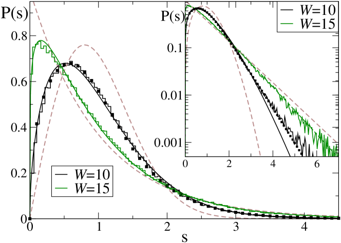
Figure 6: Level spacings distributions for the system with random chemical potential for $N=12$ bosons on $L=8$ sites with $U=1$. Data for $W=1$ and $W=30$ are well reproduced by the Wigner’s surmise formula and Poisonian statistics (brown dashed lines) and are not displayed to ensure better visibility of data for $W=10,15$. Those are fitted with the plasma model distribution and semi–Poissonian statistics respectively (solid lines). Finally, the squares correspond to our effective formula (10). The inset presents the same data in the lin-log scale showing that the plasma model fails to reproduce the exponential tail of the numerical data despite a seemingly good fit of the bulk (main panel).

It is notable that the transition between the two limiting distributions follows the similar pattern to that observed before [59, 18]. In the transition region, we observe a two stage process as in [18]. However, at smaller values of disorder we find out, quite surprisingly, that the proposed plasma model [59], while nicely reproducing the bulk of the distribution for $W=10$ – see Fig. 6, does not reproduce our data well in the tail of the distribution, as shown in the inset of Fig. 6. For fitted values of $\beta$ and $\gamma$ the plasma model distribution decays faster than exponentially $\gamma=0.59<1$ while the numerically obtained data reveal an exponential tail. Forcing $\gamma=1$ to get the agreement in the tail leads to a poor comparison of numerics and plasma model distribution for small and moderate spacings. To resolve this issue we fit the data for $W=10$ with the formula

$$P(s)=s^{\beta}(C_{1}+C_{2}\mathrm{Erf}(C_{3}(s-s_{0}))\mathrm{e}^{-\alpha s},$$ (10)

in such a way, that $\beta$ and $\alpha$ are fixed by the limiting behavior of $P(s)$ at small and large $s$, respectively, two of the $C_{1,2,3}$ constants are fixed by the requirement that $\langle 1\rangle=1=\langle s\rangle$ and the remaining one and $s_{0}$ are fitted. The fit of (10) reproduces both the tail and the bulk of the level spacing distribution more accurately than the plasma model prediction. Let us stress, that the formula (10) is not a result of a deeper theory, but rather a heuristic formula which grasps effectively all essential features of the level spacing distribution.

The deviation from the plasma model occurs close to the delocalized regime. Importantly, after a close inspection, we have observed exactly the same behavior for the model with random interactions. While the distribution of the bulk (small or intermediate $s$) of the spacing distribution was well captured by the plasma model as reported by us [18], the large spacing tail remained exponential and the fits with the proposed distribution (10) were clearly superior (since the data resemble that of Fig. 6 we do not reproduce them).

At larger disorder strengths, level spacing distributions of both considered systems (1), (2) are well described by the generalized semi–Poison distribution $P(s)\propto s^{\beta}\mathrm{e}^{-(\beta+1)s}$.

Concluding, the level statistics for the Bose–Hubbard model with random on–site chemical potential or with random interactions reveal the ergodic to MBL transition and the level spacings distributions in the intermediate regime are similar to XXZ–Heisenberg spin chain [59]. However, the 2-parameter plasma model is insufficient to capture the level spacings in the critical regime close to the ergodic phase (as for $W=10$) because of the exponentially decaying tails of numerically obtained $P(s)$.

6 Fate of metastable states in presence of disorder

The previous sections demonstrate that the disordered Bose–Hubbard models possess the characteristic features of MBL systems. In particular, following the time evolution of the initial density–wave states one observes ergodicity breaking. However, it has been shown that [26] strong repulsive interactions of bosons lead to dynamical constraints which slow down thermalization of the system as soon as it is prepared in a highly excited inhomogeneous initial state. In this section, we compare this mechanism to the disorder induced ergodicity breaking.

The overall thermalization rate of the clean system depends on the population of high–energy excitations, which, at strong interactions, is associated with states having sites occupied by more than a single boson.

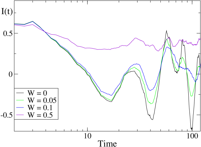
Figure 7: (color online) $I(t)$ for various disorder strengths (averaged over $30$ disorder realizations) for $N=8$ bosons on $L=8$ sites at $U=10$. With growing disorder strength, the oscillations amplitude gets smaller and a non–zero average value of imbalance is obtained – already relatively small disorder $W=0.5$ leads to significant ergodicity breaking and $I_{stat}\approx 0.36$.

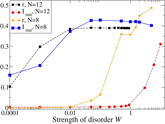
Figure 8: Change in $\bar{r}$ and stationary value of imbalance resulting from introducing disorder to the system. At small $W$ the $\overline{r}$ value is smaller than value characteristic for uncorrelated Poissonian energy levels – once $\bar{r}\approx 0.4$ is attained, non–zero stationary value of imbalance is observed and the system is no longer ergodic. The parameters are $U=20$ for $N=12$ and $U=10$ for $N=8$.

For instance, doublons from the density–wave state $|DW_{20}\rangle$ (at filling $\nu=1$) very slowly decay at large $U$ being incapable of moving and restoring translational symmetry. That was quantified in [26] by the relaxation time $\tau_{R}$ - the smallest time at which the local density acquires its equilibrium value. $\tau_{R}$ was found to be increasing with the interaction strength and with the growing system size.

In order to demonstrate that the dynamical trapping described above and MBL induced by disorder are two physically distinct phenomena, we consider a system of $N=8$ bosons on $L=8$ sites with strong interactions $U=10$ and gradually increase disorder strength $W$. The relaxation time of the system is $\tau_{R}\approx 10$. After this time $I(t)$ oscillates around zero and the system thermalizes. The imbalance $I(t)$ calculated for different disorder strengths is presented in Fig. 7. Clearly, even though the time evolution at small times is similar for different , and hence $\tau_{R}$ does not change drastically in the interval $W\in[0,0.3]$, the long time evolution is affected – the oscillations of $I(t)$ (disorder averaged) are smaller and already for $W=0.1$ a non–zero stationary value of imbalance builds up. The dependence of stationary values of imbalance on the disorder strength together with the corresponding $\overline{r}$ values are presented in Fig. 8. Clearly, at larger $W$ a non–zero stationary value of imbalance is observed, moreover it happens only at disorder strengths that correspond to $\bar{r}\approx 0.4$ – i.e in the MBL regime.

Therefore, for very small disorder strengths the slow down of relaxation due to metastable states at large $U$ prevails. However, an addition of even a small disorder to this strongly interacting system affects its dynamics severely and leads to a much more robust mechanism of ergodicity breaking.

7 Conclusions

We have presented a comprehensive analysis of many-body localization for a system of interacting bosons in a lattice in the presence of disorder. We considered both the random chemical potential as well as we revisited the case of random interactions. Both systems can be realized experimentally in optical lattices.

The treatment of interacting bosons in a lattice is technically more difficult than spin=1/2 or fermionic systems due to the possibility of multiple occupations of individual sites. This, in principle could lead to profound differences w.r.t. fermions/spins as the local Hilbert space might be viewed as an additional synthetic dimension. However, as found above, the repulsive interactions between bosons limit multiple occupancies to uninteresting high energy physics. For the majority of states, at the intermediate energies the character of MBL observed is similar to that of spins and fermions. In particular, MBL may be evidenced by a long-time behavior of the imbalance of appropriately prepared inhomogeneous initial states. In this respect bosonic physics is richer, allowing for a preparation of different states, possibly differing in energy. This may allow one to experimentally study the energy dependence of the transition between ergodic and MBL phases when the disorder is increased. This is particularly interesting as we have shown that the system reveals an apparent localization (mobility) edge. Moreover this “edge” is inverted in a sense that localized states lay higher in energy than the extended ergodic states that occupy lower energy sector. Let us stress that it is the bosonic nature of the models which allows for initial density wave states at significantly different energies. An experiment in which the time evolution of the imbalance starting from the $|DW_{21}\rangle$ and $|DW_{30}\rangle$ density–wave states would verify the existence of the apparent mobility edges.

In the critical quantum regime between ergodic and localized phases (in our necessarily finite size systems studies) we observe an algebraic decay of the imbalance in agreement with the subdiffusive character predicted in a general one-dimensional renormalization group theory [36, 37].

In the case of the revisited random interactions, the thorough investigation of the critical region characterized by subdiffusion for small system sizes leads us to a better estimation of the stationary imbalance. The results about the mobility edge are confirmed for larger system size. The direct comparison with the random on–site potential model allows us to speculate that the underlying mechanism of MBL is similar in both systems.

The detailed analysis of level spacing distributions in the transition regime revealed that the so called plasma model [59] fails to reproduce the behavior of the tail of the distribution despite faithfully reproducing the bulk. On the other hand the similarity of spin and boson level statistics in the transition regime suggests a significant level of universality in the transition between ergodic - many-body localized phases and calls for a separate analysis. Such an analysis is in progress.

8 Acknowledgement

We are grateful to Dominique Delande for illuminating discussions throughout the course of this work. We acknowledge also useful conversations with Fabian Alet and Antonello Scardicchio. We thank Jesse Mumford for reading and correcting the grammar in the manuscript. This research was performed within project No.2015/19/B/ST2/01028 financed by National Science Centre (Poland). Support by PL-Grid Infrastructure and by EU via project QUIC (H2020-FETPROACT-2014 No. 641122) is also acknowledged.

9 References

References

- [1] Anderson P W 1958 Phys. Rev. 109 1492
- [2] Altshuler B L and Aronov A G 1979 Solid State Commun. 30 115
- [3] Altshuler B L, Aronov A G and Lee P A 1980 Phys. Rev. Lett. 44 1288
- [4] Fukuyama H 1980 J. Phys. Soc. Jpn. 48 2169
- [5] Fleishman L and Anderson P W 1980 Phys. Rev. B 21(6) 2366–2377 https://link.aps.org/doi/10.1103/PhysRevB.21.2366
- [6] Shepelyansky D L 1994 Phys. Rev. Lett. 73 2607
- [7] Damski B, Zakrzewski J, Santos L, Zoller P and Lewenstein M 2003 Phys. Rev. Lett. 91 080403
- [8] Basko D, Aleiner I and Altschuler B 2006 Ann. Phys. (NY) 321 1126
- [9] Huse D A, Nandkishore R and Oganesyan V 2014 Phys. Rev. B 90(17) 174202 http://link.aps.org/doi/10.1103/PhysRevB.90.174202
- [10] Nandkishore R and Huse D A 2015 Ann. Rev. Cond. Mat. Phys. 6 15
- [11] Abanin D A and Papić Z 2017 Annalen der Physik 529 1700169 1700169 http://dx.doi.org/10.1002/andp.201700169
- [12] Alet F and Laflorencie N 2017 ArXiv e-prints: 1711.03145
- [13] Schreiber M, Hodgman S S, Bordia P, Lüschen H P, Fischer M H, Vosk R, Altman E, Schneider U and Bloch I 2015 Science 349 7432
- [14] Kondov S S, McGehee W R, Xu W and DeMarco B 2015 Phys. Rev. Lett. 114(8) 083002 https://link.aps.org/doi/10.1103/PhysRevLett.114.083002
- [15] White M, Pasienski M, McKay D, Zhou S Q, Ceperley D and DeMarco B 2009 Phys. Rev. Lett. 102(5) 055301 https://link.aps.org/doi/10.1103/PhysRevLett.102.055301
- [16] Choi J y, Hild S, Zeiher J, Schauß P, Rubio-Abadal A, Yefsah T, Khemani V, Huse D A, Bloch I and Gross C 2016 Science 352 1547–1552
- [17] Tang B, Iyer D and Rigol M 2015 Phys. Rev. B 91(16) 161109 http://link.aps.org/doi/10.1103/PhysRevB.91.161109
- [18] Sierant P, Delande D and Zakrzewski J 2017 Phys. Rev. A 95(2) 021601 https://link.aps.org/doi/10.1103/PhysRevA.95.021601
- [19] Sierant P, Delande D and Zakrzewski J 2017 Acta Phy. Polon. B in press xxxx https://arxiv.org/abs/1707.08845
- [20] Zhou S Q and Ceperley D M 2010 Phys. Rev. A 81(1) 013402 https://link.aps.org/doi/10.1103/PhysRevA.81.013402
- [21] Bakr W S, Gillen J I, Peng A, Fölling S and Greiner M 2009 Nature 462 74–77 http://dx.doi.org/10.1038/nature08482
- [22] Gimperlein H, Wessel S, Schmiedmayer J and Santos L 2005 Phys. Rev. Lett. 95 170401
- [23] Lüschen H P, Bordia P, Scherg S, Alet F, Altman E, Schneider U and Bloch I 2017 Phys. Rev. Lett. 119(26) 260401 https://link.aps.org/doi/10.1103/PhysRevLett.119.260401
- [24] Ancilotto F, Rossini D and Pilati S 2018 ArXiv e-prints (Preprint 1801.05596)
- [25] Zakrzewski J and Delande D 2018 ArXiv e-prints (Preprint 1802.02525)
- [26] Carleo G, Becca F, Schiro M and Fabrizion M 2012 Scientific Reports 2(243) http://dx.doi.org/10.1038/srep00243
- [27] Deutsch J M 1991 Phys. Rev. A 43(4) 2046–2049 https://link.aps.org/doi/10.1103/PhysRevA.43.2046
- [28] Srednicki M 1994 Phys. Rev. E 50(2) 888–901 https://link.aps.org/doi/10.1103/PhysRevE.50.888
- [29] Cohen D, Yukalov V I and Ziegler K 2016 Phys. Rev. A 93(4) 042101 https://link.aps.org/doi/10.1103/PhysRevA.93.042101
- [30] Luitz D J, Laflorencie N and Alet F 2015 Phys. Rev. B 91(8) 081103 https://link.aps.org/doi/10.1103/PhysRevB.91.081103
- [31] Luitz D J, Laflorencie N and Alet F 2016 Phys. Rev. B 93(6) 060201 http://link.aps.org/doi/10.1103/PhysRevB.93.060201
- [32] Jun Park T and Light J 1986 J. Chem. Phys. 85 5870–5876
- [33] Agarwal K, Gopalakrishnan S, Knap M, Müller M and Demler E 2015 Phys. Rev. Lett. 114(16) 160401 https://link.aps.org/doi/10.1103/PhysRevLett.114.160401
- [34] Bar Lev Y, Cohen G and Reichman D R 2015 Phys. Rev. Lett. 114(10) 100601 https://link.aps.org/doi/10.1103/PhysRevLett.114.100601
- [35] Torres-Herrera E J and Santos L F 2015 Phys. Rev. B 92(1) 014208 https://link.aps.org/doi/10.1103/PhysRevB.92.014208
- [36] Vosk R, Huse D A and Altman E 2015 Phys. Rev. X 5(3) 031032 https://link.aps.org/doi/10.1103/PhysRevX.5.031032
- [37] Potter A C, Vasseur R and Parameswaran S A 2015 Phys. Rev. X 5(3) 031033 https://link.aps.org/doi/10.1103/PhysRevX.5.031033
- [38] Khemani V, Lim S P, Sheng D N and Huse D A 2017 Phys. Rev. X 7(2) 021013 https://link.aps.org/doi/10.1103/PhysRevX.7.021013
- [39] Griffiths R B 1969 Phys. Rev. Lett. 23(1) 17–19 https://link.aps.org/doi/10.1103/PhysRevLett.23.17
- [40] Vojta T 2010 J. Low Temp. Phys. 161 299–323
- [41] Agarwal K, Altman E, Demler E, Gopalakrishnan S, A Huse D and Knap M 2017 Annalen der Physik 529 201600326
- [42] Vidal G 2003 Phys. Rev. Lett. 91(14) 147902 http://link.aps.org/doi/10.1103/PhysRevLett.91.147902
- [43] Vidal G 2004 Phys. Rev. Lett. 93(4) 040502 http://link.aps.org/doi/10.1103/PhysRevLett.93.040502
- [44] Zakrzewski J and Delande D 2009 Phys. Rev. A 80(1) 013602 http://link.aps.org/doi/10.1103/PhysRevA.80.013602
- [45] Schollwoeck 2011 Ann. Phys. (NY) 326 96
- [46] Serbyn M, Papić Z and Abanin D A 2013 Phys. Rev. Lett. 110(26) 260601 http://link.aps.org/doi/10.1103/PhysRevLett.110.260601
- [47] Mott N F 1990 Metal-Insulator Transitions, 2nd Edition (Taylor and Francis Ltd., London)
- [48] Naldesi P, Ercolessi E and Roscilde T 2016 SciPost Phys. 1(1) 010 https://scipost.org/10.21468/SciPostPhys.1.1.010
- [49] Lin S H, Sbierski B, Dorfner F, Karrasch C and Heidrich-Meisner F 2017 ArXiv e-prints 1707.06759
- [50] Oganesyan V and Huse D A 2007 Phys. Rev. B 75(15) 155111 http://link.aps.org/doi/10.1103/PhysRevB.75.155111
- [51] Atas Y Y, Bogomolny E, Giraud O and Roux G 2013 Phys. Rev. Lett. 110(8) 084101 http://link.aps.org/doi/10.1103/PhysRevLett.110.084101
- [52] Serbyn M, Papić Z and Abanin D A 2013 Phys. Rev. Lett. 111(12) 127201 http://link.aps.org/doi/10.1103/PhysRevLett.111.127201
- [53] Imbrie J Z, Ros V and Scardicchio A 2017 Annalen der Physik 529 201600278
- [54] Pal A and Huse D A 2010 Phys. Rev. B 82(17) 174411 http://link.aps.org/doi/10.1103/PhysRevB.82.174411
- [55] Singh R and Shimshoni E 2017 Annalen der Physik 529 1600309 http://dx.doi.org/10.1002/andp.201600309
- [56] Haake F 2010 Quantum Signatures of Chaos (Springer, Berlin)
- [57] Prosen T and Robnik M 1994 Journal of Physics A: Mathematical and General 27 L459 http://stacks.iop.org/0305-4470/27/i=13/a=001
- [58] Aleiner I L, Altshuler B L and Shlyapnikov G V 2010 Nat Phys 6 900–904 http://dx.doi.org/10.1038/nphys1758
- [59] Serbyn M and Moore J E 2016 Phys. Rev. B 93(4) 041424 http://link.aps.org/doi/10.1103/PhysRevB.93.041424
- [60] Chalker J T, Lerner I V and Smith R A 1996 Phys. Rev. Lett. 77(3) 554–557 https://link.aps.org/doi/10.1103/PhysRevLett.77.554
- [61] Kravtsov V E and Lerner I 1995 J. Phys. A: Math. Gen. 28 3623
- [62] Bogomolny E B, Gerland U and Schmit C 1999 Phys. Rev. E 59(2) R1315–R1318 https://link.aps.org/doi/10.1103/PhysRevE.59.R1315
- [63] Bohigas O, Giannoni M J and Schmit C 1984 Phys. Rev. Lett. 52(1) 1–4 https://link.aps.org/doi/10.1103/PhysRevLett.52.1