Multiscale computational method for heat conduction problems of composite structures with diverse periodic configurations in different subdomains

Abstract

This study develops a novel multiscale computational method for heat conduction problems of composite structures with diverse periodic configurations in different subdomains. Firstly, the second-order two-scale (SOTS) solutions for these multiscale problems are successfully obtained based on asymptotic homogenization method. Then, the error analysis in the pointwise sense is given to illustrate the importance of developing SOTS solutions. Furthermore, the error estimates for the SOTS approximate solutions in the integral sense is presented. In addition, a SOTS numerical algorithm is proposed to effectively solve these problems based on finite element method. Finally, some numerical examples verify the feasibility and effectiveness of the SOTS numerical algorithm we proposed.

1 Introduction

With the rapid development of material science and technology, composite materials are widely used in aeronautic and aerospace engineering owing to their excellent physical properties. These composites usually serve under complex and extreme heat environments. In practical engineering application, engineers and designers always adopt diverse composites in different subdomains of a whole engineering structure for creating the more complex components and systems. In order to obtain the optimal design of engineering structures, it is significant to accurately evaluate and predict the thermal responses of the composites. It is well-known that the complexity and heterogeneity (inclusions or holes) of composite materials often cause costly computational efforts [1, 2, 3, 4, 5, 6]. Fortunately, in the last thirty years, mathematicians and engineers have developed some multiscale methods to solve this difficult problem, such as the asymptotic homogenization method (AHM), heterogeneous multiscale method (HMM), variational multiscale method (VMS), multiscale finite element method (MsFEM) and multiscale eigenelement method (MEM), etc [7, 8]. As far as we know, many studies were performed on heat conduction problems of the composites. However, most of these studies focused on heat conduction problems of engineering structures manufactured by the same composites in the whole structures [1, 2, 3, 4, 5, 6]. To the best of our knowledge, there is a lack of adequate researches on heat conduction problems of composite structures with diverse periodic configurations in different subdomains [9, 10].

The aim of this paper is to develop a multiscale computational method to effectively solve the heat conduction problems of composite structures with diverse periodic configurations in different subdomains. Based on the asymptotic homogenization method, we establish a novel SOTS analysis method and associated numerical algorithm for the above-mentioned multiscale problems.

This paper is outlined as follows. In Section 2, the detailed construction of the SOTS solutions for heat conduction problems of composite structures with diverse periodic configurations in different subdomains is given by multiscale asymptotic analysis. In Section 3, the error analysis in the pointwise sense of first-order two-scale (FOTS) solutions and SOTS solutions is obtained. By comparing the results of error analysis of FOTS solutions and SOTS solutions in the pointwise sense, we theoretically explain the importance of SOTS solutions in capturing micro-scale information. Moreover, an explicit convergence rate for the SOTS solutions are derived under some hypotheses. In Section 4, a SOTS numerical algorithm based on FEM and FDM is presented to effectively solve these multiscale problems. In Section 5, some numerical results are shown to verify the validity of our SOTS algorithm. Finally, some conclusions are given in Section 6.

For convenience, throughout the paper we use the Einstein summation convention on repeated indices.

2 SOTS analysis of the governing equation

Let us consider the following governing equation for heat conduction problems of composite structures with diverse periodic configurations in different subdomains

$$\left\{\begin{aligned} &-\frac{\partial}{\partial{x_{i}}}\Big{(}{k_{ij}^{\bm{\varepsilon}}({\mathbf{x}})\frac{\partial T^{\bm{\varepsilon}}(\mathbf{x})}{\partial{x_{j}}}}\Big{)}=h(\mathbf{x}),\;\;\text{in}\;\;\Omega=\bigcup\limits_{s=1}^{K}{\Omega_{s}},\;\;\bm{\varepsilon}=(\varepsilon_{1},\cdots\varepsilon_{K}),\\ &T^{\bm{\varepsilon}}(\mathbf{x})=\widehat{T}(\mathbf{x})\;\;\;\text{on}\;\;\partial{\Omega_{T}},\\ &{k_{ij}^{\bm{\varepsilon}}({\mathbf{x}})\frac{\partial T^{\bm{\varepsilon}}(\mathbf{x})}{\partial{x_{j}}}}{n_{i}}=\bar{q}(\mathbf{x})\;\;\;\text{on}\;\;\partial{\Omega_{q}}\end{aligned}\right.$$ (1)

where $\Omega$ is a bounded convex domain in $\mathbb{R}^{\mathcal{N}}(\mathcal{N}=2,3)$ with a boundary $\partial\Omega=\partial\Omega_{T}\cup\partial\Omega_{q}$; $\Omega_{s}$ denotes a component, that is made of composite materials with periodic configuration $C_{s}$ and characteristic periodic size $\varepsilon_{s}$; $T^{\bm{\varepsilon}}(\mathbf{x})$ are undetermined temperature field; $k_{ij}^{\bm{\varepsilon}}({\mathbf{x}})$ is the second order thermal conductivity tensor; $h(\mathbf{x})$ is the internal heat source; $\widehat{T}({\bf{x}})$ is the prescribed temperature on the boundary $\partial\Omega_{T}$; $\bar{q}({\bf{x}})$ is the heat flux prescribed normal to the boundary $\partial\Omega_{q}$ with the normal vector $n_{i}$.

To begin with, let us set $\displaystyle\mathbf{y}^{s}=\frac{\mathbf{x}}{\varepsilon_{s}}$ for $\mathbf{x}\in\Omega_{s}$ as micro-scale coordinates of periodic unit cell $Q^{s}=(0,1)^{\mathcal{N}}$. With this notation, we have the following chain rule

$$\frac{\partial}{\partial x_{i}}\rightarrow\frac{\partial}{\partial x_{i}}+\frac{1}{\varepsilon_{s}}\frac{\partial}{\partial y_{i}^{s}},\;\;\mathbf{x}\in\Omega_{s}$$ (2)

which will be extensively used in the sequel. Hence, $k_{ij}^{\bm{\varepsilon}}({\mathbf{x}})$ can be changed into $k_{ij}({\mathbf{y}}^{s})$ for $\mathbf{x}\in\Omega_{s}$. Being similar to [3, 4, 5, 6], we make the following assumptions:

1. $k_{ij}({\mathbf{y}}^{s})$ is a scalar function belonging to $L^{\infty}(\Omega)$ and function $k_{ij}({\mathbf{y}}^{s})$ is $1-$periodic (with $Q^{s}=(0,1)^{\mathcal{N}}$) for $\mathbf{x}\in\Omega_{s}$.

2. functions $k_{ij}({\mathbf{y}}^{s})$ is symmetric and there exist two constants $0<\gamma_{0}\leq\gamma_{1}$ such that

   $$\gamma_{0}|\bm{\xi}|^{2}\leq k_{ij}^{\bm{\varepsilon}}({\mathbf{x}})\xi_{i}\xi_{j}\leq\gamma_{1}|\bm{\xi}|^{2},\;\;\mathbf{x}\in\Omega$$

   for all vectors $\bm{\xi}=(\xi_{i})\in\mathbb{R}^{\mathcal{N}}$ and all symmetric matrix $\{\eta_{ij}\}\in\mathbb{R}^{\mathcal{N}}\times\mathbb{R}^{\mathcal{N}}$.

3. $h(\mathbf{x})\in L^{2}(\Omega),\widehat{T}(\mathbf{x})\in L^{2}(\Omega),\bar{q}(\mathbf{x})\in L^{2}(\Omega)$.

Now, we give the specific construction process of the FOTS solution and SOTS solution for problem (1). To the problem (1), we assume that $T^{\bm{\varepsilon}}(\mathbf{x})$ can be formally expanded as follows:

$$T^{\bm{\varepsilon}}(\mathbf{x})={T^{(0)}}(\mathbf{x},\mathbf{y}^{s})+\varepsilon_{s}{T^{(1)}}(\mathbf{x},\mathbf{y}^{s})+{\varepsilon_{s}^{2}}{T^{(2)}}(\mathbf{x},\mathbf{y}^{s})+{\rm O}({\varepsilon_{s}^{3}}),\;\;\mathbf{x}\in\Omega_{s}$$ (3)

Substituting (3) into (1) and by virtue of the chain rule (2), we have

$$-\varepsilon_{s}^{-2}\frac{\partial}{\partial y_{i}^{s}}\Big{(}{{k_{ij}}({\bf{y}}^{s})\frac{\partial T^{(0)}}{\partial y_{j}^{s}}}\Big{)}-\varepsilon_{s}^{-1}\frac{\partial}{\partial y_{i}^{s}}\Big{(}{k_{ij}({\bf{y}}^{s})\big{(}{\frac{\partial T^{(0)}}{\partial{x_{j}}}+\frac{\partial T^{(1)}}{\partial y_{j}^{s}}}\big{)}}\Big{)}$$ (4)

$$-\varepsilon_{s}^{-1}\frac{\partial}{\partial{x_{i}}}\Big{(}{k_{ij}({\bf{y}}^{s})\frac{\partial{T^{(0)}}}{\partial y_{j}^{s}}}\Big{)}-\varepsilon_{s}^{0}\frac{\partial}{\partial y_{i}^{s}}\Big{(}{k_{ij}({\bf{y}}^{s})\big{(}{\frac{\partial{T^{(1)}}}{\partial{x_{j}}}+\frac{\partial{T^{(2)}}}{\partial y_{j}^{s}}}\big{)}}\Big{)}$$

$$-\varepsilon_{s}^{0}\frac{\partial}{\partial{x_{i}}}\Big{(}{k_{ij}({\bf{y}}^{s})\big{(}{\frac{\partial{T^{(0)}}}{\partial{x_{j}}}+\frac{\partial{T^{(1)}}}{\partial y_{j}^{s}}}\big{)}}\Big{)}+O({\varepsilon_{s}})=h,\;\;\mathbf{x}\in\Omega_{s}$$

From (4), a series of equations in $\Omega_{s}$ are derived by matching terms of the same order of $\varepsilon_{s}$ according to the classical procedure of AHM [11, 12]

$$O(\varepsilon_{s}^{-2}):-\frac{\partial}{\partial y_{i}^{s}}\Big{(}{k_{ij}({\bf{y}}^{s})\frac{\partial{T^{(0)}}}{\partial y_{j}^{s}}}\Big{)}=0$$ (5)

$$O(\varepsilon_{s}^{-1}):-\frac{\partial}{\partial y_{i}^{s}}\Big{(}{k_{ij}({\bf{y}}^{s})\big{(}{\frac{\partial{T^{(0)}}}{\partial{x_{j}}}+\frac{\partial{T^{(1)}}}{\partial y_{j}^{s}}}\big{)}}\Big{)}-\varepsilon_{s}^{-1}\frac{\partial}{\partial{x_{i}}}\Big{(}{k_{ij}({\bf{y}}^{s})\frac{\partial{T^{(0)}}}{\partial y_{j}^{s}}}\Big{)}=0$$ (6)

$$O(\varepsilon_{s}^{0}):-\frac{\partial}{{\partial{x_{i}}}}\Big{(}{{k_{ij}}({{\bf{y}}^{s}})\big{(}{\frac{{\partial{T^{(0)}}}}{{\partial{x_{j}}}}+\frac{{\partial{T^{(1)}}}}{{\partial y_{j}^{s}}}}\big{)}}\Big{)}-\frac{\partial}{{\partial y_{i}^{s}}}\Big{(}{{k_{ij}}({{\bf{y}}^{s}})\big{(}{\frac{{\partial{T^{(1)}}}}{{\partial{x_{j}}}}+\frac{{\partial{T^{(2)}}}}{{\partial y_{j}^{s}}}}\big{)}}\Big{)}=h$$ (7)

From (5) we can acquire that $T^{(0)}(\mathbf{x},\mathbf{y}^{s})$ are independent of the micro-scale variable $\mathbf{y^{s}}$, namely

$$T^{(0)}(\mathbf{x},\mathbf{y}^{s})=T^{(0)}(\mathbf{x}),\;\;\mathbf{x}\in\Omega_{s}$$ (8)

Subsequently, (6) can be further simplified as the following equations

$$\frac{\partial}{\partial y_{i}^{s}}\Big{(}{k_{ij}({\bf{y}}^{s})\frac{\partial{T^{(1)}}}{\partial y_{j}^{s}}}\Big{)}=-\frac{\partial}{\partial y_{i}^{s}}\Big{(}{k_{ij}({\bf{y}}^{s})\frac{\partial T^{(0)}}{\partial{x_{j}}}}\Big{)},\;\;\mathbf{x}\in\Omega_{s}$$ (9)

According to (9), we construct

$$T^{(1)}({\bf{x}},{{\bf{y}}^{s}})=M_{{\alpha_{1}}}({\bf{y}}^{s})\frac{\partial{T^{(0)}}}{\partial{x_{{\alpha_{1}}}}},\;\;\mathbf{x}\in\Omega_{s}$$ (10)

where $M_{{\alpha_{1}}}({\bf{y}}^{s})$ are the first-order auxiliary cell functions defined in unit cell $Q^{s}$.

Now, substituting (10) into (9), the following equations with homogeneous Dirichlet boundary condition are obtained after simplification and calculation

$$\left\{\begin{aligned} &\frac{\partial}{\partial y_{i}^{s}}\Big{(}k_{ij}({\bf{y}}^{s})\frac{\partial{M_{\alpha_{1}}({\bf{y}}_{s}})}{{\partial y_{j}^{s}}}\Big{)}=-\frac{\partial k_{i\alpha_{1}}({\bf{y}}^{s})}{\partial y_{i}^{s}},&\;\;&{\bf{y}}^{s}\in{Q^{s}}\\ &M_{{\alpha_{1}}}({\bf{y}}^{s})=0,&\;\;&{\bf{y}}^{s}\in\partial{Q^{s}}\end{aligned}\right.$$ (11)

After that, we make the volume integral to both sides of (7) on the unit cell $Q^{s}$ and using the Gauss theorem on (7)

$$\left\{\begin{aligned} &-\frac{\partial}{{\partial{x_{i}}}}\left({\widehat{k}_{ij}^{s}\frac{{\partial{T^{(0)}}({\bf{x}})}}{{\partial{x_{j}}}}}\right)=h(\mathbf{x}),\;\;\text{in}\;\;\Omega=\bigcup\limits_{s=1}^{K}{\Omega_{s}},\;\;\bm{\varepsilon}=(\varepsilon_{1},\cdots\varepsilon_{K}),\\ &T^{(0)}(\mathbf{x})=\widehat{T}(\mathbf{x})\;\;\;\text{on}\;\;\partial{\Omega_{T}},\\ &{\widehat{k}_{ij}^{s}\frac{\partial T^{(0)}(\mathbf{x})}{\partial{x_{j}}}}{n_{i}}=\bar{q}(\mathbf{x})\;\;\;\text{on}\;\;\partial{\Omega_{q}}\end{aligned}\right.$$ (12)

where the homogenized material parameters are defined as follows

$${\widehat{k}_{ij}^{s}=\frac{1}{{\left|{{Q^{s}}}\right|}}\int_{{Q^{s}}}{\left({{k_{ij}}({{\bf{y}}^{s}})+{k_{i{\alpha_{1}}}}({{\bf{y}}^{s}})\frac{{\partial{M_{j}}({{\bf{y}}^{s}})}}{{\partial y_{{\alpha_{1}}}^{s}}}}\right)d{Q^{s}}}},\;\;\mathbf{x}\in\Omega_{s}$$ (13)

Now, we start to solve the vital second-order auxiliary cell functions. Firstly, the following equations are obtained by subtracting (7) from (12)

$$\frac{\partial}{\partial y_{i}^{s}}\Big{(}{k_{ij}({\bf{y}}^{s}){\frac{\partial T^{(2)}}{\partial y_{j}^{s}}}}\Big{)}=\Big{[}{{\widehat{k}}_{\alpha_{1}\alpha_{2}}^{s}-k_{\alpha_{1}\alpha_{2}}({\bf{y}}^{s})}-{\frac{\partial}{\partial y_{i}^{s}}\big{(}{k_{i\alpha_{2}}({\bf{y}}^{s}){M_{\alpha_{1}}({\bf{y}}^{s})}}\big{)}}$$ (14)

$${-{k_{\alpha_{1}j}({\bf{y}}^{s})\frac{\partial M_{\alpha_{2}}({\bf{y}}^{s})}{\partial y_{j}^{s}}}}\Big{]}\frac{\partial^{2}T^{(0)}}{\partial x_{\alpha_{1}}\partial x_{\alpha_{2}}},\;\;\mathbf{x}\in\Omega_{s}$$

According to (14), the specific form of ${T^{(2)}}({\bf{x}},{{\bf{y}}^{s}})$ is constructed as follows

$${T^{(2)}}({\bf{x}},{{\bf{y}}^{s}})={M_{{\alpha_{1}}{\alpha_{2}}}}({{\bf{y}}^{s}})\frac{{{\partial^{2}}{T^{(0)}}}}{{\partial{x_{{\alpha_{1}}}}\partial{x_{{\alpha_{2}}}}}},\;\;\mathbf{x}\in\Omega_{s}$$ (15)

where $M_{\alpha_{1}\alpha_{2}}({\bf{y}}^{s})$ are the second-order auxiliary cell functions defined in unit cell $Q^{s}$.

Substituting (15) into (14), the following equations, which are attached with the homogeneous Dirichlet boundary condition, are derived as follows

$$\left\{\begin{aligned} &\frac{\partial}{\partial y_{i}^{s}}\Big{(}{k_{ij}({\bf{y}}^{s}){\frac{\partial{M_{\alpha_{1}\alpha_{2}}({\bf{y}}^{s})}}{\partial y_{j}^{s}}}}\Big{)}={{\widehat{k}}_{\alpha_{1}\alpha_{2}}^{s}-k_{\alpha_{1}\alpha_{2}}({\bf{y}}^{s})}\\ &-{\frac{\partial}{\partial y_{i}^{s}}\big{(}{k_{i\alpha_{2}}({\bf{y}}^{s}){M_{\alpha_{1}}({\bf{y}}^{s})}}\big{)}-{k_{\alpha_{1}j}({\bf{y}}^{s})\frac{\partial M_{\alpha_{2}}({\bf{y}}^{s})}{\partial y_{j}^{s}}}},&\;\;&{\bf{y}}^{s}\in{Q^{s}}\\ &{M_{\alpha_{1}\alpha_{2}}}({\bf{y}}^{s})=0,&\;\;&{\bf{y}}^{s}\in\partial{Q^{s}}\end{aligned}\right.$$ (16)

In a summary, we can get the following theorem for multiscale problem (1).

Theorem 1

The heat conduction problems of composite structures with diverse periodic configurations in different subdomains have SOTS asymptotic expansion solutions as follows

$${T^{\bm{\varepsilon}}}(\mathbf{x}) \cong T^{(0)}+\varepsilon_{s}{M_{\alpha_{1}}}({\bf{y}}^{s})\frac{\partial T^{(0)}}{\partial x_{\alpha_{1}}}+\varepsilon^{2}_{s}{M_{\alpha_{1}\alpha_{2}}}({\bf{y}}^{s})\frac{\partial^{2}T^{(0)}}{\partial x_{\alpha_{1}}\partial x_{\alpha_{2}}},$$ (17)

$$\;\;\mathbf{x}\in\Omega_{s},\;\;s=1,\cdots,K$$

where $T^{(0)}$ is the solution of the homogenized problem (12). $M_{\alpha_{1}}$ is the first-order auxiliary cell functions defined by (11). $M_{\alpha_{1}\alpha_{2}}$ is the second-order auxiliary cell functions defined by (16).

3 Error analysis of multiscale approximate solutions

In this section, the detailed error analysis of FOTS solutions and SOTS solutions in the pointwise sense is given. Firstly, we denote the FOTS solutions $T^{(1\bm{\varepsilon})}$ and SOTS solutions $T^{(2\bm{\varepsilon})}$ for governing equation as follows:

$$T^{(1\bm{\varepsilon})}=T^{(0)}+\varepsilon_{s}T^{(1)},\;T^{(2\bm{\varepsilon})}=T^{(0)}+\varepsilon_{s}T^{(1)}+\varepsilon^{2}_{s}T^{(2)},\;\;\mathbf{x}\in\Omega_{s}$$ (18)

Then, define the following residual functions for the FOTS solutions and SOTS solutions

$$T^{(1\bm{\varepsilon})}_{\Delta}=T^{\bm{\varepsilon}}-T^{(1\bm{\varepsilon})},\;T^{(2\bm{\varepsilon})}_{\Delta}=T^{\bm{\varepsilon}}-T^{(2\bm{\varepsilon})}$$ (19)

Before giving the detailed analysis procedure, we need to make some assumptions about multiscale problem (1). Assume that $\Omega\subset\mathbb{R}^{\mathcal{N}}$ is a bounded domain and each $\Omega_{s}$ is the union of entire periodic cells, i.e. $\bar{\Omega}_{s}=\cup_{\mathbf{z}\in T_{\varepsilon_{s}}}\varepsilon(\mathbf{z}+\bar{Q}^{s})$, where the index set $T_{\varepsilon_{s}}=\{\mathbf{z}=(z_{1},\cdots,z_{\mathcal{N}})\in Z^{\mathcal{N}},\varepsilon(\mathbf{z}+\bar{Q}^{s})\subset\bar{\Omega}_{s}\}$. Besides, let $E_{\mathbf{z}}^{s}=\varepsilon(\mathbf{z}+Q^{s})$ and $\partial E_{\mathbf{z}}^{s}$ be the boundary of $E_{\mathbf{z}}$.

3.1 Error analysis in the pointwise sense

To compare $T^{(1\bm{\varepsilon})}$ with the original solution $T^{\bm{\varepsilon}}$, substituting the residual function $T^{(1\bm{\varepsilon})}_{\Delta}$ into (1) and using (11) and (12), the following residual equation of FOTS solutions is obtained which holds in the distribution sense:

$$\left\{\begin{aligned} &-\frac{\partial}{{\partial{x_{i}}}}\Big{(}{k_{ij}^{\bm{\varepsilon}}({\mathbf{x}})\frac{{\partial{T_{\Delta}^{(1\bm{\varepsilon})}}}}{{\partial{x_{j}}}}}\Big{)}=F_{0}(\mathbf{x},\mathbf{y}^{s})\\ &\quad\quad\quad+\varepsilon_{s}F_{1}(\mathbf{x},\mathbf{y}^{s}),\;\;\mathbf{x}\in\Omega_{s},\;\;s=1,\cdots,K,\\ &T_{\Delta}^{(1\bm{\varepsilon})}(\mathbf{x})=0\;\;\;\text{on}\;\;\partial\Omega_{T},\\ &{k_{ij}^{\bm{\varepsilon}}({\mathbf{x}})\frac{{\partial{T_{\Delta}^{(1\bm{\varepsilon})}}}}{{\partial{x_{j}}}}}n_{i}=\Re_{1i}n_{i}\;\;\;\text{on}\;\;\partial{\Omega_{q}}\end{aligned}\right.$$ (20)

where the detailed forms of $F_{0}(\mathbf{x},\mathbf{y}^{s})$ and $F_{1}(\mathbf{x},\mathbf{y}^{s})$ are listed as follows:

$$F_{0}(\mathbf{x},\mathbf{y}^{s}) =-\frac{\partial}{{\partial{x_{i}}}}\big{(}{{\widehat{k}_{ij}^{s}}\frac{{\partial{T^{(0)}}}}{{\partial{x_{j}}}}}\big{)}+\frac{\partial}{{\partial{x_{i}}}}\big{(}{{k_{ij}}\frac{{\partial{T^{(0)}}}}{{\partial{x_{j}}}}}\big{)}$$ (21)

$$+\frac{\partial}{{\partial{x_{i}}}}\Big{[}{{k_{ij}}\frac{{\partial}}{{\partial{y_{j}^{s}}}}}\big{(}M_{\alpha_{1}}\frac{\partial T^{(0)}}{\partial x_{\alpha_{1}}}\big{)}\Big{]}+\frac{\partial}{{\partial{y_{i}^{s}}}}\Big{[}{{k_{ij}}\frac{{\partial}}{{\partial{x_{j}}}}}\big{(}M_{\alpha_{1}}\frac{\partial T^{(0)}}{\partial x_{\alpha_{1}}}\big{)}\Big{]}$$

$$F_{1}(\mathbf{x},\mathbf{y}^{s})=\frac{\partial}{{\partial{x_{i}}}}\Big{[}{{k_{ij}}\frac{{\partial}}{{\partial{x_{j}}}}}\big{(}M_{\alpha_{1}}\frac{\partial T^{(0)}}{\partial x_{\alpha_{1}}}\big{)}\Big{]}$$ (22)

Then substituting $T^{(2\bm{\varepsilon})}_{\Delta}$ into (1) and by virtue of (11), (12) and (16), we obtain the following residual equation of the SOTS solutions which holds in the distribution sense:

$$\left\{\begin{aligned} &-\frac{\partial}{{\partial{x_{i}}}}\Big{(}{k_{ij}^{\bm{\varepsilon}}({\mathbf{x}})\frac{{\partial{T_{\Delta}^{(2\bm{\varepsilon})}}}}{{\partial{x_{j}}}}}\Big{)}=\varepsilon_{s}G(\mathbf{x},\mathbf{y}^{s}),\;\;\mathbf{x}\in\Omega_{s},\;\;s=1,\cdots,K,\\ &T_{\Delta}^{(2\bm{\varepsilon})}(\mathbf{x})=0\;\;\;\text{on}\;\;\partial\Omega_{T},\\ &{k_{ij}^{\bm{\varepsilon}}({\mathbf{x}})\frac{{\partial{T_{\Delta}^{(2\bm{\varepsilon})}}}}{{\partial{x_{j}}}}}n_{i}=\Re_{2i}n_{i}\;\;\;\text{on}\;\;\partial{\Omega_{q}}\end{aligned}\right.$$ (23)

where the detailed form of $G(\mathbf{x},\mathbf{y}^{s})$ are given as follows:

$$G(\mathbf{x},\mathbf{y}^{s}) =\frac{\partial}{\partial y_{i}^{s}}\Big{[}k_{ij}\frac{\partial}{\partial x_{j}}\big{(}{M_{\alpha_{1}\alpha_{2}}}\frac{\partial^{2}T^{(0)}}{\partial x_{\alpha_{1}}\partial x_{\alpha_{2}}}\big{)}\Big{]}+\frac{\partial}{\partial x_{i}}\Big{[}k_{ij}\frac{\partial}{\partial y_{j}^{s}}\big{(}{M_{\alpha_{1}\alpha_{2}}}\frac{\partial^{2}T^{(0)}}{\partial x_{\alpha_{1}}\partial x_{\alpha_{2}}}\big{)}\Big{]}$$ (24)

$$+\varepsilon\frac{\partial}{\partial x_{i}}\Big{[}k_{ij}\frac{\partial}{\partial x_{j}}\big{(}R_{\alpha_{1}}\frac{\partial T^{(0)}}{\partial x_{\alpha_{1}}}+{M_{\alpha_{1}\alpha_{2}}}\frac{\partial^{2}T^{(0)}}{\partial x_{\alpha_{1}}\partial x_{\alpha_{2}}}\big{)}\Big{]}$$

Now we can give a conclusion about the error analysis in the pointwise sense. From the residual equation (20), one can easily see that the residual of FOTS solutions is order $O(1)$ in the pointwise sense due to the term $F_{0}(\mathbf{x},\mathbf{y}^{s})$. In addition, it is clear to see that the residual of SOTS solutions is order $O(\varepsilon)$ in the pointwise sense from the residual equation (23). This means that SOTS solutions can satisfy the original equation (1) in the pointwise sense. Thus even $\varepsilon$ is a small constant, the SOTS solutions can still provide the required accuracy of engineering calculation and capture the micro-scale oscillating behavior of composite materials. This is the main reason and motivation to develop the SOTS solutions.

3.2 Main convergence theorem and its proof

The error estimates for the SOTS approximate solutions in the integral sense is presented in this subsection. It is known to all that the classical auxiliary cell functions are defined with periodic boundary conditions and have enough regularity on the boundary of unit cell $Q^{s}$ [12, 13, 14, 15]. In the case of auxiliary cell functions defined with homogeneous Dirichlet boundary condition, their normal derivatives are only continuous on the boundary of $Q^{s}$ under geometric symmetry and regularity assumptions on material property parameters. So we firstly give some hypotheses similar to literature as follows [13, 14, 15]:

1. $k_{ij}(\mathbf{y}^{s})$ is a function with piecewise constants in all $Q^{s}$.

2. Let $\Delta_{1}\ldots\Delta_{\mathcal{N}}(\mathcal{N}=2,3)$ be the middle hyperplanes of the reference cell $Q^{s}=(0,1)^{\mathcal{N}}$. Assume that $k_{ii}(\mathbf{y}^{s})$ is symmetric with respect to $\Delta_{1}\ldots\Delta_{\mathcal{N}}$ and $k_{ij}(\mathbf{y}^{s})$ is anti-symmetric with respect to $\Delta_{1}\ldots\Delta_{\mathcal{N}}$ in $Q^{s}$ for $\mathbf{x}\in\Omega_{s}$.

Lemma 1

Denote operator $\displaystyle\sigma_{Q^{s}}=n_{i}k_{ij}(\mathbf{y}^{s})\frac{\partial}{\partial y_{j}^{s}}$ for $\mathbf{x}\in\Omega_{s}$. Then under assumptions (A)-(B) and (i)-(ii), the normal derivatives $\sigma_{Q^{s}}(M_{\alpha_{1}})$ and $\sigma_{Q^{s}}(M_{\alpha_{1}\alpha_{2}})$ can be proved to be continuous on the boundary of unit cell $Q^{s}$ by using the same method in Refs. [13, 14, 15].

Theorem 2

Assume that $\Omega\subset\mathbb{R}^{\mathcal{N}}$ is a bounded domain and each $\Omega_{s}$ is the union of entire periodic cells, i.e. $\bar{\Omega}_{s}=\cup_{\mathbf{z}\in T_{\varepsilon_{s}}}\varepsilon(\mathbf{z}+\bar{Q}^{s})$, where the index set $T_{\varepsilon_{s}}=\{\mathbf{z}=(z_{1},\cdots,z_{\mathcal{N}})\in Z^{\mathcal{N}},\varepsilon(\mathbf{z}+\bar{Q}^{s})\subset\bar{\Omega}_{s}\}$. Let $T^{\bm{\varepsilon}}(\mathbf{x})$ be the weak solution of multiscale problem (1), $T^{(0)}(\mathbf{x})$ is the solution of associated homogenized problem (12). $T^{(2\bm{\varepsilon})}(\mathbf{x})$ is the SOTS approximate solution stated in Theorem 1. Under the aforementioned assumptions (A)-(C), (i)-(ii), and Lemma 1, we obtain the following error estimate

$$\big{\|}T^{\bm{\varepsilon}}(\mathbf{x})-T^{(2\bm{\varepsilon})}(\mathbf{x})\big{\|}_{H^{1}(\Omega)}\leq C\varepsilon_{max}^{\frac{1}{2}},\;\;\varepsilon_{max}=max\{\varepsilon_{1},\cdots\varepsilon_{K}\}$$ (25)

where $C$ is a positive constant independent of $\bm{\varepsilon}$, but dependent of $\Omega$.
$\mathbf{Proof:}$ Firstly, the following equality can be obtained from (2) and (17)

$$\sigma_{T}(T^{(2\bm{\varepsilon})})= n_{j}k_{ij}^{\bm{\varepsilon}}({\mathbf{x}})\frac{\partial T^{(2\bm{\varepsilon})}}{\partial x_{j}}$$ (26)

$$= n_{j}k_{ij}(\mathbf{y}^{s})\big{(}\frac{\partial}{\partial x_{j}}+\frac{1}{\varepsilon_{s}}\frac{\partial}{\partial y_{j}^{s}}\big{)}\Big{[}T^{(0)}+\varepsilon_{s}{M_{\alpha_{1}}}\frac{\partial T^{(0)}}{\partial x_{\alpha_{1}}}+\varepsilon_{s}^{2}{M_{\alpha_{1}\alpha_{2}}}\frac{\partial^{2}T^{(0)}}{\partial x_{\alpha_{1}}\partial x_{\alpha_{2}}}\Big{]}$$

$$= n_{j}k_{ij}(\mathbf{y}^{s})\frac{\partial}{\partial x_{j}}\Big{[}T^{(0)}+\varepsilon_{s}{M_{\alpha_{1}}}\frac{\partial T^{(0)}}{\partial x_{\alpha_{1}}}+\varepsilon_{s}^{2}{M_{\alpha_{1}\alpha_{2}}}\frac{\partial^{2}T^{(0)}}{\partial x_{\alpha_{1}}\partial x_{\alpha_{2}}}\Big{]}$$

$$+\Big{[}{\sigma_{Q^{s}}(M_{\alpha_{1}})}\frac{\partial T^{(0)}}{\partial x_{\alpha_{1}}}+\varepsilon_{s}{\sigma_{Q^{s}}(M_{\alpha_{1}\alpha_{2}})}\frac{\partial^{2}T^{(0)}}{\partial x_{\alpha_{1}}\partial x_{\alpha_{2}}}\Big{]},\;\;\mathbf{x}\in\Omega_{s}$$

Secondly, we use the residual equation (23) to complete the error estimate. Multiplying by $\displaystyle T_{\Delta}^{(2\bm{\varepsilon})}$ on both sides of (23) and integrating on each $\Omega_{s}$, then the following equations are derived by summing up of all $\Omega_{s}$

$$-\sum_{s=1}^{K}\int_{\Omega_{s}}\frac{\partial}{\partial x_{i}}\Big{(}{{k_{ij}}(\mathbf{y}^{s})\frac{{\partial{T_{\Delta}^{(2\bm{\varepsilon})}}}}{\partial{x_{j}}}}\Big{)}T_{\Delta}^{(2\bm{\varepsilon})}d\Omega_{s}=\sum_{s=1}^{K}\int_{\Omega_{s}}\varepsilon_{s}G(\mathbf{x},\mathbf{y}^{s})T_{\Delta}^{(2\bm{\varepsilon})}d\Omega_{s}$$ (27)

Using Green’s formula and integrating by parts on (27), (27) can be simplified as follows

$$\sum_{s=1}^{K}\int_{\Omega_{s}}{{k_{ij}}(\mathbf{y}^{s})\frac{{\partial{T_{\Delta}^{(2\bm{\varepsilon})}}}}{\partial{x_{j}}}}\frac{{\partial{T_{\Delta}^{(2\bm{\varepsilon})}}}}{\partial{x_{i}}}d\Omega_{s}=\sum_{s=1}^{K}\int_{\Omega_{s}}\varepsilon_{s}G(\mathbf{x},\mathbf{y}^{s})T_{\Delta}^{(2\bm{\varepsilon})}d\Omega_{s}$$ (28)

$$+\int_{\partial\Omega_{q}}\Re_{2i}n_{i}T_{\Delta}^{(2\bm{\varepsilon})}ds+\sum_{s=1}^{K}{\int_{\cup_{\mathbf{z}\in T_{\varepsilon_{s}}}\partial E_{\mathbf{z}}^{s}}}{\varphi}T_{\Delta}^{(2\bm{\varepsilon})}d\Gamma_{\mathbf{y}}$$

where $\varphi$ results from using the Green’s formula on $\partial E_{z}^{s}$.

Combining (26) and Lemma 1, we can obtain

$$\big{\langle}{\varphi},T_{\Delta}^{(2\bm{\varepsilon})}\big{\rangle}= \sum_{s=1}^{K}{\int_{\cup_{\mathbf{z}\in T_{\varepsilon_{s}}}\partial E_{\mathbf{z}}^{s}}}{\varphi}T_{\Delta}^{(2\bm{\varepsilon})}d\Gamma_{\mathbf{y}}$$ (29)

$$= \sum_{s=1}^{K}\sum\limits_{\mathbf{z}\in T_{\varepsilon_{s}}}\int_{\partial E_{\mathbf{z}}^{s}}\sigma_{T}(T^{\bm{\varepsilon}}-T^{(2\bm{\varepsilon})})T_{\Delta}^{(2\bm{\varepsilon})}d\Gamma_{\mathbf{y}}$$

$$= -\sum_{s=1}^{K}\sum\limits_{\mathbf{z}\in T_{\varepsilon_{s}}}\int_{\partial E_{\mathbf{z}}^{s}}\sigma_{T}(T^{(2\bm{\varepsilon})})T_{\Delta}^{(2\bm{\varepsilon})}d\Gamma_{\mathbf{y}}=0$$

Afterwards, it is easy to derive the following identity by substituting (29) into (28)

$$\sum_{s=1}^{K}\int_{\Omega_{s}}{{k_{ij}}(\mathbf{y}^{s})\frac{{\partial{T_{\Delta}^{(2\bm{\varepsilon})}}}}{\partial{x_{j}}}}\frac{{\partial{T_{\Delta}^{(2\bm{\varepsilon})}}}}{\partial{x_{i}}}d\Omega_{s}=\sum_{s=1}^{K}\int_{\Omega_{s}}\varepsilon_{s}G(\mathbf{x},\mathbf{y}^{s})T_{\Delta}^{(2\bm{\varepsilon})}d\Omega_{s}$$ (30)

$$+\int_{\partial\Omega_{q}}\Re_{2i}n_{i}T_{\Delta}^{(2\bm{\varepsilon})}ds$$

We underline that the equality (30) is vital to obtain the error estimate (25).

Now, applying the Poincar$\acute{e}$-Friedrichs inequality to the left side of (30), we gets

$$\Big{|}\sum_{s=1}^{K}\int_{\Omega_{s}}{{k_{ij}}(\mathbf{y}^{s})\frac{{\partial{T_{\Delta}^{(2\bm{\varepsilon})}}}}{\partial{x_{j}}}}\frac{{\partial{T_{\Delta}^{(2\bm{\varepsilon})}}}}{\partial{x_{i}}}d\Omega_{s}\Big{|}\geq C\left\|T_{\Delta}^{(2\bm{\varepsilon})}\right\|_{H^{1}(\Omega)}^{2}$$ (31)

After that, making use of the Schwarz’s inequality, theorem 1.2 and lemma 2.2 in [11], the following inequality is obtained by transforming the right side of (30):

$$\Big{|}\sum_{s=1}^{K}\int_{\Omega_{s}}\varepsilon_{s}G(\mathbf{x},\mathbf{y}^{s})T_{\Delta}^{(2\bm{\varepsilon})}d\Omega_{s}+\int_{\partial\Omega_{q}}\Re_{2i}n_{i}T_{\Delta}^{(2\bm{\varepsilon})}ds\Big{|}$$ (32)

$$\leq\Big{|}\sum_{s=1}^{K}\int_{\Omega_{s}}\varepsilon_{s}G(\mathbf{x},\mathbf{y}^{s})T_{\Delta}^{(2\bm{\varepsilon})}d\Omega_{s}\Big{|}+\Big{|}\int_{\partial\Omega_{q}}\Re_{2i}n_{i}T_{\Delta}^{(2\bm{\varepsilon})}ds\Big{|}$$

$$\leq\sum_{s=1}^{K}\left\|\varepsilon_{s}G(\mathbf{x},\mathbf{y}^{s})\right\|_{L^{2}(\Omega_{s})}\left\|T_{\Delta}^{(2\bm{\varepsilon})}\right\|_{L^{2}(\Omega_{s})}+C\varepsilon^{\frac{1}{2}}_{max}\left\|T_{\Delta}^{(2\bm{\varepsilon})}\right\|_{H^{1}(\Omega)}$$

$$\leq C\varepsilon_{max}\left\|T_{\Delta}^{(2\bm{\varepsilon})}\right\|_{H^{1}(\Omega)}+C\varepsilon^{\frac{1}{2}}_{max}\left\|T_{\Delta}^{(2\bm{\varepsilon})}\right\|_{H^{1}(\Omega)}$$

Combining (31) and (32) together, it follows that

$$\left\|T_{\Delta}^{(2\bm{\varepsilon})}\right\|_{H^{1}(\Omega)}\leq C\varepsilon_{max}+C\varepsilon^{\frac{1}{2}}_{max}$$ (33)

Finally, it is obvious that we verify

$$\big{\|}T^{\bm{\varepsilon}}(\mathbf{x})-T^{(2\bm{\varepsilon})}(\mathbf{x})\big{\|}_{H^{1}(\Omega)}=\left\|T^{(2\bm{\varepsilon})}_{\Delta}\right\|_{H^{1}(\Omega)}\leq C\varepsilon^{\frac{1}{2}}_{max}.$$ (34)

where $C$ denotes a positive generic constant and has different values in different places in this paper.

4 Second-order two-scale numerical algorithm

In this section, we give the detailed SOTS numerical algorithm for the multiscale problem (1). From the SOTS analysis of multiscale problem (1), we underline that the auxiliary cell problems (11) and (16) have different solutions on different unit cell $Q^{s}$. It is totally different from classical AHM. Based on the above-mentioned analysis, we present the following SOTS numerical algorithm for model problem (1), which is based on FDM in time direction and FEM in spatial region. The detailed algorithm procedures are listed as follows:

1. Define the geometric structure of the unit cell $Q^{s}=(0,1)^{\mathcal{N}}$ and homogenized macroscopic region $\Omega$ in $\mathbb{R}^{\mathcal{N}}$, and verify the material parameters of composite materials. Then, generate the triangular finite element mesh in $\mathbb{R}^{2}$ or tetrahedral mesh in $\mathbb{R}^{3}$. Let $J^{h_{1}}=\{K\}$ and $J^{h_{0}}=\{e\}$ be a regular family of triangles or tetrahedra of the unit cell $Q^{s}$ and the homogenized macroscopic region $\Omega$, respectively, where $h_{1}=$max${}_{K}\{h_{K}\}$ and $h_{0}=$max${}_{e}\{h_{e}\}$. And define the linear conforming finite element spaces $V_{h_{1}}(Q^{s})=\{\nu\in C^{0}(\bar{Q}^{s}):\nu\mid_{\partial Q^{s}}=0,\nu\mid_{K}\in P_{1}(K)\}\subset H_{0}^{1}(Q^{s})$ and $V_{h_{0}}(\Omega)=\{\nu\in C^{0}(\bar{\Omega}):\nu\mid_{\partial\Omega_{T}}=0,\nu\mid_{e}\in P_{1}(e)\}\subset H^{1}(\Omega)$ for the above two regions, respectively.

2. Solve the first-order auxiliary cell problems (11) on $V_{h_{1}}(Q^{s})$ corresponding to different unit cell $Q^{s}$. And the homogenized material parameters ${\widehat{S}}^{s}$ and $\widehat{k}_{ij}^{s}$ are evaluated by making integral of (13) corresponding to different unit cell $Q^{s}$. After that, the homogenized material parameters on each nodes of $V_{h_{0}}(\Omega)$ can be determined by identifying the subdomain of their coordinates.

3. Then, in turn, solve the homogenized equations (12) in the macroscopic $\Omega$ to obtain the homogenized temperature $T^{(0)}$. The following FEM scheme is adopted to compute the homogenized heat conduction problem (12)

   $$\left\{\begin{aligned} &\sum_{s=1}^{K}\int_{\Omega}\widehat{k}_{ij}^{s}\frac{\partial T^{(0)}}{\partial x_{j}}\frac{\partial\widetilde{\varphi}^{h_{0}}}{\partial x_{i}}d\Omega_{s}=\int_{\Omega}h\widetilde{\varphi}^{h_{0}}d\Omega\\ &+\int_{\partial\Omega_{q}}\bar{q}(\mathbf{x})\widetilde{\varphi}^{h_{0}}ds,\;\forall\widetilde{\varphi}^{h_{0}}\in V_{h_{0}}(\Omega),\\ &T^{(0)}({\mathbf{x}})=\widehat{T}({\mathbf{x}})\;\;\;\text{on}\;\;\partial\Omega_{T}\end{aligned}\right.$$ (35)

4. Using the same mesh as first-order auxiliary cell problems, the second-order auxiliary cell problems (16), which correspond to different unit cell $Q^{s}$, are solved on $V_{h_{1}}(Q^{s})$, respectively.

5. For arbitrary point $\mathbf{x}\in\Omega$, we use the interpolation method to get the corresponding values of first-order auxiliary cell functions, second-order auxiliary cell functions and homogenized solutions. The spatial derivatives $\displaystyle\frac{\partial T^{(0)}}{\partial x_{\alpha_{1}}}$ and $\displaystyle\frac{\partial^{2}T^{(0)}}{\partial x_{\alpha_{1}}\partial x_{\alpha_{2}}}$ are evaluated by the average technique on relative elements [9, 15]. Then, the displacement field temperature field $T^{(2\bm{\varepsilon})}(\mathbf{x})$ can be solved by the formula (17). Moreover, we can still use the higher-order interpolation method and post-processing technique to get the high-precision SOTS solutions [15, 16].

5 Numerical examples

In this section, two numerical examples are given to check the validity and feasibility of the SOTS numerical algorithm we developed. Since it is difficult to find the analytical solutions for the multiscale problem (1), we replace $T^{\bm{\varepsilon}}(\mathbf{x})$ with $T_{e}(\mathbf{x})$ which is precise FEM solutions for multiscale problem (1) on a very fine mesh. Without confusion, some notations are introduced as follows:

$$Terror0=\frac{||T_{e}-T^{(0)}||_{L^{2}}}{||T_{e}||_{L^{2}}},Terror1=\frac{||T_{e}-T^{(1\bm{\varepsilon})}||_{L^{2}}}{||T_{e}||_{L^{2}}},Terror2=\frac{||T_{e}-T^{(2\bm{\varepsilon})}||_{L^{2}}}{||T_{e}||_{L^{2}}}$$ (36)

$$TError0=\frac{|T_{e}-T^{(0)}|_{H^{1}}}{|T_{e}|_{H^{1}}},TError1=\frac{|T_{e}-T^{(1\bm{\varepsilon})}|_{H^{1}}}{|T_{e}|_{H^{1}}},TError2=\frac{|T_{e}-T^{(2\bm{\varepsilon})}|_{H^{1}}}{|T_{e}|_{H^{1}}}$$ (37)

5.1 Example 1: different configurations with same material

In this example, a 2D composite structures with two basic periodic configurations in four subdomains is considered. The macrostructure $\Omega$ is shown in Fig. 1, where $\Omega=(x,y)=[0,2]\times[0,2]cm^{2}$. Assume that $\Omega=\Omega_{1}\cup\Omega_{2}\cup\Omega_{3}\cup\Omega_{4}$ where $\Omega_{1}=[0,1]\times[0,1]cm^{2}$, $\Omega_{2}=[1,2]\times[0,1]cm^{2}$, $\Omega_{3}=[1,2]\times[1,2]cm^{2}$ and $\Omega_{4}=[0,1]\times[1,2]cm^{2}$. Moreover, $\Omega_{1}$ and $\Omega_{3}$ have the same unit cell $Q^{1}$ and periodic unit cell size $\displaystyle\varepsilon_{1}=\frac{1}{6}$. $\Omega_{2}$ and $\Omega_{4}$ have the same unit cell $Q^{2}$ and periodic unit cell size $\displaystyle\varepsilon_{2}=\frac{1}{4}$.

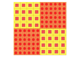
(a)

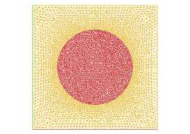
(b)

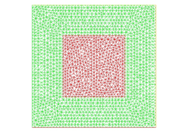
(c)

Figure 1: (a) The macrostructure domain $\Omega$; (b) the unit cell $Q^{1}$; (c) the unit cell $Q^{2}$.

In this example, the inclusion and matrix of $Q^{1}$ and $Q^{2}$ are defined as the identical materia. The detailed material property parameters are listed in Table 1.

Table 1: Material property parameters

Property	Matrix of $\Omega_{1}\cup\Omega_{3}$	Inclusion of $\Omega_{1}\cup\Omega_{3}$
Thermal conductivity$(W/(m\bm{\cdot}K))$	100.0	0.1
Property	Matrix of $\Omega_{2}\cup\Omega_{4}$	Inclusion of $\Omega_{2}\cup\Omega_{4}$
Thermal conductivity$(W/(m\bm{\cdot}K))$	100.0	0.1

The data in problem (1) are given as follows:

$$h(\mathbf{x})=100J/(cm^{3}\bm{\cdot}s),\;\widehat{T}(\mathbf{x})=373.15K\;\;\text{in}\;\;\partial\Omega$$ (38)

Now, we implement the triangular mesh generation to multiscale problem (1), auxiliary cell problems and associated homogenized problem (12). The computational cost of FEM elements and nodes is listed in Table 2.

Table 2: Comparison of computational cost

	Original equation	Cell problem of $Q^{1}$
number of elements	115216	3446
number of nodes	58473	1804
	Cell problem of $Q^{2}$	Homogenized equation
number of elements	3438	53286
number of nodes	1800	26944

Fig. 2 shows the numerical results for solutions $T^{\bm{\varepsilon}}$, $T^{(0)}$, $T^{(1\bm{\varepsilon})}$ and $T^{(2\bm{\varepsilon})}$, respectively.

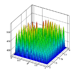
(a)

(b)

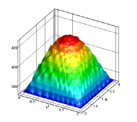
(c)

(d)

Figure 2: The temperature field: (a) $T^{\bm{\varepsilon}}$; (b) $T^{(0)}$; (c) $T^{(1\bm{\varepsilon})}$; (d) $T^{(2\bm{\varepsilon})}$.

After completing numerical computation, the relative $L^{2}$ norm error and $H^{1}$ semi-norm error of temperature field are listed in Table 3.

Table 3: Comparison of relative errors

	Terror0	Terror1	Terror2
Percentage %	6.3920	6.3951	0.0627
	TError0	TError1	TError2
Percentage %	99.6400	99.3812	5.9648

From Table 2, one can see that the computational cost of SOTS method is much less than precise FEM. It means that the SOTS method can greatly save computer memory, which is very important in engineering computation. Fig. 2 demonstrates that only SOTS solution can accurately capture the micro-scale oscillating information due to heterogeneities in composites. From Table 3, we can conclude that only SOTS solution is almost the same as the precise FEM solution. By contrast, homogenized and FOTS solutions are far from enough to provide a high accuracy solution for multiscale problem (1).

5.2 Example 2: different configurations with diverse material

In this example, a 2D composite structures with two basic periodic configurations in four subdomains is considered. The macrostructure $\Omega$ is shown in Fig. 3, where $\Omega=(x,y)=[0,2]\times[0,2]cm^{2}$. Assume that $\Omega=\Omega_{1}\cup\Omega_{2}\cup\Omega_{3}\cup\Omega_{4}$ where $\Omega_{1}=[0,1]\times[0,1]cm^{2}$, $\Omega_{2}=[1,2]\times[0,1]cm^{2}$, $\Omega_{3}=[1,2]\times[1,2]cm^{2}$ and $\Omega_{4}=[0,1]\times[1,2]cm^{2}$. Moreover, $\Omega_{1}$ and $\Omega_{3}$ have the same unit cell $Q^{1}$ with periodic unit cell size $\displaystyle\varepsilon_{1}=\frac{1}{7}$. $\Omega_{2}$ and $\Omega_{4}$ have the same unit cell $Q^{2}$ with periodic unit cell size $\displaystyle\varepsilon_{2}=\frac{1}{5}$.

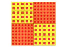
(a)

(b)

(c)

Figure 3: (a) The macrostructure domain $\Omega$; (b) the unit cell $Q^{1}$; (c) the unit cell $Q^{2}$.

In this example, the inclusion of $Q^{1}$ and $Q^{2}$ are defined as different materials. The detailed material property parameters are listed in Table 4.

Table 4: Material property parameters

Property	Matrix of $\Omega_{1}\cup\Omega_{3}$	Inclusion of $\Omega_{1}\cup\Omega_{3}$
Thermal conductivity$(W/(m\bm{\cdot}K))$	100.0	0.5
Property	Matrix of $\Omega_{2}\cup\Omega_{4}$	Inclusion of $\Omega_{2}\cup\Omega_{4}$
Thermal conductivity$(W/(m\bm{\cdot}K))$	100.0	0.1

The data in problem (1) are given as follows:

$$h(\mathbf{x})=200J/(cm^{3}\bm{\cdot}s),\;\widehat{T}(\mathbf{x})=373.15K\;\;\text{in}\;\;\partial\Omega$$ (39)

Now, we implement the triangular mesh generation to multiscale problem (1), auxiliary cell problems and associated homogenized problem (12). The computational cost of FEM elements and nodes is listed in Table 5.

Table 5: Comparison of computational cost

	Original equation	Cell problem of $Q^{1}$
number of elements	169904	3446
number of nodes	85985	1804
	Cell problem of $Q^{2}$	Homogenized equation
number of elements	3438	53286
number of nodes	1800	26944

Fig. 4 shows the numerical results for solutions $T^{\bm{\varepsilon}}$, $T^{(0)}$, $T^{(1\bm{\varepsilon})}$ and $T^{(2\bm{\varepsilon})}$, respectively.

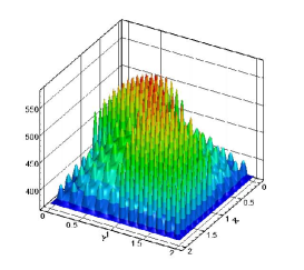
(a)

(b)

(c)

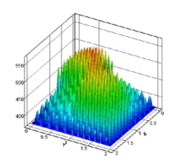
(d)

Figure 4: The temperature field: (a) $T^{\bm{\varepsilon}}$; (b) $T^{(0)}$; (c) $T^{(1\bm{\varepsilon})}$; (d) $T^{(2\bm{\varepsilon})}$.

Afterwards, the relative $L^{2}$ norm error and $H^{1}$ semi-norm error of temperature field are listed in Table 6.

Table 6: Comparison of relative errors

	Terror0	Terror1	Terror2
Percentage %	5.1486	5.1398	1.0740
	TError0	TError1	TError2
Percentage %	99.0826	98.6436	8.8350

From Table 5, one can easily see that the computational cost of SOTS method still is much less than precise FEM. From Fig. 4 , it shows that the SOTS solution is much better than the homogenized and FOTS solutions for temperature field of multiscale problem (1). It is easy to see that only the SOTS solutions can provide enough numerical accuracy for engineering applications from Table 6. The accuracy of homogenized solutions and FOTS solutions is far from enough especially in the $H^{1}$ semi-norm sense.

6 Conclusions

In this paper, we develop a SOTS computational method for heat conduction problems of composite structures with diverse periodic configurations in different subdomains. The new contributions of this paper are the SOTS analysis, the error analysis in the pointwise sense and integral sense for the SOTS solutions, and associated SOTS numerical algorithm. Numerical experiments show that the SOTS numerical method we proposed is effective for multiscale problem (1). Furthermore, numerical results show that only SOTS solutions can accurately capture the microscale oscillating information and provide enough numerical accuracy for engineering applications, which support the theoretical results of this paper.

References

- Matine et al. [2015] A. Matine, N. Boyard, G. Legrain, Y. Jarny, P. Cartraud, Transient heat conduction within periodic heterogeneous media: A space-time homogenization approach, International Journal of Thermal Sciences 92 (2015) 217–229.
- Ma et al. [2016] Q. Ma, J. Cui, Z. Li, Z. Wang, Second-order asymptotic algorithm for heat conduction problems of periodic composite materials in curvilinear coordinates, Journal of Computational and Applied Mathematics 306 (2016) 87–115.
- Yanga et al. [2015] Z. Yanga, J. Cui, Y. Sun, J. Ge, Multiscale computation for transient heat conduction problem with radiation boundary condition in porous materials, Finite Elements in Analysis and Design 102-103 (2015) 7–18.
- Yang et al. [2016] Z. Yang, J. Cui, Z. Wang, Y. Zhang, Multiscale computational method for nonstationary integrated heat transfer problem in periodic porous materials, Numerical Methods for Partial Differential Equations 32 (2016) 510–530.
- Su et al. [2011] F. Su, Z. Xu, Q. Dong, H. Li, A second-order and two-scale computation method for heat conduction equation with rapidly oscillatory coefficients, Finite Elements in Analysis and Design 47 (2011) 276–280.
- Allegretto et al. [2008] W. Allegretto, L. Cao, Y. Lin, Multiscale asymptotic expansion for second order parabolic equations with rapidly oscillating coefficients, Discrete and Continuous Dynamical Systems A 20 (2008) 543–576.
- Wu et al. [2014] Y. T. Wu, Y. F. Nie, Z. H. Yang, Comparison of four multiscale methods for elliptic problems, CMES-Computer Modeling in Engineering Sciences 99 (2014) 297–325.
- Dong et al. [2016] H. Dong, Y. Nie, Z. Yang, Y. Wu, The Numerical Accuracy Analysis of Asymptotic Homogenization Method and Multiscale Finite Element Method for Periodic Composite Materials, CMES-Computer Modeling in Engineering Sciences 111 (2016) 395–419.
- Cui [2001] J. Cui, Multiscale computational method for unified design of structure, components and their materials, in: Proceedings on Computational Mechanics in Science and Engineering, CCCM-2001, Guangzhou, 5-8 December, Peking University Press, 2001, pp. 33–43.
- Cui [1996] J. Cui, The two-scale expression of the solution for the structure with several sub-domains of small periodic configurations, in: WORKSHOP ON SCIENTIFIC COMPUTING 99, Hong Kong, 27-30 June, 1996.
- Oleinik et al. [1992] O. A. Oleinik, A. S. Shamaev, G. A. Yosifian, Mathematical Problems in Elasticity and Homogenization, North-Holland: Amsterdam, 1992.
- Cioranescu and Donato [1999] D. Cioranescu, P. Donato, An Introduction to Homogenization, Oxford University Press, 1999.
- Wang et al. [2015] X. Wang, L. Cao, Y. Wong, Multiscale computation and convergence for coupled thermoelastic system in composite materials, SIAM Multiscale Modeling and Simulation 13 (2015) 661–690.
- Cao [2006] L. Cao, Multiscale asymptotic expansion and finite element methods for the mixed boundary value problems of second order elliptic equation in perforated domains, Numerische Mathematik 103 (2006) 11–45.
- Dong and Cao [2009] Q. Dong, L. Cao, Multiscale asymptotic expansions methods and numerical algorithms for the wave equations of second order with rapidly oscillating coefficients, Applied Numerical Mathematics 59 (2009) 3008–3032.
- Lin and Zhu [1994] Q. Lin, Q. Zhu, The Preprocessing snd Preprocessing for the Finite Element Method, Shanghai Scientific Technical Publishers, 1994.