Inverse elastic surface scattering with far-field data

Abstract.

A rigorous mathematical model and an efficient computational method are proposed to solving the inverse elastic surface scattering problem which arises from the near-field imaging of periodic structures. We demonstrate how an enhanced resolution can be achieved by using more easily measurable far-field data. The surface is assumed to be a small and smooth perturbation of an elastically rigid plane. By placing a rectangular slab of a homogeneous and isotropic elastic medium with larger mass density above the surface, more propagating wave modes can be utilized from the far-field data which contributes to the reconstruction resolution. Requiring only a single illumination, the method begins with the far-to-near (FtN) field data conversion and utilizes the transformed field expansion to derive an analytic solution for the direct problem, which leads to an explicit inversion formula for the inverse problem. Moreover, a nonlinear correction scheme is developed to improve the accuracy of the reconstruction. Results show that the proposed method is capable of stably reconstructing surfaces with resolution controlled by the slab’s density.

1. Introduction

Scattering problems have been studied extensively in the past decades [15]. They have many significant applications in many science and engineering areas such as radar and sonar, medical imaging, and remote sensing. Especially, the elastic wave scattering problems have practical applications in geophysics, seismology, and nondestructive testing [1, 2, 3, 11]. There are two kinds of problems: the direct scattering problems are to determine the wave field from the differential equations governing the wave motion; the inverse scattering problems are to determine the unknown medium, such as the geometry or material, from the measurement of the wave field. In this paper we focus on the inverse elastic scattering problem in periodic structures. The direct elastic scattering problem has been studied by many researchers [5, 4, 17, 19]. The uniqueness result of the inverse problem can be found in [13]. The numerical study can be found in [18] and [20] for the inverse problem by using an optimization method and the factorization method, respectively.

It is known that there is a resolution limit to the sharpness of the details which can be observed from conventional far-field optical microscopy, one half the wavelength, referred to as the Rayleigh criterion or the diffraction limit [16]. The loss of resolution is mainly due to the ignorance of the evanescent wave components. Near-field optical imaging is an effective approach to obtain images with subwavelength resolution. The inverse scattering problems via the near-field imaging for acoustic and electromagnetic waves have been undergoing extensive studies for impenetrable infinite rough surfaces [7], penetrable infinite rough surfaces [9], two- and three-dimensional diffraction gratings [6, 8, 14, 21], bounded obstacles [24], and interior cavities [23]. The two- and three-dimensional inverse elastic surface scattering problems have been investigated by using near-field data in [25, 26, 27]. However, there exits some difficulties of near-field optical imaging in practice, for example, it requires a sophisticated control of the probe when scanning samples to measure the near-field data. Recently, a rigorous mathematical model and an efficient numerical method are proposed in [10] to over the aforementioned obstacle in near-field imaging. The novel idea is to put a rectangular slab of larger index of refraction above the surfaces and allow more propagating wave modes to be able to propagate to the far-field regime. This work is devoted to the inverse elastic surface scattering problem with far-field data. We point out that this is a nontrivial extension of the method from solving the inverse acoustic surface scattering problem to solving the inverse elastic surface scattering problem, because the latter involves the more complicated elastic wave equation due to the coexistence of compressional and shear waves propagating at different speeds.

In this paper, we develop a rigorous mathematical model and an efficient numerical method for the inverse elastic surface scattering with far-field data. The scattering surface is assumed to be a small and smooth perturbation of an elastically rigid plane. A rectangular slab of homogeneous and isotropic elastic medium is placed above the scattering surface. The slab has a larger mass density than that of the free space, and has a wavelength comparable thickness. The measurement can be took on the top face of the slab, which is in the far-field regime. The method makes use of the Helmholtz decomposition to consider two coupled Helmholtz equations instead of the elastic wave equation. It consists of two steps. The first step is to do the far-to-near (FtN) field data conversion, which requires to solve a Cauchy problem of the Helmholtz equation in the slab. Using the Fourier analysis, we compute the analytic solution and find a formula connecting the wave fields on the top and bottom faces of the slab: a larger mass density of the slab allows more propagating wave modes to be converted stably from the far-field regime to the near-field regime. The second step is to solve an inverse surface scattering problem in the near-field zone by using the data obtained from the first step. Combining the Fourier analysis, we use the transformed field expansions to find an analytic solution for the direct problem. We refer to [12, 28, 29, 30, 22] for the transformed field expansion and related boundary perturbation methods for solving direct surface scattering problems. Using the closed form of the analytic solution, we deduce expressions for the leading and linear terms of the power series solution. Dropping all higher order terms, we linearize the inverse problem and obtain explicit reconstruction formulas for the surface function. Moreover, a nonlinear correction scheme is also developed to improve the reconstruction. The method requires only a single illumination and is implemented efficiently by the fast Fourier transform (FFT). Numerical examples show it is effective and robust to reconstruct the scattering surfaces with subwavelength resolution.

The remaining part of the paper is organized as follows. The mathematical model problem is formulated in Section 2. Sections 3 and 4 introduce the Helmholtz decomposition and the transparent boundary condition, respectively. In Section 5, we show how to convert the measured elastic wave data into the scattering data of the scalar potentials introduced from the Helmholtz decomposition. In Section 6, a reduced problem is modeled in the slab and the analytic solution is obtained to accomplish the FtN field data conversion. In Section 7, the transformed field expansion and corresponding recursive boundary value problems are presented. We give the reconstruction formulas for the inverse problem in Section 8. Numerical experiments are presented in Section 9 to demonstrate the effectiveness of the proposed method. Finally, we conclude some general remarks and directions for future research in Section 10.

2. Model problem

Let us first introduce the problem geometry, which is shown in Figure 1. Consider an elastically rigid surface $\Gamma_{f}=\{\boldsymbol{x}=(x,y)\in\mathbb{R}^{2}:y=f(x),\,0<x<\Lambda\}$, where $f$ is a periodic Lipschitz continuous function with period $\Lambda$. The scattering surface function $f$ is assumed to have the form

$$f(x)=\varepsilon g(x),$$ (2.1)

where $\varepsilon>0$ is a sufficiently small constant and is called the surface deformation parameter, $g$ is the surface profile function which is also periodic with the period $\Lambda$. Hence the surface $\Gamma_{f}$ is a small perturbation of the planar surface $\Gamma_{0}=\{\boldsymbol{x}\in\mathbb{R}^{2}:y=0,\,0<x<\Lambda\}.$ Let a rectangular slab of homogeneous and isotropic elastic medium be placed above the scattering surface. The bottom face of the slab is $\Gamma_{b}=\{\boldsymbol{x}\in\mathbb{R}^{2}:y=b,\,0<x<\Lambda\},$ where $b>\max_{x\in(0,\Lambda)}f(x)$ is a constant and stands for the separation distance between the scattering surface and the slab. The top face of the slab is $\Gamma_{a}=\{\boldsymbol{x}\in\mathbb{R}^{2}:y=a,\,0<x<\Lambda\},$ where $a>b$ is a positive constant and stands for the measurement distance. Denote by $\Omega$ the bounded domain between $\Gamma_{f}$ and $\Gamma_{b}$, i.e., $\Omega=\{\boldsymbol{x}\in\mathbb{R}^{2}:f<y<b,\,0<x<\Lambda\}.$ Let $R$ be the domain of the slab, i.e., $R=\{\boldsymbol{x}\in\mathbb{R}^{2}:b<y<a,\,0<x<\Lambda\}.$ Finally, denote by $U$ the open domain above $\Gamma_{a}$, i.e., $U=\{\boldsymbol{x}\in\mathbb{R}^{2}:y>a,\,0<x<\Lambda\}.$

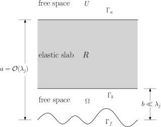
Figure 1. The problem geometry.

In this paper, we assume for simplicity that the Lamé parameters $\mu,\lambda$ are constants satisfying $\mu>0,\lambda+\mu>0$; the mass density $\rho$ is a piecewise constant, i.e.,

$$\rho(\boldsymbol{x})=\begin{cases}\rho_{0},\quad\boldsymbol{x}\in\Omega\cup U,\\ \rho_{1},\quad\boldsymbol{x}\in R,\end{cases}$$

where $\rho_{0}$ and $\rho_{1}$ are the density of the free space and the elastic slab, respectively, and they satisfy $\rho_{1}>\rho_{0}>0$. Define

$$\kappa_{1}=\omega\left(\frac{\rho_{0}}{\lambda+2\mu}\right)^{1/2},\quad\kappa_{2}=\omega\left(\frac{\rho_{0}}{\mu}\right)^{1/2},$$

which are known as the compressional wavenumber and the shear wavenumber in the free space, respectively. We comment that the method also works for the case where $\mu,\lambda$ take different values in the free space and the elastic slab. Let $\lambda_{j}=2\pi/\kappa_{j},j=1,2$ be the corresponding wavelength of the compressional and shear waves.

Let $\boldsymbol{u}^{\rm inc}$ be a time-harmonic plane wave which is incident on the slab from above. The incident plane wave can be taken as either the compressional wave $\boldsymbol{u}^{\rm inc}(\boldsymbol{x})=\boldsymbol{d}e^{{\rm i}\kappa_{1}\boldsymbol{x}\cdot\boldsymbol{d}}$ or the shear wave $\boldsymbol{u}^{\rm inc}=\boldsymbol{d}^{\perp}e^{{\rm i}\kappa_{2}\boldsymbol{x}\cdot\boldsymbol{d}}$, where $\boldsymbol{d}=(\sin\theta,-\cos\theta)^{\top}$ is the unit incident direction vector, $\theta\in(-\pi/2,\pi/2)$ is the incident angle, and $\boldsymbol{d}^{\perp}=(\cos\theta,\sin\theta)^{\top}$ is an orthonormal vector to $\boldsymbol{d}$. In this work, we use the compressional incident plane wave as an example to present the results, which are similar and can be obtained with obvious modifications for the shear incident plane wave. Practically, the simplest configuration is the normal incidence for experiments, i.e., $\theta=0$. Hence we focus on the normal incidence since our method requires only a single illumination. Under the normal incidence, the incident field reduces to

$$\boldsymbol{u}^{\rm inc}(\boldsymbol{x})=(0,-1)^{\top}e^{-{\rm i}\kappa_{1}y}.$$ (2.2)

It can be verified that the incident field $\boldsymbol{u}^{\rm inc}$ satisfies the elastic wave equation:

$$\mu\Delta\boldsymbol{u}^{\rm inc}+(\lambda+\mu)\nabla\nabla\cdot\boldsymbol{u}^{\rm inc}+\omega^{2}\rho_{0}\boldsymbol{u}^{\rm inc}=0\quad\text{in}~{}U.$$ (2.3)

A transmission problem can be formulated due to the interaction between the elastic wave and the interfaces $\Gamma_{a}$ and $\Gamma_{b}$. Let $\boldsymbol{u},\boldsymbol{v},\boldsymbol{w}$ be the displacements of the total field in the domains $U,R,\Omega$, respectively. They satisfy the elastic wave equations:

$$\mu\Delta\boldsymbol{u}+(\lambda+\mu)\nabla\nabla\cdot\boldsymbol{u}+\omega^{2}\rho_{0}\boldsymbol{u}=0 \quad\text{in}~{}U,$$ (2.4a)

$$\mu\Delta\boldsymbol{v}+(\lambda+\mu)\nabla\nabla\cdot\boldsymbol{v}+\omega^{2}\rho_{1}\boldsymbol{v}=0 \quad\text{in}~{}R,$$ (2.4b)

$$\mu\Delta\boldsymbol{w}+(\lambda+\mu)\nabla\nabla\cdot\boldsymbol{w}+\omega^{2}\rho_{0}\boldsymbol{w}=0 \quad\text{in}~{}\Omega.$$ (2.4c)

In addition, the total fields are connected by the continuity conditions:

$$\boldsymbol{u}=\boldsymbol{v}, \quad\mu\partial_{y}\boldsymbol{u}+(\lambda+\mu)(0,1)^{\top}\nabla\cdot\boldsymbol{u}=\mu\partial_{y}\boldsymbol{v}+(\lambda+\mu)(0,1)^{\top}\nabla\cdot\boldsymbol{v}\quad\text{on}~{}\Gamma_{a},$$ (2.5a)

$$\boldsymbol{v}=\boldsymbol{w}, \quad\mu\partial_{y}\boldsymbol{v}+(\lambda+\mu)(0,1)^{\top}\nabla\cdot\boldsymbol{v}=\mu\partial_{y}\boldsymbol{w}+(\lambda+\mu)(0,1)^{\top}\nabla\cdot\boldsymbol{w}\quad\text{on}~{}\Gamma_{b}.$$ (2.5b)

Since $\Gamma_{f}$ is elastically rigid, we have the homogeneous Dirichlet boundary condition:

$$\boldsymbol{w}=0\quad\text{on}~{}\Gamma_{f}.$$ (2.6)

In the open domain $U$, the total field $\boldsymbol{u}$ consists of the incident field $\boldsymbol{u}^{\rm inc}$ and the diffracted field $\boldsymbol{u}^{\rm d}$:

$$\boldsymbol{u}=\boldsymbol{u}^{\rm inc}+\boldsymbol{u}^{\rm d},$$ (2.7)

where $\boldsymbol{u}^{\rm d}$ is required to satisfy the bounded outgoing wave condition.

Throughout, we assume that the measurement distance $a=\mathcal{O}(\lambda_{j})$ and the separation distance $b\ll\lambda_{j}$, i.e., $a$ is comparable with the wavelength and $\Gamma_{a}$ is put in the far-field region; $b$ is much smaller than the wavelength and $\Gamma_{b}$ is put in the near-field region. Now we are ready to formulate the inverse problem: Given the incident field $\boldsymbol{u}^{\rm inc}$, the inverse problem is to determine the scattering surface $f$ from the far-field measurement of the total field $\boldsymbol{u}$ on $\Gamma_{a}$.

3. The Helmholtz decomposition

In this section, we introduce the Helmholtz decomposition for the total fields by using scalar potential functions, and deduce the continuity conditions for these scalar fields. Let $\boldsymbol{u}=(u_{1},u_{2})^{\top}$ and $u$ be a vector and a scalar function, respectively. Introduce the scalar and vector curl operators:

$${\rm curl}\boldsymbol{u}=\partial_{x}u_{2}-\partial_{y}u_{1},\quad{\bf curl}u=(\partial_{y}u,-\partial_{x}u)^{\top}.$$

For any solution $\boldsymbol{u}=(u_{1},u_{2})^{\top}$ of (2.4a), the Helmholtz decomposition reads

$$\boldsymbol{u}=\nabla\phi_{1}+{\bf curl}\phi_{2},$$ (3.1)

where $\phi_{j},j=1,2$ are two scalar potential functions. Explicitly, we have

$$u_{1}=\partial_{x}\phi_{1}+\partial_{y}\phi_{2},\quad u_{2}=\partial_{y}\phi_{1}-\partial_{x}\phi_{2}.$$ (3.2)

Substituting (3.1) into (2.4a) yields

$$\nabla\left((\lambda+2\mu)\Delta\phi_{1}+\omega^{2}\rho_{0}\phi_{1}\right)+{\bf curl}\left(\mu\Delta\phi_{2}+\omega^{2}\rho_{0}\phi_{2}\right)=0,$$

which is fulfilled if $\phi_{j}$ satisfies

$$\Delta\phi_{j}+\kappa^{2}_{j}\phi_{j}=0\quad\text{in}~{}U.$$ (3.3)

Combining (3.3) and (3.1), we obtain

$$\phi_{1}=-\frac{1}{\kappa_{1}^{2}}\nabla\cdot\boldsymbol{u},\quad\phi_{2}=\frac{1}{\kappa_{2}^{2}}{\rm curl}\boldsymbol{u},$$

which give

$$\partial_{x}u_{1}+\partial_{y}u_{2}=-\kappa_{1}^{2}\phi_{1},\quad\partial_{x}u_{2}-\partial_{y}u_{1}=\kappa_{2}^{2}\phi_{2}.$$ (3.4)

For any solution $\boldsymbol{v}=(v_{1},v_{2})^{\top}$ of (2.4b), we introduce the Helmholtz decomposition by using scalar functions $\psi_{j}$:

$$\boldsymbol{v}=\nabla\psi_{1}+{\bf curl}\psi_{2},$$ (3.5)

which gives explicitly that

$$v_{1}=\partial_{x}\psi_{1}+\partial_{y}\psi_{2},\quad v_{2}=\partial_{y}\psi_{1}-\partial_{x}\psi_{2}.$$ (3.6)

Plugging (3.5) into (2.4b), we may have

$$\Delta\psi_{j}+\eta_{j}^{2}\psi_{j}=0\quad\text{in}~{}R,$$ (3.7)

where $\eta_{1}$ and $\eta_{2}$ are the compressional and shear wavenumbers in the elastic slab, respectively, and are given by

$$\eta_{1}=\omega\left(\frac{\rho_{1}}{\lambda+2\mu}\right)^{1/2},\quad\eta_{2}=\omega\left(\frac{\rho_{1}}{\mu}\right)^{1/2}.$$ (3.8)

Combing (3.7) and (3.5), we get

$$\psi_{1}=-\frac{1}{\eta_{1}^{2}}\nabla\cdot\boldsymbol{v},\quad\psi_{2}=\frac{1}{\eta_{2}^{2}}{\rm curl}\boldsymbol{v},$$

which give

$$\partial_{x}v_{1}+\partial_{y}v_{2}=-\eta_{1}^{2}\psi_{1},\quad\partial_{x}v_{2}-\partial_{y}v_{1}=\eta_{2}^{2}\psi_{2}.$$ (3.9)

Since $\Gamma_{a}$ is a horizontal line, it is easy to verify from the continuity condition (2.5a) that

$$u_{j}=v_{j},\quad\partial_{y}u_{j}=\partial_{y}v_{j}.$$ (3.10)

Using (3.4), (3.9)–(3.10), we deduce the first continuity condition for the scalar potentials on $\Gamma_{a}$:

$$\kappa_{j}^{2}\phi_{j}=\eta_{j}^{2}\psi_{j}.$$ (3.11)

It follows from (3.2), (3.6), and (3.10) that we deduce the second continuity condition for the scalar potentials on $\Gamma_{a}$:

$$\partial_{y}\phi_{1}-\partial_{x}\phi_{2}=\partial_{y}\psi_{1}-\partial_{x}\psi_{2},\quad\partial_{y}\phi_{2}+\partial_{x}\phi_{1}=\partial_{y}\psi_{2}+\partial_{x}\psi_{1}.$$ (3.12)

Similarly, for any solution $\boldsymbol{w}=(w_{1},w_{2})^{\top}$ of (2.4c), the Helmholtz decomposition is

$$\boldsymbol{w}=\nabla\varphi_{1}+{\bf curl}\varphi_{2}.$$ (3.13)

Substituting (3.13) into (2.4c), we may get

$$\Delta\varphi_{j}+\kappa_{j}^{2}\varphi_{j}=0\quad\text{in}~{}\Omega.$$

Noting (2.5b), we may repeat the same steps and obtain the continuity conditions on $\Gamma_{b}$:

$$\eta_{j}^{2}\psi_{j}=\kappa_{j}^{2}\varphi_{j}$$ (3.14)

and

$$\partial_{y}\psi_{1}-\partial_{x}\psi_{2}=\partial_{y}\varphi_{1}-\partial_{x}\varphi_{2},\quad\partial_{y}\psi_{2}+\partial_{x}\psi_{1}=\partial_{y}\varphi_{2}+\partial_{x}\varphi_{1}.$$ (3.15)

Finally, it follows from the boundary condition (2.6) and the Helmholtz decomposition (3.13) that

$$\partial_{x}\varphi_{1}+\partial_{y}\varphi_{2}=0,\quad\partial_{y}\varphi_{1}-\partial_{x}\varphi_{2}=0\quad\text{on}~{}\Gamma_{f}.$$ (3.16)

4. Transparent boundary condition

It follows from (2.3), (2.4a), and (2.7) that the diffracted field $\boldsymbol{u}^{\rm d}$ also satisfies the elastic wave equation:

$$\mu\Delta\boldsymbol{u}^{\rm d}+(\lambda+\mu)\nabla\nabla\cdot\boldsymbol{u}^{\rm d}+\omega^{2}\rho_{0}\boldsymbol{u}^{\rm d}=0\quad\text{in}~{}U.$$ (4.1)

Introduce the Helmholtz decomposition for the diffracted field $\boldsymbol{u}^{\rm d}$:

$$\boldsymbol{u}^{\rm d}=\nabla\phi^{\rm d}_{1}+{\bf curl}\phi^{\rm d}_{2},$$ (4.2)

Substituting (4.2) into (4.1) may yield

$$\Delta\phi^{\rm d}_{j}+\kappa^{2}_{j}\phi^{\rm d}_{j}=0\quad\text{in}~{}U.$$ (4.3)

It follows from the uniqueness of the solution for the direct problem that $\phi^{\rm d}_{j}$ is a periodic function with period $\Lambda$ and admits the Fourier series expansion:

$$\phi^{\rm d}_{j}(x,y)=\sum_{n\in\mathbb{Z}}\phi^{\rm d}_{jn}(y)e^{{\rm i}\alpha_{n}x},$$ (4.4)

where $\alpha_{n}=2n\pi/\Lambda$. Plugging (4.4) into (4.3) yields

$$\partial^{2}_{yy}\phi^{\rm d}_{jn}(y)+\beta_{jn}^{2}\phi^{\rm d}_{jn}(y)=0,\quad y>a,$$ (4.5)

where

$$\beta_{jn}=\begin{cases}(\kappa_{j}^{2}-\alpha_{n}^{2})^{1/2},&\quad|\alpha_{n}|<\kappa_{j},\\ {\rm i}(\alpha_{n}^{2}-\kappa_{j}^{2})^{1/2},&\quad|\alpha_{n}|>\kappa_{j}.\end{cases}$$

Here we assume that $\beta_{jn}\neq 0$ to exclude possible resonance.

Using the bounded outgoing wave condition, we may solve (4.5) analytically and obtain the solution of (4.3) explicitly:

$$\phi^{\rm d}_{j}(x,y)=\sum_{n\in\mathbb{Z}}\phi^{\rm d}_{jn}(a)e^{{\rm i}(\alpha_{n}x+\beta_{jn}(y-a))},$$ (4.6)

which is called the Rayleigh expansion for the scalar potential function $\phi^{\rm d}_{j}$. Taking the normal derivative of (4.6) on $\Gamma_{a}$ gives

$$\partial_{y}\phi^{\rm d}_{j}(x,a)=\sum_{n\in\mathbb{Z}}{\rm i}\beta_{jn}\phi^{\rm d}_{jn}(a)e^{{\rm i}\alpha_{n}x}.$$ (4.7)

For a given periodic function $u(x)$ with period $\Lambda$, it has the Fourier series expansion:

$$u(x)=\sum_{n\in\mathbb{Z}}u_{n}e^{{\rm i}\alpha_{n}x},\quad u_{n}=\frac{1}{\Lambda}\int_{0}^{\Lambda}u(x)e^{-{\rm i}\alpha_{n}x}{\rm d}x.$$

We define the boundary operator:

$$(\mathscr{T}_{j}u)(x)=\sum_{n\in\mathbb{Z}}{\rm i}\beta_{jn}u_{n}e^{{\rm i}\alpha_{n}x}.$$

It is easy to verify from (4.7) that

$$\partial_{y}\phi^{\rm d}_{j}=\mathscr{T}_{j}\phi^{\rm d}_{j}\quad\text{on}~{}\Gamma_{a}.$$ (4.8)

Recalling the incident field (2.2), we may also consider the Helmholtz decomposition for the incident field:

$$\boldsymbol{u}^{\rm inc}=\nabla\phi_{1}^{\rm inc}+{\bf curl}\phi_{2}^{\rm inc},$$ (4.9)

which gives

$$\phi_{1}^{\rm inc}=-\frac{1}{\kappa_{1}^{2}}\nabla\cdot\boldsymbol{u}^{\rm inc}=-\frac{\rm i}{\kappa_{1}}e^{-{\rm i}\kappa_{1}y},\quad\phi_{2}^{\rm inc}=\frac{1}{\kappa_{2}^{2}}{\rm curl}\boldsymbol{u}^{\rm inc}=0.$$

A simple calculation yields

$$\partial_{y}\phi_{1}^{\rm inc}=-e^{-{\rm i}\kappa_{1}a},\quad\mathscr{T}_{1}\phi_{1}^{\rm inc}=e^{-{\rm i}\kappa_{1}a},$$

which gives

$$\partial_{y}\phi_{1}^{\rm inc}=\mathscr{T}_{1}\phi_{1}^{\rm inc}+g_{1},\quad\partial_{y}\phi_{2}^{\rm inc}=\mathscr{T}_{2}\phi_{2}^{\rm inc}+g_{2}.$$ (4.10)

Here $g_{1}=-2e^{-{\rm i}\kappa_{1}a}$ and $g_{2}=0$.

Letting $\phi_{j}=\phi_{j}^{\rm inc}+\phi^{\rm d}_{j}$ and recalling $\boldsymbol{u}=\boldsymbol{u}^{\rm inc}+\boldsymbol{u}^{\rm d}$, we get (3.1) by adding (4.9) and (4.2). Moreover, we obtain the transparent boundary condition for the total scalar potentials by combing (4.8) and (4.10):

$$\partial_{y}\phi_{j}=\mathscr{T}_{j}\phi_{j}+g_{j}\quad\text{on}~{}\Gamma_{a}.$$ (4.11)

It follows from (3.11)–(3.12) that

$$\partial_{y}\phi_{1} =\partial_{y}\psi_{1}-\partial_{x}\psi_{2}+\partial_{x}\phi_{2}=\partial_{y}\psi_{1}-\partial_{x}\psi_{2}+\left(\frac{\eta_{2}^{2}}{\kappa_{2}^{2}}\right)\partial_{x}\psi_{2}$$

$$=\partial_{y}\psi_{1}+\left(\frac{\eta_{2}^{2}-\kappa_{2}^{2}}{\kappa_{2}^{2}}\right)\partial_{x}\psi_{2},$$

$$\partial_{y}\phi_{2} =\partial_{y}\psi_{2}+\partial_{x}\psi_{1}-\partial_{x}\phi_{1}=\partial_{y}\psi_{2}+\partial_{x}\psi_{1}-\left(\frac{\eta_{1}^{2}}{\kappa_{1}^{2}}\right)\partial_{x}\psi_{1}$$

$$=\partial_{y}\psi_{2}-\left(\frac{\eta_{1}^{2}-\kappa_{1}^{2}}{\kappa_{1}^{2}}\right)\partial_{x}\psi_{1}.$$ (4.12)

Combining (4.11)–(4) and (3.11) yields the boundary condition for $\psi_{j}$ on $\Gamma_{a}$:

$$\partial_{y}\psi_{1}+\left(\frac{\eta_{2}^{2}-\kappa_{2}^{2}}{\kappa_{2}^{2}}\right)\partial_{x}\psi_{2} =\left(\frac{\eta_{1}^{2}}{\kappa_{1}^{2}}\right)\mathscr{T}_{1}\psi_{1}+g_{1},$$

$$\partial_{y}\psi_{2}-\left(\frac{\eta_{1}^{2}-\kappa_{1}^{2}}{\kappa_{1}^{2}}\right)\partial_{x}\psi_{1} =\left(\frac{\eta_{2}^{2}}{\kappa_{2}^{2}}\right)\mathscr{T}_{2}\psi_{2}+g_{2}.$$ (4.13)

Let $\boldsymbol{u}$ be a periodic function of $x$ with period $\Lambda$. It admits the Fourier series expansion:

$$\boldsymbol{u}(x)=\sum_{n\in\mathbb{Z}}\boldsymbol{u}_{n}e^{{\rm i}\alpha_{n}x},\quad\boldsymbol{u}_{n}=\frac{1}{\Lambda}\int_{0}^{\Lambda}\boldsymbol{u}(x)e^{-{\rm i}\alpha_{n}x}{\rm d}x.$$

Define the boundary operator on $\Gamma_{a}$:

$$(\mathscr{T}\boldsymbol{u})(x)=\sum_{n\in\mathbb{Z}}{\rm i}\begin{bmatrix}\frac{\omega^{2}\beta_{1n}}{\alpha_{n}^{2}+\beta_{1n}\beta_{2n}}&\mu\alpha_{n}-\frac{\omega^{2}\alpha_{n}^{2}}{\alpha_{n}^{2}+\beta_{1n}\beta_{2n}}\\[5.0pt] \frac{\omega^{2}\alpha_{n}^{2}}{\alpha_{n}^{2}+\beta_{1n}\beta_{2n}}-\mu\alpha_{n}&\frac{\omega^{2}\beta_{2n}}{\alpha_{n}^{2}+\beta_{1n}\beta_{2n}}\end{bmatrix}\boldsymbol{u}_{n}e^{{\rm i}\alpha_{n}x}.$$

It is shown in [25] that $\alpha_{n}^{2}+\beta_{1n}\beta_{2n}\neq 0$ for $n\in\mathbb{Z}$ and the diffracted field $\boldsymbol{u}^{\rm d}$ satisfies the transparent boundary condition:

$$\mu\partial_{y}\boldsymbol{u}^{\rm d}+(\lambda+\mu)(0,1)^{\top}\nabla\cdot\boldsymbol{u}^{\rm d}=\mathscr{T}\boldsymbol{u}^{\rm d}\quad\text{on}~{}\Gamma_{a}.$$

A simple calculation yields that

$$\mu\partial_{y}\boldsymbol{u}^{\rm inc}+(\lambda+\mu)(0,1)^{\top}\nabla\cdot\boldsymbol{u}^{\rm inc}={\rm i}\kappa_{1}(\lambda+2\mu)(0,1)^{\top}e^{-{\rm i}\kappa_{1}a}$$

and

$$\mathscr{T}\boldsymbol{u}^{\rm inc}=-{\rm i}\kappa_{1}(\lambda+2\mu)(0,1)^{\top}e^{-{\rm i}\kappa_{1}a}.$$

Hence we obtain the boundary condition for the total displacement field $\boldsymbol{u}$:

$$\mu\partial_{y}\boldsymbol{u}+(\lambda+\mu)(0,1)^{\top}\nabla\cdot\boldsymbol{u}=\mathscr{T}\boldsymbol{u}+\boldsymbol{h}\quad\text{on}~{}\Gamma_{a},$$

where $\boldsymbol{h}=2{\rm i}\kappa_{1}(\lambda+2\mu)(0,1)^{\top}e^{-{\rm i}\kappa_{1}a}$. Noting the continuity condition (2.5a), we have

$$\mu\partial_{y}\boldsymbol{v}+(\lambda+\mu)(0,1)^{\top}\nabla\cdot\boldsymbol{v}=\mathscr{T}\boldsymbol{v}+\boldsymbol{h}\quad\text{on}~{}\Gamma_{a}.$$

5. Scattering data

We assume that the total field $\boldsymbol{u}$ is measured on $\Gamma_{a}$, i.e., $\boldsymbol{u}(x,a)=(u_{1}(x,a),u_{2}(x,a))^{\top}$ is available for $x\in(0,\Lambda)$. In this section, we show how to convert $\boldsymbol{u}(x,a)$ into the scattering data of the scalar potentials $\phi_{j}(x,a)$.

Evaluating (3.2) on $\Gamma_{a}$, we have

$$\partial_{x}\phi_{1}(x,a)+\partial_{y}\phi_{2}(x,a)=u_{1}(x,a),\quad\partial_{y}\phi_{1}(x,a)-\partial_{x}\phi_{2}(x,a)=u_{2}(x,a).$$ (5.1)

Let $\phi_{j}(x,a)$ admit the Fourier series expansion

$$\phi_{j}(x,a)=\sum_{n\in\mathbb{Z}}\phi_{jn}e^{{\rm i}\alpha_{n}x}.$$ (5.2)

It suffices to find all the Fourier coefficients of $\phi_{jn}$ in order to determine $\phi_{j}(x,a)$.

Taking the derivative of (5.2) with respect to $x$ yields

$$\partial_{x}\phi_{j}(x,a)=\sum_{n\in\mathbb{Z}}{\rm i}\alpha_{n}\phi_{jn}e^{{\rm i}\alpha_{n}x}.$$ (5.3)

It follows from the transparent boundary condition (4.11) that

$$\partial_{y}\phi_{j}(x,a)=\sum_{n\in\mathbb{Z}}{\rm i}\beta_{jn}\phi_{jn}e^{{\rm i}\alpha_{n}x}+g_{j}.$$ (5.4)

Substituting (5.3) and (5.4) into (5.1), we obtain a linear system of equations for the Fourier coefficients $\phi_{jn}$:

$${\rm i}\begin{bmatrix}\alpha_{n}&\beta_{2n}\\ \beta_{1n}&-\alpha_{n}\end{bmatrix}\begin{bmatrix}\phi_{1n}\\ \phi_{2n}\end{bmatrix}=\begin{bmatrix}p_{1n}\\ p_{2n}\end{bmatrix},$$ (5.5)

where $p_{1n}=u_{1n}-g_{2n}$, $p_{2n}=u_{2n}-g_{1n}$ and $u_{jn}$ are the Fourier coefficients of $u_{j}$, i.e.,

$$u_{jn}=\frac{1}{\Lambda}\int_{0}^{\Lambda}u_{j}(x,a)e^{-{\rm i}\alpha_{n}x}{\rm d}x$$

and

$$g_{1n}=\begin{cases}-2e^{-{\rm i}\kappa_{1}a}&\quad\text{for}~{}n=0,\\ 0&\quad\text{for}~{}n\neq 0,\end{cases}\quad g_{2n}=0~{}\text{for}~{}n\in\mathbb{Z}.$$

Using Cramer’s rule, we obtain the unique solution of (5.5):

$$\phi_{1n}=-{\rm i}\left(\frac{\alpha_{n}p_{1n}+\beta_{2n}p_{2n}}{\alpha_{n}^{2}+\beta_{1n}\beta_{2n}}\right),\quad\phi_{2n}={\rm i}\left(\frac{\alpha_{n}p_{2n}-\beta_{1n}p_{1n}}{\alpha_{n}^{2}+\beta_{1n}\beta_{2n}}\right).$$ (5.6)

Hence, we may assume that $\phi_{j}(x,a),j=1,2$ are measured data. From now on, we shall only work on the potential functions.

6. Reduced problem

Recall the continuity condition (3.11) and the boundary condition (4). Given the data $\phi_{j}$ on $\Gamma_{a}$, we consider the Cauchy problem for $\psi_{j}$:

$$\Delta\psi_{j}+\eta_{j}^{2}\psi_{j}=0 \quad\text{in}~{}R,$$ (6.1a)

$$\psi_{j}=\left(\frac{\kappa_{j}^{2}}{\eta_{j}^{2}}\right)\phi_{j} \quad\text{on}~{}\Gamma_{a},$$ (6.1b)

$$\partial_{y}\psi_{1}+\left(\frac{\eta_{2}^{2}-\kappa_{2}^{2}}{\kappa_{2}^{2}}\right)\partial_{x}\psi_{2}=\left(\frac{\eta_{1}^{2}}{\kappa_{1}^{2}}\right)\mathscr{T}_{1}\psi_{1}+g_{1} \quad\text{on}~{}\Gamma_{a},$$ (6.1c)

$$\partial_{y}\psi_{2}-\left(\frac{\eta_{1}^{2}-\kappa_{1}^{2}}{\kappa_{1}^{2}}\right)\partial_{x}\psi_{1}=\left(\frac{\eta_{2}^{2}}{\kappa_{2}^{2}}\right)\mathscr{T}_{2}\psi_{2}+g_{2} \quad\text{on}~{}\Gamma_{a}.$$ (6.1d)

Since $\psi_{j}$ is a periodic function of $x$, it has the Fourier series expansion

$$\psi_{j}(x,y)=\sum_{n\in\mathbb{Z}}\psi_{jn}(y)e^{{\rm i}\alpha_{n}x}.$$ (6.2)

Substituting (6.2) into (6.1), we obtain a final value problem for the second order equation in the frequency domain:

$$\partial^{2}_{yy}\psi_{jn}(y)+\gamma_{jn}^{2}\psi_{jn}(y)=0, \quad b<y<a,$$ (6.3a)

$$\psi_{jn}(a)=\left(\frac{\kappa_{j}^{2}}{\eta_{j}^{2}}\right)\phi_{jn}, \quad y=a,$$ (6.3b)

$$\partial_{y}\psi_{1n}(a)+{\rm i}\alpha_{n}\left(\frac{\eta_{2}^{2}-\kappa_{2}^{2}}{\kappa_{2}^{2}}\right)\psi_{2n}(a)={\rm i}\beta_{1n}\left(\frac{\eta_{1}^{2}}{\kappa_{1}^{2}}\right)\psi_{1n}(a)+g_{1n}, \quad y=a,$$ (6.3c)

$$\partial_{y}\psi_{2n}(a)-{\rm i}\alpha_{n}\left(\frac{\eta_{1}^{2}-\kappa_{1}^{2}}{\kappa_{1}^{2}}\right)\psi_{1n}(a)={\rm i}\beta_{2n}\left(\frac{\eta_{2}^{2}}{\kappa_{2}^{2}}\right)\psi_{2n}(a)+g_{2n}, \quad y=a,$$ (6.3d)

where $\phi_{jn}$ is given in (5.6) and

$$\gamma_{jn}=\begin{cases}(\eta_{j}^{2}-\alpha_{n}^{2})^{1/2},&\quad|\alpha_{n}|<\eta_{j},\\ {\rm i}(\alpha_{n}^{2}-\eta_{j}^{2})^{1/2},&\quad|\alpha_{n}|>\eta_{j}.\end{cases}$$

Again we assume that $\gamma_{jn}\neq 0$ to exclude possible resonance.

Using the continuity condition (3.11) again, we may further reduce (6.3) into the following final value problem:

$$\partial^{2}_{yy}\psi_{jn}(y)+\gamma_{jn}^{2}\psi_{jn}(y)=0, \quad b<y<a,$$ (6.4a)

$$\psi_{jn}=\hat{\phi}_{jn}, \quad y=a,$$ (6.4b)

$$\partial_{y}\psi_{jn}-{\rm i}\hat{\beta}_{jn}\psi_{jn}=\hat{g}_{jn}, \quad y=a,$$ (6.4c)

where

$$\hat{\phi}_{jn}=\left(\frac{\kappa_{j}^{2}}{\eta_{j}^{2}}\right)\phi_{jn},\quad\hat{\beta}_{jn}=\left(\frac{\eta_{j}^{2}}{\kappa_{j}^{2}}\right)\beta_{jn}$$

and

$$\hat{g}_{1n} =g_{1n}-{\rm i}\alpha_{n}\left(\frac{\eta_{2}^{2}-\kappa_{2}^{2}}{\eta_{2}^{2}}\right)\phi_{2n},$$

$$\hat{g}_{2n} =g_{2n}+{\rm i}\alpha_{n}\left(\frac{\eta_{1}^{2}-\kappa_{1}^{2}}{\eta_{1}^{2}}\right)\phi_{1n}.$$

It follows from Lemma (A.1) that the final value problem (6.4) has a unique solution which is

$$\psi_{jn}(y)= (2\gamma_{jn}^{-1})\left((\gamma_{jn}+\hat{\beta}_{jn})\hat{\phi}_{jn}-{\rm i}\hat{g}_{jn}\right)e^{-{\rm i}\gamma_{jn}(a-y)}$$

$$+(2\gamma_{jn})^{-1}\left((\gamma_{jn}-\hat{\beta}_{jn})\hat{\phi}_{jn}+{\rm i}\hat{g}_{jn}\right)e^{{\rm i}\gamma_{jn}(a-y)}.$$ (6.5)

Evaluating (6) at $y=b$ yields

$$\psi_{jn}(b)= (2\gamma_{jn})^{-1})\left((\gamma_{jn}+\hat{\beta}_{jn})\hat{\phi}_{jn}-{\rm i}\hat{g}_{jn}\right)e^{-{\rm i}\gamma_{jn}(a-b)}$$

$$+(2\gamma_{jn})^{-1}\left((\gamma_{jn}-\hat{\beta}_{jn})\hat{\phi}_{jn}+{\rm i}\hat{g}_{jn}\right)e^{{\rm i}\gamma_{jn}(a-b)}.$$ (6.6)

where $\psi_{jn}(b)$ are the Fourier coefficients of $\psi_{j}(x,b)$. Taking the partial derivative of (6) with respect to $y$ and evaluating it at $y=b$, we obtain

$$\partial_{y}\psi_{jn}(b)= \frac{\rm i}{2}\left((\gamma_{jn}+\hat{\beta}_{jn})\hat{\phi}_{jn}-{\rm i}\hat{g}_{jn}\right)e^{-{\rm i}\gamma_{jn}(a-b)}$$

$$-\frac{\rm i}{2}\left((\gamma_{jn}-\hat{\beta}_{jn})\hat{\phi}_{jn}+{\rm i}\hat{g}_{jn}\right)e^{{\rm i}\gamma_{jn}(a-b)}.$$ (6.7)

We point out that (6) gives the far-to-near (FtN) field data conversion formula. We observe from (6) that it is stable to convert the far-field data for the propagating wave components where the Fourier modes satisfy $|\alpha_{n}|<\eta_{j}$; it is exponentially unstable to convert the far-field for the evanescent wave components where the Fourier modes satisfy $|\alpha_{n}|>\eta_{j}$. Thus it is only reliable to make the near-field data by converting the low frequency far-field data $\phi_{jn}$ with $|\alpha_{n}|<\eta_{j}$. Noting $\rho_{1}>\rho_{0}$ in the elastic slab, we are allowed to include more propagating wave modes to reconstruct the surface than the case without the slab, which contributes to a better resolution.

It follows from the continuity condition (3.14) that

$$\varphi_{jn}(b)=\left(\frac{\eta_{j}^{2}}{\kappa_{j}^{2}}\right)\psi_{jn}(b).$$ (6.8)

Using the continuity conditions (3.14)–(3.15) on $\Gamma_{b}$, we obtain

$$\partial_{y}\varphi_{1} =\partial_{y}\psi_{1}-\partial_{x}\psi_{2}+\partial_{x}\varphi_{2}=\partial_{y}\psi_{1}-\partial_{x}\psi_{2}+\left(\frac{\eta_{2}^{2}}{\kappa_{2}^{2}}\right)\partial_{x}\psi_{2}$$

$$=\partial_{y}\psi_{1}+\left(\frac{\eta_{2}^{2}-\kappa_{2}^{2}}{\kappa_{2}^{2}}\right)\partial_{x}\psi_{2},$$

$$\partial_{y}\varphi_{2} =\partial_{y}\psi_{2}+\partial_{x}\psi_{1}-\partial_{x}\varphi_{1}=\partial_{y}\psi_{2}+\partial_{x}\psi_{1}-\left(\frac{\eta_{1}^{2}}{\kappa_{1}^{2}}\right)\partial_{x}\psi_{1}$$

$$=\partial_{y}\psi_{2}-\left(\frac{\eta_{1}^{2}-\kappa_{1}^{2}}{\kappa_{1}^{2}}\right)\partial_{x}\psi_{1},$$

which give in the frequency domain that

$$\partial_{y}\varphi_{1n}(b) =\partial_{y}\psi_{1n}(b)+{\rm i}\alpha_{n}\left(\frac{\eta_{2}^{2}-\kappa_{2}^{2}}{\kappa_{2}^{2}}\right)\psi_{2n}(b),$$

$$\partial_{y}\varphi_{2n}(b) =\partial_{y}\psi_{2n}(b)-{\rm i}\alpha_{n}\left(\frac{\eta_{1}^{2}-\kappa_{1}^{2}}{\kappa_{1}^{2}}\right)\psi_{1n}(b).$$ (6.10)

Combining (6.8) and (6), we get

$$(\partial_{y}-{\rm i}\beta_{jn})\varphi_{jn}=\tau_{jn},$$ (6.11)

where

$$\tau_{1n} =\partial_{y}\psi_{1n}(b)-{\rm i}\hat{\beta}_{1n}\psi_{1n}(b)+{\rm i}\alpha_{n}\left(\frac{\eta_{2}^{2}-\kappa_{2}^{2}}{\kappa_{2}^{2}}\right)\psi_{2n}(b),$$

$$\tau_{2n} =\partial_{y}\psi_{2n}(b)-{\rm i}\hat{\beta}_{2n}\psi_{2n}(b)-{\rm i}\alpha_{n}\left(\frac{\eta_{1}^{2}-\kappa_{1}^{2}}{\kappa_{1}^{2}}\right)\psi_{1n}(b).$$ (6.12)

Here the Fourier coefficients $\psi_{jn}(b)$ and $\partial_{y}\psi_{jn}(b)$ are given in (6) and (6), respectively.

Using the boundary conditions (3.16) and (6.11), we may consider the following reduced boundary value problem for the scalar potential $\varphi_{j}$ in $\Omega$:

$$\Delta\varphi_{j}+\kappa_{j}^{2}\varphi_{j}=0 \quad\text{in}~{}\Omega,$$ (6.13a)

$$\partial_{x}\varphi_{1}+\partial_{y}\varphi_{2}=0,\quad\partial_{y}\varphi_{1}-\partial_{x}\varphi_{2}=0 \quad\text{on}~{}\Gamma_{f},$$ (6.13b)

$$\partial_{y}\varphi_{j}=\mathscr{T}_{j}\varphi_{j}+\tau_{j} \quad\text{on}~{}\Gamma_{b},$$ (6.13c)

where the Fourier coefficients of $\tau_{j}$ are given in (6). The inverse problem is reformulated to determine the periodic scattering surface function $f$ from the Fourier coefficients $\varphi_{jn}(b)$ for $n\in M_{j}=\{n\in\mathbb{Z}:|\alpha_{n}|<\eta_{j}\}$.

7. Transformed field expansion

In this section, we introduce the transformed field expansion to derive an analytic solution to the boundary value problem (6.13).

7.1. Change of variables

Consider the change of variables:

$$\tilde{x}=x,\quad\tilde{y}=b\left(\frac{y-f}{b-f}\right),$$

which maps $\Gamma_{f}$ to $\Gamma_{0}$ but keeps $\Gamma_{b}$ unchanged. Hence the domain $\Omega$ is mapped into the rectangular domain $D=\{(\tilde{x},\tilde{y})\in\mathbb{R}^{2}:0<\tilde{x}<\Lambda,\,0<\tilde{y}<b\}$. It is easy to verify the differential rules:

$$\partial_{x}= \partial_{\tilde{x}}-f^{\prime}\left(\frac{b-\tilde{y}}{b-f}\right)\partial_{\tilde{y}},$$

$$\partial_{y}= \left(\frac{b}{b-f}\right)\partial_{\tilde{y}},$$

$$\partial^{2}_{xx}= \partial^{2}_{\tilde{x}\tilde{x}}+(f^{\prime})^{2}\left(\frac{b-\tilde{y}}{b-f}\right)^{2}\partial^{2}_{\tilde{y}\tilde{y}}-2f^{\prime}\left(\frac{b-\tilde{y}}{b-f}\right)\partial^{2}_{\tilde{x}\tilde{y}}$$

$$-\left[f^{\prime\prime}\left(\frac{b-\tilde{y}}{b-f}\right)+2(f^{\prime})^{2}\frac{(b-\tilde{y})}{(b-f)^{2}}\right]\partial_{\tilde{y}},$$

$$\partial^{2}_{yy}= \left(\frac{b}{b-f}\right)^{2}\partial^{2}_{\tilde{y}\tilde{y}}.$$

We introduce a function $\tilde{\varphi}_{j}(\tilde{x},\tilde{y})$ in order to reformulate the boundary value problem (6.13) using the new variables. Noting (6.13a), we have from the straightforward calculations that $\tilde{\varphi}$, upon dropping the tilde for simplicity of notation, satisfies

$$\left(c_{1}\partial^{2}_{xx}+c_{2}\partial^{2}_{yy}+c_{3}\partial^{2}_{xy}+c_{4}\partial_{y}+c_{1}\kappa^{2}_{j}\right)\varphi_{j}=0\quad\text{in}~{}D,$$ (7.1)

where

$$\begin{cases}c_{1}=(b-f)^{2},\\ c_{2}=\left[f^{\prime}(b-y)\right]^{2}+b^{2},\\ c_{3}=-2f^{\prime}(b-y)(b-f),\\ c_{4}=-(b-y)\left[f^{\prime\prime}(b-f)+2(f^{\prime})^{2}\right].\end{cases}$$ (7.2)

The boundary condition (6.13b) becomes

$$\left[\left(1-b^{-1}f\right)\partial_{x}-f^{\prime}\partial_{y}\right]\varphi_{1}+\partial_{y}\varphi_{2}=0,\quad\partial_{y}\varphi_{1}-\left[\left(1-b^{-1}f\right)\partial_{x}-f^{\prime}\partial_{y}\right]\varphi_{2}=0.$$ (7.3)

The boundary condition (6.13c) reduces to

$$\partial_{y}\varphi_{j}=\left(1-b^{-1}f\right)(\mathscr{T}_{j}\varphi_{j}+\tau_{j}).$$ (7.4)

7.2. Power series expansion

Noting the surface function (2.1), we resort to the perturbation technique and consider formal power series expansion of $\varphi_{j}$ in terms of $\varepsilon$:

$$\varphi_{j}(x,y;\varepsilon)=\sum_{k=0}^{\infty}\varphi_{j}^{(k)}(x,y)\varepsilon^{k}.$$ (7.5)

Substituting (2.1) into (7.2) and plugging (7.5) into (7.1), we may obtain the recurrence equations for $\varphi_{j}^{(k)}$ in $D$:

$$\Delta\varphi_{j}^{(k)}+\kappa_{j}^{2}\varphi_{j}^{(k)}=u_{j}^{(k)},$$ (7.6)

where

$$u_{j}^{(k)}=\mathscr{D}^{(1)}_{j}\varphi_{j}^{(k-1)}+\mathscr{D}^{(2)}_{j}\varphi_{j}^{(k-2)}.$$ (7.7)

Here the differential operators are

$$\mathscr{D}_{j}^{(1)}= b^{-1}\left[2g\partial^{2}_{xx}+2g^{\prime}(b-y)\partial^{2}_{xy}+g^{\prime\prime}(b-y)\partial_{y}+2\kappa_{j}^{2}g\right],$$

$$\mathscr{D}_{j}^{(2)}= -b^{-2}\left\{g^{2}\partial^{2}_{xx}+(g^{\prime})^{2}(b-y)^{2}\partial^{2}_{yy}+2gg^{\prime}(b-y)\partial^{2}_{xy}\right.$$

$$\left.-\left[2(g^{\prime})^{2}-gg^{\prime\prime}\right](b-y)\partial_{y}+\kappa_{j}^{2}g^{2}\right\}.$$

Substituting (2.1) and (7.5) into (7.3), we obtain the recurrence equations for the boundary conditions on $\Gamma_{0}$:

$$\partial_{x}\varphi_{1}^{(k)}+\partial_{y}\varphi_{2}^{(k)}=p^{(k)},\quad\partial_{y}\varphi_{1}^{(k)}-\partial_{x}\varphi_{2}^{(k)}=q^{(k)},$$

where

$$p^{(k)}=\left(b^{-1}g\partial_{x}+g^{\prime}\partial_{y}\right)\varphi_{1}^{(k-1)},\quad q^{(k)}=-\left(b^{-1}g\partial_{x}+g^{\prime}\partial_{y}\right)\varphi_{2}^{(k-1)}.$$ (7.8)

Substituting (2.1) and (7.5) into (7.4), we derive the recurrence equations for the transparent boundary conditions on $\Gamma_{b}$:

$$\left(\partial_{y}-\mathscr{T}_{j}\right)\varphi_{j}^{(k)}=r_{j}^{(k)},$$

where

$$r_{j}^{(0)}=\tau_{j},\quad r_{j}^{(1)}=-b^{-1}g(\mathscr{T}_{j}\varphi_{j}^{(0)}+\tau_{j}),\quad r_{j}^{(k)}=-b^{-1}g\mathscr{T}_{j}\varphi_{j}^{(k-1)}.$$ (7.9)

In all of the above recurrence equations, it is understood that $\varphi_{j}^{(k)},u_{j}^{(k)},p^{(k)},q^{(k)},r_{j}^{(k)}$ are zeros when $k<0$. The boundary value problem (7.6)–(7.9) for the current terms $\varphi_{j}^{(k)}$ involve $u_{j}^{(k)},p^{(k)},q^{(k)},r_{j}^{(k)}$, which depend only on previous two terms of $\varphi_{j}^{(k-1)},\varphi_{j}^{(k-2)}$. Thus, the boundary value problem (7.6)–(7.9) can be recursively solved from $k=0$.

7.3. Fourier series expansion

Since $\varphi_{j}^{(k)}$ are periodic functions of $x$ with period $\Lambda$, they have the Fourier series expansions

$$\varphi_{j}^{(k)}(x,y)=\sum_{n\in\mathbb{Z}}\varphi_{jn}^{(k)}(y)e^{{\rm i}\alpha_{n}x}.$$ (7.10)

Substituting (7.10) into the boundary value problem (7.6)–(7.9), we obtain a coupled two-point boundary value problems:

$$\partial^{2}_{yy}\varphi_{1n}^{(k)}+\beta_{1n}^{2}\varphi_{1n}^{(k)}=u_{1n}^{(k)},\quad 0<y<b,$$

$$\partial_{y}\varphi_{1n}^{(k)}=q_{n}^{(k)}+{\rm i}\alpha_{n}\varphi_{2n}^{(k)},\quad y=0,$$ (7.11)

$$\partial_{y}\varphi_{1n}^{(k)}-{\rm i}\beta_{1n}\varphi_{1n}^{(k)}=r_{1n}^{(k)},\quad y=b$$

and

$$\partial^{2}_{yy}\varphi_{2n}^{(k)}+\beta_{2n}^{2}\varphi_{2n}^{(k)}=u_{2n}^{(k)},\quad 0<y<b,$$

$$\partial_{y}\varphi_{2n}^{(k)}=p_{n}^{(k)}-{\rm i}\alpha_{n}\varphi_{1n}^{(k)},\quad y=0,$$ (7.12)

$$\partial_{y}\varphi_{2n}^{(k)}-{\rm i}\beta_{2n}\varphi_{2n}^{(k)}=r_{2n}^{(k)},\quad y=b,$$

where $u_{jn}^{(k)},p_{n}^{(k)},q_{n}^{(k)},r_{jn}^{(k)}$ are the Fourier coefficients of $u_{j}^{(k)},p^{(k)},q^{(k)},r_{j}^{(k)}$, respectively.

It follows from Lemma A.2 that the solutions of (7.3) and (7.3) are

$$\varphi_{1n}^{(k)}(y)= K_{1}(y;\beta_{1n})(q_{n}^{(k)}+{\rm i}\alpha_{n}\varphi_{2n}^{(k)}(0))$$

$$-K_{2}(y;\beta_{1n})r_{1n}^{(k)}+\int_{0}^{b}K_{3}(y,z;\beta_{1n})u_{1n}^{(k)}(z){\rm d}z,$$ (7.13a)

$$\varphi_{2n}^{(k)}(y)= K_{1}(y;\beta_{2n})(p_{n}^{(k)}-{\rm i}\alpha_{n}\varphi_{1n}^{(k)}(0))$$

$$-K_{2}(y;\beta_{2n})r_{2n}^{(k)}+\int_{0}^{b}K_{3}(y,z;\beta_{2n})u_{2n}^{(k)}(z){\rm d}z,$$ (7.13b)

where $\varphi_{jn}^{(k)}(0)$ are to be determined. Evaluating $\varphi_{jn}^{(k)}(y)$ at $y=0$ in the above equations and recalling $K_{j}$ in Lemma A.2, we obtain

$${\rm i}\beta_{1n}\varphi_{1n}^{(k)}(0)=(q_{n}^{(k)}+{\rm i}\alpha_{n}\varphi_{2n}^{(k)}(0))-e^{{\rm i}\beta_{1n}b}r_{1n}^{(k)}+\int_{0}^{b}e^{{\rm i}\beta_{1n}z}u_{1n}^{(k)}(z){\rm d}z,$$

$${\rm i}\beta_{2n}\varphi_{2n}^{(k)}(0)=(p_{n}^{(k)}-{\rm i}\alpha_{n}\varphi_{1n}^{(k)}(0))-e^{{\rm i}\beta_{2n}b}r_{2n}^{(k)}+\int_{0}^{b}e^{{\rm i}\beta_{2n}z}u_{2n}^{(k)}(z){\rm d}z,$$

which yields a system of algebraic equations for $\varphi_{jn}^{(k)}(0)$:

$${\rm i}\begin{bmatrix}\beta_{1n}&-\alpha_{n}\\[5.0pt] \alpha_{n}&\beta_{2n}\end{bmatrix}\begin{bmatrix}\varphi_{1n}^{(k)}(0)\\[5.0pt] \varphi_{2n}^{(k)}(0)\end{bmatrix}=\begin{bmatrix}v^{(k)}_{1n}\\[5.0pt] v^{(k)}_{2n}\end{bmatrix},$$ (7.14)

where

$$v^{(k)}_{1n} =q_{n}^{(k)}-e^{{\rm i}\beta_{1n}b}r_{1n}^{(k)}+\int_{0}^{b}e^{{\rm i}\beta_{1n}z}u_{1n}^{(k)}(z){\rm d}z,$$

$$v^{(k)}_{2n} =p_{n}^{(k)}-e^{{\rm i}\beta_{2n}b}r_{2n}^{(k)}+\int_{0}^{b}e^{{\rm i}\beta_{2n}z}u_{2n}^{(k)}(z){\rm d}z.$$

It follows from Cramer’s rule again that the linear system has a unique solution which is given by

$$\varphi_{1n}^{(k)}(0)=-{\rm i}\left(\frac{\beta_{2n}v^{(k)}_{1n}+\alpha_{n}v^{(k)}_{2n}}{\alpha_{n}^{2}+\beta_{1n}\beta_{2n}}\right),\quad\varphi_{2n}^{(k)}(0)=-{\rm i}\left(\frac{\beta_{1n}v^{(k)}_{2n}-\alpha_{n}v^{(k)}_{1n}}{\alpha_{n}^{2}+\beta_{1n}\beta_{2n}}\right).$$

Once $\varphi_{jn}^{(k)}(0)$ are determined, $\varphi_{jn}^{(k)}(y)$ can be computed from (7.13a) and (7.13b) explicitly for all $k$ and $n$.

7.4. Leading terms

For $k=0$, it follows from (7.7), (7.8), and (7.9) that we obtain

$$u_{j}^{(0)}=p^{(0)}=q^{(0)}=0,\quad r_{j}^{(0)}=\tau_{j}.$$

Their Fourier coefficients are

$$u_{jn}^{(0)}=p_{n}^{(0)}=q_{n}^{(0)}=0,\quad r_{jn}^{(0)}=\tau_{jn}.$$ (7.15)

Substituting (7.15) into (7.14) yields

$$v_{jn}^{(0)}=-e^{{\rm i}\beta_{jn}b}\tau_{jn}$$

and

$$\varphi_{1n}^{(0)}(0)=\left(\frac{{\rm i}\beta_{2n}e^{{\rm i}\beta_{1n}b}}{\alpha_{n}^{2}+\beta_{1n}\beta_{2n}}\right)\tau_{1n}+\left(\frac{{\rm i}\alpha_{n}e^{{\rm i}\beta_{2n}b}}{\alpha_{n}^{2}+\beta_{1n}\beta_{2n}}\right)\tau_{2n},$$

$$\varphi_{2n}^{(0)}(0)=\left(\frac{{\rm i}\beta_{1n}e^{{\rm i}\beta_{2n}b}}{\alpha_{n}^{2}+\beta_{1n}\beta_{2n}}\right)\tau_{2n}-\left(\frac{{\rm i}\alpha_{n}e^{{\rm i}\beta_{1n}b}}{\alpha_{n}^{2}+\beta_{1n}\beta_{2n}}\right)\tau_{1n}.$$ (7.16)

Plugging (7.4) into (7.13), we get

$$\varphi_{1n}^{(0)}(y) ={\rm i}\alpha_{n}K_{1}(y,\beta_{1n})\varphi_{2n}^{(0)}(0)-K_{2}(y,\beta_{1n})\tau_{1n}$$

$$=M_{11}^{(n)}(y)\tau_{1n}+M_{12}^{(n)}(y)\tau_{2n},$$ (7.17a)

$$\varphi_{2n}^{(0)}(y) =-{\rm i}\alpha_{n}K_{1}(y;\beta_{2n})\varphi_{1n}^{(0)}(0)-K_{2}(y;\beta_{2n})\tau_{2n}$$

$$=M_{21}^{(n)}(y)\tau_{1n}+M_{22}^{(n)}(y)\tau_{2n},$$ (7.17b)

where

$$M_{11}^{(n)}(y) =-\left(\frac{{\rm i}\alpha^{2}_{n}e^{{\rm i}\beta_{1n}b}}{\beta_{1n}(\alpha_{n}^{2}+\beta_{1n}\beta_{2n})}\right)e^{{\rm i}\beta_{1n}y}+\frac{{\rm i}e^{{\rm i}\beta_{1n}b}}{2\beta_{1n}}(e^{{\rm i}\beta_{1n}y}+e^{-{\rm i}\beta_{1n}y}),$$

$$M_{12}^{(n)}(y) =\left(\frac{{\rm i}\alpha_{n}e^{{\rm i}\beta_{2n}b}}{\alpha_{n}^{2}+\beta_{1n}\beta_{2n}}\right)e^{{\rm i}\beta_{1n}y},$$

$$M_{21}^{(n)}(y) =-\left(\frac{{\rm i}\alpha_{n}e^{{\rm i}\beta_{1n}b}}{\alpha_{n}^{2}+\beta_{1n}\beta_{2n}}\right)e^{{\rm i}\beta_{2n}y},$$

$$M_{22}^{(n)}(y) =-\left(\frac{{\rm i}\alpha^{2}_{n}e^{{\rm i}\beta_{2n}b}}{\beta_{2n}(\alpha_{n}^{2}+\beta_{1n}\beta_{2n})}\right)e^{{\rm i}\beta_{2n}y}+\frac{{\rm i}e^{{\rm i}\beta_{2n}b}}{2\beta_{2n}}(e^{{\rm i}\beta_{2n}y}+e^{-{\rm i}\beta_{2n}y}).$$

7.5. Linear terms

For $k=1$, it follows from (7.7)–(7.9) that we obtain

$$u_{j}^{(1)} =b^{-1}\left[2g\partial^{2}_{xx}+2g^{\prime}(b-y)\partial^{2}_{xy}+g^{\prime\prime}(b-y)\partial_{y}+2\kappa_{j}^{2}g\right]\varphi_{j}^{(0)},$$

$$p^{(1)} =\left(b^{-1}g\partial_{x}+g^{\prime}\partial_{y}\right)\varphi_{1}^{(0)},$$

$$q^{(1)} =-\left(b^{-1}g\partial_{x}+g^{\prime}\partial_{y}\right)\varphi_{2}^{(0)},$$

$$r_{j}^{(1)} =-b^{-1}g(\mathscr{T}_{j}\varphi_{j}^{(0)}+\tau_{j}).$$

Using the convolution theorem and (7.17a)–(7.17b) yields

$$u_{jn}^{(1)}(y) =\sum_{m\in\mathbb{Z}}U_{j}^{(n,m)}(y)g_{n-m},$$ (7.18a)

$$p_{1n}(y) =\sum_{m\in\mathbb{Z}}P_{m}(y)g_{n-m},$$ (7.18b)

$$q_{1n}(y) =\sum_{m\in\mathbb{Z}}Q_{m}(y)g_{n-m},$$ (7.18c)

$$r_{jn}^{(1)}(y) =-b^{-1}\sum_{m\in\mathbb{Z}}\left(R_{jm}(y)+\tau_{jm}\right)g_{n-m},$$ (7.18d)

where

$$U_{j}^{(n,m)}(y) =b^{-1}\left[2(\beta_{jm})^{2}M_{j1}^{(m)}(y)+(\alpha_{m}^{2}-\alpha_{n}^{2})(b-y)\partial_{y}M_{j1}^{(m)}(y)\right]\tau_{1m}$$

$$\quad+b^{-1}\left[2(\beta_{jm})^{2}M_{j2}^{(m)}(y)+(\alpha_{m}^{2}-\alpha_{n}^{2})(b-y)\partial_{y}M_{j2}^{(m)}(y)\right]\tau_{2m},$$

$$P_{m}(y) ={\rm i}\alpha_{m}b^{-1}\left(M_{11}^{(m)}(y)\tau_{1m}+M_{12}^{(m)}(y)\tau_{2m}\right)$$

$$\quad+{\rm i}(\alpha_{n}-\alpha_{m})\left(\partial_{y}M_{11}^{(m)}(y)\tau_{1m}+\partial_{y}M_{12}^{(m)}(y)\tau_{2m}\right),$$

$$Q_{m}(y) =-{\rm i}\alpha_{m}b^{-1}\left(M_{21}^{(m)}(y)\tau_{1m}+M_{22}^{(m)}(y)\tau_{2m}\right)$$

$$\quad-{\rm i}(\alpha_{n}-\alpha_{m})\left(\partial_{y}M_{21}^{(m)}(y)\tau_{1m}+\partial_{y}M_{22}^{(m)}(y)\tau_{2m}\right)$$

$$R_{jm}(y) ={\rm i}\beta_{jm}\left(M_{j1}^{(m)}(y)\tau_{1m}+M_{j2}^{(m)}(y)\tau_{2m}\right).$$

When $k=1$, recalling the expressions of $\varphi_{jn}^{(1)}(0)$ and evaluating (7.13) at $y=b$, we have

$$\varphi_{1n}^{(1)}(b) =K_{1}(b;\beta_{1n})(q_{n}^{(1)}+{\rm i}\alpha_{n}\varphi_{2n}^{(1)}(0))-K_{2}(b;\beta_{1n})r_{1n}^{(1)}+\int_{0}^{b}K_{3}(b,z;\beta_{1n})u_{1n}^{(1)}(z){\rm d}z$$

$$=\frac{e^{{\rm i}\beta_{1n}b}}{{\rm i}\beta_{1n}}(q_{n}^{(1)}+{\rm i}\alpha_{n}\varphi_{2n}^{(1)}(0))-\frac{e^{{\rm i}\beta_{1n}b}}{2{\rm i}\beta_{1n}}(e^{{\rm i}\beta_{1n}b}+e^{-{\rm i}\beta_{1n}b})r_{1n}^{(1)}$$

$$\quad+\int_{0}^{b}\frac{e^{{\rm i}\beta_{1n}b}}{2{\rm i}\beta_{1n}}(e^{{\rm i}\beta_{1n}z}+e^{-{\rm i}\beta_{1n}z})u_{1n}^{(1)}(z){\rm d}z$$

$$=\frac{e^{{\rm i}\beta_{1n}b}}{(2{\rm i}\beta_{1n})(\alpha_{n}^{2}+\beta_{1n}\beta_{2n})}\Bigg{(}2\beta_{1n}\beta_{2n}q_{n}^{(1)}+2\alpha_{n}\beta_{1n}p_{n}^{(1)}-2\alpha_{n}\beta_{1n}e^{{\rm i}\beta_{2n}b}r_{2n}^{(1)}$$

$$\quad+(\alpha_{n}^{2}-\beta_{1n}\beta_{2n})e^{{\rm i}\beta_{1n}b}r_{1n}^{(1)}-(\alpha_{n}^{2}+\beta_{1n}\beta_{2n})e^{-{\rm i}\beta_{1n}b}r_{1n}^{(1)}+2\alpha_{n}\beta_{1n}\int_{0}^{b}e^{{\rm i}\beta_{2n}z}u_{2n}^{(1)}(z){\rm d}z$$

$$\quad-2\alpha_{n}^{2}\int_{0}^{b}e^{{\rm i}\beta_{1n}z}u_{1n}^{(1)}(z){\rm d}z+(\alpha_{n}^{2}+\beta_{1n}\beta_{2n})\int_{0}^{b}(e^{{\rm i}\beta_{1n}z}+e^{-{\rm i}\beta_{1n}z})u_{1n}^{(1)}(z){\rm d}z\Bigg{)},$$

and

$$\varphi_{2n}^{(1)}(b) =K_{1}(b;\beta_{2n})(p_{n}^{(1)}-{\rm i}\alpha_{n}\varphi_{1n}^{(1)}(0))-K_{2}(b;\beta_{2n})r_{2n}^{(1)}+\int_{0}^{b}K_{3}(b,z;\beta_{2n})u_{2n}^{(1)}(z){\rm d}z$$

$$=\frac{e^{{\rm i}\beta_{2n}b}}{{\rm i}\beta_{2n}}(p_{n}^{(1)}-{\rm i}\alpha_{n}\varphi_{1n}^{(1)}(0))-\frac{e^{{\rm i}\beta_{2n}b}}{2{\rm i}\beta_{2n}}(e^{{\rm i}\beta_{2n}b}+e^{-{\rm i}\beta_{2n}b})r_{2n}^{(1)}$$

$$\quad+\int_{0}^{b}\frac{e^{{\rm i}\beta_{2n}b}}{2{\rm i}\beta_{2n}}(e^{{\rm i}\beta_{2n}z}+e^{-{\rm i}\beta_{2n}z})u_{2n}^{(1)}(z){\rm d}z$$

$$=\frac{e^{{\rm i}\beta_{2n}b}}{(2{\rm i}\beta_{2n})(\alpha_{n}^{2}+\beta_{1n}\beta_{2n})}\Bigg{(}2\beta_{1n}\beta_{2n}p_{n}^{(1)}-2\alpha_{n}\beta_{2n}q_{n}^{(1)}+2\alpha_{n}\beta_{2n}e^{{\rm i}\beta_{1n}b}r_{1n}^{(1)}$$

$$\quad+(\alpha_{n}^{2}-\beta_{1n}\beta_{2n})e^{{\rm i}\beta_{2n}b}r_{2n}^{(1)}-(\alpha_{n}^{2}+\beta_{1n}\beta_{2n})e^{-{\rm i}\beta_{2n}b}r_{2n}^{(1)}-2\alpha_{n}\beta_{2n}\int_{0}^{b}e^{{\rm i}\beta_{1n}z}u_{1n}^{(1)}(z){\rm d}z$$

$$\quad-2\alpha_{n}^{2}\int_{0}^{b}e^{{\rm i}\beta_{2n}z}u_{2n}^{(1)}(z){\rm d}z+(\alpha_{n}^{2}+\beta_{1n}\beta_{2n})\int_{0}^{b}(e^{{\rm i}\beta_{2n}z}+e^{-{\rm i}\beta_{2n}z})u_{2n}^{(1)}(z){\rm d}z\Bigg{)}.$$

Substituting (7.18) into (7.13) and evaluating at $y=b$, after tedious but straight forward calculations, we obtain the key identities:

$$\varphi_{1n}^{(1)}(b)= \sum_{m\in\mathbb{Z}}\frac{e^{{\rm i}\beta_{1n}b}}{(2{\rm i}\beta_{1n})(\alpha_{n}^{2}+\beta_{1n}\beta_{2n})(\alpha_{m}^{2}+\beta_{1m}\beta_{2m})}A_{1}^{(n,m)}g_{n-m},$$ (7.19a)

$$\varphi_{2n}^{(1)}(b)= \sum_{m\in\mathbb{Z}}\frac{e^{{\rm i}\beta_{2n}b}}{(2{\rm i}\beta_{2n})(\alpha_{n}^{2}+\beta_{1n}\beta_{2n})(\alpha_{m}^{2}+\beta_{1m}\beta_{2m})}A_{2}^{(n,m)}g_{n-m},$$ (7.19b)

where

$$A_{1}^{(n,m)}= \Bigg{\{}b^{-1}\bigg{[}-2\beta_{1n}\beta_{2n}\alpha_{m}^{2}e^{{\rm i}(\beta_{1m}+\beta_{2m})b}+\frac{\alpha_{n}\alpha_{m}\beta_{1n}}{\beta_{1m}}(\alpha_{m}^{2}-\beta_{1m}\beta_{2m})e^{2{\rm i}\beta_{1m}b}$$

$$\quad+2\Big{\{}\alpha_{m}\beta_{1n}(\alpha_{n}\beta_{2m}+\alpha_{m}\beta_{2n})+{\rm i}b\beta_{1n}\big{[}\alpha_{n}\alpha_{m}\beta_{2m}(\beta_{2n}-\beta_{2m})$$

$$\quad-(\alpha_{n}\alpha_{m})^{2}+\beta_{1m}^{2}\beta_{2m}\beta_{2n}\big{]}\Big{\}}e^{{\rm i}\beta_{1m}b}-\frac{\alpha_{n}\alpha_{m}\beta_{1n}}{\beta_{1m}}(\alpha_{m}^{2}+\beta_{1m}\beta_{2m})\bigg{]}$$

$$\quad-{\rm i}\beta_{1n}(\alpha_{n}-\alpha_{m})\bigg{[}2\alpha_{m}\beta_{2m}\beta_{2n}e^{{\rm i}(\beta_{1m}+\beta_{2m})b}-\alpha_{n}(\alpha_{m}^{2}-\beta_{1m}\beta_{2m})e^{2{\rm i}\beta_{1m}b}$$

$$\quad-\alpha_{n}(\alpha_{m}^{2}+\beta_{1m}\beta_{2m})\bigg{]}\Bigg{\}}\tau_{m}^{(1)}+\Bigg{\{}b^{-1}\bigg{[}-2\alpha_{n}\alpha_{m}^{2}\beta_{1n}e^{{\rm i}(\beta_{1m}+\beta_{2m})b}$$

$$\quad-\frac{\alpha_{m}\beta_{1n}\beta_{2n}}{\beta_{2m}}(\alpha_{m}^{2}-\beta_{1m}\beta_{2m})e^{2{\rm i}\beta_{2m}b}+2\Big{\{}\alpha_{m}\beta_{1n}\big{(}\alpha_{n}\alpha_{m}-\beta_{1m}\beta_{2n}\big{)}$$

$$\quad+{\rm i}b\beta_{1n}\Big{[}\alpha_{n}(\alpha_{m}^{2}\beta_{2n}+\beta_{2m}^{2}\beta_{1m})+\alpha_{m}\beta_{1m}(\alpha_{n}^{2}+\beta_{1m}\beta_{2n})\Big{]}\Big{\}}e^{{\rm i}\beta_{2m}b}$$

$$\quad+\frac{\alpha_{m}\beta_{1n}\beta_{2n}}{\beta_{2m}}(\alpha_{m}^{2}+\beta_{1m}\beta_{2m})\bigg{]}-{\rm i}\beta_{1n}(\alpha_{n}-\alpha_{m})\bigg{[}2\alpha_{n}\alpha_{m}\beta_{1m}e^{{\rm i}(\beta_{1m}+\beta_{2m})b}$$

$$\quad+\beta_{2n}(\alpha_{m}^{2}-\beta_{1m}\beta_{2m})e^{2{\rm i}\beta_{2m}b}+\beta_{2n}(\alpha_{m}^{2}+\beta_{1m}\beta_{2m})\bigg{]}\Bigg{\}}\tau_{m}^{(2)},$$

and

$$A_{2}^{(n,m)}= \Bigg{\{}b^{-1}\bigg{[}2\alpha_{n}\alpha_{m}^{2}\beta_{2n}e^{{\rm i}(\beta_{1m}+\beta_{2m})b}+\frac{\alpha_{m}\beta_{1n}\beta_{2n}}{\beta_{1m}}(\alpha_{m}^{2}-\beta_{1m}\beta_{2m})e^{2{\rm i}\beta_{1m}b}$$

$$\quad-2\Big{\{}\alpha_{m}\beta_{2n}(\alpha_{n}\alpha_{m}-\beta_{1n}\beta_{2m})+{\rm i}b\beta_{2n}\Big{[}\alpha_{n}(\alpha_{m}^{2}\beta_{1n}+\beta_{1m}^{2}\beta_{2m})$$

$$\quad+\alpha_{m}\beta_{2m}\big{(}\alpha_{n}^{2}+\beta_{1n}\beta_{2m})\Big{]}\Big{\}}e^{{\rm i}\beta_{1m}b}-\frac{\alpha_{m}\beta_{1n}\beta_{2n}}{\beta_{1m}}(\alpha_{m}^{2}+\beta_{1m}\beta_{2m})\bigg{]}$$

$$\quad+{\rm i}\beta_{2n}(\alpha_{n}-\alpha_{m})\Big{[}2\alpha_{n}\alpha_{m}\beta_{2m}e^{{\rm i}(\beta_{1m}+\beta_{2m})b}+\beta_{1n}(\alpha_{m}^{2}-\beta_{1m}\beta_{2m})e^{2{\rm i}\beta_{1m}b}$$

$$\quad+\beta_{1n}(\alpha_{m}^{2}+\beta_{1m}\beta_{2m})\Big{]}\Bigg{\}}\tau_{m}^{(1)}+\Bigg{\{}b^{-1}\bigg{[}-2\beta_{1n}\beta_{2n}\alpha_{m}^{2}e^{{\rm i}(\beta_{1m}+\beta_{2m})b}$$

$$\quad+\frac{\alpha_{m}\alpha_{n}\beta_{2n}}{\beta_{2m}}(\alpha_{m}^{2}-\beta_{1m}\beta_{2m})e^{2{\rm i}\beta_{2m}b}+2\Big{\{}\alpha_{m}\beta_{2n}\big{(}\alpha_{n}\beta_{1m}+\alpha_{m}\beta_{1n}\big{)}$$

$$\quad+{\rm i}b\beta_{2n}\Big{[}\alpha_{n}\alpha_{m}\beta_{1m}(\beta_{1n}-\beta_{1m})-(\alpha_{n}\alpha_{m})^{2}+\beta_{2m}^{2}\beta_{1m}\beta_{1n}\Big{]}\Big{\}}e^{{\rm i}\beta_{2m}b}$$

$$\quad-\frac{\alpha_{m}\alpha_{n}\beta_{2n}}{\beta_{2m}}(\alpha_{m}^{2}+\beta_{1m}\beta_{2m})\bigg{]}-{\rm i}\beta_{2n}(\alpha_{n}-\alpha_{m})\bigg{[}2\alpha_{m}\beta_{1n}\beta_{1m}e^{{\rm i}(\beta_{1m}+\beta_{2m})b}$$

$$\quad-\alpha_{n}(\alpha_{m}^{2}-\beta_{1m}\beta_{2m})e^{2{\rm i}\beta_{2m}b}-\alpha_{n}(\alpha_{m}^{2}+\beta_{1m}\beta_{2m})\bigg{]}\Bigg{\}}\tau_{m}^{(2)}.$$

8. inverse problem

In this section, we give reconstruction formulas for the inverse problem by dropping the higher order terms in the power series. Moreover, a nonlinear correction scheme is proposed to improve the accuracy of the reconstruction.

8.1. Reconstruction formula

First, we rewrite the power series expansion (7.5) of $\varphi_{1}$ and $\varphi_{2}$ as follows,

$$\varphi_{j}(x,y)=\varphi_{j}^{(0)}(x,y)+\varepsilon\varphi_{j}^{(1)}(x,y)+e_{j}(x,y),$$ (8.1)

where $e_{j}(x,y)={\mathcal{O}}(\varepsilon^{2})$ denote the remainder consisting of all the high oder terms. Evaluating (8.1) at $y=b$ and dropping $e_{j}(x,y)$, we get the linearized equation:

$$\varphi_{j}(x,b)=\varphi_{j}^{(0)}(x,b)+\varepsilon\varphi_{j}^{(1)}(x,b),$$

which, in the frequency domain,

$$\varphi_{jn}(b)=\varphi_{jn}^{(0)}(b)+\varepsilon\varphi_{jn}^{(1)}(b).$$ (8.2)

Substituting (7.19) into (8.2) and noting $f=\varepsilon g$, we obtain an infinite dimensional linear system of equations:

$$\sum_{m\in\mathbb{Z}}C_{j}^{(n,m)}f_{n-m}=\varphi_{jn}(b)-\varphi_{jn}^{(0)}(b),$$

where

$$C_{j}^{(n,m)}=\frac{e^{{\rm i}\beta_{jn}b}}{(2{\rm i}\beta_{jn})(\alpha_{n}^{2}+\beta_{1n}\beta_{2n})(\alpha_{m}^{2}+\beta_{1m}\beta_{2m})}A_{j}^{(n,m)}.$$

In order to obtain a truncated finite dimensional linear systems, the cut-off

$$N_{j}=\left\lfloor\frac{\eta_{j}\Lambda}{2\pi}\right\rfloor$$

is chosen such that $|\alpha_{n}|\leq\eta_{j}$ for all $|n|\leq N_{j}$, where $\eta_{j}$ is given by (3.8). In view of the definition of $\eta_{j}$, the density $\rho_{1}$ of the elastic slab is crucial to the reconstruction resolution, a bigger $\rho_{1}$ gives a higher resolution. Keeping only the Fourier coefficients of the solution in $[-N_{j},\,N_{j}]$, we obtain the truncated equations

$$C_{j}s_{j}=t_{j},$$ (8.3)

where $C_{j}$ is the $(2N_{j}+1)\times(2N_{j}+1)$ portion of $C_{j}^{(n,m)}$, and $s_{j},t_{j}$ are $(2N_{j}+1)$ column vectors given by

$$s_{j,m}=f_{m},\quad t_{j,n}=\varphi_{jn}(b)-\varphi_{jn}^{(0)}(b),\quad-N_{j}\leq n,m\leq N_{j}.$$

We observe from (6) and (7.19) that when $|m|>N_{j}$ there could have exponentially amplified errors of $A_{j}^{(n,m)}$ due to the data noise. Therefore, the equations need to be regularized further by letting $A_{j}^{(n,m)}=0$ if $|n-m|>N_{j}$. Let the solution of (8.3) be given by

$$s_{j}=C_{j}^{\dagger}t_{j},$$ (8.4)

where $C_{j}^{\dagger}$ denote the Moore-Penrose pseudo-inverse of $C_{j}$. Finally, the scattering surface function is reconstructed as follows:

$$f(x)=\mathrm{Re}\sum_{|m|\leq N_{j}}s_{j,m}e^{{\mathrm{i}}\alpha_{m}x}.$$ (8.5)

8.2. Nonlinear correction scheme

In the previous subsection, an explicit reconstruction formula (8.5) is given. It is effective for a sufficiently small deformation parameter $\varepsilon$. For a relatively large $\varepsilon$, it is necessary to develop a nonlinear correction scheme to improve the accuracy of the reconstruction.

Firstly, we solve the linearized problem and compute (8.4) to obtain $s_{j}$, which is denoted as $s_{j}^{[0]}$. Let $f_{0}$ be the reconstructed surface function by using $s_{j}^{[0]}$ in (8.5). Next we solve the direct problem using $f_{0}$ as the surface function, and evaluate the total field $\boldsymbol{u}$ at $y=a$ denoted by $\boldsymbol{u}^{[f_{0}]}$. The data $\phi_{j}^{[f_{0}]}(x,a)$ is computed from (5.6) by using $\boldsymbol{u}^{[f_{0}]}$, which is then used to compute $\tau_{jn}^{[f_{0}]}$ from (6), (6) and (6). We construct the coefficient matrices $C_{j}^{[f_{0}]}$ and the right hand side vectors $t_{j}^{[f_{0}]}$ of (8.3) using $\tau_{jn}^{[f_{0}]}$. Now we have approximated equations:

$$C_{j}^{[f_{0}]}s_{j}^{[0]}=t_{j}^{[f_{0}]}.$$

Subtracting the above equation from (8.3) yields

$$C_{j}s_{j}=t_{j}+C_{j}^{[f_{0}]}s_{j}^{[0]}-t_{j}^{[f_{0}]},$$

from which we compute the updated Fourier coefficients:

$$s_{j}^{[1]}=C_{j}^{\dagger}\left(t_{j}+C_{j}^{[f_{0}]}s_{j}^{[0]}-t_{j}^{[f_{0}]}\right).$$

Then the surface function is updated as follows

$$f_{1}(x)={\rm Re}\sum_{|m|\leq N_{j}}s_{j,m}^{[1]}e^{{\rm i}\alpha_{m}x}.$$

Repeating the above procedure gives the nonlinear correction scheme:

$$s_{j}^{[l]}=C_{j}^{\dagger}\left(t_{j}+C_{j}^{[f_{l-1}]}s_{j}^{[l-1]}-t_{j}^{[f_{l-1}]}\right),$$

$$f_{l}(x)={\rm Re}\sum_{|m|\leq N_{j}}s_{j,m}^{[l]}e^{{\rm i}\alpha_{m}x},\quad l=1,\dots.$$

Essentially the above nonlinear correction scheme is similar to Newtown’s method for solving non-linear equations. From the numerical experiments in the next section, we only need few iterations to obtain accurate reconstructions because good initial guesses are available from the reconstruction formula (8.5) when solving the linearized equation.

9. Numerical experiments

In this section, we present some numerical experiments to show the effectiveness of the proposed method. We solve the direct scattering problem (2.4) to get the synthetic data of the displacement of the total field $\boldsymbol{u}$ by using the finite element method with the perfectly matched layer (PML) technique. Then the measured data is obtained by interpolating the finite element solution with $500$ uniform grid on $\Gamma_{a}$. In order to test the robustness of the proposed method, we add random noise to the data:

$$\boldsymbol{u}_{\delta}(x_{i},a)=\boldsymbol{u}(x_{i},a)(1+\delta\boldsymbol{r}_{i}),$$

where $x_{i}=-\Lambda/2+i\Lambda/500,i=1,\dots,500,$ $\boldsymbol{r}_{i}$ are vectors whose two components are random numbers uniformly distributed on $[-1,\,1]$, and $\delta$ is the noise level.

In our numerical experiments, the Lamé parameters $\mu,\lambda$ are taken as $\lambda=2,\mu=1$. The density $\rho_{0}$ of the free space is $\rho_{0}=1$, while the density of the elastic slab $\rho_{1}$ is chosen to be three different numbers $\rho_{1}=1.0,\,2.0$ and $4.0$ in order to compare the reconstruction results. The noise level $\delta=2\%$. The angular frequency $\omega=2\pi$. Thus the compressional wavenumber $\kappa_{1}=\pi$ and the shear wavenumber $\kappa_{2}=2\pi$, which indicate that $\lambda_{1}=2,\lambda_{2}=1$, where $\lambda_{1}$ and $\lambda_{2}$ are the compressional wavelength and the shear wavelength, respectively. The bottom of the slab is positioned at $y=b=0.05\lambda_{2}$ and the top of the slab is put at $y=a=2.0\lambda_{2}$. Hence the slab is put in the near-field regime while the data is measured in the far-field regime. The incident wave is generated by (2.2). In all numerical examples, the deformation parameter is fixed at $\varepsilon=0.01$. According to (8.5), there are two possible choices to obtain the reconstructed surface function $f$, which are mathematically equivalent. Thus we always take $j=1$ in (8.3) to compute the Fourier coefficients and to reconstruct the surface.

Example 1. The exact surface profile function is given by

$$g(x)=\frac{1}{5}\sin\left(\frac{20\pi x}{31}\right)-\sin\left(\frac{40\pi x}{31}\right)+\sin\left(\frac{60\pi x}{31}\right),$$

which is a periodic function with the period $\Lambda=3.1$. This is a simple example as the surface function only contains a few Fourier modes.

Figure 2 shows the reconstructed surfaces (dashed line) against the exact surface (solid line). Figure 2(a), (b), and (c) plot the reconstructed surfaces by using $\rho_{1}=1.0,2.0,4.0$, respectively. Clearly, the reconstruction resolution is increased with respect to $\rho_{1}$. For $\rho_{1}=1.0$, the slab is absent and the cut-off $N_{1}=1$. Hence only the zeroth and first Fourier modes may be reconstructed and the resolution is at most one wavelength. More frequency modes are able to be recovered and the resolution increases to the subwavelength regime by increasing $\rho_{1}$. Using Figure 2(c) as the initial guess, we adopt the nonlinear correction scheme to improve the reconstruction accuracy. As shown in Figure 2(d), (e), and (f), the reconstruction is almost perfect after 3 steps of the iteration, which indicates that the algorithm is effective to improve the accuracy of the reconstruction.

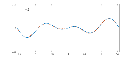
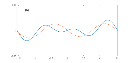
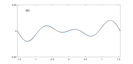
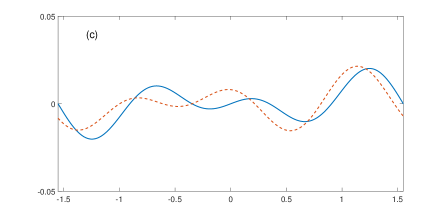
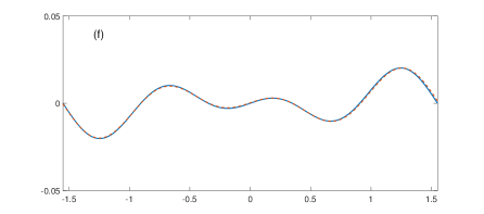
Figure 2. Example 1: the reconstructed surface (dashed line) is plotted against the exact surface (solid line). (a) $\rho_{1}=1$; (b) $\rho_{1}=2$; (c) $\rho_{1}=4$; (d) 1 step of nonlinear correction when $\rho_{1}=4$; (e) 2 steps of nonlinear correction when $\rho_{1}=4$; (f) 3 steps of nonlinear correction when $\rho_{1}=4$.

Example 2. Consider the following surface profile function in the interval $[-1,1]$:

$$g(x)=\begin{cases}1-\cos(2\pi x),\quad&-1\leq x<0,\\ 0.5-0.5\cos(2\pi x),\quad&0<x\leq 1.\\ \end{cases}$$

The period $\Lambda=2$. Although this function is continuous, it is not smooth since the first derivative is not continuous at $x=0$. Figure (3) shows the reconstructed surface (dashed line) against the exact surface (solid line) for different density $\rho_{1}$ and the first three steps of the nonlinear correction. The similar conclusions can be drawn as those for Example 1: the density $\rho_{1}$ helps the resolution and the nonlinear correction improve the reconstruction.

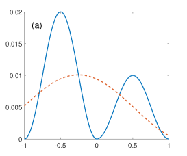
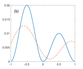
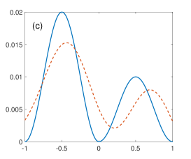
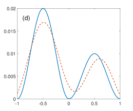
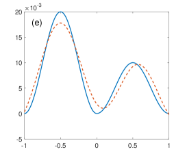
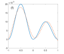
Figure 3. Example 2: the reconstructed surface (dashed line) is plotted against the exact surface (solid line). (a) $\rho_{1}=1$; (b) $\rho_{1}=2$; (c) $\rho_{1}=4$; (d) 1 step of nonlinear correction when $\rho_{1}=4$; (e) 2 steps of nonlinear correction when $\rho_{1}=4$; (f) 3 steps of nonlinear correction when $\rho_{1}=4$.

10. Conclusion

In this paper, we have proposed an effective mathematical model and developed an efficient numerical method to solve the inverse elastic surface scattering problem by using the far-field data. The key idea is to utilize a slab with larger density to allow more propagating modes to propagate to the far-field zone, which contributes to the reconstruction resolution. The nonlinear correction improves the accuracy by using the initial guess generated from the explicit reconstruction formula. Results show that the proposed method is robust to the data noise. The proposed approach can be extended to bi-periodic structures where the three-dimensional Maxwell and elastic equations should be considered. We are investigating these equations and will report the progress elsewhere.

Appendix A second order equations

Consider the final value problem of the second order equation in the interval $(b,a)$:

$$u^{\prime\prime}+\eta^{2}u=0,\quad b<y<a,$$ (A.1a)

$$u=p,\quad y=a,$$ (A.1b)

$$u^{\prime}-{\rm i}\beta u=q,\quad y=a,$$ (A.1c)

where $0\neq\eta,\beta,p,q$ are constants.

Lemma A.1.

The final value problem (A.1) has a unique solution which is given by

$$u(y)=\left(\frac{(\eta+\beta)p-{\rm i}q}{2\eta}\right)e^{-{\rm i}\eta(a-y)}+\left(\frac{(\eta-\beta)p+{\rm i}q}{2\eta}\right)e^{{\rm i}\eta(a-y)}.$$

Proof.

The general solution of the homogeneous second order equation (A.1a) is

$$u(y)=c_{1}e^{{\rm i}\eta y}+c_{2}e^{-{\rm i}\eta y},$$

where $c_{1}$ and $c_{2}$ are constant coefficients to be determined. It follows from the final conditions (A.1b)–(A.1c) that

$$u=p,\quad u^{\prime}={\rm i}\beta p+q,\quad y=a.$$

Plugging the final values of $u$ and $u^{\prime}$ into the general solution, we obtain

$$c_{1}=\left(\frac{(\eta+\beta)p-{\rm i}q}{2\eta}\right)e^{-{\rm i}\eta a},\quad c_{2}=\left(\frac{(\eta-\beta)p+{\rm i}q}{2\eta}\right)e^{{\rm i}\eta a},$$

which completes the proof. ∎

Consider the two-point boundary value problem of the second order equation in the interval $(0,h)$:

$$u^{\prime\prime}+\beta^{2}u=v,\quad 0<y<h,$$ (A.2a)

$$u^{\prime}=r,\quad y=0,$$ (A.2b)

$$u^{\prime}-{\rm i}\beta u=s,\quad y=h,$$ (A.2c)

where $0\neq\beta,r,s$ are constants.

Lemma A.2.

The two-point boundary value problem (A.2) has a unique solution which is given by

$$u(y)=K_{1}(y;\beta)r-K_{2}(y;\beta)s+\int_{0}^{h}K_{3}(y,z;\beta)v(z){\rm d}z,$$

where

$$K_{1}(y;\beta)=\frac{e^{{\rm i}\beta y}}{{\rm i}\beta},\quad K_{2}(y;\beta)=\frac{e^{{\rm i}\beta h}}{2{\rm i}\beta}(e^{{\rm i}\beta y}+e^{-{\rm i}\beta y}),$$

and

$$K_{3}(y,z;\beta)=\begin{cases}\frac{e^{{\rm i}\beta y}}{2{\rm i}\beta}(e^{{\rm i}\beta z}+e^{-{\rm i}\beta z}),\quad z<y,\\[5.0pt] \frac{e^{{\rm i}\beta z}}{2{\rm i}\beta}(e^{{\rm i}\beta y}+e^{-{\rm i}\beta y}),\quad z>y.\end{cases}$$

Proof.

A fundamental set of solutions for the second order equation (A.2a) is

$$u_{1}(y)=e^{{\rm i}\beta y},\quad u_{2}(y)=e^{-{\rm i}\beta y}.$$

A simple calculation yields that the Wronskian $W(u_{1},u_{2})=-2{\rm i}\beta$. It follows from the variation of parameters that the general solution to the nonhomogeneous second order equation (A.2a) is

$$u(y)=c_{1}e^{{\rm i}\beta y}+c_{2}e^{-{\rm i}\beta y}+\frac{e^{{\rm i}\beta y}}{2{\rm i}\beta}\int_{0}^{y}e^{-{\rm i}\beta z}v(z){\rm d}z-\frac{e^{-{\rm i}\beta y}}{2{\rm i}\beta}\int_{0}^{y}e^{{\rm i}\beta z}v(z){\rm d}z,$$ (A.3)

where $c_{1}$ and $c_{2}$ are undetermined constants.

Taking the derivative of (A.3), evaluating at $y=0$, and using the boundary condition (A.2b) give

$$u^{\prime}(0)={\rm i}\beta(c_{1}-c_{2})=r.$$ (A.4)

It follows from the boundary condition (A.2c) that

$$c_{2}=\frac{1}{2{\rm i}\beta}\left(\int_{0}^{h}e^{{\rm i}\beta z}v(z){\rm d}z-se^{{\rm i}\beta h}\right).$$ (A.5)

Combining (A.4) and (A.5) yields

$$c_{1}=c_{2}+\frac{r}{{\rm i}\beta}=\frac{1}{2{\rm i}\beta}\left(\int_{0}^{h}e^{{\rm i}\beta z}v(z){\rm d}z-se^{{\rm i}\beta h}\right)+\frac{r}{{\rm i}\beta}.$$ (A.6)

Substituting (A.5) and (A.6) into (A.3), we obtain the solution. ∎

References

• [1] C. Alves and H. Ammari, Boundary integral formulae for the reconstruction of imperfections of small diameter in an elastic medium, SIAM J. Appl. Math., 62 (2001), 94–106.
• [2] H. Ammari and H. Kang, Reconstruction of small inhomogeneities from boundary measurements, vol. 1846, Lecture Notes in Mathematics, Springer-Verlag, Berlin, 2004.
• [3] H. Ammari, H. Kang, G. Nakamura, and K. Tanuma, Complete asymptotic expansions of solutions of the system of elastostatics in the presence of an inclusion of small diameter and detection of an inclusion, J. Elasticity, 67 (2002), 97–129.
• [4] T. Arens, A new integral equation formulation for the scattering of plane elastic waves by diffraction gratings, J. Integral Equations Appl., 11 (1999), 275–297.
• [5] T. Arens, The scattering of plane elastic waves by a one-dimensional periodic surface, Math. Methods Appl. Sci., 22 (1999), 55–72.
• [6] G. Bao, T. Cui, and P. Li, Inverse diffraction grating of maxwell’s equations in biperiodic structures, Opt. Express, 22 (2014), 4799–4816.
• [7] G. Bao and P. Li, Near-field imaging of infinite rough surfaces, SIAM J. Appl. Math., 73 (2013), 2162–2187.
• [8] G. Bao and P. Li, Convergence analysis in near-field imaging, Inverse Problems, 30 (2014), 085008.
• [9] G. Bao and P. Li, Near-field imaging of infinite rough surfaces in dielectric media, SIAM J. Imaging Sci., 7 (2014), 867–899.
• [10] G. Bao, P. Li, and Y. Wang, Near-field imaging with far-field data, Appl. Math. Lett., 60 (2016), 36–42.
• [11] M. Bonnet and A. Constantinescu, Inverse problems in elasticity, Inverse Problems, 21 (2005), R1–R50.
• [12] O. P. Bruno and F. Reitich, Numerical solution of diffraction problems: a method of variation of boundaries, J. Opt. Soc. Am. A, 10 (1993), 1168–1175.
• [13] A. Charalambopoulos, D. Gintides, and K. Kiriaki, On the uniqueness of the inverse elastic scattering problem for periodic structures, Inverse Problems, 17 (2001), 1923–1935.
• [14] T. Cheng, P. Li, and Y. Wang, Near-field imaging of perfectly conducting grating surfaces, J. Opt. Soc. Am. A, 30 (2013), 2473–2481.
• [15] D. Colton and R. Kress, Inverse acoustic and electromagnetic scattering theory, Springer, New York, 2013.
• [16] D. Courjon, Near-Field Microscopy and Near-Field Optics, Imperial College Press, London, 2003.
• [17] J. Elschner and G. Hu, Variational approach to scattering of plane elastic waves by diffraction gratings, Math. Methods Appl. Sci., 33 (2010), 1924–1941.
• [18] J. Elschner and G. Hu, An optimization method in inverse elastic scattering for one-dimensional grating profiles, Commun. Comput. Phys., 12 (2012), 1434–1460.
• [19] J. Elschner and G. Hu, Scattering of plane elastic waves by three-dimensional diffraction gratings, Math. Models Methods Appl. Sci., 22 (2012), 1150019.
• [20] G. Hu, Y. Lu, and B. Zhang, The factorization method for inverse elastic scattering from periodic structures, Inverse Problems, 29 (2013), 115005.
• [21] X. Jiang and P. Li, Inverse electromagnetic diffraction by biperiodic dielectric gratings, Inverse Problems, 33 (2017), 085004.
• [22] P. Li and J. Shen, Analysis of the scattering by an unbounded rough surface, Math. Methods Appl. Sci., 35 (2012), 2166–2184.
• [23] P. Li and Y. Wang, Near-field imaging of interior cavities, Commun. Comput. Phys., 17 (2015), 542–563.
• [24] P. Li and Y. Wang, Near-field imaging of obstacles, Inverse Probl. Imaging, 9 (2015), 189–210.
• [25] P. Li, Y. Wang, and Y. Zhao, Inverse elastic surface scattering with near-field data, Inverse Problems, 31 (2015), 035009.
• [26] P. Li, Y. Wang, and Y. Zhao, Convergence analysis in near-field imaging for elastic waves, Appl. Anal., 95 (2016), 2339–2360.
• [27] P. Li, Y. Wang, and Y. Zhao, Near-field imaging of biperiodic surfaces for elastic waves, J. Comput. Phys., 324 (2016), 1–23.
• [28] A. Malcolm and D. P. Nicholls, A field expansions method for scattering by periodic multilayered media, J. Acoust. Soc. Am., 129 (2011), 1783–1793.
• [29] D. P. Nicholls and F. Reitich, Shape deformations in rough-surface scattering: cancellations, conditioning, and convergence, J. Opt. Soc. Am. A, 21 (2004), 590–605.
• [30] D. P. Nicholls and F. Reitich, Shape deformations in rough-surface scattering: improved algorithms, J. Opt. Soc. Am. A, 21 (2004), 606–621.