A simple ansatz for the study of velocity autocorrelation functions in fluids at different timescales

Abstract

A simple ansatz for the study of velocity autocorrelation functions in fluids at different timescales is proposed. The ansatz is based on an effective summation of the infinite continued fraction at a reasonable assumption about convergence of relaxation times of the higher order memory functions, which have a purely kinetic origin. The VAFs obtained within our approach are compared with the results of the Markovian approximation for memory kernels. It is shown that although in the ‘‘overdamped’’ regime both approaches agree to a large extent at the initial and intermediate times of the system evolution, our formalism yields power law relaxation of the VAFs which is not observed at the description with a finite number of the collective modes. Explicit expressions for the transition times from kinetic to hydrodynamic regimes are obtained from the analysis of the singularities of spectral functions in the complex frequency plane.

Key words: nonequilibrium statistical mechanics, statistical hydrodynamics, classical fluids, Langevin equation, Markovian processes

PACS: 05.20.Jj, 47.10.-g, 47.11.-j

Abstract

Запропоновано простий анзац для дослiдження автокореляцiйних функцiй швидкостей (АФШ) флюїду на рiзних часових промiжках, що базується на ефективному пересумуваннi безмежних ланцюгових дробiв на основi фiзично обгрунтованого припущення про збiжнiсть часiв релаксацiї ядер вищих порядкiв, якi мають суто кiнетичну природу. Отриманi в рамках такого анзацу АФШ порiвнюються з результатами маркiвського наближення для вiдповiдних функцiй пам’ятi. Показано, що хоча в передемпферованому режимi обидва пiдходи дають дуже близькi результати на малих та промiжних часах, лише метод пересумовування дробiв веде до появи степеневих законiв у поведiнцi АФШ на великих часах, що не спостерiгається при описi динамiки флюїду скiнченним числом колективних мод. На основi аналiзу сингулярностей спектральних функцiй на комплекснiй площинi частот отриманi явнi вирази для оцiнки часiв переходу вiд кiнетичного етапу еволюцiї флюїду до гiдродинамiчного режиму.

Ключовi слова: нерiвноважна статистична механiка, статистична гiдродинамiка, класичнi флюїди, рiвняння Ланжевена, маркiвськi процеси

1 Introduction

The dynamics of many-body systems at various time scales remains as one of the main problems of the non-equilibrium statistical mechanics despite its long history and considerable achievements obtained so far. Systematic studies of the time behaviour of condensed matter systems started with the pioneering work by Bogoluyubov [1], where a concept of the weakening correlations allowed one to reformulate a completely unsolvable problem of the $N$-body dynamics into a much more manageable task in terms of the correlation functions of lower orders $s\ll N$.

Within such an approach, a time hierarchy of the physical stages, through which the system passed during its evolution toward equilibrium (starting from the kinetic stage via intermediate steps till the hydrodynamic one and beyond [2]), appears quite naturally. The corresponding time scales within that hierarchy can serve as a basis for generalized hydrodynamics, in particular, in generalized collective mode theory (GCM) [3, 4], where the set of dynamical variables for description of long- and short-time correlations usually consists of the densities of conserved quantities and their time derivatives up to a certain order. Using a physically reasonable assumption in the Markovian approximation [5] for the kinetic kernels of higher orders, one actually comes to a simple mathematical problem, expressing collective processes in the system in terms of the dynamic eigenmodes: complex/real eigenvalues for propagating/relaxing processes and corresponding eigenvectors which characterize contribution of particular eigenmode to relevant correlations. A definite advantage of the GCM is the fact that such a theory is a computer adapted one: all the elements of the generalized dynamic matrix could be expressed via the static correlation functions (SCF) and corresponding relaxation times, which can be obtained by molecular dynamic simulations [5, 6].

Although the GCM can be extended by taking into account the ‘‘ultraslow’’ processes (defined by the time integrals of corresponding densities [7, 8, 9]), the problems of account for slow structural relaxation [10] are usually approached by theories with non-local coupling of dynamic variables. In the framework of the mode coupling theory (MCT) [11], a basic set of the dynamic variables consists of higher products [12] rather than of higher derivatives of the densities of conserved quantities. Like in the GCM, a time/spatial dispersion of the kinetic kernels of lower orders gives rise to some peculiarities of time correlation functions (TCF). However, in contrast to the GCM, where the system description at long times is a ‘‘bottleneck’’ of the theory, the MCT approach manifests its efficiency upon the hydrodynamic stage of the system evolution yielding the $t^{-D/2}$ power law for the TCFs [13]. Recently [14], the basic ideas of MCT have been used to obtain a mean field approximation for the memory kernels, and to study a slow dynamics of some soft matter systems like molecular liquids or colloid suspensions. Such an approach was shown to yield reasonable results in the whole time scale: from the ballistic motion of a separate molecule to the diffusion regime.

Another approach that incorporates some advantages of both theories mentioned above has been proposed in the papers [15, 16]. The authors have used the continued fraction method for the Laplace transforms of the VAFs and reasonable approximations for the memory kernels at the stage of the closure procedure with subsequent profound analysis of the VAF peculiarities at the complex frequency plane. It was shown that unlike the GCM case, characterized by a limited number of the isolated poles, VAF shows the singularity manifold forming branch cuts. The branch cuts were found to be separated from the real axis by the well-defined ‘‘gap’’. The inverse value of the gap width determines a duration of the transition period from the short-time one-particle kinetics to the long-time collective motion (hydrodynamics) with a typical power law relaxation $\sim t^{-3/2}$ of the VAFs, which has been reported for the first time and explained by Alder and Wainwright in [17]. According to [17], the long-time tails of VAF are sustained by neighbour backflow created by redistribution of momentum of the moving particle with neighbour particles.

Very recently, a microscopic interpretation of the long-time tails of VAF was suggested from the analysis of its memory kernel [18]. It was shown, that the hydrodynamically added mass, defined via memory kernel, has a negative sign, and the backflow of neighbours tends to drag the particle in the direction of its initial velocity, i.e., contributes negatively to the friction.

There are also some other approaches to study the system dynamics, which are not directly related to the concept of the weakening correlations, or to the corresponding time hierarchy. Within the Langevin formalism [19], a tagged particle is postulated to interact with its neighbourhood as with a thermal bath, which possesses certain spectral properties. In the framework of the Mittag-Leffler generalization [20] of the Langevin approach, a correlation function of the random noises behaves as a stretched exponential for the short times and as an inverse power law at the long-time scale. This allows one to describe different dynamical regimes of the particle motion such as oscillations and negative correlations of the VAFs, depending on the parameters of the Mittag-Leffler function.

Summarizing all the above mentioned — in spite of the considerable achievements in exploration of dynamics of many-particle systems — there is still a lack of the unified self-consistent approaches being able to describe the systems behaviour throughout all the stages of evolution. An attempt to create such an approach is the motivation of our paper. In our studies we i) present our viewpoint on peculiarities of the fluid dynamics at different time scales; ii) establish the reasons of the ‘‘long tails’’ origin in the VAFs; and iii) investigate a crossover from the kinetics to the hydrodynamics.

Our approach incorporates basic ideas of the GCM [3, 4, 5], MCT [11, 12, 13, 14], the formalism of continued fractions for the time correlation functions [21, 22], and the method of the TCFs analysis on the plane of complex frequency elaborated in [15, 16]. To be specific, we consider the VAF as a particular case of the more general TCF and use a continued fraction representation for its Laplace transforms. In such an approach, there appears a set of SCFs dealt with a force acting on the particle and its higher derivatives. These SCFs serve as the control parameters $\Gamma_{i}$ to be evaluated, for instance, from computer simulations. A cornerstone of our scheme is an effective summation of infinite continued fractions, based on a quite reasonable (and physically grounded) assumption about a convergence of relaxation times of the higher modes [23, 24] of purely kinetic origin. This allows us to obtain an explicit expression for the memory kernel of the highest order, which turned out to be oscillatory in time representation and decays as $t^{-3/2}$.

We show that at a wide enough domain of the control parameters $\Gamma_{i}$, the VAFs, calculated within our approach, almost coincide at the initial and intermediate times with those obtained in the framework of the finite modes approximation. However, in contrast to the GCM, which implies a description by the set of exponents and does not permit the ‘‘long tails’’ to appear at the hydrodynamic stage of the system evolution, we obtain a specific $\sim t^{-3/2}$ relaxation (or even slower decay $\sim t^{-1/2}$ at a certain critical value of the parameter $\Gamma_{i}$). At the same time, if we fix a level $s$, where the summed up kinetic kernel is located, we can provide the frequency moments up to the $2s$-th order as well as the zeroth time moment of the VAF to obey the ‘‘sum rules’’ [4, 5, 6], like it holds within the GCM framework.

In addition, we show that a transition time from the exponential relaxation at the intermediate stage of the system evolution to the power law decay at the hydrodynamic stage depends on the distance of the corresponding singularities of the spectral functions from the coordinate origin. Our results are in a close agreement with the conclusions of [15, 16], though the starting point of our approach differs from the basic assumptions of the cited papers.

A structure of the paper is as follows. In section 2, we briefly recall the method of continued fractions for the VAF presentation, and calculate the memory function of the highest order at the assumption mentioned above. In section 3, we evaluate the spectral functions both by the effective summation of the continued fraction and in the finite modes approximation. In section 4, an analysis of the VAFs dynamics is performed. The VAFs are shown to behave in a solid-like, gas-like or liquid-like manner depending on the control parameters $\Gamma_{i}$. A special attention will be paid to the case when the fluid behaves as an effective $1\text{D}$ system with typical $\sim t^{-1/2}$ decay at long times. In section 5, we investigate in detail a transition of the VAFs to the power law asymptotics. Finally, we draw the conclusions in section 6.

2 Continued fraction representation for velocity autocorrelation function

Let us consider the normalized VAF

$$F_{v}(t)=\langle\textbf{v}_{i}\exp(-\textrm{i}L_{N}t)\textbf{v}_{i}\rangle/\langle\textbf{v}_{i}\textbf{v}_{i}\rangle,$$ (2.1)

where $\textrm{i}L_{N}$ means the Liouville operator. For the system of structureless particles interacting via the central force potential it has a very simple form [2], being dependent on positions and momenta of all the particles.

The Laplace-transformed VAF as a formal solution of the generalized Langevin equation reads

$$\tilde{F}_{v}(z)=\frac{1}{z+\tilde{\phi}_{1}(z)}~{},$$

where $\phi_{0}(z)$ is the Laplace-component of the lowest-order memory kernel which should contain all the information on the dissipation processes in a fluid, an explicit expression for which should be obtained from the higher-order memory kernel $\phi_{s}(z)$, which satisfies a recurrence relation [25]

$$\tilde{\phi}_{s-1}(z)=\frac{\Gamma_{s-1}}{z+\tilde{\phi}_{s}(z)}\,,$$ (2.2)

where $\Gamma_{s-1}$ is the relevant SCF. It is possible to present the equation for the Laplace transform $\tilde{F}_{v}(z)$ of VAF (2.1) as an infinite continued fraction

$$\tilde{F}_{v}(z)=\displaystyle\displaystyle\frac{1}{z+\displaystyle\frac{\Gamma_{1}}{z+\displaystyle\frac{\Gamma_{2}}{z+\displaystyle\frac{\Gamma_{3}}{z+\cdots}}}}\,.$$ (2.3)

All the parameters $\Gamma_{i}$ entering (2.3) are expressed according to a general definition [25] via the ‘‘force-force’’ SCFs and its higher derivatives. The lowest order SCFs can be presented as follows:

$$\Gamma_{1}=\frac{\langle\mathbf{F}_{i}\mathbf{F}_{i}\rangle}{\langle\mathbf{v}_{i}\mathbf{v}_{i}\rangle}=\frac{\beta}{3m}\langle\mathbf{F}_{i}\mathbf{F}_{i}\rangle,\qquad\Gamma_{2}=\frac{\langle{\textrm{i}L_{N}\mathbf{F}_{i}\textrm{i}L_{N}\mathbf{F}_{i}}\rangle}{\langle\mathbf{F}_{i}\mathbf{F}_{i}\rangle}-\Gamma_{1}.$$ (2.4)

To evaluate the static correlators $\Gamma_{1}$, one should obtain a pair correlation function of the fluid at a given thermodynamic point. The SCF $\Gamma_{2}$ would require the knowledge of even higher order correlation functions, which yields the problem completely unmanageable. Therefore, such a structural analysis of the fluid could not be considered as a promising one, and reliable results for VAFs as well as for higher order SCFs $\Gamma_{i}$ should be obtained only by MD simulation. Any theoretical approximation should be compared with the MD data to verify an efficiency of the chosen approach.

The infinite continued fraction (2.3) can be rewritten [21] as a weighted sum

$$\tilde{F}_{v}(z)=\sum\limits_{j=1}^{\infty}\frac{I_{j}}{z-z_{j}}\,,$$ (2.5)

where $I_{j}$ denote the amplitudes of particular $j$-th mode of the fluid, whereas $z_{j}$ mean the mode frequencies. In the framework of GCM [5, 26], these values can be calculated by solving the eighenvalues/eighenvectors problem for the generalized dynamic matrix of the infinite dimension, while in the other approach [21, 22] they are taken as fitting parameters. In fact, an evaluation of all the higher order correlators $\Gamma_{i}$ is not a realistic task. Therefore, for practical purposes one should truncate the series (2.5), retaining only a limited number $M$ of terms. In accordance with the basic concept of GCM, it corresponds to the $M$ modes contribution to the VAF.

For instance, limiting ourselves by two terms in (2.5) (this corresponds to the Markovian approximation $\tilde{\phi}_{2}(z)\approx\tilde{\phi}_{2}(0)$ for the second order memory kernel), and writing down

$$\tilde{\phi_{1}}(z)\approx\frac{\Gamma_{1}}{z+\tilde{\phi}_{2}(0)}\,,$$ (2.6)

we can reproduce equation (15) of [6] for the VAF of a simple fluid. Such a model admits the existence of either two purely relaxing or two propagating modes in the VAF dynamics, depending on the relation between two typical times of the system evolution. These times are: i) duration of the hydrodynamic processes connected with the self-diffusion, and ii) the inverse Einstein frequency.

We have already mentioned that construction of the exact representation of VAF as an infinite continued fraction (2.3) seems to be an unrealistic problem. We note that a truncation of the series (2.5) even at a large number of terms may perturb the VAF’s dynamics. This distortion can be insignificant (allowing one to describe the system dynamics at small and intermediate times in the GCM framework) or essential (not allowing one to study a hydrodynamic regime of the system evolution). However, even in the first case, the issue of truncation of the series (2.5) to approximate the VAF by a finite number of modes as accurately as possible should be solved separately for each particular system and for each particular thermodynamic point [22]. As regards the second case, from a strictly mathematical viewpoint there is not another reason of the power law behaviour of the VAFs at long times than a contribution of the infinite number of terms in (2.3). In the MCT approach [11, 12], which is not directly related to a truncation of the continued fractions, the system dynamics is modelled at the long times but could fail at the other timescales.

Therefore, we propose to adopt another approach for an approximate evaluation of the infinite continued fraction (2.3). The Markovian approximation of the lowest order kinetic kernel is known to determine [26] the relaxation time $\tau_{1}$ of the corresponding hydrodynamic excitation by a simple relation $\tilde{\phi}_{1}(0)=\tau_{1}^{-1}$. Introducing in a similar manner the $s$-th order relaxation times, and using a fact [24, 26] that the relaxation times of the higher modes become comparable with each other and tend to a certain fixed value, which is of a purely kinetic origin, we can put this assumption for large enough $s$ into an explicit form,

$$\tilde{\phi}_{s}(0)\approx\tilde{\phi}_{s+1}(0)\approx\tilde{\phi}_{s+2}(0)=\ldots.$$ (2.7)

Keeping in mind equation (2.7) and making use of the relation (2.2), where the condition $\tilde{\phi}_{s}(0)=\tilde{\phi}_{s+1}(0)$ is used, one can obtain a simple expression for the $s$-th order memory function in the Markovian approximation,

$$\tilde{\phi}_{s}(0)\approx\sqrt{\Gamma_{s}}\,.$$ (2.8)

It also follows from equations (2.2)–(2.7) that all the higher order SCFs $\Gamma_{i}$, $i=\{s,s+1,\ldots\}$, are almost equal to each other,

$$\Gamma_{s}=\Gamma_{s+1}=\Gamma_{s+2}=\ldots,$$ (2.9)

whereas the remaining SCFs with $2i+1<s$ yield the recurrence relations for the corresponding relaxation times,

$$\frac{1}{\tau_{2i}}=\frac{1}{\tau_{2i-1}}\sqrt{\frac{\Gamma_{2i}}{\Gamma_{2i+1}}}\,,\qquad\frac{1}{\tau_{2i+1}}=\frac{1}{\tau_{2i}}\sqrt{\frac{\Gamma_{2i+2}}{\Gamma_{2i+1}}}\,.$$ (2.10)

One can see from equation (2.10) that there are, actually, two sets of relations for the odd and the even $i$, separately. It is known from the theory of continued fractions [27] as well as from the analysis of fluid dynamics [24] that $\tau_{i}$ oscillates around a certain value $\tau^{*}$, approaching this asymptotics from below (the odd order relaxation times) or above (the even order relaxation times). Moreover, the difference between $\tau_{2i}$ and $\tau_{2i+1}$ decreases rapidly with increasing $i$.

If one assumes $\tau_{s}$ to reach its asymptotics instantly [this, in fact, corresponds to approximation (2.7)], the recurrence relation (2.2) reduces to a bilinear form

$$\tilde{\phi}_{s}(z)=\frac{\Gamma_{s}}{z+\tilde{\phi}_{s}(z)}\,,$$ (2.11)

hence, an explicit expression for the $s$-th order memory kernel can be easily obtained,

$$\tilde{\phi}_{s}(z)=-\frac{z}{2}+\sqrt{\frac{z^{2}}{4}+\Gamma_{s}}\,.$$ (2.12)

This result looks quite interesting if one performs the inverse Laplace transformation to (2.12),

$$\phi_{s}(t)\equiv\frac{1}{2\piup\textrm{i}}\lim\limits_{\epsilon\to 0}\!\!\int\limits_{\epsilon-\textrm{i}\infty}^{\epsilon+\textrm{i}\infty}\!\!\!\textrm{e}^{zt}\tilde{\phi}_{s}(z)\mathrm{d}z=\sqrt{\Gamma_{s}}\,\,\frac{J_{1}\big{(}2\sqrt{\Gamma_{s}}t\big{)}}{t}\,.$$ (2.13)

It means that the $s$-th order memory kernels decay non-monotonously at long times as $t^{-3/2}$ since the Bessel function of the first order $J_{1}$, entering equation (2.13), obeys the well known asymptote $J_{1}(x\gg 1)=\sqrt{\frac{2}{\piup x}}\cos\left(x-3\piup/4\right)$.

Equations (2.12)–(2.13), obtained in the framework of the rigorous approach using just one physically reasonable assumption (2.7), are the cornerstones for our further study of the VAFs dynamics. In the next section we consider the spectral functions with various values $s$, at which the condition (2.7) starts to hold true. These results are compared with the finite continued fraction approach, for which the corresponding Markovian approximation yields the expression

$$\tilde{\phi}_{s-1}(z)\approx\frac{\Gamma_{s-1}}{z+\tilde{\phi}_{s}(0)}=\frac{\Gamma_{s-1}}{z+\sqrt{\Gamma_{s}}}$$ (2.14)

for the $(s-1)$-th order memory function.

Later on, we perform an inverse Fourier transformation to obtain a time representation $F_{v}(t)$ of the corresponding VAFs and to show that even two levels of the hierarchy, at which the summed up kinetic kernel (2.12) is located, allow the VAFs to mimic a ‘‘gas-like’’, ‘‘liquid-like’’ or ‘‘solid-like’’ behaviour of the simple fluid depending on the interplay between the SCFs $\Gamma_{i}$. An essential feature is the appearance of long time tails of the VAFs, which cannot be obtained within GCM.

3 Spectral functions

Before representing the VAF by means of the summed up continued fraction $(\ref{phiS_result})$, one can ask a natural question: what level $s$ can be considered as a sufficient one for the higher order memory kernels $\tilde{\phi}_{s}(0)$ in order to reach their asymptotic value and the relation (2.7) to be true? This would require sophisticated calculations of the sequence of SCFs by computer simulations. However, to obtain some analytical estimates, in this section we assume that the condition (2.7) is valid starting from quite low values $s\geqslant 2$.

Let us consider the spectral function (SF) $\tilde{F}_{v}(\omega)=\mathop{\symoperators Re}\nolimits\big{[}\tilde{F}_{v}(z=\textrm{i}\omega)\big{]}$, defined as a real part of the corresponding continued fraction (2.3) taken at the imaginary frequency. Hereafter, we replace the label $v$ in the expressions for SFs (and for VAFs) by the subscript $\alpha$ which denotes the chosen level of approximation (for details see below).

If one supposes the following relation

$$\Gamma_{2}=\Gamma_{3}=\ldots=\Gamma_{s}=\ldots$$ (3.1)

to be valid, it is straightforward to evaluate SF $\tilde{F}_{2}(\omega)$:

$$\tilde{F}_{2}(\omega)=\frac{\Gamma_{1}\sqrt{\Gamma_{2}-\omega^{2}/4}}{(\Gamma_{2}-\Gamma_{1})\omega^{2}+\Gamma^{2}_{1}}\,.$$ (3.2)

It is also instructive to compare the result (3.2) with the expression

$$\tilde{F}_{\text{M2}}(\omega)=\frac{\Gamma_{1}\sqrt{\Gamma_{2}}}{\omega^{4}+(\Gamma_{2}-2\Gamma_{1})\omega^{2}+\Gamma_{1}^{2}}$$ (3.3)

for the SF, obtained by a truncation of the continued fraction at the level $s=2$ [or, which is the same, after the Markovian approximation $\tilde{\phi}_{2}(z)\approx\tilde{\phi}_{2}(0)$ for the memory kernel of the 2-nd order]. Hereafter, we use an extra subscript ‘‘M’’ to denote the above mentioned Markovian approximation.

It is useful to compare the expressions (3.2)–(3.3) for the corresponding SFs. First of all, the former spectral function vanishes at the cut-off frequency $\omega_{\textrm{c}}=2\sqrt{\Gamma_{2}}$, while the latter tends to zero asymptotically as $1/\omega^{4}$. Secondly, both SFs are even functions of frequency, and behave as $\lim_{\omega\to 0}\mathrm{d}\tilde{F}_{\alpha}(\omega)/\mathrm{d}\omega=0$, here $\alpha$ denotes 2 or M2. Thirdly, in the domain of frequencies $\omega\ll\omega_{\textrm{c}}$ and at $\Gamma_{1}\ll\Gamma_{2}$, the relation $\tilde{F}_{2}(\omega)\approx\tilde{F}_{\text{M2}}(\omega)$ holds true [to put it more precisely, an exact relation $\tilde{F}_{2}(0)=\tilde{F}_{\text{M2}}(0)$ is valid, see discussion in section 4].

At last, in the vicinity $\varepsilon$ of the cut-off frequency $\omega_{\textrm{c}}$, the SF (3.2) behaves as

$$\tilde{F}_{2}(\omega_{\textrm{c}}-\varepsilon)\approx\frac{\Gamma_{1}\Gamma_{2}^{1/4}}{(\Gamma_{1}-2\Gamma_{2})^{2}}\sqrt{\varepsilon}.$$ (3.4)

The square root dependence (3.4) resembles the well-known result from the MCT [12, 13]. However, in the MCT approach, a non-analytical dependence $\sqrt{\omega}$ of the SFs, generating the long time tails $\sim t^{-3/2}$ of the VAFs, occurs at the low frequency domain rather than at $\omega_{\textrm{c}}$.

A similar structure of the SF can be obtained at the assumption

$$\Gamma_{3}=\Gamma_{4}=\ldots=\Gamma_{s}=\ldots,$$ (3.5)

when all the relaxation times $\tau_{s}$, starting from $s=3$, are supposed to be the same (compare with the condition (3.1)). In this case, the spectral function $\tilde{F}_{3}(\omega)$, obtained by summing up the continued fraction for the 3-rd order memory kernel, can be presented as follows:

$$\tilde{F}_{3}(\omega)=\frac{\Gamma_{1}\Gamma_{2}\sqrt{\Gamma_{3}-\omega^{2}/4}}{(\Gamma_{3}-\Gamma_{2})\omega^{4}+\big{[}\Gamma_{2}(\Gamma_{1}+\Gamma_{2})-2\Gamma_{1}\Gamma_{3}\big{]}\omega^{2}+\Gamma_{1}^{2}\Gamma_{3}}\,,$$ (3.6)

while its counterpart in the modes approximation looks as

$$\tilde{F}_{\text{M3}}(\omega)=\frac{\Gamma_{1}\Gamma_{2}\sqrt{\Gamma_{3}}}{\omega^{6}-\big{[}2(\Gamma_{1}+\Gamma_{2})-\Gamma_{3}\big{]}\omega^{4}+\big{[}(\Gamma_{1}+\Gamma_{2})^{2}-2\Gamma_{1}\Gamma_{3}\big{]}\omega^{2}+\Gamma_{1}^{2}\Gamma_{3}}\,.$$ (3.7)

Like in the the cases (3.2)–(3.3), the two SFs are close to each other, $\tilde{F}_{3}(\omega)\approx\tilde{F}_{\text{M3}}(\omega)$, in the domain of low frequencies $\omega\ll\omega_{\textrm{c}}$ and at $\Gamma_{3}\gg\mbox{max}\{\Gamma_{1},\Gamma_{2}\}$.

It should be stressed that there is a restriction from below for the minimal value $\Gamma_{s}^{(\textrm{min})}$ of the highest order SCF (in our case, $s=2$ or 3), which follows from the sum rule

$$\frac{1}{2\piup}\int\limits_{-\infty}^{\infty}\tilde{F}_{s}(\omega)\mathrm{d}\omega\equiv\frac{1}{2\piup}\int\limits_{-\omega_{\textrm{c}}}^{\omega_{\textrm{c}}}\tilde{F}_{s}(\omega)\mathrm{d}\omega=1.$$ (3.8)

Equation (3.8), in fact, denotes the initial value of the VAF, which is equal (by definition) to the unity. A direct integration of (3.2) shows that at a fixed value $\Gamma_{1}$, the sum rule (3.8) holds true for all $\Gamma_{2}\geqslant\Gamma_{2}^{(\textrm{min})}$, where $\Gamma_{2}^{(\textrm{min})}=\Gamma_{1}/2$.

In a similar way, the value $\Gamma_{3}^{(\textrm{min})}=(\Gamma_{1}+2\Gamma_{2})/4$ can be defined for a fixed lower order SCFs $\Gamma_{1}$, $\Gamma_{2}$ in equation (3.6), and the sum rule (3.8) is satisfied for $\Gamma_{3}\geqslant\Gamma_{3}^{(\textrm{min})}$. In this context, our results differ from those [see equations (3.3), (3.7)] obtained within the modes approximation: in the latter case, no relation between various $\Gamma_{i}$ is needed for the sum rule (3.8) to be satisfied.

We should emphasize that so far the minimal values $\Gamma_{s}^{(\textrm{min})}$ appear in a strictly mathematical way due to the requirement of the sum rule (3.8). Later on, we will try to attribute a more physical meaning for $\Gamma_{s}^{(\textrm{min})}$ (as well as for $\omega_{\textrm{c}}$), when studying the time behaviour of the corresponding VAFs and discussing the process of the long tails formation in section 5.

At the end of this section, we would like to present an expression for spectral weight functions $J(\omega)$, which determine the generalized friction coefficient

$$\gamma(t)=\frac{1}{\piup}\int\limits_{0}^{\infty}\frac{J(\omega)}{\omega}\cos\omega t\,\mathrm{d}\omega,$$ (3.9)

entering the Langevin equation for the tagged particle of the fluid, which is supposed to interact with its neighbourhood as a collection of the $N$ bath modes [19]. Identifying [20] the generalized friction coefficient with the 2-nd order memory kernel (2.13) and taking into account equation (3.9), one can obtain an expression for the spectral weight function as follows:

$$J(\omega)=\frac{4\Gamma_{2}}{\piup\omega_{\textrm{c}}^{2}}\omega\sqrt{\omega_{\textrm{c}}^{2}-\omega^{2}}\,.$$ (3.10)

It is seen from equation (3.10) that the fluid corresponds to the Ohmic system [28], since in the low frequency domain the spectral weight function behaves as $J(\omega)\sim\omega$. The obtained result looks quite expected. However, there is a cut-off frequency $\omega_{\textrm{c}}$ at which $J(\omega)$ abruptly vanishes. In this context, equation (3.10) differs from the commonly accepted form for the spectral weight functions, which are usually expressed as

$$J(\omega)\sim\omega^{n}\exp(-\omega/\omega_{\textrm{c}})$$ (3.11)

with $0\!<\!n\!<\!1$ for the sub-Ohmic systems, $n=1$ for the Ohmic ones, and $n>1$ for the super-Ohmic coupling [28].

It is widely believed that the low frequency asymptote determines the long time behaviour of the corresponding TCF, and the cut-off frequency in the exponent of (3.11) can just slightly change the shape of TCF. However, in the theory of solids, it is reasonable [29, 30] to consider the upper cut-off frequency $\omega_{\textrm{c}}$, associated, for instance, with the Debye frequency $\omega_{\textrm{D}}$, and to put $J(\omega)=0$ at $\omega>\omega_{\textrm{c}}$, like it happens in the case under consideration. An advantage of our approach consists in the fact that the expression (3.10) has been obtained rigorously using the only assumption (3.1) for the SCFs of higher orders, and the cut-off frequency $\omega_{\textrm{c}}$ has appeared in a natural way (not as a fitting parameter). Although from the mathematical standpoint any truncation of the spectral weight function at the finite frequency $\omega_{\textrm{c}}$ generates an oscillating power law behaviour of the corresponding TCF at long times, it is in our approach that a correct asymptotics $t^{-3/2}$ of VAF is ensured.

4 Time behaviour of the VAFs

Expressions (3.2)–(3.3) and (3.6)–(3.7) allow us to study the frequency dependence of SFs in a broad domain of parameters $\Gamma_{s}$ as it has been discussed in section 3. However, it would be more instructive to perform the inverse Fourier transformation of the above mentioned expressions and to consider the dynamics of the corresponding VAFs.

One important remark is to the point. In this section, we consider various values of $\Gamma_{s}$ regardless of their relations to the fluid at a particular thermodynamic point. We reckon our task in presentation of different regimes of the fluids dynamics, modelled in the framework of our approach. Certainly, all these SCFs need a verification by computer simulations. Moreover, it may turn out that some combinations of $\Gamma_{s}$ can even be non-representative for real fluids. Nevertheless, preliminary estimations show that the basic features of the fluids dynamics such as the short time behaviour, the transition regimes, formation of the long tails, etc., presented in this paper, are also valid with $\Gamma_{s}$, obtained in a strict way (by computer simulations at various temperatures and densities).

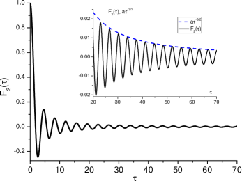
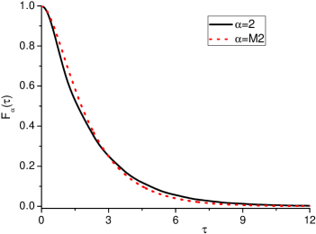
Figure 1: (Colour online) Time evolution of the VAF $F_{2}(\tau)$ (solid line) at $\Gamma_{1}\tau^{2}_{\textrm{LJ}}=1$, $\Gamma_{2}\tau^{2}_{\textrm{LJ}}=0.75$ (left-hand panel) and $\Gamma_{1}\tau^{2}_{\textrm{LJ}}=1$, $\Gamma_{2}\tau^{2}_{\textrm{LJ}}=5$ (right-hand panel). The dotted line corresponds to the VAF in the Markovian approximation (labelled by $\alpha=\text{M2}$). In the inset: the VAF at long times (solid line) and its asymptotics $a\tau^{-3/2}$ (dashed line) with $a=2.1$. The dimensionless value $\tau=t/\tau_{\textrm{LJ}}$ is defined via the typical time $\tau_{\textrm{LJ}}=\sigma_{\textrm{LJ}}\sqrt{m/\varepsilon_{\text{LJ}}}$ of the Lennard-Jones system.

We begin our investigation using approximation (3.1). In figure 1 we present the time behavior of the VAFs calculated at two different parameters $\Gamma_{2}$ whereas $\Gamma_{1}$ is chosen to be fixed. It could be said (see the left-hand panel of figure 1) that at small values of $\Gamma_{2}$, the VAF shows a solid-like [31] behaviour since there are well defined oscillations in the whole time domain, which decay as $at^{-3/2}$ at long times, as it is shown by the dashed line. The parameter $a$ is nothing but a fraction in the expansion (3.4) divided by $\sqrt{\piup}$. Obviously, we are not dealing with a real solid: the oscillations are damped, and the area under the curve, which determines the self-diffusion coefficient, differs from zero [it also follows from the inequality $\tilde{F}_{2}(0)\neq 0$, see equation (3.2)].

At a larger value of $\Gamma_{2}$, the VAF behaves in a gas-like manner. In a gas, the molecules are not confined by intermolecular bonding, and the VAF decays without any oscillation. In our case, there is a smooth relaxation of $F_{2}(t)$ at the initial and at intermediate times. It is worthy to point out that the two modes approximation $F_{\text{M2}}(t)$ yields a very similar result (see the dotted line in figure 1), as it has been mentioned in section 3.

This close resemblance becomes even more reasonable if one notices that both approaches ensure an equality of the frequency moments $\langle\omega_{\alpha}^{m}\rangle=\frac{1}{2\piup}\int_{-\infty}^{\infty}\omega^{m}\tilde{F}_{\alpha}(\omega)\mathrm{d}\omega$ of the low orders,

$$\left\langle\omega^{0}_{2}\right\rangle=\left\langle\omega^{0}_{\text{M2}}\right\rangle=1,$$

$$\left\langle\omega^{2}_{2}\right\rangle=\left\langle\omega^{2}_{\text{M2}}\right\rangle=\Gamma_{1}\,,$$

$$\left\langle\omega^{4}_{2}\right\rangle=\Gamma_{1}(\Gamma_{1}+\Gamma_{2}),\qquad\left\langle\omega^{4}_{\text{M2}}\right\rangle=\infty.$$ (4.1)

It should be also mentioned that the higher order frequency moments obtained within the Markovian approximation diverge [see the last row in equation (4)] whereas all the frequency moments in our scheme are finite being calculated by integration over the finite interval $[-\omega_{\textrm{c}},\omega_{\textrm{c}}]$.

A similar equality,

$$\left\langle\tau^{0}_{2}\right\rangle=\left\langle\tau^{0}_{\text{M2}}\right\rangle=\frac{\sqrt{\Gamma_{2}}}{\Gamma_{1}}\,,$$ (4.2)

can be obtained for the zeroth time moment $\left\langle\tau_{\alpha}^{0}\right\rangle=\int_{0}^{\infty}F_{\alpha}(t)\mathrm{d}t$, which defines a self-diffusion coefficient of the fluid. The higher order time moments (starting from $s\geqslant 2$), obtained in our approach, diverge due to the long tail formation (see the inset in the left-hand panel of figure 1).

If $\Gamma_{2}$ is much greater than $\Gamma_{1}$, as it occurs in the diluted fluids and is confirmed by MD, the power law regime can be formally set at the infinitely large times, which are not accessible by the computer simulation [for estimation of the transition times see equation (5.8) in section 5]. The oscillations with a vanishing amplitude along with the envelope curve $at^{-3/2}$ (not shown in the right-hand panel of figure 1) cannot, in fact, be observed. Therefore, there is not a controversy between the predicted power law behaviour of the VAFs, modulated by the high frequency $\omega_{\textrm{c}}$ at long times, and the non-reversed motion of the gas particles at the whole time domain.

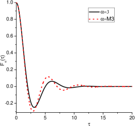
Figure 2: (Colour online) Time evolution of the VAF $F_{3}(\tau)$ (solid line) at $\Gamma_{1}\tau^{2}_{\textrm{LJ}}=1$, $\Gamma_{2}\tau^{2}_{\textrm{LJ}}=1.5$, $\Gamma_{3}\tau^{2}_{\textrm{LJ}}=1.05$ (left-hand panel), $\Gamma_{1}\tau^{2}_{\textrm{LJ}}=1$, $\Gamma_{2}\tau^{2}_{\textrm{LJ}}=1.5$, $\Gamma_{3}\tau^{2}_{\textrm{LJ}}=1.7$ (central panel) and $\Gamma_{1}\tau^{2}_{\textrm{LJ}}=1$, $\Gamma_{2}\tau^{2}_{\textrm{LJ}}=1.5$, $\Gamma_{3}\tau^{2}_{\textrm{LJ}}=4$ (right-hand panel). The dotted line corresponds to the VAF in the Markovian approximation (labelled by $\alpha=\text{M3}$).

The fluid dynamics becomes more diverse if one accepts the approximation (3.5) to be valid. In this case, the corresponding VAFs depend on three SCF $\Gamma_{i}$, $i=\{1,2,3\}$. It is seen from the right-hand panel of figure 2 that we can model a liquid-like dynamics of the fluid with a pronounced minimum of the corresponding VAF, known as the cage-effect, in addition to the underdamped (solid-like dynamics, left-hand panel) and overdamped ones (gas-like dynamics, central panel) by varying the value of $\Gamma_{3}$ at the fixed parameters $\Gamma_{1}$ and $\Gamma_{2}$. This minimum is related to the back-scattering of the fluid particle trapped in the cage, which is formed by its neighbourhood. At the intermediate times, vibration of the particle causes a rearrangement of the solvation shell, allowing the molecule to travel away from its initial position, and the oscillations become completely damped. This case differs from a situation with the underdamped oscillations, depicted on the left-hand panel in figure 2, where one can suggest a more pronounced local ordering in the fluid, which is capable of trapping the particle several times before it escapes (thus, the term ‘‘solid-like’’ is quite reasonable). At larger times, the vortex rings in the fluid around a particle can contribute to the long-time tail modulated by the frequency $\omega_{\textrm{c}}$ (not shown in figure 2). Let us also mention that the Markovian approximation $F_{\text{M3}}(t)$ at large $\Gamma_{3}$ yields the results which are very close to those of $F_{3}(t)$ (see dashed line in the right-hand panel of figure 2).

Some words should be said about the nature of the VAFs oscillations at the long times. First of all, obviously, there is a purely mathematical reason for them to appear: one should integrate over the finite interval $[-\omega_{\textrm{c}},\omega_{\textrm{c}}]$ of frequencies when performing the inverse Fourier transformation from the SFs (3.2), (3.6) to the VAFs since the corresponding spectral functions become equal to zero outside this domain.

On the other hand, let us look at this issue from a physical viewpoint. The lowest order memory function defines (via the Green-Kubo relations [2]) the generalized self-diffusion coefficient $\tilde{D}(\omega)$. In its turn, the highest order SCF $\Gamma_{s}$ generates the cut-off frequency, at which the real part of $\tilde{D}(\omega)$ vanishes, whereas the imaginary part of the above mentioned coefficient remains different from zero. The real part of $\tilde{D}(\omega)$ is known to be associated with the energy dissipation by diffusion. Since $\mathop{\symoperators Re}\nolimits\big{[}\tilde{D}(\omega\geqslant\omega_{\textrm{c}})\big{]}=0$, there appears a ‘‘narrowing’’ of the dissipation channel from high frequencies. At the same time, the imaginary part $\mathop{\symoperators Im}\nolimits\big{[}\tilde{D}(\omega\geqslant\omega_{\textrm{c}})\big{]}>0$ contributes to the vibrational mode of the fluid due to a renormalization of the corresponding excitation. This underdamped high frequency excitation can cause a non-monotonous behaviour of the VAFs at long times.

We are aware that such an explanation cannot be considered as a complete and irrefragable one. However, to our knowledge, a commonly accepted viewpoint about a smooth relaxation $\sim t^{-3/2}$ of the VAF at the hydrodynamic regime is mainly based on the assumption that correlations in a given dynamic quantity predominantly decay into pairs of hydrodynamic modes with conserved variables. This assumption is generally accepted in the MCT. Since the correlated collisions are considered as a microscopic precursor of the appearance of long tails, a decay of the excitations according to the above mentioned scenario yields plane power law relaxation of the VAFs.

However, in computer simulations it is not possible to reliably evaluate the VAFs dynamics on timescales exceeding the recurrence time [22], since there appears a spurious overall reduction of the VAF intensity with some oscillatory and rapidly increasing noisy behaviour. Though in the recent paper [18] the authors have managed to obtain the power law behaviour of the VAF for the supercritical LJ fluid of identical particles from the direct molecular dynamic simulation, which perfectly agrees with some theoretical approximations [32, 33] for the memory kernels, a question remains still open: in what way the VAF tends to its long-time asymptotics. In this context, the most revealing example is presented in figure 2 of [18], where the (negative) hydrodynamic added mass tends to its asymptotic value non- monotonously.

Besides, we believe that any non-monotonous behaviour of the VAFs at the long times with vanishing amplitude and the period of oscillations, which is much smaller as compared to the observation time, has a little chance to be detected at the experiment in every detail. Instead, some averaged value (the envelope curve $at^{-3/2}$) can be only observed.

We also believe (and the preliminary estimations confirm this assumption) that a more sophisticated ansatz for the memory kernels, when one postulates the existence of periodical continued fractions due to relation $\tilde{\phi}_{s}(\omega)\approx\tilde{\phi}_{s+n}(\omega)$, $n>1$, will allow us to obtain a smoother behaviour of the VAFs at long times with a less modulated structure. From a physical point of view, it corresponds to a more realistic approximation for the VAFs, when relaxation times of the higher order memory kernels approach their asymptotic values, alternately, from below and above [24] rather than instantly, as it happens within our scheme.

At the end of this section let us discuss another interesting issue. If we consider the SF (3.2) at $\Gamma_{2}=\Gamma_{2}^{(\textrm{min})}\equiv\Gamma_{1}/2$, after the inverse Fourier transformation we obtain another exact result,

$$F_{2}(t)\big{|}_{\Gamma_{2}=\Gamma_{1}/2}=J_{0}(\omega_{\textrm{c}}t),$$ (4.3)

where $J_{0}$ means the zeroth order Bessel function. It has been shown in a recent paper [34] that such a dynamics is typical of a one-dimensional chain of the particles interacting as harmonic oscillators. From this point of view, at the threshold value $\Gamma_{2}=\Gamma_{2}^{(\textrm{min})}$, the fluid effectively behaves like a $1\text{D}$ system with oscillatory power law relaxation $\sim t^{-1/2}$. Obviously, computer simulations are needed to verify our result by checking whether a $1\text{D}$ system of particles interacting as harmonic oscillators is characterized by the equality $\Gamma_{2}=\Gamma_{1}/2$.

5 Transition to the hydrodynamic regime

In this section, we study the peculiarities of the VAFs transition to the hydrodynamic regime. It should be emphasized that this problem is quite topical from both theoretical and applied points of view. First of all, it is useful to obtain analytical relations describing in what way (and when) the long-time tails are formed in the fluid. These expressions (though dependent on the order of approximation) could be compared with other theoretical methods or computer simulations data [18] to understand the microscopic scenario of the hydrodynamic regime formation or even could be helpful at the interpretation of experimental results.

It is intuitively clear that the time necessary for VAFs to approach their power law behaviour depends on the level $s$ of hierarchy, at which the continued fraction [corresponding to the highest order memory kernel $\tilde{\phi}_{s}(z)$] has been summed up: a greater value of $s$ favors a longer transition time $\tau_{\textrm{H}}(\Gamma_{1},\ldots,\Gamma_{s})$. On the other hand, if one chooses the value $s$, the problem consists in establishing the relationship between SCFs $\Gamma_{i}$ ($i\leqslant s$) and the transition time.

In the recent papers [15, 16], the authors have found the way to evaluate the transition time duration. In the proposed scheme, a detailed analysis of the SF behaviour on the complex frequency plane has been performed. The value of the transition time $\tau_{\textrm{H}}$ has been shown to be inversely proportional to the half-width of the gap between branch cuts, which appear due to the hydrodynamic regime formation of the corresponding VAFs. The above mentioned discontinuities of the spectral functions were obtained by Padé-approximation of the VAFs found from the molecular dynamics and, subsequently, were continued analytically to the complex frequency domain. Though one always deals with the finite order $s$ of the Padé-approximation, an increase of $s$ means that the number of poles of the spectral function becomes large enough for discontinuities to mimic some other types of an irregular behaviour. Strictly speaking, in the limit $s\to\infty$, an infinite number of poles [see equation (2.5)] could combine into the discontinuities of some other structure like branch cuts, responsible for the long time formation of the corresponding VAFs. Such a picture, though described rather naively, should stimulate the studies of collective dynamics of many particle systems based on a more rigorous mathematical standpoint (see, for example, the discussion in [35]).

To study the transition time dependence on the parameters $\Gamma_{i}$, like it has been done in [15, 16], we analyse the VAFs behaviour on the complex frequency plane. In contrast to the above cited papers, our approach allows one to obtain analytical expressions for $\tau_{\textrm{H}}(\Gamma_{1},\ldots,\Gamma_{s})$ due to quite simple forms (3.2) and (3.6) of the spectral functions. Here, we present the results obtained at the assumption (3.1), since the case (3.5) (or even the cases with higher levels of hierarchy, at which the summed up kinetic kernels are placed in) can be explored in a similar way.

We start our analysis with a formal classification of the discontinuities of the Laplace transform

$$\tilde{F}_{2}(z)=\displaystyle\frac{1}{z+\displaystyle\frac{\Gamma_{1}}{z+\tilde{\phi}_{2}(z)}}$$ (5.1)

of the VAF, where the highest order memory kernel $\tilde{\phi}_{2}(z)$ is defined by equation (2.12). The function (5.1) in the general case can be expanded into the Laurent series

$$\tilde{F}_{2}(z)=\sum\limits_{n=1}^{\infty}\frac{c_{-n}}{(z-z_{0})^{n}}+\sum\limits_{n=0}^{\infty}c_{n}(z-z_{0})^{n}.$$ (5.2)

In equation (5.2)

$$z_{0}=-\frac{\mathrm{i}\Gamma_{1}}{\sqrt{\Gamma_{1}-\Gamma_{2}}}$$ (5.3)

denotes the singular point while coefficients of the principal part of the Laurent series at $\Gamma_{1}<\Gamma_{2}$ are expressed as follows:

$$c_{-1}=\frac{\Gamma_{1}-2\Gamma_{2}}{2(\Gamma_{1}-\Gamma_{2})}\,,\qquad c_{-s}\equiv 0\,\,\,\,\,\,\mbox{for all}\,\,\,\,\,s>1.$$ (5.4)

It follows from the last equality that we deal with a simple pole of VAF. The pole $z_{0}<0$ is located on the real axis of the complex frequency plane and contributes to the VAF in a purely relaxing manner as $\exp(z_{0}t)$. Its effect becomes negligible at times $t\gg 1/|z_{0}|$, and the VAF behaviour is completely defined by the regular part of (5.2), yielding the power law dependence.

In the case of an underdamped system, when $\Gamma_{2}^{(\textrm{min})}<\Gamma_{2}<\Gamma_{1}$, the singularity (5.3) is located at the imaginary axis of the complex frequency plane. However, contrary to the previous case, $z_{0}$ turns out to be an essential singularity point since there are different limits of (5.1):

$$\lim\limits_{\epsilon\to 0}\big{|}\tilde{F}_{2}(z_{0}-\epsilon)\big{|}=\infty,\qquad\lim\limits_{\epsilon\to+0}\big{|}\tilde{F}_{2}(z_{0}+\epsilon)\big{|}=\frac{\Gamma_{2}\sqrt{\Gamma_{1}-\Gamma_{2}}}{\Gamma_{1}(2\Gamma_{2}-\Gamma_{1})}\,.$$ (5.5)

It can be shown by the numerical estimations that the second limit in equation (5.5) defines the time $\tau_{\textrm{H}}(\Gamma_{1},\Gamma_{2})$ needed for the VAF to approach the power law dependence.

Thus, we can summarize the values of transition times to the hydrodynamic stage of evolution in the following way:

$$\left\{\begin{array}[]{lcc}\tau_{\textrm{H}}(\Gamma_{1},\Gamma_{2})=\displaystyle\frac{A}{|z_{0}|}+\tau_{\textrm{c}}&\mbox{at}&\Gamma_{1}<\Gamma_{2}\,,\\[8.61108pt] \tau_{\textrm{H}}(\Gamma_{1},\Gamma_{2})=\displaystyle\frac{B}{|z_{0}|}\,\,\frac{\Gamma_{2}}{\Gamma_{2}-\Gamma_{2}^{(\textrm{min})}}+\tau_{\textrm{c}}&\mbox{at}&\,\Gamma_{2}<\Gamma_{1}\,,\end{array}\right.$$ (5.8)

where the parameters $A$ and $B$ depend on the chosen accuracy of the power law $t^{-3/2}$ approximation of the VAFs. The time $\tau_{\textrm{c}}=2\piup/\omega_{\textrm{c}}$ is added to match the second maximum of the kernel (2.13) at $\Gamma_{1}\to\Gamma_{2}$, when the singularities $z_{0}$ move to $-\infty$ either on the real axis (at $\Gamma_{1}<\Gamma_{2}$) or on the imaginary axis (at $\Gamma_{2}<\Gamma_{1}$).

It should be emphasized that our estimation for the transition times (5.8) at $\Gamma_{1}<\Gamma_{2}$ agrees with the results of [15, 16] being inversely proportional to the distance of the singular point from the coordinate origin in the complex frequency plane. On the other hand, the time it takes for the VAF to approach the hydrodynamic regime at $\Gamma_{1}>\Gamma_{2}$ cannot be described in the same way, being renormalized by the factor $\Gamma_{2}/\big{[}\Gamma_{2}-\Gamma^{(\textrm{min})}_{2}\big{]}$. Therefore, the transition time becomes infinitely large when $\Gamma_{2}$ tends to its limiting value $\Gamma_{2}^{(\textrm{min})}$, and at the point $\Gamma_{2}=\Gamma_{2}^{(\textrm{min})}$ there is a crossover from $t^{-3/2}$ to $t^{-1/2}$-dependence, as it has been already mentioned in section 4.

6 Conclusions

In this paper, we study the dynamics of the fluid many-particle system by an effective summation of the continued fractions, which correspond to the Laplace transforms of the VAFs. A cornerstone of our scheme is a physically reasonable hypothesis [24, 26] about a convergence of the relaxation times of higher order memory functions, which are of purely kinetic origin. The proposed approach has several advantages, namely: i) it is quite universal being capable of describing the dynamics of a great number of classical and quantum systems using just one physically reasonable assumption; ii) it is self-consistent and in a broad region of parameters reproduces the results of other theoretical schemes [5, 11]; iii) it allows one to model the TCFs’ behaviour with a rather small number of parameters, which can be taken, for instance, from computer simulations.

An effective summation of the continued fractions for higher order memory kernels and a subsequent inverse Laplace transformation bring us to the VAFs that decay at long times as $t^{-3/2}$ and oscillate. On the other hand, our results in a quite broad domain of the parameters (which actually are the ‘‘force-force’’ static correlation function and its higher derivatives) reproduce those obtained by a truncation of the continued fraction at a certain level $s$ of the hierarchy.

The obtained VAFs have the same zero time moment as well as the frequency moments up to the order $2s$ as their counterparts, obtained within the Markovian approximation for the corresponding memory kernels. However, in contrast to the results which follow from the latter case, there are also the finite frequency moments of all orders while the higher order time moments diverge (starting from the second moment) due to the appearance of long tails.

It is also shown that from the viewpoint of Langevin approach we deal with the Ohmic system. However, there is one essential distinction: in contrast to a commonly accepted framework [28], the obtained spectral weight function sharply vanishes at the frequency $\omega_{\textrm{c}}$ that yields the observed power law behaviour of the VAFs.

We show that depending on the hierarchy level, at which the summed-up continued fraction is placed in, as well as depending on the relationship between the parameters $\Gamma_{i}$, one can be faced with a gas-like, liquid-like, or solid-like behaviour of the corresponding VAFs. Moreover, at a certain limiting value of the parameter $\Gamma_{s}^{(\textrm{min})}$ there is a crossover from the long time relaxation $\sim t^{-3/2}$ typical of the hydrodynamic regime in $3\text{D}$ systems to a slower decay $\sim t^{-1/2}$ of the VAF, when the fluid behaves like an effective $1\text{D}$ system.

We proposed our explanation of the obtained frequency modulation of the long tails not only from purely mathematical viewpoint but also by physical reasoning. A real part of the generalized self-diffusion coefficient $\tilde{D}(\omega)$ vanishes at $\omega\geqslant\omega_{\textrm{c}}$, narrowing the dissipation channel from the high frequencies; simultaneously, a non-zero value of the imaginary part of $\tilde{D}(\omega)$ at $\omega>\omega_{\textrm{c}}$ renormalizes the vibrational (propagating) mode of the fluids. The above mentioned renormalization with a partially suppressed dissipation can be a physical reason of slight oscillations of the VAFs.

In the final part of the paper, we study in detail the peculiarities of transition to the hydrodynamic regime. Explicit expressions for times needed for the VAFs to approach the power law asymptotics are obtained at the assumption (3.1). At $\Gamma_{1}<\Gamma_{2}$, the transition time is found to be inversely proportional to the distance of the spectral function pole from the coordinate origin. At $\Gamma_{1}>\Gamma_{2}$, there is an essential singular point in the spectral function instead of a simple pole, and the expression for the transition time is renormalized, being divergent at $\Gamma_{2}\to\Gamma_{2}^{(\textrm{min})}$. Thus, a general conclusion can be drawn that the hydrodynamic stage of the fluid dynamics is determined by the regular part of the Laurent series expansion of the spectral function, whereas the transition period depends on the nature of singularities.

A natural next step is a description of the real fluids at particular thermodynamic points rather than modelling the VAFs behaviour at some initially prescribed values of the input parameters. The SCFs $\Gamma_{s}$ should be calculated by computer simulations, and the maximal value $s$ of the hierarchy level should be taken as high as possible. A comparison of the results calculated within our approach with those obtained by the MD as well as by the other theories (such as GCM or MCT) could justify the validity of our scheme. This is a subject of our forthcoming paper.

Ukrainian 0

Простий анзац при дослiдженнi автокореляцiйних функцiй швидкостей флюїду на рiзних часових масштабах В.В. Iгнатюк, I.М. Мриглод, Т. Брик

             
Iнститут фiзики конденсованих систем НАН України, вул. Свєнцiцького, 1, 79011 Львiв, Україна

References

- [1] Bogolyubov N.N., Problems of Dynamic Theory in Statistical Physics, Technical Information Service, Oak Ridge, 1960 [Gostechizdat, Moscow–Leningrad, 1946, (in Russian)].
- [2] Zubarev D., Morozov V.G., Roepke G., Statistical Mechanics of Nonequilibrium Processes, Vol. 1, Basic Concepts, Kinetic Theory, Akademy Verlag, Berlin, 1996.
- [3] De Schepper I.M., Cohen E.G.D., Bruin C., van Rijs J.C., Montfrooij W., de Graaf L.A., Phys. Rev. A, 1988, 38, 271, doi:10.1103/PhysRevA.38.271.
- [4] Omelyan I.P., Mryglod I.M., Condens. Matter Phys., 1994, 4, 128, doi:10.5488/CMP.4.128.
- [5] Mryglod I.M., Omelyan I.P., Tokarchuk M.V., Mol. Phys., 1995, 84, 235, doi:10.1080/00268979500100181.
- [6] Bryk T.M., Mryglod I.M., Trokhymchuk A.D., Condens. Matter Phys., 2003, 6, 23, doi:10.5488/CMP.6.1.23.
- [7] Omelyan I.P., Tokarchuk M.V., J. Phys.: Condens. Matter, 2000, 12, L505, doi:10.1088/0953-8984/12/30/104.
- [8] Omelyan I.P., Mryglod I.M., Tokarchuk M.V., Condens. Matter Phys., 2005, 8, 25, doi:10.5488/CMP.8.1.25.
- [9] Bryk T., Mryglod I., Phys. Rev. B, 2010, 82, 174205, doi:10.1103/PhysRevB.82.174205.
- [10] Bryk T., Mryglod I., Condens. Matter Phys., 2008, 11, 139, doi:10.5488/CMP.11.1.139.
- [11] Kawasaki K., Phys. Lett. A, 1970, 32, 379, doi:10.1016/0375-9601(70)90009-5.
- [12] Ignatyuk V.V., Condens. Matter Phys., 1999, 2, 37, doi:10.5488/CMP.2.1.37.
- [13] Morozov V.G., Physica A, 1983, 117, 511, doi:10.1016/0378-4371(83)90129-2.
- [14] Tokuyama M., Physica A, 2014, 395, 31, doi:10.1016/j.physa.2013.10.028.
- [15] Chtchelkatchev N.M., Ryltsev R.E., Preprint arXiv:1507.04532, 2015.
- [16] Chtchelkatchev N.M., Ryltsev R.E., JETP Lett., 2015, 102, 643, doi:10.1134/S0021364015220038.
- [17] Alder B.J., Wainwright T.E., 1970, Phys. Rev. A, 1, 18, doi:10.1103/PhysRevA.1.18.
-
[18]
Lesnicki D., Vuilleumier R., Carof A., Rotenberg B., Phys. Rev.
Lett., 2016, 116, 147804,
doi:10.1103/PhysRevLett.116.147804. - [19] Guantes R., Vega J.L., Miret-Artés S., Pollak E., J. Chem. Phys., 2004, 120, 10768, doi:10.1063/1.1737299.
- [20] Viñales A.D., Paissan G.H., Phys. Rev. E, 2014, 90, 062103, doi:10.1103/PhysRevE.90.062103.
- [21] Barocchi F., Bafile U., Sampoli M., Phys. Rev. E, 2012, 85, 022102, doi:10.1103/PhysRevE.85.022102.
-
[22]
Bellissima S., Neumann M., Guarini E., Bafile U., Barocchi F.,
Phys. Rev. E, 2015, 92, 042166,
doi:10.1103/PhysRevE.92.042166. - [23] Shurygin V.Yu., Yulmetyev R.M., Phys. Lett. A, 1993, 174, 433, doi:10.1016/0375-9601(93)90204-D.
- [24] Mryglod I.M., Hachkevych A.M., Ukr. Phys. J., 1999, 44, 901, (in Ukrainian).
- [25] Boon J.-P., Yip S., Molecular Hydrodynamics, McGraw-Hill, New York, 1980.
- [26] Mryglod I.M., Condens. Matter Phys., 1998, 1, 753, doi:10.5488/CMP.1.4.753.
- [27] Campos L.M.B.C., Transcendental Representations with Applications to Solids and Fluids, CRC Press, Boca Raton, 2012.
-
[28]
Leggett A.J., Chakravarty S., Dorsey A.T.,
Fisher M.P.A., Garg A., Zwerger W., Rev. Mod. Phys., 1987,
59, 1,
doi:10.1103/RevModPhys.59.1. - [29] Reilly P.D., Harris R.A., Whaley K.B., J. Chem. Phys., 1992, 97, 6975, doi:10.1063/1.463213.
- [30] Ignatyuk V.V., J. Chem. Phys., 2012, 136, 184104, doi:10.1063/1.4711863.
- [31] Balucani U., Dynamics of the Liquid State, Oxford University Press, New York, 1994.
- [32] Chow T.S., Hermans J.J., J. Chem. Phys., 1972, 56, 3150, doi:10.1063/1.1677653.
- [33] Corngold N., Phys. Rev. A, 1972, 6, 1570, doi:10.1103/PhysRevA.6.1570.
- [34] Roy A., Dhar A., Narayan O., Sabhapandit S., J. Stat. Phys., 2015, 160, 73, doi:10.1007/s10955-015-1232-y.
- [35] Baker G.A. (Jr.), Graves-Morris P., Padé Approximants, Cambridge University Press, New York, 1996.
Ukrainian \adddialect\l@ukrainian0 \l@ukrainian