The evolution of GX 339–4 in the low-hard state as seen by NuSTAR and Swift

Abstract

We analyze eleven NuSTAR and Swift observations of the black hole X-ray binary GX 339–4 in the hard state, six of which were taken during the end of the 2015 outburst, five during a failed outburst in 2013. These observations cover luminosities from $0.5\%-5\%$ of the Eddington luminosity. Implementing the most recent version of the reflection model relxillCp, we perform simultaneous spectral fits on both datasets to track the evolution of the properties in the accretion disk including the inner edge radius, the ionization, and temperature of the thermal emission. We also constrain the photon index and electron temperature of the primary source (the “corona”). We observe a maximum truncation radius of $37$ $R_{g}$ in the preferred fit for the 2013 dataset, and a marginal correlation between the level of truncation and luminosity. We also explore a self-consistent model under the framework of coronal Comptonization, and find consistent results regarding the disk truncation in the 2015 data, providing a more physical preferred fit for the 2013 observations.

1 Introduction

GX 339–4 is a low mass X-ray binary (LMXB) and an archetypical black hole transient that shows a high level of activity in optical, infrared, radio and X-rays, with more than a dozen outburst cycles (typically every 2–3 years) of different strengths since its first discovery in 1973 (Markert et al., 1973). The high flux it can achieve in the hard state and the recurrent outburst activity make GX 339–4 an ideal source to study the evolution of the accretion disk in the low-hard state. A recent near-infrared study in Heida et al. (2017) has shown a mass function of $1.91\pm 0.08$ $M_{\odot}$, much less than previously claimed ($5.8\pm 0.5$ $M_{\odot}$, Hynes et al. 2003); the inclination angle of the system is $37\arcdeg<i<78\arcdeg$ from optical analysis, and the black hole mass can be as small as 2.3 $M_{\odot}$ with 95% confidence.

The evolution of the accretion disk properties is an observational foundation essential to understand the physics governing the outbursts of LMXB systems. A body of evidence has shown that when a black hole binary is in the soft state, the accretion disk extends to the innermost stable circular orbit (ISCO, e.g.; Steiner et al. 2010; Gierliński & Done 2004). The standard paradigm for the low-hard state is that the disk’s truncation radius grows as luminosity decreases, leaving an interior hot advection-dominated accretion flow (ADAF, Narayan & McClintock 2008) or other coronal flow (e.g.; Ferreira et al. 2006). There is good evidence that at very low luminosities the disk is largely truncated (see Narayan & McClintock 2008 for a review). However, for luminosities in a moderate range of $0.1-10\%$ of the Eddington limit, the values of reported inner edge of the disk ($R_{in}$) vary significantly, making this a hotly debated topic. There are two widely adopted methods to estimate $R_{in}$: the continuum-fitting method, focusing on the thermal emission of the disk; and the reflection spectroscopy (commonly called the iron-line method), which models the reflection component coming from the reprocessing of the Comptonized photons illuminating the optically-thick disk. In this paper we make use of the latter, since our observations are in the low-hard state, where the hard continuum and the reflected components dominate the spectra.

The reflection spectrum is a rich mixture of radiative recombination continua, absorption edges, fluorescent lines (most notably the Fe K complex in the $6-8$ keV energy range), and a Compton hump at energies $>10$ keV. This reflected radiation leaves the disk carrying information on the physical composition and condition of the matter in the strong gravitational field near the black hole. The fluorescent lines are broadened and shaped by Doppler effects, light bending and gravitational redshift. Under the assumption that astrophysical black holes are Kerr black holes, the method can be used to measure the spin parameter $a_{*}=cJ/GM^{2}$ ($-1\leq a_{*}\leq 1$), where $J$ is the black hole spin angular momentum and $M$ is the black hole mass. By estimating the radius of the inner edge of the accretion disk, so long as the inner radius corresponds to the radius of the innermost stable circular orbit, $R_{ISCO}$, which simply and monotonically maps to $a_{*}$ (Hughes & Blandford, 2003), we can measure the black hole spin. For the three canonical values of the spin parameter, $a_{*}=+1$, 0 and –1, $R_{ISCO}=1M$, $6M$ and $9M$ ($c=G=1$). Alternatively, by fixing the spin parameter to its maximal value in relxill ($a_{*}=0.998$), one can estimate the maximally truncation of the inner radius of the disk.

The most advanced reflection model to date is relxill (García et al., 2014a; Dauser et al., 2014), which is based on the reflection code xillver (García & Kallman, 2010; García et al., 2013), and the relativistic line-emission code relline (Dauser et al., 2010, 2013). The relxill model family has different flavors. In two of these, the modeling of the incident spectrum is done by either the standard power law with a high-energy cutoff in the form of an exponential rollover, or by the continuum produced by a thermal Comptonization model (nthComp, Zdziarski et al. (1996)). The results presented in this paper are derived using relxillCp to model the relativistically-blurred reflection component from the inner disk and xillverCp to model unblurred reflection from a distant reflector, both adopting the continuum produced by the nthComp model.

In the past ten years, great effort has been devoted to estimate the inner edge of the accretion disk of GX 339–4 in the low-hard state with reflection spectroscopy, analysing data from 8 outburst cycles of GX 339–4 (2002, 2004, 2007, 2008, 2009, 2010-2011, 2013, 2015) obtained from X-ray missions including XMM-Newton (Miller et al., 2006; Reis et al., 2008; Kolehmainen et al., 2013; Plant et al., 2015; Basak & Zdziarski, 2016), Swift (Tomsick et al., 2008), Suzaku (Tomsick et al., 2009; Shidatsu et al., 2011; Petrucci et al., 2014), Rossi X-ray Timing Explorer (RXTE, García et al. 2015), the Nuclear Spectroscopic Telescope Array (NuSTAR, Fürst et al. 2015).

Analyzing XMM-Newton data with reflection spectroscopy, Miller et al. (2006) presented for the first time strong evidence that the disk extended closely to the ISCO ($R_{in}=5\pm 0.5R_{g}$) in the bright phase of the low-hard state ($L/L_{edd}\sim 5.4\%$ assuming $M_{bh}=10$ $M_{\odot}$ and $D=8$ kpc), which was later confirmed by Reis et al. (2008) using the same XMM-Newton EPIC-MOS data taken in 2004. These results were challenged by Done & Diaz Trigo (2010), who reported that the iron line profile appears much narrower in the XMM-Newton EPIC-pn data taken in timing mode (for the same observation), presumably because in this mode the pile-up is reduced. They obtained a much larger disk truncation ($R_{in}=60^{+40}_{-20}R_{g}$). Other authors have also reported large disk truncation by analyzing the same EPIC-pn timing mode data: $R_{in}=115^{+85}_{-35}R_{g}$ (Kolehmainen et al., 2013), $R_{in}=316^{+164}_{-74}R_{g}$ (Plant et al., 2015), $R_{in}=227^{+211}_{-84}R_{g}$ and $144^{+107}_{-96}R_{g}$ separating the two revolutions (Basak & Zdziarski, 2016). Nevertheless, Miller et al. 2010 argued that pile-up can still affect the timing mode, and that if not corrected it can artificially make the continuum softer, which in turn will result in a narrower Fe K profile, leading to false estimates of large truncation. The discussion centered around pile-up effects suggest that it is a complicated instrumental issue for X-ray charge-coupled devices (CCD), for which we still do not have a complete model.

García et al. (2015) have independently analyzed the RXTE/PCA data tracking the evolution of GX 339–4 in the hard state with the luminosity ranging from 17% to 2% of the Eddington luminosity. Although the PCA data do not have problems with photon pile-up, and has archived extremely high signal-to-noise ratio and low systematic uncertainty by implementing the PCACORR tool (García et al., 2014b), it is limited by its relatively low spectral resolution to study the iron line complex. With the most recently available data from NuSTAR (which is also free from pile-up), we can now extend the luminosity range down to $0.5\%L_{edd}$, to see the evolution of the accretion disk’s truncation and other conditions in the system.

In this paper, we focus on Swift and NuSTAR to sidestep pile-up issues noting that there is some disagreement between the XMM-Newton and NuSTAR spectra. For example, in the recent analysis presented by Stiele & Kong 2017, the NuSTAR spectra can only be used down to 4 keV (see Figure 7 therein) due to this discrepancy. Thus, since the combination of XMM-Newton and NuSTAR observations seems to require a special treatment, a detailed analysis of such data will be presented in a future publication.

This paper is organized as follows. Section 2 describes the observations and data reduction, Section 3 provides the details of our spectral fitting. We present our discussion in Section 4, and summarize the results in Section 5.

2 Observations and data reduction

In August 2015, X-ray monitoring detected the end of a new outburst of GX 339–4 and triggered observations with the NuSTAR (Harrison et al., 2013), Swift (Gehrels et al., 2004) and XMM-Newton (Jansen et al., 2001). We obtained six observations with NuSTAR at the end of the outburst, and for each a corresponding Swift snapshot within a day of the start time of NuSTAR (Figure 1).

We also analyzed the dataset from 2013, which was triggered by the detection of the onset of a new outburst. In this campaign five observations were taken with NuSTAR, four during the rise and one during the decay of the outburst, and Swift observations every other day. However, the 2013 was a failed outburst because the source did not follow the standard outburst pattern in the hardness-intensity diagram. The source remained in the low-hard state, and never switched to the high-soft state (Fürst et al., 2015). Table 1 provides a detailed observation log of the NuSTAR and the matching Swift observations.

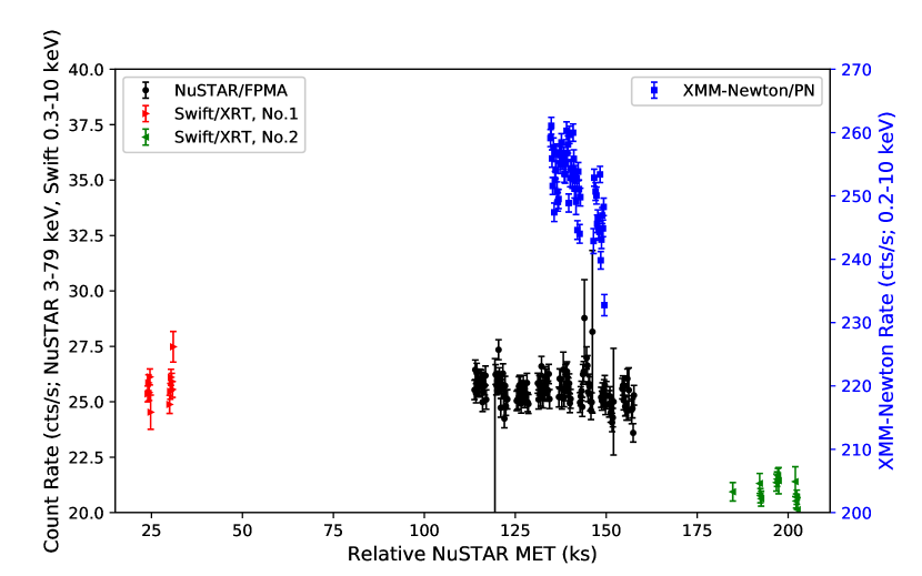
Figure 1: Light curves of Swift/XRT (0.3-10 keV), NuSTAR/FPMA (3.0-79.0 keV), and XMM-Newton/EPIC-PN (0.2-10 keV) during the first observation in 2015, bin-time: 200 s. Swift/XRT, No.1 and No.2 refer to Swift obs.ID of 00032898123 and 00032898124, which were both taken within a day from NuSTAR’s start time. The reference time is $1.7835\times 10^{8}$s (NuSTAR MET, also 2015-08-27 05:39:58 UTC or 57261 MJD).

Table 1: NuSTAR and Swift observations in the 2015 and 2013 outburst cycles, exposure times and start time. WT: windowed timing mode, PC: photon counting mode.

outburst	No.	$F_{2-10keV}$	$L/L_{edd}$	NuSTAR			Swift
		($10^{-10}$ergs/cm2s)	(%)	obs.ID	S.T.	exp.(ks)	obs.ID	S.T.	exp.(ks)	mode
2015	1	6.92	2.0	80102011002	08-28 13:06	21.6	00032898124	08-29 08:55	1.7	WT
	2	5.64	1.8	80102011004	09-02 12:36	18.3	00032898126	09-03 00:37	2.3	WT
	3	4.77	1.7	80102011006	09-07 14:51	19.8	00032898130	09-07 00:21	2.8	WT
	4	3.66	1.2	80102011008	09-12 15:46	21.5	00081534001	09-12 16:18	2.0	WT
	5	2.54	1.0	80102011010	09-17 10:06	38.5	00032898138	09-17 00:06	2.3	WT
	6	1.32	0.5	80102011012	09-30 01:11	41.3	00081534005	09-30 05:32	2.0	PC
2013	1	3.44	1.4	80001013002	08-11 23:46	42.3	00032490015	08-12 00:33	1.1	WT
	2	5.68	2.4	80001013004	08-16 17:01	47.4	00080180001	08-16 18:22	1.9	WT
	3	8.70	3.6	80001013006	08-24 12:36	43.4	00080180002	08-24 04:02	1.6	WT
	4	11.85	4.6	80001013008	09-03 09:56	61.9	00032898013	09-02 19:03	2.0	WT
	5	2.06	0.8	80001013010	10-16 23:51	98.2	00032988001	10-17 11:57	9.6	WT

Notes.
Luminosity calculated using unabsorbed flux between $0.1-300$ keV, assuming a distance of 8 kpc and a black hole mass of 10  $M_{\odot}$.

2.1 NuSTAR

The NuSTAR data were reduced using the Data Analysis Software (NUSTARDAS) 1.7.1, which is part of HEASOFT 6.21 and CALDB version 20170614. Source spectra were extracted from 100^′′ circular extraction regions centered on the source position, and background spectra from 135^′′ circular regions from the opposite corner of the detector. We binned the spectra from NuSTAR’s focal point modules A and B (FPMA and FPMB) to oversample the spectral resolution by a factor of 3, to 1 minimal count per bin for C-statistics. We fitted the spectra over the whole energy range (3–79 keV) using the C-statistics.

2.2 Swift

The Swift/XRT data were processed with standard procedures (xrtpipeline 0.13.3), filtering and screening criteria using FTOOLS 6.21. The data collected in the windowed timing mode were not affected by pile-up, so source events were accumulated within a circle with the radius of 20 pixels (1 pixel $\sim$ 2.36^′′), background events within an annular region with an outer radius of 110 pixels and inner radius of 90 pixels. For the last 2015 data collected in the photon counting mode, pile-up problem is a concern, so we fitted the PSF profile with a King function in the wings, then extrapolated to the inner region and saw the divergence resulting from pile-up. We accordingly excluded a circular region with radius of 5 pixels from the source extraction region. For the response matrix, we used the response files swxwt0to2s6_20131212v015.rmf, swxwt0to2s6_20130101v015.rmf for the observations in 2015 and 2013, respectively. We generated the ancillary response files including a correction using the exposure maps, accounting for the effective area by xrtmkarf. The XRT spectra were rebinned also to 1 minimal count per bin. The fitted energy range is 0.5–8 keV.

All the uncertaintites quoted in this paper are for a 90% confidence range, unless otherwise stated. All spectral fitting is done with xspec 12.9.1 (Arnaud, 1996). In all the fits we use wilm set of abundances (Wilms et al., 2000), and vern photoelectric cross sections (Verner et al., 1996).

3 Spectral fitting

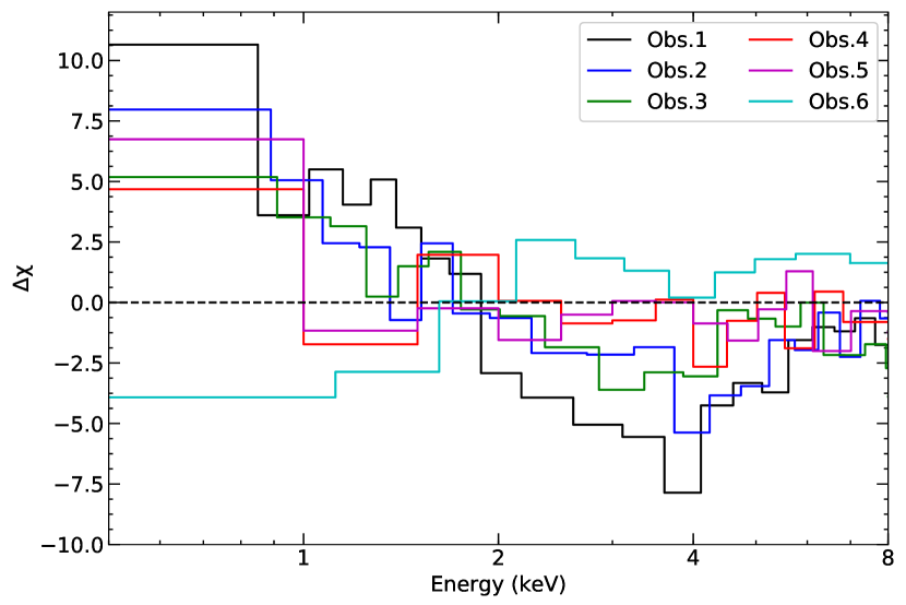
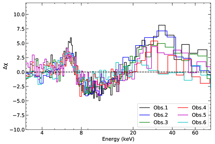
Figure 2: $\Delta\chi$ for a fit with an absorbed power-law model (i.e., tbabs*powerlaw) in the $3-8$ keV range with a fixed column density $N_{H}=5\times 10^{21}$ cm^-2 for the 2015 dataset. The disk component is present with good statistical precision in the first three observations from the Swift/XRT part (left), the iron line and Compton hump are clearly visible in all observations from the NuSTAR part (right, only FPMA data are plotted here). Data are rebinned for display clarity.

3.1 The 2015 dataset: during decay in the hard state

3.1.1 Model 1: the standard reflection model

After fitting with an absorbed power-law (i.e., tbabs*powerlaw) in the $3-8$ keV range with a fixed column density $N_{H}=5\times 10^{21}$ cm^-2, we can see from the the data-to-model ratio (Figure 2) a disk component at $\lesssim 1-2$ keV is present except for the last observation, and the iron line and Compton hump are clearly visible in all observations. Note that the total number of counts in Swift drops dramatically from $\sim 32,000$ counts (observation 3) to $\sim 4,900$ counts (observation 4), $\sim 5,300$ counts (observation 5) and $\sim 1,500$ counts (observation 6), so the statistical precision for the last three observations is relatively poor.

We perform a simultaneous fit on all six observations from 2015 using a more sophisticated model: const*Tbabs*(diskbb+nthComp+relxillCp+xillverCp) (2015-M1), where relxillCp models the relativistic reflection component and xillverCp represents the unblurred reflection coming from a distant reflection that could be wind or the outer region of a flared disk. The multi-color blackbody emission from the accretion disk is included via diskbb, and the Comptonization of the disk emission coming from the corona via nthComp. During the fit, we tie several global parameters that are expected to be unchanged during the time range for our observations ($\sim$ a month) including the column density $N_{H}$, the inclination angle $i$, and the iron abundance $A_{Fe}$. The spin parameter $a_{*}$ is fixed at its maximal allowed value of 0.998, while the inner radius is left free to vary, so that $R_{in}$ can be fully explored. The constants are introduced as cross-calibration factors, thus are frozen at 1.0 for FPMA, tied together for all FPMB spectra but allowed to vary for XRT to account for the possible differences in the flux levels since these observations are not strictly simultaneous. The reflection fractions for the blurred and unblurred reflection components are frozen at $R_{f}=-1$, their iron abundances are tied, and the ionization parameter is fixed at $log\xi=0$ in xillverCp  as the gas in the distant reflector is expected to be cold and neutral (following García et al. 2015). The seed photon temperature $kT_{bb}$ in nthcomp is tied with the temperature at inner disk radius $kT_{in}$ in diskbb. If not specified, we use a canonical emissivity profile of $\propto r^{-3}$ (i.e., emissivity index $q=3$).

The resulting ratio is shown in Figure 3 (left), the best fit parameter values in Table 2 and the model components in Figure 4 (left). As we expect from the dramatic drop in count number for the last three observations, the Swift data can not provide solid constraints on the intrinsic disk emission. However, we do obtain a decreasing trend in the disk temperature and the flux ratio between 2 and 20 keV of the disk component and the unabsorbed total one, except for the last observation which has a physically unreasonable high disk temperature $0.80^{+0.04}_{-0.10}$ keV. The truncation of the inner disk and the decrease in $R_{in}$ with increasing luminosity is a prediction of the standard paradigm for the faint hard state that a hot ADAF or other coronal flow appears when the inner edge of the disk recedes from the ISCO (Narayan & Yi, 1994; Esin et al., 1997). In our best fit, we observe that during the decay, values of $R_{in}$ are all between 3 and 15 $R_{g}$, with a tentative increase towards the end of the outburst. To test the statistical significance of this tentative variation, we perform another fit in which the inner radii except for the last one are tied together, and we find $R_{in,1-5}=1.6^{+0.4}_{-0.3}$ $R_{g}$, and $R_{in,6}=12.2^{+8.4}_{-7.7}$, with C-stat increasing by 8 and $\chi^{2}$ increasing by 21 for 4 extra d.o.f. This test suggests that the crucial value of $R_{in,6}$ determining the evolution with regard to the luminosity is not statistically significant. We also find the spectrum becomes harder with the photon index dropping from 1.72 to 1.62 when the luminosity decreases, while the ionization parameter in relxillCp is reduced from $\xi\simeq 2200$ to $\xi\simeq 900$ ergs cm s^-1.

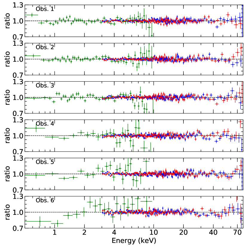
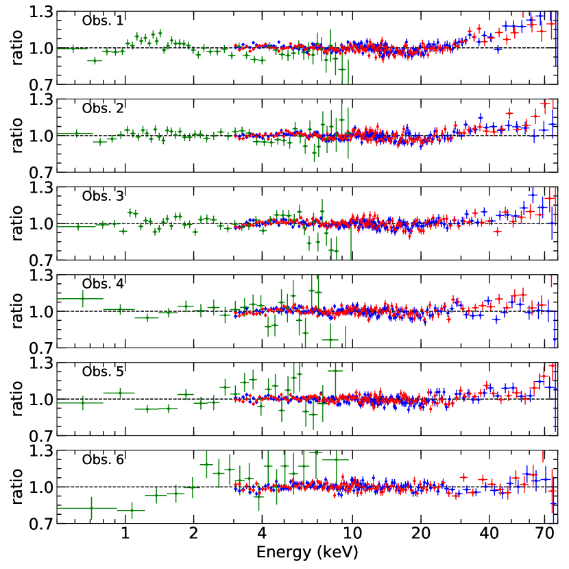
Figure 3: Data-to-model ratio for the simultaneous fit with M1 performed on the 2015 dataset with free iron abundance (left) and when the iron abundance is fixed to be the solar value (right). Discrepancy can be seen above $\sim 30$ keV when the iron abundance is fixed at the Solar value. This demonstrates the preference of these data to require large iron abundance.

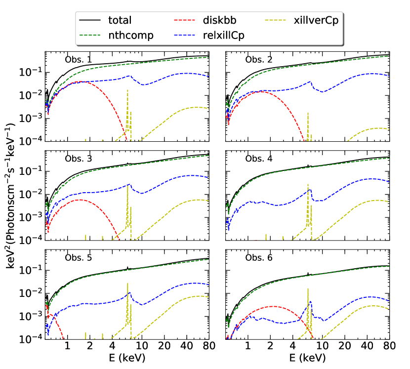
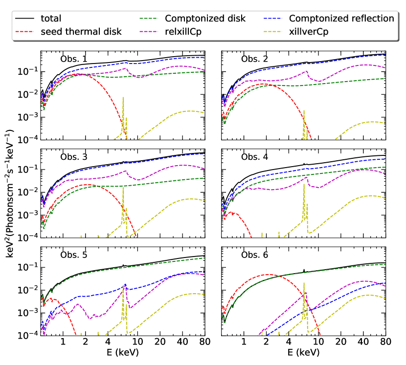
Figure 4: Model components for individual observations in 2015 for M1 (left) and M2 (right). The component each color represents is indicated in the figure. The spectrum becomes harder with the photon index dropping from 1.72 to 1.62 when the luminosity decreases. Although the statistical precision for the last three observations is relatively poor, a tentative decreasing trend in the disk temperature and the flux ratio between 2 and 20 keV of the disk component and the unabsorbed total one are shown except for the last observation.

Table 2: Best fit parameter values of model const*Tbabs*(diskbb+nthComp+relxillCp+xillverCp) in a simultaneous fit for the 2015 dataset (2015-M1).

Parameter	Obs.1	Obs.2	Obs.3	Obs.4	Obs.5	Obs.6
$N_{H}$ ($10^{21}$cm-2)	$4.12^{+0.08}_{-0.12}$
$a_{*}$	0.998
$i$ (deg)	$39.2^{+2.0}_{-1.8}$
$A_{Fe}$	$8.2\pm 1.0$
$C_{FPMA}$	$1$
$C_{FPMB}$	$1.015\pm 0.002$
$\Gamma$	$1.724^{+0.011}_{-0.009}$	$1.667^{+0.012}_{-0.009}$	$1.628^{+0.013}_{-0.014}$	$1.646^{+0.008}_{-0.019}$	$1.605^{+0.009}_{-0.010}$	$1.624^{+0.007}_{-0.013}$
$kT_{e}$ (keV)	$>195$	$>224$	$>95$	$>67$	$>152$	$46^{+35}_{-8}$
$kT_{in}(keV)$	$0.46^{+0.03}_{-0.01}$	$0.30^{+0.03}_{-0.06}$	$0.45^{+0.02}_{-0.05}$	$0.36^{+0.08}_{-0.04}$	$0.058^{+0.023}_{-0.006}$	$0.80^{+0.04}_{-0.10}$
$R_{in}$($R_{ISCO}$)	$2.5\pm 0.6$	$<2.3$	$<2.2$	$<2.4$	$3.5^{+1.4}_{-0.9}$	$12.4^{+8.4}_{-7.5}$
$log\xi$	$3.34^{+0.04}_{-0.02}$	$3.11^{+0.06}_{-0.05}$	$3.12^{+0.16}_{-0.07}$	$3.02^{+0.02}_{-0.27}$	$3.08^{+0.07}_{-0.06}$	$2.95^{+0.15}_{-0.49}$
$N_{disk}$	$170^{+41}_{-36}$	$58^{+32}_{-12}$	$30^{+12}_{-8}$	$<31$	$>3\times 10^{4}$	$<1.1$
$N_{nthComp}$	$0.103^{+0.001}_{-0.003}$	$0.107^{+0.003}_{-0.006}$	$0.072^{+0.002}_{-0.003}$	$0.066^{+0.001}_{-0.007}$	$0.049\pm 0.001$	$0.017^{+0.002}_{-0.001}$
$N_{relxillCp}$($10^{-3}$)	$1.15^{+0.16}_{-0.09}$	$1.16^{+0.24}_{-0.14}$	$0.84^{+0.18}_{-0.10}$	$0.60^{+0.25}_{-0.16}$	$0.32\pm 0.07$	$0.08^{+0.03}_{-0.02}$
$N_{xillverCp}$($10^{-5}$)	$<12$	$<10$	$7.2^{+7.6}_{-7.0}$	$7.2^{+6.2}_{-5.1}$	$9.1^{+5.0}_{-4.6}$	$3.1^{+2.1}_{-2.2}$
$C_{XRT}$	$1.017\pm 0.017$	$1.027\pm 0.012$	$1.086\pm 0.017$	$1.06\pm 0.03$	$1.044\pm 0.025$	$0.88\pm 0.04$
$L/L_{edd}$ (%)	2.0	1.8	1.7	1.2	1.0	0.5
$F_{disk}/F_{unabsorbed}$ (%)	2.0	0.8	0.4	0.005	0	1.5
$R_{s}$	0.22	0.18	0.15	0.13	$0.10$	0.04
$C-stat$	$10800$
$\chi^{2}/d.o.f.$	$12077/10730=1.126$

Notes.
Luminosity calculated using unabsorbed flux between $0.1-300$ keV, assuming a distance of 8 kpc and a black hole mass of 10  $M_{\odot}$. The flux ratio of disk emission and the total unabsorbed one is calculated in the $2-20$ keV range. The reflection strength $R_{s}$ is determined from the flux ratio between relxillCp and nthComp in the energy range of $20-40$ keV.

We also tried other emissivity profiles:

• Free emissivity index $q_{1}$ within the breaking radius $R_{br}$ free, and a fixed outer emissivity index $q_{2}=3$. We find $q_{1}$ is between the value of 3 and 4, $R_{br}$ could not be constrained and the other parameters were insignificantly affected, with the C-stat decreasing by only $\sim$23 for 12 fewer degrees of freedom.

• Free emissivity index $q_{1}=q_{2}$ all over the disk. We again find $q$ falls between 3 and 4, the other parameters were insignificantly affected, with the C-stat decreasing by only $\sim$9 for 6 fewer degrees of freedom.

• Lamppost geometry. The fit is statistically worse by a $\Delta$C-stat$=76$ for 6 fewer degrees of freedom. The corona height was found to be fairly large ($10-20R_{g}$) and poorly constrained.

We notice the large iron over-abundance in our fits: $8.2\pm 1.0$ in Solar units. To show the data prefers the over-abundance, we fix the iron abundance to be the Solar value for this dataset (2015-M1-AFe1), and find the C-stat increases by 791, for one additional degree of freedom. The disk becomes more truncated, especially for Obs.5, in which the value of $R_{in}$ increases from $4.3^{+1.7}_{-1.1}R_{g}$ to $>172R_{g}$ (see Table A1 for the best-fit parameters). To interpret this, and following the procedure in Section 6.1.4 in García et al. 2015, we plot the model components nthcomp+relxillCp for these two cases in Figure 5, which shows it could be difficult to distinguish a case with a Solar iron abundance and a disk truncated at hundreds of $R_{g}$ from the case of iron over-abundance and mild truncation, without good quality data covering the oxygen emission line below 0.7 keV and the Compton hump above 20 keV. Because of the low S/N of the Swift data, we can not probe the oxygen line. However, with NuSTAR’s wide energy coverage up to 79 keV, we can see evidence of discrepancy above $\sim 30$ keV when the iron abundance is fixed at the Solar value, as shown in Figure 3. This demonstrates the preference of these data to require large iron abundance.

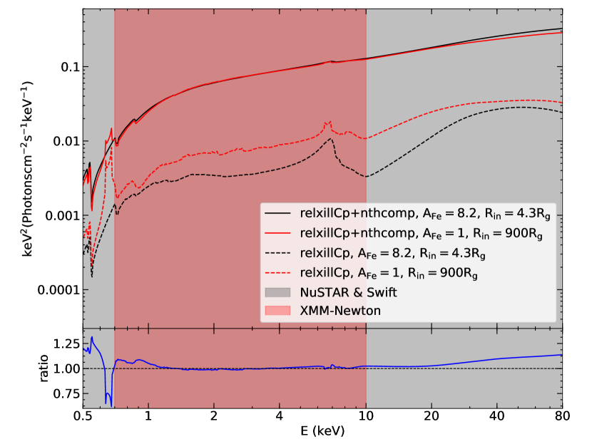
Figure 5: Model components nthcomp+relxillCp for the two cases: (1) $A_{Fe}=8.2$ and $R_{in}=4.3^{+1.7}_{-1.1}R_{g}$; (2) $A_{Fe}=1.0$ and $R_{in}=900R_{g}$. The lower panel shows the ratio between the model component nthcomp+relxillCp in case (1) and case (2). It might be difficult to distinguish these two cases when good quality data covering the oxygen emission line below 0.7 keV and the Compton hump above 20 keV are not both available.

3.1.2 Model 2: taking the Comptonization of reflection into account

The presence of a corona as the source of the hard photons in the continuum suggests the possibility for some of the reflected photons to intercept such a corona before they reach the observer. This will result in additional Compton scattering of some fraction of the reflection spectrum. As a first-order adjustment, we can convolve the reflection spectrum with a Compton-scattering kernel. For this we use the model simplcut, which adopts a scattering kernel based upon nthComp (Zdziarski et al., 1996). It has four physical parameters: the scattered fraction $f_{sc}$, the spectral index $\Gamma$, the electron temperature $kT_{e}$, and the reflection fraction $R_{f}$. We follow the procedures in Steiner et al. (2017), but we do not implement any linking between the diskbb parameters in the hard and soft states. In xspec notation, the model we adopt is:

constant*Tbabs*[simplcut*(diskbb+relxillCp)
+xillverCp] (2015-M2).

Here, in applying simplcut in this way we are assuming that the fraction of disk photons that are up-scattered in the corona is the same as the fraction of reflected photons also intercepted by the corona, as they are governed by one single scattering fraction. The best-fit parameters are shown in Table 3. For the last observation with the lowest luminosity, the fit is consistent with the whole range of inner radii, $1.5-800$ $R_{g}$, at the 90% confidence level. This might be due to that the scattering fraction is so large ($>0.97$) that the reflection features including the iron line are heavily diluted, while the unblurred reflection component xillverCp can compensate for the iron emission seen in the spectrum with a small ionization parameter ($log\xi<2.36$). The iron line profile becomes difficult to determine and thus, the inner edge of the disk is unconstrained. Also, the disk component is not evident in data.

In this framework of coronal Comptonization, there are several model components: the power-law continuum, the intrinsic disk emission, the relativistic reflection, and the Comptonized reflection. Besides the overall normalization, only two parameters determine the relative strength of each component: the scattered fraction $f_{sc}$, and the reflection fraction $R_{f}$. The former depends on the geometry of the disk-corona system and also the optical depth in the corona; while the latter is only associated with the geometry of the system. We find that $f_{sc}$ increases when the luminosity decreases (see Table 3). This could be explained by changes in the corona structure. Figure 4 (right) shows how the model components change through observations. We calculated the reflection strength as defined in Dauser et al. 2016, and find that except for observation 1, the other five observations show a decreasing trend from $\sim 4$ to $\sim 0.2$, which is in line with the increasing inner radius of the accretion disk.

Table 3: Best fit parameter values of model const*Tbabs*[simplcut*(diskbb+relxillCp)+xillverCp] in the simultaneous fit performed on the 2015 outburst dataset (2015-M2).

Parameter	Obs.1	Obs.2	Obs.3	Obs.4	Obs.5	Obs.6
$N_{H}$ ($10^{21}$cm-2)	$4.43^{+0.12}_{-0.06}$
$a_{*}$	0.998
$i$ (deg)	$39.2^{+1.6}_{-1.5}$
$A_{Fe}$	$7.7^{+1.0}_{-0.9}$
$C_{FPMA}$	1
$C_{FPMB}$	$1.0148\pm 0.0018$
$\Gamma$	$1.781^{+0.009}_{-0.008}$	$1.717\pm 0.008$	$1.663\pm 0.007$	$1.663^{+0.040}_{-0.007}$	$1.635^{+0.004}_{-0.006}$	$1.654^{+0.023}_{-0.032}$
$f_{sc}$	$0.51\pm 0.02$	$0.64\pm 0.02$	$0.68^{+0.04}_{-0.03}$	$0.66^{+0.06}_{-0.08}$	$0.45^{+0.08}_{-0.05}$	$>0.97$
$kT_{e}$ (keV)	$>196$	$>100$	$>66$	$67^{+47}_{-18}$	$>117$	$46^{+111}_{-12}$
$kT_{in}(keV)$	$0.51\pm 0.03$	$0.66^{+0.11}_{-0.12}$	$>0.57$	$<0.13$	$0.110^{+0.018}_{-0.002}$	$>0.78$
$N_{disk}$	$227^{+74}_{-26}$	$26^{+55}_{-8}$	$8^{+11}_{-2}$	$(4.8^{+1.8}_{-4.5})\times 10^{4}$	$>7.1\times 10^{4}$	$20^{+8}_{-1}$
$R_{in}$($R_{ISCO}$)	$<1.9$	$1.8^{+3.0}_{-0.6}$	$<1.9$	$<2.1$	$5.0^{+2.7}_{-1.4}$	$-$
$log\xi$	$3.29^{+0.04}_{-0.06}$	$3.07^{+0.07}_{-0.05}$	$3.17^{+0.18}_{-0.07}$	$3.04\pm 0.05$	$2.42^{+0.40}_{-0.29}$	$<2.36$
$N_{relxillCp}$($10^{-3}$)	$2.7^{+0.2}_{-0.4}$	$2.8^{+0.3}_{-0.5}$	$2.0\pm 0.4$	$1.2^{+0.2}_{-0.5}$	$0.59^{+0.15}_{-0.11}$	$<0.64$
$N_{xillverCp}$($10^{-5}$)	$<8.3$	$<7.3$	$6.5^{+4.2}_{-5.1}$	$8.0^{+4.4}_{-4.3}$	$8.5^{+4.4}_{-4.3}$	$6.8\pm 1.9$
$C_{XRT}$	$1.018^{+0.016}_{-0.015}$	$1.007\pm 0.016$	$1.091^{+0.013}_{-0.007}$	$1.038\pm 0.025$	$1.042^{+0.028}_{-0.025}$	$0.94\pm 0.04$
$L/L_{edd}$ (%)	2.0	1.8	1.7	1.2	1.0	0.5
$R_{s}$	1.87	4.16	4.13	0.83	$0.21$	0.18
$C-stat$	$10822$
$\chi^{2}/d.o.f.$	$12067/10730=1.125$

Notes.
Luminosity calculated using unabsorbed flux between $0.1-300$ keV, assuming a distance of 8 kpc and a black hole mass of 10 $M_{\odot}$. The reflection strength $R_{s}$ is determined from the flux ratio between relxillCp and nthComp in the energy range of $20-40$ keV.

3.2 The 2013 dataset: rise and decay in a failed outburst

The absorbed power-law fit on the 2013 data do not show any strong indication of the existence of a soft disk component, thus we started the fit by fixing the disk temperature to 0.05 keV. However, with free disk temperatures the fit goes down in C-stat by 725 with 10 less d.o.f., which is a significant improvement. The flux ratio in the $2-20$ keV range between the intrinsic disk emission and the unabsorbed total one is around 3%, which matches the expected faint disk in the low-hard state, but the determined disk temperatures are above 0.8 keV for the last three observations. In addition, the inner edge of the disk does not follow a one-way trend with luminosity. The best-fit parameters for this model (2013-M1) are shown in Table 4.

We then try the model taking the Comptonization of reflection into account in this dataset (2013-M2), following the same procedures as in Section 3.1.2. Compared to 2013-M1, C-stat increases by 224 with the same d.o.f. which is statistically worse; but we also notice that M2 reduced $\chi^{2}$ by 7. Additionally, this model provides a more reasonable combination of disk and power-law components. As shown in Table 5, the disk temperatures fall into a range of values closer to the expectation for this source ($kT_{in}\lesssim 0.2$ keV). In Figure 6 (right), the intrinsic disk flux becomes much smaller which is more typical for the low-hard state.

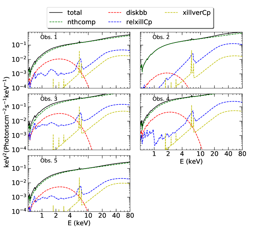
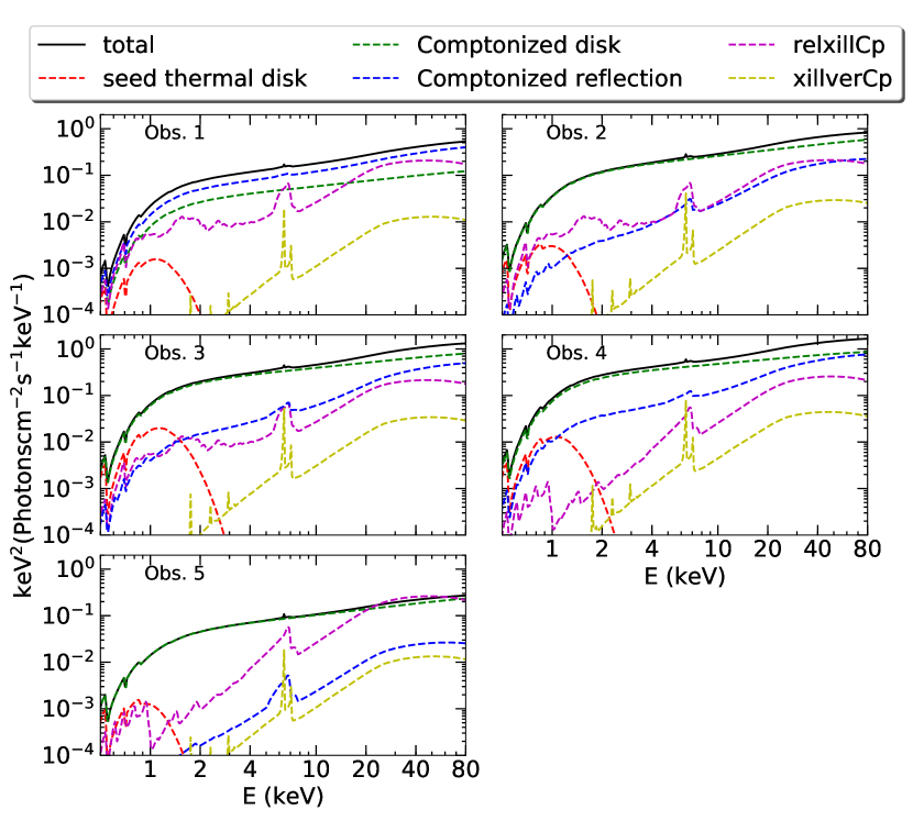
Figure 6: Model components for individual observation in 2013 for M1 (left) and M2 (right). The component each color represents is indicated in the figure. In M1, the determined disk temperatures are above 0.8 keV for the last three observations, while in M2, the disk temperatures fall into a range of values closer to the expectation for this source ($kT_{in}\lesssim 0.2$ keV), and the intrinsic disk flux becomes much smaller which is more typical for the low-hard state.

Table 4: Best fit parameter values of model const*Tbabs*(diskbb+nthComp+relxillCp+xillverCp) in a simultaneous fit performed on the 2013 outburst dataset (2013-M1).

Parameter	Obs.1	Obs.2	Obs.3	Obs.4	Obs.5
$N_{H}$ ($10^{21}$cm-2)	$4.12^{+0.06}_{-0.18}$
$a_{*}$	0.998
$i$ (deg)	$40.7^{+0.7}_{-0.8}$
$A_{Fe}$	$3.83\pm 0.06$
$C_{FPMA}$	1
$C_{FPMB}$	$1.0219\pm 0.0009$
$\Gamma$	$1.56\pm 0.02$	$1.585\pm 0.001$	$1.606\pm 0.001$	$1.54\pm 0.02$	$1.616\pm 0.001$
$kT_{e}$ (keV)	$>473$	$231^{+38}_{-21}$	$>540$	$>620$	$>497$
$kT_{in}(keV)$	$0.422\pm 0.002$	$0.53^{+0.08}_{-0.02}$	$0.892\pm 0.002$	$0.796\pm 0.001$	$0.80\pm 0.17$
$R_{in}$($R_{ISCO}$)	$<1.5$	$3.9\pm 0.8$	$14.0^{+3.5}_{-3.1}$	$10.0^{+1.6}_{-1.5}$	$32.3^{+17.2}_{-10.9}$
$log\xi$	$0.70^{+0.07}_{-0.06}$	$1.01^{+0.03}_{-0.06}$	$1.69^{+0.03}_{-0.49}$	$1.54^{+0.04}_{-0.13}$	$2.97^{+0.04}_{-0.08}$
$N_{disk}$	$3.4\pm 0.2$	$-$	$7.4\pm 0.3$	$16.8\pm 0.5$	$1.05\pm 0.05$
$N_{nthComp}$	$0.054\pm 0.019$	$0.071^{+0.014}_{-0.012}$	$0.0920\pm 0.0001$	$0.1351\pm 0.0001$	$0.02039\pm 0.00003$
$N_{relxillCp}$($10^{-3}$)	$0.63\pm 0.03$	$1.5\pm 0.2$	$2.0\pm 0.4$	$2.7\pm 0.6$	$0.23\pm 0.03$
$N_{xillverCp}$($10^{-4}$)	$2.7\pm 0.3$	$2.8\pm 0.4$	$5.0\pm 0.5$	$6.6\pm 0.4$	$1.1\pm 0.1$
$C_{XRT}$	$1.057\pm 0.025$	$1.174^{+0.015}_{-0.014}$	$0.982\pm 0.015$	$1.039\pm 0.010$	$1.074\pm 0.010$
$L/L_{edd}$ (%)	1.4	2.4	3.6	4.6	0.8
$F_{disk}/F_{unabsorbed}$ (%)	2.7	0.1	3.4	2.8	2.3
$R_{s}$	0.12	0.21	0.15	0.19	$0.09$
$C-stat$	$9556$
$\chi^{2}/d.o.f.$	$10253/9336=1.098$

Notes.
Luminosity calculated using unabsorbed flux between $0.1-300$ keV, assuming a distance of 8 kpc and a black hole mass of 10  $M_{\odot}$. The flux ratio of disk emission and the total unabsorbed one is calculated in the $2-20$ keV range. The reflection strength $R_{s}$ is determined from the flux ratio between relxillCp and nthComp in the energy range of $20-40$ keV.

Table 5: Best fit parameter values of model const*Tbabs*[simplcut*(diskbb+relxillCp)+xillverCp] in a simultaneous fit performed on the 2013 outburst dataset (2013-M2).

Parameter	Obs.1	Obs.2	Obs.3	Obs.4	Obs.5
$N_{H}$ ($10^{21}$cm-2)	$6.85^{+0.10}_{-0.09}$
$a_{*}$	0.998
$i$ (deg)	$39.7^{+2.6}_{-2.0}$
$A_{Fe}$	$2.82^{+0.17}_{-0.15}$
$C_{FPMA}$	1
$C_{FPMB}$	$1.0219\pm 0.0012$
$\Gamma$	$1.640^{+0.011}_{-0.010}$	$1.635^{+0.010}_{-0.009}$	$1.676\pm 0.006$	$1.705\pm 0.007$	$1.626^{+0.005}_{-0.004}$
$f_{sc}$	$0.78^{+0.06}_{-0.07}$	$0.69\pm 0.06$	$0.79\pm 0.03$	$0.78^{+0.02}_{-0.03}$	$0.31^{+0.05}_{-0.01}$
$kT_{e}$ (keV)	$>148$	$>159$	$>272$	$>142$	$>210$
$kT_{in}(keV)$	$0.130^{+0.011}_{-0.024}$	$0.130^{+0.006}_{-0.009}$	$0.204^{+0.008}_{-0.020}$	$0.156^{+0.006}_{-0.028}$	$0.116\pm 0.002$
$N_{disk}$($10^{4}$)	$<2.0$	$8.8^{+0.3}_{-1.0}$	$1.6^{+3.2}_{-1.3}$	$8.1^{+0.6}_{-0.7}$	$>9.4$
$R_{in}$($R_{ISCO}$)	$>11.4$	$4.4^{+1.7}_{-1.0}$	$14.3^{+7.4}_{-6.1}$	$12.6^{+4.7}_{-3.6}$	$15.6^{+14.7}_{-5.9}$
$log\xi$	$2.69\pm 0.02$	$<1.81$	$1.76^{+0.25}_{-0.34}$	$2.00^{+0.02}_{-0.12}$	$<1.78$
$N_{relxillCp}$($10^{-3}$)	$2.5^{+0.2}_{-0.9}$	$3.0^{+0.3}_{-0.6}$	$6.1^{+0.7}_{-0.6}$	$9.2^{+0.4}_{-0.5}$	$0.33^{+0.27}_{-0.09}$
$N_{xillverCp}$($10^{-4}$)	$<2.2$	$3.0^{+1.3}_{-1.6}$	$3.9^{+1.7}_{-1.8}$	$5.3^{+1.4}_{-1.5}$	$1.5\pm 0.5$
$C_{XRT}$	$1.025\pm 0.024$	$1.140\pm 0.015$	$0.947^{+0.016}_{-0.015}$	$1.012^{+0.012}_{-0.011}$	$1.028^{+0.011}_{-0.012}$
$L/L_{edd}$ (%)	1.4	2.4	3.6	4.6	0.8
$R_{s}$	1.99	0.50	0.74	0.99	$0.14$
$C-stat$	$9780$
$\chi^{2}/d.o.f.$	$10246/9336=1.097$

Notes.
Luminosity calculated using unabsorbed flux between $0.1-300$ keV, assuming a distance of 8 kpc and a black hole mass of 10  $M_{\odot}$. The reflection strength $R_{s}$ is determined from the flux ratio between relxillCp and nthComp in the energy range of $20-40$ keV.

Table 6: The intrinsic parameters of the system found in different simultaneous fits in this paper: hydrogen column density ($N_{H}$), the dimensionless spin parameter $a_{*}=0.998$ which is frozen in all through, the inclination of the inner disk $i$, the iron abundance with respect to the solar value $A_{Fe}$. The model description, C-stat and $\chi^{2}$ values are also provided.

Fit	Model Desciption	C-stat	$\chi^{2}$/d.o.f.	$N_{H}$	$i$	$A_{Fe}$
				($10^{21}$cm-2)	(deg)
2015-M1	Standard reflection model	10800	12077/10730	$4.12^{+0.08}_{-0.12}$	$39.2^{+2.0}_{-1.8}$	$8.2\pm 1.0$
	(diskbb+nthcomp+relxillCp+xillverCp)		=1.126
2015-M1-AFe1	Standard reflection model,	11591	12584/10731	$4.53^{+0.04}_{-0.05}$	$75\pm 5$	$1.0$
	$A_{Fe}=1.0$		=1.173
2015-M2	Model considering the coronal Comptonization	10822	12067/10730	$4.43^{+0.12}_{-0.06}$	$39.7^{+2.6}_{-2.0}$	$7.7^{+1.0}_{-0.9}$
	[simplcut*(diskbb+relxillCp)+xillverCp]		1.125
2013-M1	Standard reflection model	9556	10253/9336	$4.12^{+0.06}_{-0.18}$	$40.7^{+0.7}_{-0.8}$	$3.83\pm 0.06$
			=1.098
2013-M2	Model considering the coronal Comptonization	9780	10246/9336	$6.85^{+0.10}_{-0.09}$	$39.7^{+2.6}_{-2.0}$	$2.82^{+0.17}_{-0.15}$
			=1.097

4 Discussion

The parameters that are global to all observations are: the Galactic hydrogen column density $N_{H}$, the spin parameter $a_{*}$, the inclination angle $i$ and the iron abundance $A_{Fe}$. Table 6 shows a summary of these intrinsic parameter values found in different simultaneous fits performed in this paper. The inclination is consistent with $i=40\pm 2$ deg through all fits except for 2015-M1-AFe1. Assuming that the inclination of the inner disk is equal to the binary orbit inclination, with the latest measurement of the mass function $f(M)=\frac{M_{bh}\sin^{3}i}{(1+q)^{2}}=1.91\pm 0.08$ $M_{\odot}$ and $q=\frac{M_{c}}{M_{bh}}=0.18\pm 0.05$ (Heida et al., 2017), we estimate the mass of the black hole to be $M_{bh}=10.0\pm 0.6$ $M_{\odot}$.

Fürst et al. (2015) found the disk to be truncated at tens of $R_{g}$, based on the same NuSTAR and Swift dataset of the 2013 outburst, using the model constant*tbabs*[powerlaw+relconv(reflionx)+
gaussian], which includes the older reflection model reflionx (Ross & Fabian, 2005), convolved with the relativistic kernel relconv (Dauser et al., 2010). By comparing the simplcut*relxillCp with the relxillCp models shown in Figures 4 and 6 (right), the slope of the reflection component is reduced as a pure consequence of coronal scattering. This could potentially explain the results found in Fürst et al. 2015. After allowing a difference between the photon index feeding the reflection ($\sim 1.3$) and the one in the power-law continuum ($\sim 1.6$) to account for a possible physically extended corona with a non-uniform temperature profile, they found the iron abundance was also reduced (from $\sim 5$ to $\sim 1.5$), and thus, forces the disk to be much more truncated to minimize the relativistic effects that blur the line profile. Nevertheless, in our case, M2 only provides a significant reduction in the iron abundance compared to M1 for the 2013 data.

We do not observe a clear evolution for a decrease of disk temperature with decreasing luminosity, as another prediction in the truncation disk scenario. The reasons for this are threefold. First, the Swift data have the total numbers of counts much smaller than NuSTAR ($10-100$ times smaller), which makes the determination of disk temperatures governed by the low energy range very difficult. Second, the large disk temperatures we find with M1 could be artificially produced by the complexity of the Comptonization model (Kolehmainen et al., 2013). In the frequency resolved spectra, the most rapidly variable part of the flow has harder spectra and less reflection than the slowly variable emission (Axelsson et al., 2013). This feature would give rise to spectral curvature in broad-band data (as seen in, e.g., Makishima et al. 2008), and thus, requires an additional soft component when such a continuum is fitted with a single Comptonization component. Lastly, as we do not observe a strong evolution pattern of the disk’s inner radius with luminosity, it is understandable that the disk temperature does not evolve as expected either.

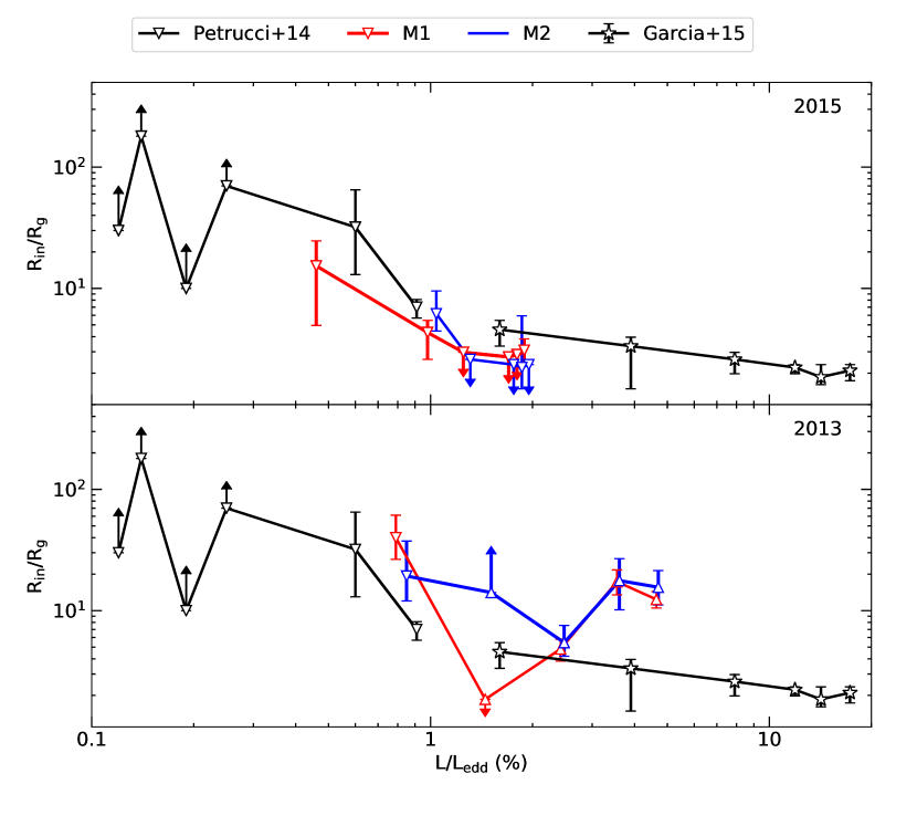
Figure 7: Comparison for GX 339–4 of our estimates (upper: the 2015 dataset, lower: the 2013 dataset) with those in the previous literature García et al. (2015) and Petrucci et al. (2014) of the inner-disk radius vs. Eddington-scaled luminosity. The luminosity values for the same observations are slightly shifted for clarity.

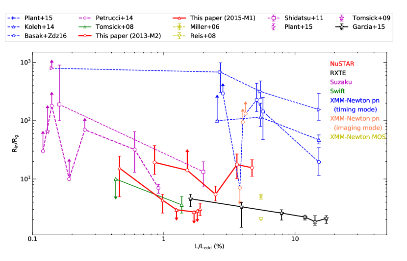
Figure 8: Comparison of the inner-disk radius vs. Eddington-scaled luminosity for GX 339–4. Our best fit values are shown in contrast with previous studies using reflection spectroscopy (Plant et al., 2015; Kolehmainen et al., 2013; Basak & Zdziarski, 2016; Petrucci et al., 2014; Tomsick et al., 2009; Miller et al., 2006; Reis et al., 2008; Shidatsu et al., 2011; Tomsick et al., 2008; García et al., 2015). Each instrument is plotted with a different color as indicated. The luminosity values for the same observations are slightly shifted for clarity.

The evolution of the inner disk radius changing with respect to the luminosity we find in different models, and those reported by García et al. (2015) and Petrucci et al. (2014) are shown in Figure 7. For a detailed summary of estimations of $R_{in}$ in previous literature for GX 339–4 between a luminosity range of $0.1\%-20\%L_{edd}$ in low-hard state obtained from the reflection spectroscopy, see Table 5 in García et al. (2015).

Among all the fits we performed, 2015-M1 shows the most promising decreasing trend of $R_{in}$ with increasing luminosity. However, this result is not statistically significant, as we suggested in Section 3.1.1. By comparing the trends M1 and M2 give for the 2015 dataset (see the upper panel in Figure 7), except for the one missing data point in M2 where $R_{in}$ is unconstrained, the other five values agree well with each other, suggesting a consistent and model-robust conclusion.

Another interesting aspect to notice is that in the luminosity range covered by the two datasets, the values of $R_{in}$ found for the 2013 observations is slightly larger. This could be due to the fact that the 2013 observations were taken in the rising phase (obs.1-4), and at the end of a failed outburst (obs.5), while the 2015 data was taken during the decay of a successful one. The hysterisis pattern typically observed in the hardness-intensity diagram of this source suggests that the evolution during the rising and decay phases displays a different phenomenology, which is likely to affect the evolution of the inner radius.

The evolution of $R_{in}$ with luminosity in the low-hard state is a matter of central importance for the study of black hole binaries. As our results are limited by the relatively small luminosity range we explore, we plot the reported results in previous literatures and our preferred ones (2015-M1 and 2013-M2) of inner radius vs. Eddington-scaled luminosity in Figure 8, sorted and colored with regard to satellites, instruments, and observation mode. At luminosities larger than 1% $L_{edd}$, there are two groups of results: an upper group with inner radii between $20R_{g}$ and $800R_{g}$ comprised by values from XMM-Newton pn timing mode and two imaging mode data; and a bottom group with $R_{in}<20R_{g}$ aligned with NuSTAR , RXTE , Suzaku , Swift , XMM-Newton MOS and one XMM-Newton pn imaging mode data. These results indicate the possibility of calibration issues with XMM-Newton pn timing mode data as the main factor responsible for the very extreme truncation.

5 Conclusions

We have analysed eleven observations of GX 339–4 in the low-hard state seen by NuSTAR and Swift , five taken in a failed outburst in 2013 and the other six during the decay of the 2015 outburst. The luminosity covers the range of 0.5% to 5% $L_{edd}$, which only covers a fraction of the usual luminosity range typically observed during the outburst for this source (up to $20-30\%$ $L_{edd}$). Each spectrum spans the energy range 3–79 keV from NuSTAR, and 0.5–8 keV from Swift. The data have in total 10.7 million counts, and a composed exposure time of 790 ks.

Both datasets are fitted with two models: a standard reflection model including intrinsic disk emission, power-law continuum, and both the relativistic and unblurred reflection components const*Tbabs*(diskbb+nthComp+relxillCp+xillverCp) (M1); and a model in which the reflection component is Comptonized by the corona constant*Tbabs*[simplcut*(diskbb+relxillCp)
+xillverCp].

During the decay in 2015, with fit M1 we find that the inner disk recedes from the ISCO, values of $R_{in}$ are all between 3 and 15 $R_{g}$, with a tentative increase towards the end of the outburst, although we do notice that the largest truncation radius here is not statistical significant. Fit M2 provides similar results, except for the last observation whose inner radius is unconstrained. As for the 2013 dataset, the disk temperatures determined from M1 are unphysically large for these luminosities in the low-hard state, while M2 can effectively reconcile these values ($kT_{in}\lesssim 0.2$ keV) and provide more physical trends. The evolution of $R_{in}$ with luminosity for the 2013 data is somewhat less monotonic than for the 2015, and while the inner radius is larger in the former, we find the largest disk truncation is constrained to be less than $37R_{g}$ when the source is at 0.8% $L_{edd}$.

Part of this work was carried out by JW during attendance to the Summer Undergraduate Research Fellowship (SURF) at California Institute of Technology in 2017. Warm hospitality and tutelage are kindly acknowledged, in particular from the members of the NuSTAR Science Operations Team (K. Foster, B. Grenfestette, K. Madsen, M. Heida, M. Brightman, and D. Stern). We would like to thank the referee for useful comments towards the improvement of this paper. We also thank B. de Marco and G. Ponti for useful discussions. JAG acknowledges support from NASA grants NNX17AJ65G and 80NSSC177K0515, and from the Alexander von Humboldt Foundation. JFS has been supported by NASA Hubble Fellowship grant HST-HF-51315.01. SC is supported by the SERB National Postdoctoral Fellowship (No. PDF/2017/000841). We thank the NuSTAR Operations, Software, and Calibration teams for support with the execution and analysis of these observations.

Table A1 shows the best-fit parameters when we fix the iron abundance to be the Solar value for the 2015 observations (2015-M1-AFe1). The disk becomes more truncated, especially for Obs.5, in which the value of $R_{in}$ increases from $4.3^{+1.7}_{-1.1}R_{g}$ to $>172R_{g}$. However, the fit is significantly worse in statistics with regard to 2015-M1, with C-stat increasing by 791 for one additional degree of freedom. In addition, with NuSTAR’s wide energy coverage up to 79 keV, we can see evidence of discrepancy above $\sim 30$ keV, as shown in Figure 3. This demonstrates the preference of these data to require large iron abundance, and a systematic discussion about the iron over-abundance found by reflection spectroscopy will be presented in a future publication.

Table A1: Best fit parameter values of model const*Tbabs*(diskbb+nthComp+relxillCp+xillverCp) with a frozen iron abundance at the solar value in the simultaneous fit for the 2015 dataset (2015-M1-AFe1).

Parameter	Obs.1	Obs.2	Obs.3	Obs.4	Obs.5	Obs.6
$N_{H}$ ($10^{21}$cm-2)	$4.53^{+0.04}_{-0.05}$
$a_{*}$	0.998
$i$ (deg)	$75.0\pm 5.0$
$A_{Fe}$	$1.0$
$C_{FPMA}$	$1$
$C_{FPMB}$	$1.015^{+0.004}_{-0.002}$
$\Gamma$	$1.767\pm 0.002$	$1.70^{+0.05}_{-0.05}$	$1.665^{+0.006}_{-0.010}$	$1.665^{+0.007}_{-0.010}$	$1.637\pm 0.001$	$1.653\pm 0.002$
$kT_{e}$ (keV)	$>388$	$>381$	$>308$	$>250$	$>241$	$182^{+42}_{-31}$
$kT_{in}(keV)$	$<0.06$	$<0.13$	$0.31^{+0.08}_{-0.11}$	$0.34^{+0.23}_{-0.01}$	$0.059^{+0.003}_{-0.006}$	$0.752\pm 0.003$
$N_{disk}$	$-$	$-$	$<86$	$<38$	$>3.2\times 10^{6}$	$<1.08$
$R_{in}$($R_{g}$)	$<1.4$	$25.2^{+4.8}_{-8.8}$	$>18.7$	$36.1^{+9.5}_{-6.3}$	$>172$	$55.5^{+68.2}_{-17.6}$
$log\xi$	$3.321\pm 0.001$	$3.22^{+0.05}_{-0.07}$	$3.20^{+0.10}_{-0.07}$	$3.002^{+0.006}_{-0.053}$	$3.027\pm 0.006$	$2.75^{+0.02}_{-0.08}$
$N_{nthComp}$($10^{-3}$)	$75.2\pm 0.3$	$108.8^{+0.2}_{-6.4}$	$77^{+5}_{-9}$	$65.7^{+0.2}_{-14.1}$	$49.1\pm 0.1$	$17.4\pm 0.1$
$N_{relxillCp}$($10^{-3}$)	$3.509^{+0.013}_{-0.009}$	$1.9^{+1.9}_{-0.9}$	$1.9^{+0.6}_{-0.2}$	$1.10\pm 0.03$	$0.88\pm 0.02$	$0.36\pm 0.02$
$N_{xillverCp}$($10^{-4}$)	$<0.54$	$12\pm 3$	$12^{+4}_{-3}$	$9.7\pm 0.6$	$4.8\pm 0.4$	$2.0\pm 0.2$
$C_{XRT}$	$1.064^{+0.008}_{-0.011}$	$1.013^{+0.015}_{-0.009}$	$1.082^{+0.014}_{-0.015}$	$1.052^{+0.025}_{-0.024}$	$1.042^{+0.024}_{-0.023}$	$0.87\pm 0.04$
$L/L_{edd}$ (%)	2.0	1.8	1.7	1.2	1.0	0.5
$C-stat$	$11591$
$\chi^{2}/d.o.f.$	$12584/10731=1.173$

Notes.
Luminosity calculated using unabsorbed flux between $0.1-300$ keV, assuming a distance of 8 kpc and a black hole mass of 10  $M_{\odot}$.

References

- Arnaud (1996) Arnaud, K. A. 1996, in Astronomical Society of the Pacific Conference Series, Vol. 101, Astronomical Data Analysis Software and Systems V, ed. G. H. Jacoby & J. Barnes, 17
- Axelsson et al. (2013) Axelsson, M., Done, C., & Hjalmarsdotter, L. 2013, Monthly Notices of the Royal Astronomical Society, 438, 657
- Basak & Zdziarski (2016) Basak, R., & Zdziarski, A. A. 2016, Monthly Notices of the Royal Astronomical Society, 458, 2199
- Dauser et al. (2014) Dauser, T., García, J., Parker, M., Fabian, A., & Wilms, J. 2014, Monthly Notices of the Royal Astronomical Society: Letters, 444, L100
- Dauser et al. (2016) Dauser, T., García, J., Walton, D., et al. 2016, Astronomy & Astrophysics, 590, A76
- Dauser et al. (2013) Dauser, T., García, J., Wilms, J., et al. 2013, Monthly Notices of the Royal Astronomical Society, 430, 1694
- Dauser et al. (2010) Dauser, T., Wilms, J., Reynolds, C., & Brenneman, L. 2010, Monthly Notices of the Royal Astronomical Society, 409, 1534
- Done & Diaz Trigo (2010) Done, C., & Diaz Trigo, M. 2010, Monthly Notices of the Royal Astronomical Society, 407, 2287
- Esin et al. (1997) Esin, A. A., McClintock, J. E., & Narayan, R. 1997, The Astrophysical Journal, 489, 865
- Ferreira et al. (2006) Ferreira, J., Petrucci, P.-O., Henri, G., Saugé, L., & Pelletier, G. 2006, Astronomy & Astrophysics, 447, 813
- Fürst et al. (2015) Fürst, F., Nowak, M., Tomsick, J., et al. 2015, The Astrophysical Journal, 808, 122
- García et al. (2013) García, J., Dauser, T., Reynolds, C., et al. 2013, The Astrophysical Journal, 768, 146
- García & Kallman (2010) García, J., & Kallman, T. R. 2010, ApJ, 718, 695
- García et al. (2014a) García, J., Dauser, T., Lohfink, A., et al. 2014a, The Astrophysical Journal, 782, 76
- García et al. (2014b) García, J. A., McClintock, J. E., Steiner, J. F., Remillard, R. A., & Grinberg, V. 2014b, The Astrophysical Journal, 794, 73
- García et al. (2015) García, J. A., Steiner, J. F., McClintock, J. E., et al. 2015, The Astrophysical Journal, 813, 84
- Gehrels et al. (2004) Gehrels, N., Chincarini, G., Giommi, P., et al. 2004, The Astrophysical Journal, 611, 1005
- Gierliński & Done (2004) Gierliński, M., & Done, C. 2004, Monthly Notices of the Royal Astronomical Society, 347, 885
- Harrison et al. (2013) Harrison, F. A., Craig, W. W., Christensen, F. E., et al. 2013, The Astrophysical Journal, 770, 103
- Heida et al. (2017) Heida, M., Jonker, P., Torres, M., & Chiavassa, A. 2017, The Astrophysical Journal, 846, 132
- Hughes & Blandford (2003) Hughes, S. A., & Blandford, R. D. 2003, The Astrophysical Journal Letters, 585, L101
- Hynes et al. (2003) Hynes, R. I., Steeghs, D., Casares, J., Charles, P., & O’Brien, K. 2003, The Astrophysical Journal Letters, 583, L95
- Jansen et al. (2001) Jansen, F., Lumb, D., Altieri, B., et al. 2001, Astronomy & Astrophysics, 365, L1
- Kolehmainen et al. (2013) Kolehmainen, M., Done, C., & Díaz Trigo, M. 2013, Monthly Notices of the Royal Astronomical Society, 437, 316
- Makishima et al. (2008) Makishima, K., Takahashi, H., Yamada, S., et al. 2008, Publications of the Astronomical Society of Japan, 60, 585
- Markert et al. (1973) Markert, T. H., Canizares, C. R., Clark, G. W., et al. 1973, ApJ, 184, L67
- Miller et al. (2006) Miller, J., Homan, J., Steeghs, D., et al. 2006, The Astrophysical Journal, 653, 525
- Miller et al. (2010) Miller, J., D’Aì, A., Bautz, M., et al. 2010, The Astrophysical Journal, 724, 1441
- Narayan & McClintock (2008) Narayan, R., & McClintock, J. E. 2008, New Astronomy Reviews, 51, 733
- Narayan & Yi (1994) Narayan, R., & Yi, I. 1994, The Astrophysical Journal, 428, L13
- Petrucci et al. (2014) Petrucci, P.-O., Cabanac, C., Corbel, S., Koerding, E., & Fender, R. 2014, Astronomy & Astrophysics, 564, A37
- Plant et al. (2015) Plant, D., Fender, R., Ponti, G., Muñoz-Darias, T., & Coriat, M. 2015, Astronomy & Astrophysics, 573, A120
- Reis et al. (2008) Reis, R., Fabian, A., Ross, R., et al. 2008, Monthly Notices of the Royal Astronomical Society, 387, 1489
- Ross & Fabian (2005) Ross, R., & Fabian, A. 2005, Monthly Notices of the Royal Astronomical Society, 358, 211
- Shidatsu et al. (2011) Shidatsu, M., Ueda, Y., Tazaki, F., et al. 2011, Publications of the Astronomical Society of Japan, 63, S785
- Steiner et al. (2017) Steiner, J. F., García, J. A., Eikmann, W., et al. 2017, The Astrophysical Journal, 836, 119
- Steiner et al. (2010) Steiner, J. F., McClintock, J. E., Remillard, R. A., et al. 2010, The Astrophysical Journal Letters, 718, L117
- Stiele & Kong (2017) Stiele, H., & Kong, A. 2017, arXiv preprint arXiv:1706.08980
- Tomsick et al. (2009) Tomsick, J. A., Yamaoka, K., Corbel, S., et al. 2009, The Astrophysical Journal Letters, 707, L87
- Tomsick et al. (2008) Tomsick, J. A., Kalemci, E., Kaaret, P., et al. 2008, The Astrophysical Journal, 680, 593
- Verner et al. (1996) Verner, D., Ferland, G., Korista, K., & Yakovlev, D. 1996, arXiv preprint astro-ph/9601009
- Wilms et al. (2000) Wilms, J., Allen, A., & McCray, R. 2000, The Astrophysical Journal, 542, 914
- Zdziarski et al. (1996) Zdziarski, A. A., Johnson, W. N., & Magdziarz, P. 1996, Monthly Notices of the Royal Astronomical Society, 283, 193